Abstract
The continuing degradation of ecosystem functioning, particularly in areas of fast-growing economies, is a common challenge facing humanity today and a focus of global research on sustainable development. A typical fast-developing economic region in Southeastern China, namely Sunan Canal Basin of Jiangsu Province (SCBJ), was selected for this study. Based on remote sensing monitoring data of land use for five periods of 2000, 2005, 2010, 2015, and 2019, the ecosystem service value (ESV) of SCBJ was measured using the equivalent factor method, and the spatial and temporal evolution of the ESV was analyzed using contribution and spatial statistical methods. Panel quantile regression was employed to explore in depth the segmental effects of the ecosystem service influencing factors and to increase the understanding of ecosystem service influencing mechanisms. Our results showed the following: (1) From 2000 to 2019, the land use structure was stable, and the comprehensive land use dynamic degree was continuously reduced. There were significant differences in the single land use dynamic degree of each land type, especially for built-up land. (2) During the study period, the total ESV increased first and then decreased, with the decreasing regions mainly distributed in the southeast of SCBJ and the urban rapid expansion areas on both sides of the canal. (3) In areas with different levels of ESV, the influencing factors had different impact effects. The mean proximity index (MPI), i.e., land use integrity, had a significant enhancement effect at the low ESV region and a significant dampening effect at the high ESV region. As the quantile points increase, the positive effects of the annual mean temperature (ATE), annual mean precipitation (APR), and net primary productivity (NPP) on ecosystem services gradually increase, which increased the gap between high and low ESV areas, creating a “natural Matthew effect”, while the negative effects of economic density (GDP) and population density (POP) on ecosystem services gradually decreased.
1. Introduction
Ecosystem services are not only the sum of ecosystem goods and functions that support human production and livelihoods [1,2]; they are also an essential expression of the ecological benefits that result from changes in the structure and layout of land use [3]. With the globalization of the economy, urbanization, and industrialization, ecosystem services are being depleted by changes in land use, increasing population, and growing economies, which directly threaten regional ecological security [4,5]. Ecological conservation is gradually becoming an important issue in the development of countries around the world. The importance of ecosystem services concerned with human and planetary symbiosis for ecological conservation is enormous [6]. Studying the spatial evolution of ecosystem services and the intrinsic influence mechanisms is vital for safeguarding ecological security [7].
Ecosystem service value (ESV), which can measure the service capacity of an ecosystem, is the core index of studying an ecosystem. Three main assessment methods are currently used, namely monetary measurements, physical measurements, and energy analysis models [8]. The monetary form of ESV is the most widely used, as it allows aggregation and comparison between different ecosystems [9,10] and is easily understood by the population and used by policymakers [11]. The equivalence factor method was first proposed by Costanza et al. [12] and subsequently applied by a large number of scholars to assess ESV in different countries and regions [13,14,15,16]. Among them, Xie et al. from China have localized and modified the method to improve the disadvantages of the method in underestimating arable land and to better match the actual situation [16,17]. The determination of the equivalence factor coefficient is key to ESV monetization, yet the process of its determination is inevitably somewhat subjective [18]. Therefore, it is necessary to determine the appropriate equivalence factor coefficient for the actual situation in the study area when applying the method [19].
The study of the spatial pattern of regional ecosystem services and the mechanisms affecting them is more helpful in grasping the root causes of ecosystem problems and guiding regional ecological construction [20]. Studies from different perspectives have shown that the main influencing factors on ecosystem services include natural factors such as biology, climate, soils, topography, etc. [21,22,23,24]; land landscape pattern factors [25,26]; and socioeconomic factors [27,28]. In analyzing the mechanisms driving spatial variations in ESV, scholars have mainly used traditional models and methods such as geographically weighted regression, geographic model detectors, correlation models, and regression analysis [22,29]. Although these methods identify the role of ESV influence factors, they accept the underlying cognitive assumption that the relationship between the independent and dependent variables is fixed [10]. The potential for differences in the effects of influencing factors across regions with different levels of ecosystem services is ignored, which makes it difficult to uncover differences in the effects of various influencing factors on the spatial and temporal variations of ESVs [30]. Although Liu et al. (2021) revealed a segmentation effect of the ecosystem service influence factors in the Guangdong-Hong Kong-Macao Greater Bay Area [10], it remains to be further explored whether similar phenomena are found in other regions.
In summary, there has been more fruitful research on ESV, from methodological assessment and spatiotemporal characterization to the in-depth expansion of influencing factors and driving mechanisms [31]. However, studies on the spatial and temporal dynamics of ESVs need to be deepened, the interrelationships between different ecological functions have not yet been clarified, and the influencing mechanisms causing the spatial differentiation of ESVs still need to be further explored [30]. Since 1978, economic growth has continued in SCBJ, and the high intensity of economic development and urban expansion has destroyed the elements, structures, and functions of the original ecological environment, posing a considerable challenge to the construction of its ecological civilization [32]. Therefore, this paper takes SNBJ as the research object, constructs a regional ESV estimation model and a driver indicator system, and explores the differences in the effects of ecosystem service influencing factors at different ecosystem service value levels based on a panel quantile model. Specifically, our study objectives are (1) quantifying and characterizing the spatial and temporal evolution of ESV in the SCBJ from 2000 to 2019 and (2) analyzing the differences in the effects of ecosystem service influencing factors at different ESV levels using a panel quantile regression model. This study opens a new perspective for an in-depth understanding of the ESV impact mechanisms, and the results can provide precise scientific guidance for the synergistic development of socioeconomic and natural ecosystems in the SCBJ watershed and promote ecological conservation and restoration in the Yangtze River Delta.
2. Materials and Methods
2.1. Study Area
Sunan Canal is an important part of the Beijing–Hangzhou Grand Canal, an essential strategic channel for inland water transport in China. SCBJ (30°54′59″~32°15′36″, 119°13′45″~121°23′5″) is located south of the Yangtze River Delta and includes the four prefecture-level cities of Zhenjiang, Changzhou, Wuxi, and Suzhou, with a total area of about 19,600 square kilometers, which is an important part of the Yangtze River Economic Belt [33]. The region has a dense network of rivers and abundant water, with a predominantly subtropical monsoon climate and good hydrothermal conditions. Excellent natural conditions and easy access to land and water transport have made the region one of the fastest-growing and most developed economic areas in China. In recent years, the high rate of urbanization and economic development has posed a considerable challenge to constructing an ecological civilization in SCBJ, and how to achieve synergistic economic and ecological development has become a top priority for the future development of the region. The geographical location and the spatiotemporal distribution of land use types within the study area in 2019 are shown in Figure 1.
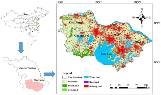
Figure 1.
Geographical location and land use of SCBJ (2019).
2.2. Influencing Factors and Data Sources
Static ecological populations and structures and dynamic ecological cycles make up entire ecosystems, and various factors directly influence them, thus changing the value of ecosystem services [7]. A review of previous research findings reveals that the factors influencing ecosystem services mainly include physical geography, land use, and socioeconomic factors [5,21]. This paper especially selects relevant influencing factors from the above three aspects.
(1) Selection of dependent variables
In this paper, the ESV of the study unit is used as the dependent variable. Land use data are employed to illustrate the ESV in the study area, which is interpreted from Land TM/ETM and Landsat 8 remote sensing imagery. Land use data for the five periods of 2000, 2005, 2010, 2015, and 2019 are obtained from the Resource and Environment Science Data Center, Chinese Academy of Sciences (http://www.resdc.cn/, accessed on 1 March 2022), at a resolution of 30 m. According to the research needs, we reclassify the land use type data into six categories: farmland, forest land, grassland, water body, built-up land, and bare land. Meanwhile, the ESVs of the study area from 2000 to 2019 are obtained by extracting, overlaying, correlating, and raster statistics in ArcGIS 10.2 in combination with grain price statistics.
(2) Selection of independent variables
In terms of natural conditions, hydrothermal conditions are an essential indicator of climatic conditions, with temperature and precipitation directly affecting the value of ecosystem services [34,35]. Net primary productivity (NPP) can indicate the state of vegetation growth and ecosystem health, which affects ecosystem cycles [36]. Therefore, the annual mean temperature (ATE), annual mean precipitation (APR), and NPP are chosen as influencing factors in this paper. Data for these variables are obtained from the National Earth System Science Data Center (http://www.geodata.cn/, accessed on 1 March 2022).
Regarding land use patterns, different land use structures generate different ecological processes and thus provide different levels of ecosystem services [37]. The mean proximity index (MPI) reflects the proximity and fragmentation of land use patches, which is inversely proportional to the fragmentation of land use structure and can characterize the structural integrity of the land [10]. Therefore, MPI is selected as the independent variable for the land use structure factor, and the data is calculated in the Patch Analyst module of ArcGIS software.
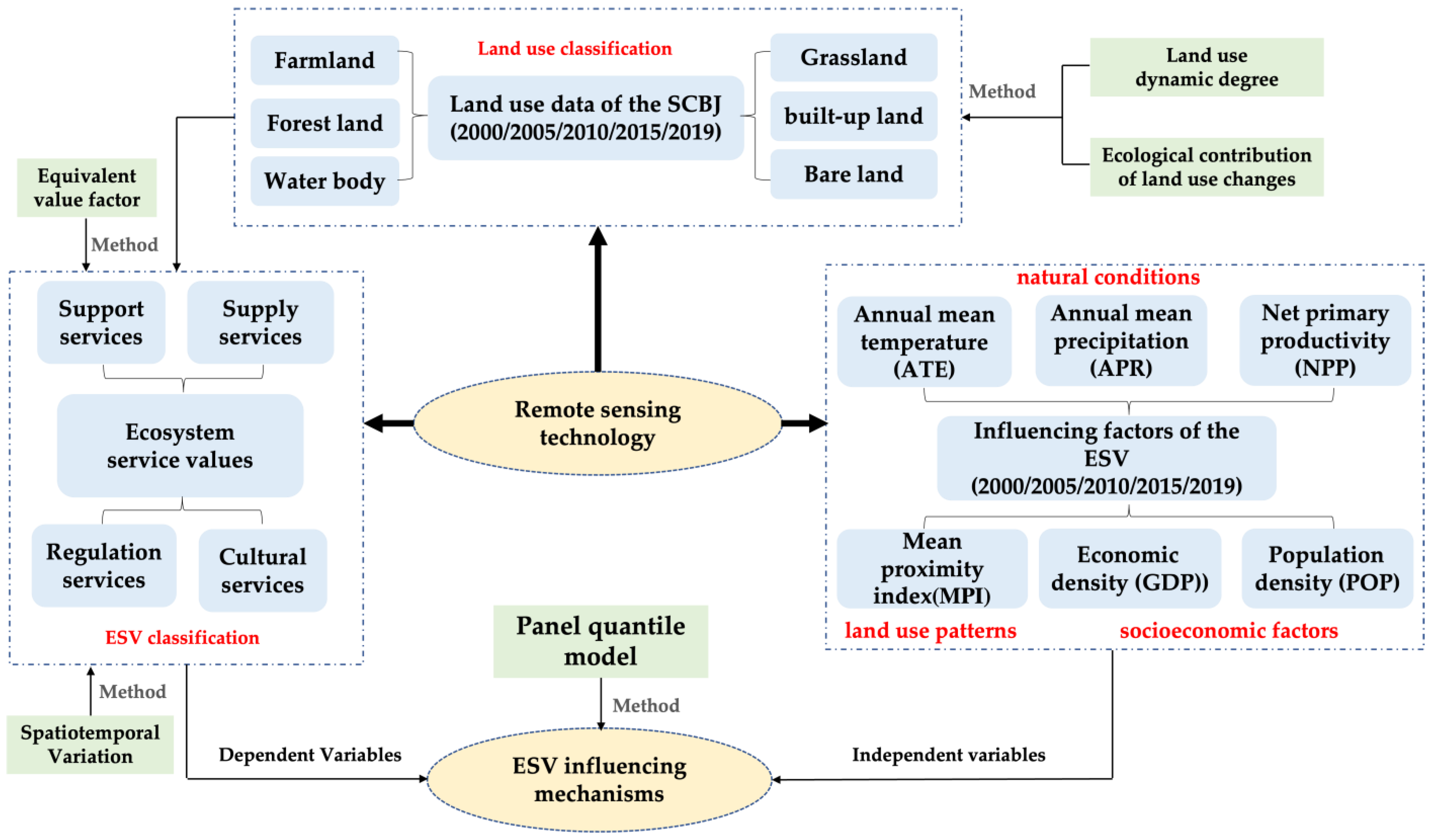
In terms of socioeconomic factors, population density (POP) indicates the intensity of daily life, and economic density (GDP) indicates the intensity of production activities. The combination of production and life can reflect the overall socioeconomic situation. Therefore, POP and GDP were selected as independent variables for the socioeconomic factors. The data for these two variables are derived from the Resource and Environmental Science Data Center, Chinese Academy of Sciences (http://www.resdc.cn/, accessed on 1 March 2022). The flow chart of this study is shown in Figure 2.
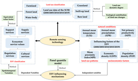
Figure 2.
Flow chart of research based on remote sensing technology.
2.3. Methods
2.3.1. Land Use Dynamic Analysis Model
To obtain the area of various land use types in each period and describe the changes in land use within the study area, this paper introduces two indicators, single land use dynamic degree (K) and comprehensive land use dynamic degree (Ks) [38], based on the analysis using ArcGIS 10.2. The formulas for calculating these two indicators are shown as follows:
where refers to the single land use dynamic degree; and represent the areas of one land use type at the start and end of the study period, respectively; and denotes the study period.
where refers to the comprehensive land use dynamic degree; denotes the absolute value of the total area converted from the jth land use type to the kth land use type in the research period, and n is the number of the land use types.
2.3.2. Estimation of ESV
The equivalence factor method, which requires relatively few data and parameters, is particularly suitable for global and regional scales, and therefore, the technique is widely used by international scholars [39]. Xie et al. proposed and improved the Chinese terrestrial ecosystem service value equivalent factor table, which had a more far-reaching impact, taking into account the regional characteristics of China [16,17]. Considering the high number of questionnaires and questionnaire return rate of the research results of Xie et al. [16], which is more credible and scientific, this paper uses it as the basic equivalent factor scale in China.
However, the nationwide factor equivalence scale was not suitable for calculating values on a regional scale. Therefore, we measured the market price of grain yields in SCBJ by referring to the statistical data from the 2020 Jiangsu Statistical Yearbook and the National Compilation of Information on Costs and Benefits of Agricultural Products. Meanwhile, the economic value of an ecological service value factor in SCBJ was calculated to be 2236.07 CNY/hm2 based on the value of ecosystem services per unit area of farmland equal to 1/7 of the average grain yield market economic value [22], and then, the base equivalent factor table applicable to the study area was obtained (Table 1). In addition, the equivalency factor for built-up land was set at zero [40]. The specific calculation formula is as follows:
where indicates the economic value of a farm ecosystem per unit of production service function (CNY/hm2). i represents food crop type and the main food crops in the study area are rice, wheat, and maize. is the national average market price of the ith food crop (CNY/t), denotes the unit yield of the -th food crop, represents the area of the ith food crop (hm2), and M is expressed as the total area of n food crops.

Table 1.
ESV equivalent factor tables for different land use types in SCBJ (CNY/hm2).
The total ESV is calculated using Equation (4):
where refers to the equivalence coefficient of the value of the jth service function per unit area of the ith land use type; represents the area of the ith land use type (hm2); i represents the number of land use types, j represents ecosystem service types, n = 6, and m = 9; and represents the ecological service value of the jth service function of the ith land use type (CNY). With the technical support of ArcGIS 10.2 software, we accounted for the ESV of the study area over 20 years using a 1km × 1km grid of evaluation cells.
2.3.3. Ecological Contribution of Land Use Changes
Changes in land use types generally reflect corresponding changes in ESV, resulting in increases or decreases in regional ESV. In this study, we used the ecological contribution model of land use type changes to quantify the response of ESV to land use type changes. In this way, we could isolate the ecological service responses associated with various land use types of change [41]. The specific calculation formula is shown below:
where is the contribution of land use type change to ESV, and are ESV equivalent factors for land use types k and j, respectively, indicates the area of land use type j converted to land use type k during the study period, and n denotes the number of all land use types in the study area.
2.3.4. Panel Quantile Model
The significant advantage of panel data is that it has both cross-sectional and temporal dimensions, which can substantially increase the panel sample size and thus significantly improve the accuracy of the model regression results [42]. Panel data regression models can identify the relationship between variables as a whole and are commonly used in the impact factor analysis, with fixed effects models and random effects models being the most widely used. However, previous panel regressions have followed the principle of Ordinary Least Squares (OLS), which is centered on mean reversion. When the data are not normally distributed or there is heteroscedasticity, the regression results are biased estimates [43]. Using quantile regression can capture the extent to which the explanatory variable ESV is affected at different quantile levels, making the estimates more robust [44].
This paper analyzed the factors influencing the change in ESV of SCBJ based on five periods of panel data from 2000, 2005, 2010, 2015, and 2019. Using the Hausman test, the fixed effects model was found to be more appropriate for this study, so we analyzed it by constructing a panel quantile model with fixed effects. Aiming at a better balance between low computational costs and high accuracy of the results, the study area was divided into a 10 km × 10 km scale grid for the regression analysis in this paper. The specific expressions are as follows [10]:
where stands for the conditional quantile function of the dependent variable ESV; indicates the quantile, ; represents the regression coefficient at quantile . , , , , , and are independent variables; represents individual effect at quantile , and its value is random but does not change with time; and denotes the random error term.
3. Results
3.1. Land Use Dynamics
By interpreting the impact of remote sensing on land use in five periods, we obtained the spatial structure distribution and area change (Figure 3 and Table 2) of land use types from 2000 to 2019. In terms of land use structure, from 2000 to 2019, the land use structure of SCBJ was dominated by farmland and water body. In 2000, the percentages of these two land types were 65.02% and 21.34%, respectively, with a total of 86.36%, while, in 2019, the percentages were 51.58% and 21.18%, respectively, with a total of 72.16%. Between 2000 and 2019, the largest change in land use was in built-up land, followed by farmland, which increased from 1785.67 km2 to 4919.67 km2 (175.5%) and decreased from 13,979.4 km2 to 11,090.6 km2 (20.7%), respectively. The area of built-up land continues to increase significantly, and in 2019, it exceeded the area of the water body for the first time. The area of water bodies first increased and then decreased, because the development and construction of cities usually built artificial lakes, allowing a slight increase in water bodies but ultimately unable to counteract the erosion of water bodies by the demands of human living space. The area of forest land also showed a continuous decrease, with the share decreasing from 5.33% in 2000 to 4.35% in 2019. The percentage of grassland and unused land was minimal, less than 0.1%.
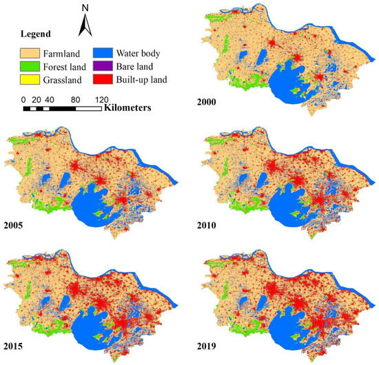
Figure 3.
Spatial distribution of land use in the study area from 2000 to 2019.

Table 2.
Area and land use change dynamics in SCBJ from 2000 to 2019.
The dynamic degree of land use change in SCBJ from 2000 to 2019 is shown in Table 2. From the single land use dynamic degree, the K value for built-up land was more significant than zero, indicating that its area was increasing, In contrast, the K values for farmland and forest land were less than zero, indicating that their area was decreasing. In particular, from 2000 to 2019, the largest dynamic value (35.85%) was recorded for built-up land, followed by unused land and grassland, with a dynamic degree of 8.78% and −3.16%, respectively. The other three land use types, farmland, forest land, and water bodies, have relatively small and negative dynamic degrees of −1.03%, −0.92%, and −0.04%, respectively. Further analysis revealed that the degree of change of construction land had a maximum value of 18.57% in stage T1 and then decreased significantly to 3.73% in stage T4, while the change of farmland also showed the same decreasing trend. The changes in grassland and water body were greater than zero in stages T1 and T2 and less than zero in stages T3 and T4. Although unused land also increased to some extent, its total area was small and, thus, did not become the primary land use type affecting regional ecosystem change.
In terms of comprehensive land use dynamic degree, the value of Ks between 2000 and 2019 is 0.73%, among which, it decreases from 0.95% at T1 to 0.37% at T4, showing an apparent decreasing trend, especially after 2015, when the value of Ks decreases significantly from 0.71% to 0.37%. This indicates a gradual slowdown in the rate of land use change in SCBJ, especially after 2015, when there was a significant slowdown in the impact of regional socioeconomic activities on land. Although farmland land has been invaded and the built-up land area has expanded rapidly, the implementation of ecological restoration projects such as “returning farmlands to forests, grasslands, and lakes” has played a significant positive role (for more details, see Zhu et al., 2022 and the website http://www.jiangsu.gov.cn/art/2013/9/5/art_46718_2590999.html, accessed on 1 April 2022).
3.2. Spatiotemporal Variation of ESV
3.2.1. Time Series Analysis of ESV
Referring to Table 3, the results indicated that the ESV of SCBJ showed a trend of first increasing and then decreasing from 2000 to 2019. Since the 21st century, the total ESV decreased from 819.18 × 10⁸ CNY in 2000 to 749.08 × 10⁸ CNY in 2019, with a decrease rate of 8.56%. The rapid urbanization of SCBJ, the significant increase in built-up land, domestic pollution, and agricultural pollution have accelerated the process of eutrophication in the water bodies of Taihu Lake, putting enormous pressure on the ecological environment. In particular, the outbreak of blue algae in Taihu Lake in 2007 caused a significant decrease in total ESVs in SCBJ [45,46].

Table 3.
Structure change of ESV from 2000 to 2019.
Our results show that the ESV of SCBJ increased by 10.71 × 10⁸ CNY from 2000 to 2005, a growth rate of 1.31%, and began to decline after 2005. The ESV decreased by 13.0 × 10⁸, 36.45 × 10⁸, and 3.137 × 10⁸ CNY in the T2, T3, and T4 periods, respectively, and the rate of decrease (−4.46%) was most remarkable in T2. In 2015, “Jiangsu Province Land Use Master Plan Management Measures” came into effect, clearly stating the need to protect and improve the ecological environment, guarantee the sustainable use of land, improve land utilization, and comprehensively promote the conservation and intensive use of land. Meanwhile, the Jiangsu Ecological River and Lake Action Plan (2017–2020) was formulated. In addition, with an emphasis on green and sustainable development, SCBJ continued to curb the deterioration of the ecological environment by accelerating the upgrading of industrial structures and ecological environment management. Generally speaking, the decrease of ESV in SCBJ has slowed down and is moving towards a harmonious coexistence between people and the environment.
3.2.2. Structure Analysis of ESV
In terms of the structure of ESVs, from 2000 to 2019, the value ratio of the four first-level subservices remained stable, and the value share of the regulation services was the highest at about 69%, which indicated that the ecosystem of SCBJ mainly plays the role of dissipating human pollution and ensuring ecosystem stability. The value of supply services was the smallest, with an annual average value of less than 60 × 108 CNY, which was closely related to the industrial characteristics of the SCBJ region, dominated by the development of manufacturing and service industries. The statistical results showed that the value of all four subservices declined from 2000 to 2019, with the decline rates of 17.35%, 6.42%, 14.61, and 4.23%, respectively, of which the supply services had the largest decline (Table 3). The estimation of single ESV changes at five-year intervals showed a gradual slowdown in decline in the value of supply and support services, while the value of regulation and cultural services presented a deteriorating trend of first growth and then decrease.
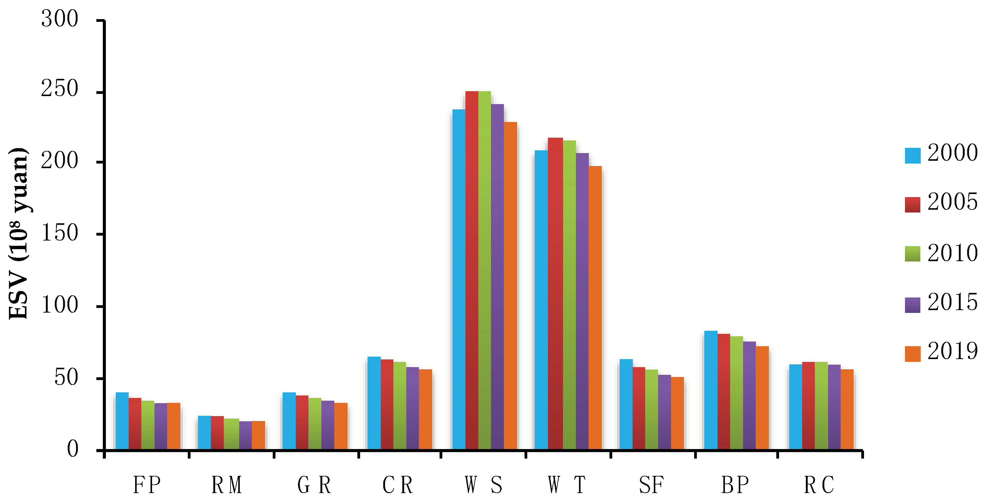
The results of secondary ecosystem service accounting showed that WS services were the dominant ecosystem service type in SCBJ from 2000 to 2019, and WT services ranked second, with an inverted “U”-shaped trend of increasing and then decreasing. The growth rates of the other seven types of ESV were all negative, among which SF services (18.86%) declined the fastest and WS services (3.59%) the slowest. The decline rates for FP, RM, GR, CR, WT, BP, and RC were 17.66%, 16.86%, 17.32%, 13.43%, 5.36%, 11.35%, and 4.23%, respectively (Figure 4).
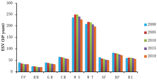
Figure 4.
Changes in ESV under the secondary classification of SCBJ from 2000 to 2019. Note: Acronyms are defined as Food production (FP), Raw material production (RM), Gas regulation (GR), Climate regulation (CR), Water supply (WS), Waste treatment (WT), Soil formation and protection (SF), Biodiversity protection (BP), and Recreation and culture (RC).
3.2.3. Spatial Distribution of ESV
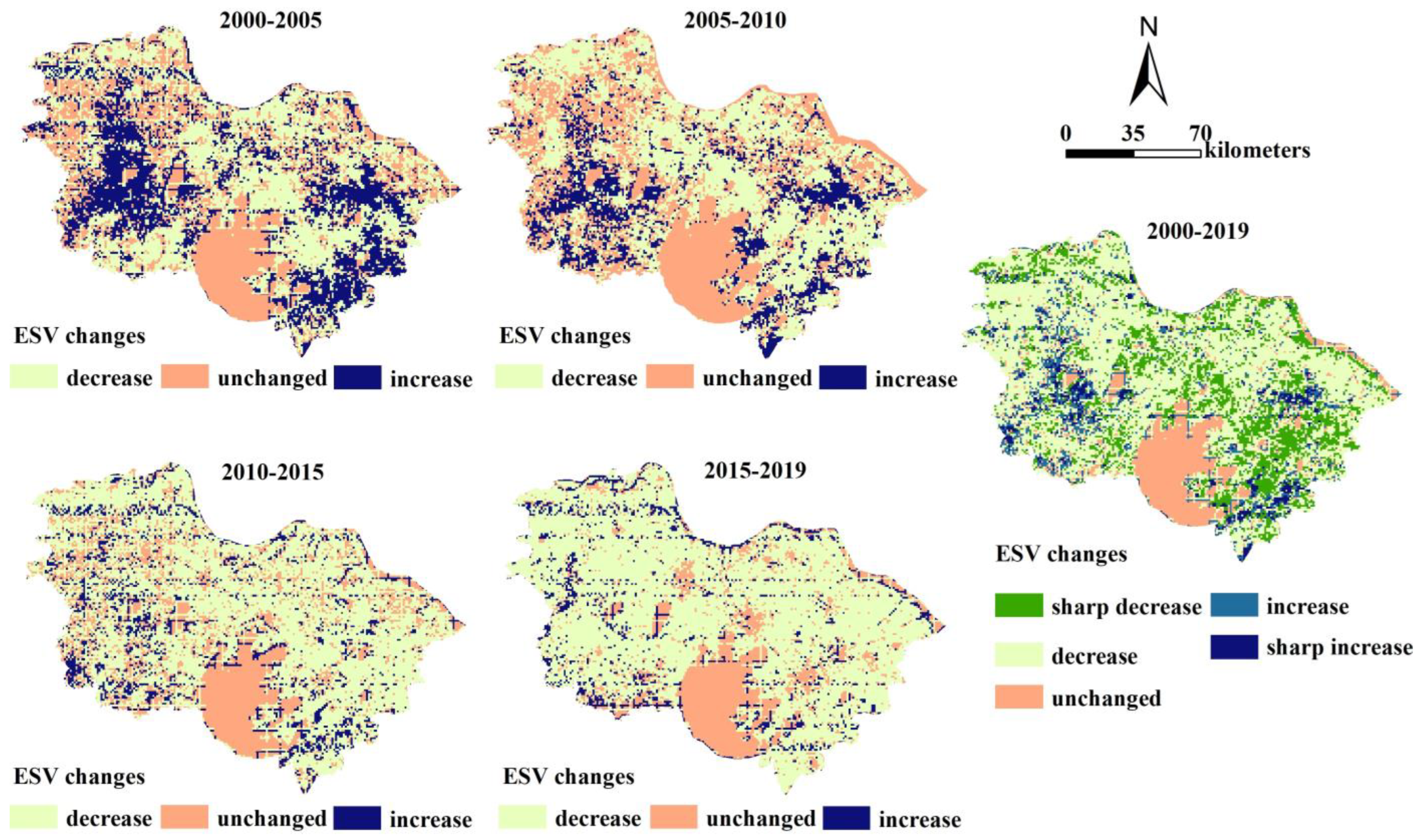
Different assessment scales impact the ESV spatial distribution, and usually, the smaller the evaluation cell is, the more accurate the ESV spatial distribution obtained is [22,47]. In this paper, the grid scale of 1 km × 1 km was chosen to analyze the ESV spatial distribution characteristics of SCBJ, because the p-value of this scale was less than 0.001, which passed the significance test. Spatial localization of the ESV changes in the study area revealed that there was significant spatial divergence in the ESV changes in different periods (Figure 5). Between 2000 and 2005, the ESV on 57.19% of the grid in the study area declined, mainly in the central and southwestern parts of SCBJ, which overlap with the urban construction land expansion space. Simultaneously, the spatial distribution of grids with rising ESV clustered in the central and western parts of Changzhou City and the southeastern part of Suzhou City. From 2005 to 2010, the percentage of space for ESV declined to 51.67%, and the decline gradually shifted to the periphery. From 2010 to 2015, a large amount of land along the Sunan Canal transformed into urban construction land, urbanization and industrialization significantly accelerated, the percentage of space with reduced ESV further expanded to 75.09%, and the ecological environment further deteriorated.

Figure 5.
Spatial distribution of ESV changes in SCBJ from 2000 to 2019.
However, from 2015 to 2019, the space share of ESV reduction further expanded to 78.47%, and the rate of decline slowed down significantly. During this period, cities entered the “stock mining” stage of construction land, paying more attention to the efficiency of built-up land use and less encroachment on ecological land. In addition, as the low-end energy-intensive and high-polluting industries in Southern Jiangsu gradually moved to Northern Jiangsu, the pressure of environmental pollution also shifted outward. Overall, from 2000 to 2019, there was a large decline in ESV in SCBJ, with significant decreases concentrated in the southeast, of which Suzhou experienced the most severe decline. The spatial distribution of the rise in ESV only clustered in Changzhou and Suzhou on a small scale.
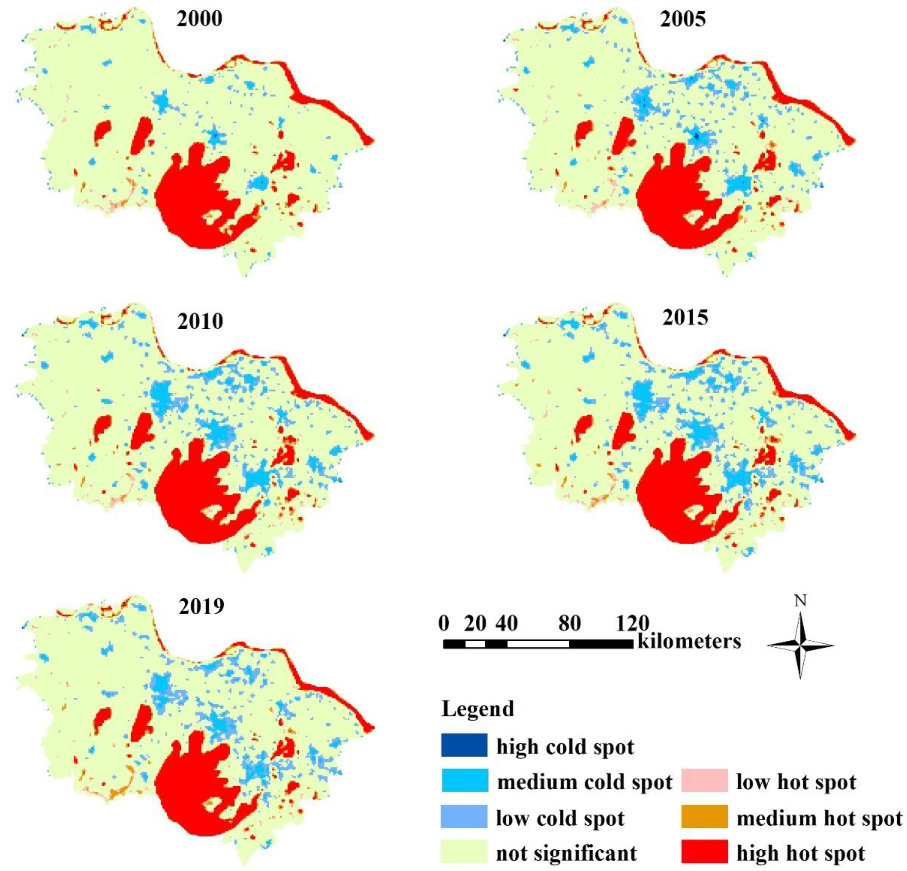
Using the hotspot analysis, we discerned the spatial clustering characteristics and evolutionary patterns of ESVs in the study area from 2000 to 2019. As can be seen from Figure 6, the spatial clustering of ESVs was not evident in most areas of SCBJ, while significant areas were dominated by the spatial clustering of high ESVs. The high hot spots of ESV were mainly concentrated in the water body area in the south, and the cold spots were primarily distributed in the central area where the built-up area was located. During the period 2000–2019, there was no significant change in the hot spot areas of ESV, while the cold spot areas gradually increased. Notably, in response to the expansion of cities, the cold spot areas increased over time, and the low-value catchment areas expanded significantly from 2000 to 2005, with the expansion areas mainly in Wuxi and Suzhou, which had the trend of “contiguous” expansion after 2010. In general, there were apparent zoning differences in ecosystem services within the SCBJ, with the central and riverine areas becoming the “front line” of urbanization and the southern water bodies becoming the “back line” of ecosystem service support.
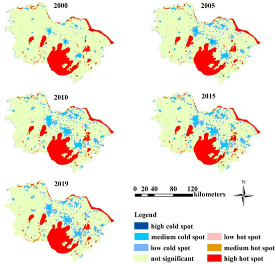
Figure 6.
Spatial clustering characteristics of ESVs in SCBJ from 2000 to 2019.
3.3. Ecological Contribution of Land Use Changes
The effect of land use type on ESV change is dynamic over a long time series. As can be seen from Table 4, the most significant ecological contribution of the different land use types in SCBJ throughout the study period came from the water body, with much higher values than the other land types. It gradually increased from 59.33% in 2000 to 65.23% in 2015 and thereafter fell to 64.46% in 2019, showing an overall trend of first increase and then decrease. The second highest ecological contribution was made by farmlands, which gradually decreased from a maximum value of 31.49% in 2000 to a minimum value of 26.53% in 2015 and then increased to 27.34% in 2019, with an overall trend of first falling and then rising. The ecological contribution of farmland began to rise after 2015 due to many farmland protection policies introduced in Jiangsu Province one after another and the incentive mechanism for farmland protection compensation becoming more and more sophisticated. The contribution of woodland continued to decline from a maximum value of 9.18% to a minimum value of 8.20%, while the ecological contribution of grassland and unused land was less than 0.01 due to their small area base. It can be seen that the water body and farmland were the most significant contributors to ESV, and the sum of their ecological contribution rates exceeded 90%. Therefore, special attention should be paid to the protection of water bodies and farmland during land development and use.

Table 4.
Different land use contribution rates (%) in SCBJ.
3.4. Segmental Effects of ESV Impact Factors
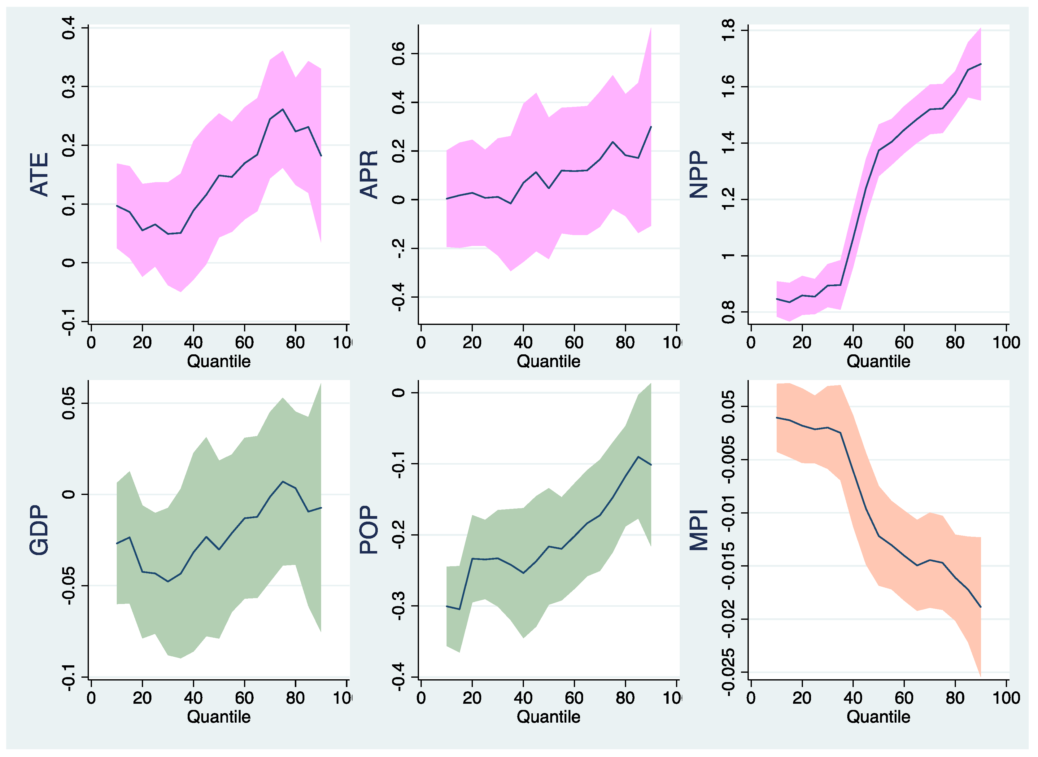
Each quantile provides a complete characterization of the distribution of ESV, and quantile regression allows visualization of the marginal effects of explanatory variables on different quartiles of ESV. Therefore, this paper employs the panel quantile regression approach to estimate the drivers of ESV in SCBJ. Five representative quartiles (i.e., 10th, 25th, 50th, 75th, and 90th) were chosen to implement the quantile regressions, and these quantile points were symmetrically distributed to facilitate the empirical analysis [48]. Meanwhile, when we divided the 10km × 10km spatial grid, many irregular cells with an area much smaller than 100 km2 emerged at the edge of SCBJ. For the sake of improving the accuracy of the results, only 177 grids with an area greater than 95 km2 were considered in this paper. To enhance the reliability of the results, we tested the smoothness of the variables, showing that the time series of the panel data is stable. Table 5 gives the results of the panel quantile regression of the ESV influences with OLS estimates in the last column, and Figure 7 presents a graph of the changes in the quantile regression coefficients of the influences.

Table 5.
Regression estimation results from a panel quantile model of ESV impact factors.
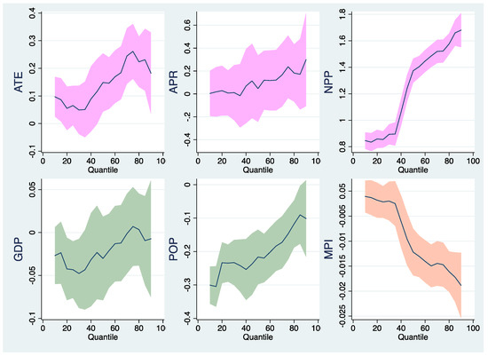
Figure 7.
Quantile regression coefficient variation diagram of influencing factors of ESV in SCBJ. Note: Acronyms are defined as Annual mean temperature (ATE), Annual mean precipitation (APR), Net primary productivity (NPP), Economic density (GDP), Population density (POP), and Mean proximity index (MPI).
According to the estimates from the panel quartile regression results (Table 5) and its quartile regression visualization (Figure 7), APR and NPP had a significant positive contribution to ESV, GDP, and POP had a significant negative inhibitory effect on ESV, while the regression coefficients for MPI and ATE appeared to change from positive to negative. In addition, the magnitude of the effect coefficients for each variable differed significantly at different quantile points.
In terms of natural conditions, the overall effect of ATE on ESV was an inverted “N” shape, with a negative (nonsignificant) effect at the 10th and 25th quartiles and a significant positive contribution effect at the other quartile points. APR and NPP had a significant boosting effect on ESV at all quantile points, with higher regression coefficients at higher quantile points than at lower quantile points, implying that the positive boosting effect increased significantly with increasing quantile. This indicated that the contribution of these variables to ecosystem service capacity enhancement was considerably more significant in the high ESV zone than in the low zone. The reason for this may be that areas of high ESV are usually more densely vegetated, which makes better use of precipitation and heat in the transfer of material and capacity, so their contribution to ESV enhancement is more significant. It is further revealed that natural conditions have a “natural Matthew effect” on ESV [10], whereby high ESV areas have a high capacity to exploit hydrothermal conditions and a high growth rate of ecosystem services, while low ESV areas have a low ability to exploit hydrothermal conditions and a low growth rate of ecosystem services. As time passes, the gap between the two becomes even wider.
Analysis of the change in MPI quantile regression coefficients showed a positive and negative shift in the effect of MPI on ESV. There was a significant positive contribution at quartiles 10th and 25th, with a significant inhibitory effect at subsequent quartile points, where the inhibitory effect gradually strengthened. It meant that in the low ESV zones, the more complete the land use structure the higher the ESV, while in the high ESV zones the opposite was true. Therefore, in low ESV regions, such as urban built-up areas, we should plan land use types rationally and intensively to conserve land to ensure structural integrity. In high ESV regions, such as undeveloped forests and water bodies, it is necessary to adopt ecological controls to avoid fragmentation of the land use structure.
For socioeconomic factors, GDP and POP have a significant negative effect on ESV, which is consistent with most academic studies [29,49]. As the quantile increases, the suppressive effect of GDP showed an inverse “N” trend of first increasing and then decreasing, while the suppressive effect of POP displayed an overall decreasing trend. It indicated that the negative impact of economic and human activities was more remarkable in high ESV areas. This finding corroborates the conclusion of the study by Liu et al. [10] We attribute this result to the fact that the high ESV areas in SCBJ tend to be undeveloped pristine waters and forests that are less affected by human and economic activities due to the treacherous terrain. Low ESV areas usually have high concentrations of humans and high economic levels, which may significantly reduce regional ecosystem services.
4. Discussion
4.1. Spatial Variation of ESV
Scientific and reasonable management of land use change has positive significance for ecosystem protection and sustainable development in SCBJ. From 2000 to 2019 the ESV in SCBJ showed a trend of first increasing and then decreasing. At the beginning of the study, the economy of southern Jiangsu had not yet fully taken off and the regional ecology was less disturbed. After 2000, the overall economic development of the region, driven by the radiation of Shanghai and surrounding cities, was rapid, and land use types with high ESV coefficients were encroached upon by land use types with low ESV coefficients. [31,32]. The area of built-up land increased by 313,400 hectares from 2000 to 2018, a dramatic increase of approximately 176%, while the area of agricultural land decreased by 288,879 hectares, a reduction of approximately 20.6%. Thanks to effective management by local governments, the regional ecological environment has shown signs of improvement and the rate of ESV decline has slowed.
The spatial distribution of ESV in SCBJ exhibited a pattern of “high in the south and low in the north”, due to the predominance of farmland in the north of the study area and the concentration of water bodies in the south. It is similar to the findings of Gao et al. (2021). In general, the unit ESV coefficients of cultivated land are much smaller than those of water bodies and are more likely to be low-value areas [9]. Regarding the ESV structure, hydrological regulation and waste treatment were the main regulating functions of SCBJ due to the large area covered by water bodies and the high ESV coefficients per unit, which had a significant positive impact on the hydrological function of the region. In SCBJ, the number of ESV cold spots grew faster in the early part of the study and slowed down in the later part, indicating that the damage caused by human activities and ecological and economic development in the area is gradually being curbed. Due to the lag in environmental recovery, the change in the number of hot spots was not significant, but the increase in the number of cold spots became significantly smaller. The interannual variation in the number of cold and hot spots was spatially consistent with the regional ESV dynamics, confirming that the deterioration of the regional ecological environment has been improved. Zhu et al. (2022) pointed out that the wetland ESV increased significantly after the implementation of the “return of fields to lakes” project, indicating that the project has an important role in improving the ecological benefits of the wetlands in the watershed and has improved the regional ecological environment to some extent [50].
4.2. Driving Factor Analysis
Explore the relationships between ecosystem services and their drivers can serve as a basis for ecosystem services management and decision-making [22] and provide an essential foundation for ecological conservation and restoration, urban and rural development, and sustainable land use [23,51]. This paper employed the panel quantile regression model to explore the drivers of ESV in SCBJ, aiming to find a more comprehensive scientific explanation of the spatial and temporal variation of ESV and enrich the research methodology of the ESV influence mechanism. The method proved to emphasize the dynamic heterogeneous trends of drivers under different ecosystem service capacities, thus avoiding the idealized model of mean reversion. It also better reflects the reality of the influence of independent variables on ESV, providing a methodological reference for a more comprehensive, systematic, and dynamic exploration of ESV driving mechanisms in the future.
As a typical wetland area with a high degree of economic development in China, the ecological environment of SCBJ, especially the watershed ecology, has continued to be unreasonably exploited by humans, resulting in the loss of ecological functions in some sections of the river. Fang et al. (2022) found that natural factors promote the formation and spatial distribution of ESVs, while anthropogenic factors such as GDP, built-up area have a negative effect [34]. Guo et al. (2022) concluded that climatic factors and land use intensity are the main factors affecting total ESV, followed by economic density and topographic conditions, and their effects have a threshold effect [20]. He et al. (2021) argued that anthropogenic disturbances have negative spillover effects on ecosystems and should be given priority consideration in regional ecological planning [52]. Yet, we were more concerned with the segmentation effect of the driving mechanism of ESV. The results of this paper revealed that, overall, the socioeconomic factors were the dominant driver of ESV change in the low ESV zone and the influence of natural conditions was relatively weak, while in the high ESV zone natural conditions became the main influencing factor of ESV change and the power of socioeconomic factors were rather weak. Low ESV zones were less able to exploit natural endowments and were more subject to human intervention, whereas the opposite was true for high ESV zones. Therefore, future ecological protection should optimize the economic development model, “develop in protection and protect in development” of high-quality ecological resources [53], as well as establish a land use pattern that combines the city and nature [54,55], to achieve the sustainable development of the regional economy.
4.3. Limitations and Future Work
This paper ignores the value of ecosystem services provided by built-up land and sets it at zero when assessing the ESV of SCBJ [16,19]. The contribution of green belts in built-up land to regional ecological services is so vital that their ecological service value cannot simply be ignored and will need to be analyzed in greater depth in future studies [15]. In addition, although ecosystems provide different types of services such as provisioning, regulation, support, and culture, this paper only explores the spatial and temporal evolution of ESV and the mechanisms driving it in SCBJ from the perspective of ESV as a whole. Research into the drivers of change in the value of different types of ecosystem services and the trade-offs and synergies with overall ESV will help to reveal the underlying causes of regional spatial and temporal variation in ESV. Therefore, the analysis of the changes in the trade-off synergistic relationship between each type of ESV and the ESV as a whole and the driving mechanisms will be the focus of the following study. The characteristics of the different drivers and the interaction and synergistic enhancement of each driver should also be considered.
4.4. Policy Implications and Suggestions
Our study shows that the ecosystem structure of the SCBJ has changed dramatically over the last 20 years, resulting in a general decrease in the various types of ESV it provides, due to a combination of natural conditions, socioeconomic factors and land use changes. They will influence the level of ecosystem functioning and provisioning capacity in the future, which plays a leading role in maintaining and enhancing human well-being [56]. Aiming to further strengthen the ecological protection of the SCBJ and promote the area’s coordinated social, economic and ecological development, we propose the following policy implications based on the study results.
Rapid social and economic development has increased the demand for construction land, which has a negative impact on the value of ecological services [7,57]. On the one hand, we should implement a farmland protection policy, strictly control the occupation of arable land for construction, and utilize construction land intensively and economically [58]. Given that the degree of land integrity in dense human areas positively contributes to ESV, ecological land fragmentation caused by high-density and fine-grained development and construction should be avoided during urban expansion. On the other hand, wetland protection, restoration and reconstruction, and reasonable utilization are incorporated into urban land use planning, making them an important part of urban infrastructure construction and realizing real ecological city construction. In addition, priority should be given to protecting the ecological environment in low ESV areas and ecologically sensitive areas, establishing wetland parks and wetland protection zones according to local conditions [59], and relying on remote sensing technology and liability systems to break the “Matthew effect” of ecosystem services.
5. Conclusions
Based on a variety of remote sensing data and grid data from 2000 to 2019, combined with statistical analysis, spatial analysis, and panel quantile regression model, the spatial-temporal evolution and driving mechanism of ESV in SCBJ were quantitatively analyzed. The most significant innovation of this study was to introduce a panel quantile model in exploring the ESV influence mechanism, which accurately identified the segmental effects of the influencing factors. Meanwhile, breaking the restriction of administrative divisions, the study area was divided into a 10km × 10km grid, which improved the accuracy of regression analysis. The main findings are as follows.
The land use structure of SCBJ remained stable, with farmland dominating, followed by water body, built-up land, forest land, and grassland, and the least amount of unused land. The land change was mainly manifested in the conversion of ecological land into land for construction, such as the transformation of farmland and forest land into building land. There were significant differences in the single land use dynamic degree by land type, particularly for built-up land, of which farmland was the primary source. The comprehensive land use dynamic degree continued to decrease over time.
The total ESV in SCBJ continued to decline between 2000 and 2019, decreasing by 7.010 billion CNY. The four categories of primary ecosystem service values had similar trends to the total values, with the highest proportion of regulating service values and hydrological regulating services, which were subordinate to regulating services, being the dominant service type in SCBJ. The two land use types, water bodies and farmland, contributed upwards to 90% of ESV and played an important role in ecosystem services.
The results of the panel quantile model indicated that the spatial variation in ESV in SCBJ was driven by a combination of natural factors, socioeconomic factors, and land use structure, with significant differences in the effects of different drivers on ESV. The positive contribution of ATE, APR, and NPP to ESV was more significant in high ESV areas than in low ESV areas, which led to a greater gap between high and low ESV areas, creating a “natural Matthew effect”. In contrast, the inhibitory effects of GDP and POP on ESV are greater in the low ESV than in the high ESV areas. MPI had a significant enhancing effect in the low ESV zone and a significant inhibiting effect in the high ESV zone. In general, socioeconomic factors were more significant in low ESV zones, while natural factors were more significant in high ESV zones.
Author Contributions
Conceptualization, X.Z. and J.S.; methodology, X.Z. and F.S.; software, X.Z.; validation, J.S. and F.S.; formal analysis, F.S. and S.W.; writing—original draft preparation, X.Z. and J.S.; writing—review and editing, X.Z., J.S. and F.S.; and supervision, J.S. and S.W. All authors have read and agreed to the published version of the manuscript.
Funding
This research was funded by the National Social Science Foundation Key Projects of China, grant number 20AJL010.
Institutional Review Board Statement
Not applicable.
Informed Consent Statement
Not applicable.
Data Availability Statement
The data that support the findings of this study are available from the corresponding author upon reasonable request.
Conflicts of Interest
The authors declare no conflict of interest.
References
- Costanza, R. Ecosystem services in theory and practice. In Routledge Handbook of Ecosystem Services; Routledge: London, UK, 2016. [Google Scholar]
- Gashaw, T.; Tulu, T.; Argaw, M.; Worqlul, A.W.; Tolessa, T.; Kindu, M. Estimating the impacts of land use/land cover changes on Ecosystem Service Values: The case of the Andassa watershed in the Upper Blue Nile basin of Ethiopia. Ecosyst. Serv. 2018, 31, 219–228. [Google Scholar] [CrossRef]
- Solomon, N.; Segnon, A.C.; Birhane, E. Ecosystem Service Values Changes in Response to Land-Use/Land-Cover Dynamics in Dry Afromontane Forest in Northern Ethiopia. Int. J. Environ. Res. Public Health 2019, 16, 4653. [Google Scholar] [CrossRef] [PubMed]
- Ridding, L.E.; Redhead, J.W.; Oliver, T.H.; Schmucki, R.; McGinlay, J.; Graves, A.R.; Morris, J.; Bradbury, R.B.; King, H.; Bullock, J.M. The importance of landscape characteristics for the delivery of cultural ecosystem services. J. Environ. Manag. 2018, 206, 1145–1154. [Google Scholar] [CrossRef] [PubMed]
- Wang, X.; Yan, F.; Su, F. Impacts of Urbanization on the Ecosystem Services in the Guangdong-Hong Kong-Macao Greater Bay Area, China. Remote Sens. 2020, 12, 3269. [Google Scholar] [CrossRef]
- Piccolo, J.J.; Taylor, B.; Washington, H.; Kopnina, H.; Gray, J.; Alberro, H.; Orlikowska, E. “Nature’s contributions to people” and peoples’ moral obligations to nature. Biol. Conserv. 2022, 270, 109572. [Google Scholar] [CrossRef]
- Liu, Z.; Wu, R.; Chen, Y.; Fang, C.; Wang, S. Factors of ecosystem service values in a fast-developing region in China: Insights from the joint impacts of human activities and natural conditions. J. Clean. Prod. 2021, 297, 12588. [Google Scholar] [CrossRef]
- STalukdar, S.; Singha, P.; Mahato, S.; Praveen, B.; Rahman, A. Dynamics of ecosystem services (ESs) in response to land use land cover (LU/LC) changes in the lower Gangetic plain of India. Ecol. Indic. 2020, 112, 106121. [Google Scholar] [CrossRef]
- He, J.; Yu, Y.; Sun, L.; Zhang, H.; Malik, I.; Wistuba, M.; Yu, R. Spatiotemporal change in the land use and ecosystem service value in the Aral Sea basin (1993–2018). Environ. Sci. Pollut. Res. 2022, 29, 74416–74427. [Google Scholar] [CrossRef]
- Liu, Z.; Wang, S.; Fang, C. Spatiotemporal evolution and influencing mechanism of ecosystem service value in the Guangdong-Hong Kong-Macao Greater Bay Area. Acta Geogr. Sin. 2021, 76, 2798–2810. [Google Scholar]
- Hoque, M.Z.; Islam, I.; Ahmed, M.; Hasan, S.S.; Prodhan, F.A. Spatio-temporal changes of land use land cover and ecosystem service values in coastal Bangladesh. Egypt. J. Remote Sens. Space Sci. 2022, 25, 173–180. [Google Scholar] [CrossRef]
- Costanza, R.; d’Arge, R.; de Groot, R.; Farber, S.; Grasso, M.; Hannon, B.; Limburg, K.; Naeem, S.; O’Neill, R.V.; Paruelo, J.; et al. The value of the world’s ecosystem services and natural capital. Nature 1997, 387, 253–260. [Google Scholar] [CrossRef]
- Troy, A.; Wilson, M.A. Mapping ecosystem services: Practical challenges and opportunities in linking GIS and value transfer. Ecol. Econ. 2006, 60, 435–449. [Google Scholar] [CrossRef]
- Dahal, R.P.; Grala, R.K.; Gordon, J.S.; Munn, I.A.; Petrolia, D.R. Geospatial Heterogeneity in Monetary Value of Proximity to Waterfront Ecosystem Services in the Gulf of Mexico. Water 2021, 13, 2401. [Google Scholar] [CrossRef]
- Meng, L.; Dong, J. LUCC and Ecosystem Service Value Assessment for Wetlands: A Case Study in Nansi Lake, China. Water 2019, 11, 1597. [Google Scholar] [CrossRef]
- Xie, G.; Zhen, L.; Lu, C. Expert knowledge based valuation method of ecosystem services in China. J. Nat. Resour. 2008, 23, 911–919. [Google Scholar]
- Xie, G.; Lu, C.; Leng, Y. Ecological assets valuation of the Tibetan Plateau. J. Nat. Resour. 2003, 18, 189–196. [Google Scholar]
- Schild, J.E.; Vermaat, J.E.; van Bodegom, P.M. Differential effects of valuation method and ecosystem type on the monetary valuation of dryland ecosystem services: A quantitative analysis. J. Arid. Environ. 2018, 159, 11–21. [Google Scholar] [CrossRef]
- Hasan, S.; Shi, W.; Zhu, X. Impact of land use land cover changes on ecosystem service value—A case study of Guangdong, Hong Kong, and Macao in South China. PLoS One 2020, 15, e0231259. [Google Scholar] [CrossRef] [PubMed]
- Guo, S.; Wu, C.; Wang, Y.; Qiu, G.; Zhu, D.; Niu, Q.; Qin, L. Threshold effect of ecosystem services in response to climate change, human activity and landscape pattern in the upper and middle Yellow River of China. Ecol. Indic. 2022, 136, 108603. [Google Scholar] [CrossRef]
- Fang, L.; Wang, L.; Chen, W.; Sun, J.; Cao, Q.; Wang, S.; Wang, L. Identifying the impacts of natural and human factors on ecosystem service in the Yangtze and Yellow River Basins. J. Clean. Prod. 2021, 314, 127995. [Google Scholar] [CrossRef]
- Pan, N.; Guan, Q.; Wang, Q.; Sun, Y.; Li, H.; Ma, Y. Spatial Differentiation and Driving Mechanisms in Ecosystem Service Value of Arid Region: A case study in the middle and lower reaches of Shule River Basin, NW China. J. Clean. Prod. 2021, 319, 128718. [Google Scholar] [CrossRef]
- Wang, H.; Zhou, S.; Li, X.; Liu, H.; Chi, D.; Xu, K. The influence of climate change and human activities on ecosystem service value. Ecol. Eng. 2016, 87, 224–239. [Google Scholar] [CrossRef]
- Wang, X.; Yan, F.; Zeng, Y.; Chen, M.; Su, F.; Cui, Y. Changes in Ecosystems and Ecosystem Services in the Guangdong-Hong Kong-Macao Greater Bay Area since the Reform and Opening Up in China. Remote Sens. 2021, 13, 1611. [Google Scholar] [CrossRef]
- Chen, W.; Zeng, J.; Zhong, M.; Pan, S. Coupling Analysis of Ecosystem Services Value and Economic Development in the Yangtze River Economic Belt: A Case Study in Hunan Province, China. Remote Sens. 2021, 13, 1552. [Google Scholar] [CrossRef]
- Msofe, N.K.; Sheng, L.; Li, Z.; Lyimo, J. Impact of Land Use/Cover Change on Ecosystem Service Values in the Kilombero Valley Floodplain, Southeastern Tanzania. Forests 2020, 11, 109. [Google Scholar] [CrossRef]
- Maimaiti, B.; Chen, S.; Kasimu, A.; Mamat, A.; Aierken, N.; Chen, Q. Coupling and Coordination Relationships between Urban Expansion and Ecosystem Service Value in Kashgar City. Remote Sens. 2022, 14, 2557. [Google Scholar] [CrossRef]
- Wilkerson, M.L.; Mitchell, M.G.; Shanahan, D.; Wilson, K.; Ives, C.D.; Lovelock, C.; Rhodes, J. The role of socio-economic factors in planning and managing urban ecosystem services. Ecosyst. Serv. 2018, 31, 102–110. [Google Scholar] [CrossRef]
- Liu, W.; Zhan, J.; Zhao, F.; Wang, C.; Zhang, F.; Teng, Y.; Chu, X.; Kumi, M.A. Spatio-temporal variations of ecosystem services and their drivers in the Pearl River Delta, China. J. Clean. Prod. 2022, 337, 130466. [Google Scholar] [CrossRef]
- Mu, X.; Guo, X.; Ming, Q.; Hu, C. Dynamic evolution characteristics and driving factors of tourism ecological security in the Yellow River Basin. Acta Ecol. Sin. 2022, 77, 714–735. [Google Scholar]
- Fang, L.; Cai, J.; Liu, Y.; Yuan, H.; Li, C. Dynamic Evolution of Ecosystem Service Value in Yangtze River Delta and Analysis on the Driving Factors. J. Ecol. Rural. Environ. 2022, 38, 556–565. [Google Scholar] [CrossRef]
- Gao, X.; Shen, J.; He, W.; Zhao, X.; Li, Z.; Hu, W.; Wang, J.; Ren, Y.; Zhang, X. Spatial-temporal analysis of ecosystem services value and research on ecological compensation in Taihu Lake Basin of Jiangsu Province in China from 2005 to 2018. J. Clean. Prod. 2021, 317, 128241. [Google Scholar] [CrossRef]
- Zhang, X.; Shen, J.; Sun, F.; Wang, S.; Zhang, S.; Chen, J. Allocation of Flood Drainage Rights in Watershed Using a Hybrid FBWM-Grey-TOPSIS Method: A Case Study of the Jiangsu Section of the Sunan Canal, China. Int. J. Environ. Res. Public Health 2022, 19, 8180. [Google Scholar] [CrossRef] [PubMed]
- He, C.; Shao, H.; Xian, W. Spatiotemporal Variation and Driving Forces Analysis of Eco-System Service Values: A Case Study of Sichuan Province, China. Int. J. Environ. Res. Public Health 2022, 19, 8595. [Google Scholar] [CrossRef] [PubMed]
- Underwood, E.C.; Hollander, A.D.; Safford, H.D.; Kim, J.B.; Srivastava, L.; Drapek, R.J. The impacts of climate change on ecosystem services in southern California. Ecosyst. Serv. 2019, 39, 101008. [Google Scholar] [CrossRef]
- Bazame, H.C.; Althoff, D.; Filgueiras, R.; Calijuri, M.L.; Oliveira, J.d.C. Modeling the Net Primary Productivity: A Study Case in the Brazilian Territory. J. Indian Soc. Remote Sens. 2019, 47, 1727–1735. [Google Scholar] [CrossRef]
- Woldeyohannes, A.; Cotter, M.; Biru, W.; Kelboro, G. Assessing Changes in Ecosystem Service Values over 1985–2050 in Response to Land Use and Land Cover Dynamics in Abaya-Chamo Basin, Southern Ethiopia. Land 2020, 9, 37. [Google Scholar] [CrossRef]
- Redo, D.J.; Aide, T.M.; Clark, M.L.; Andrade-Núñez, M.J. Impacts of internal and external policies on land change in Uruguay, 2001–2009. Environ. Conserv. 2012, 39, 122–131. [Google Scholar] [CrossRef]
- Parkes, M. Personal commentaries on “Ecosystems and human well-being: Health synthesis—A report of the Millennium Ecosystem Assessment”. Ecohealth 2006, 3, 136–140. [Google Scholar] [CrossRef]
- Yu, Q.; Feng, C.-C.; Shi, Y.; Guo, L. Spatiotemporal interaction between ecosystem services and urbanization in China: Incorporating the scarcity effects. J. Clean. Prod. 2021, 317, 128392. [Google Scholar] [CrossRef]
- Yi, L.; Zhang, Z.; Zhao, X.; Liu, B.; Wang, X.; Wen, Q.; Zuo, L.; Liu, F.; Xu, J.; Hu, S. Have Changes to Unused Land in China Improved or Exacerbated Its Environmental Quality in the Past Three Decades? Sustainability 2016, 8, 184. [Google Scholar] [CrossRef]
- Aghion, P.; Rey, H. Fixed Effects Estimation of Large-T Panel Data Models. Annu. Rev. Econ. 2018, 10, 109–138. [Google Scholar] [CrossRef]
- Akram, R.; Chen, F.; Khalid, F.; Huang, G.; Irfan, M.J.E. Heterogeneous effects of energy efficiency and renewable energy on economic growth of BRICS countries: A fixed effect panel quantile regression analysis. Energy 2021, 215, 119019. [Google Scholar] [CrossRef]
- Bandyopadhyay, A.; Rej, S.; Villanthenkodath, M.A.; Mahalik, M.K. The role of nuclear energy consumption in abatement of ecological footprint: Novel insights from quantile-on-quantile regression. J. Clean. Prod. 2022, 358, 132052. [Google Scholar] [CrossRef]
- Hu, Y.; Chen, D.; Fan, J.; Shi, Z. Evolution of landscape pattern around Taihu Lake and its influence on ecosystem services. Urban Issues 2021(04), 95–103. [CrossRef]
- Zhao, Q.; Wang, Q. Water Ecosystem Service Quality Evaluation and Value Assessment of Taihu Lake in China. Water 2021, 13, 618. [Google Scholar] [CrossRef]
- Roces-Díaz, J.V.; Vayreda, J.; Banqué-Casanovas, M.; Díaz-Varela, E.; Bonet, J.A.; Brotons, L.; de Miguel, S.; Herrando, S.; Martínez-Vilalta, J. The spatial level of analysis affects the patterns of forest ecosystem services supply and their relationships. Sci. Total Environ. 2018, 626, 1270–1283. [Google Scholar] [CrossRef]
- Liu, Y.; Lin, B.; Xu, B. Modeling the impact of energy abundance on economic growth and CO2 emissions by quantile regression: Evidence from China. Energy 2021, 227, 120416. [Google Scholar] [CrossRef]
- Song, F.; Su, F.; Mi, C.; Sun, D. Analysis of driving forces on wetland ecosystem services value change: A case in Northeast China. Sci. Total Environ. 2021, 751, 141778. [Google Scholar] [CrossRef]
- Zhu, Y.; Wang, S.; Feng, Y. Response of the Value of Wetland Ecosystem Service in Taihu Basin to the Change of Landscape Pattern in the Past 30 Years: Based on the Implementation of the Project of Restoring the Lake from the Land. Chin. Landsc. Archit. 2022, 38, 88–93. [Google Scholar] [CrossRef]
- Hu, S.; Chen, L.; Li, L.; Wang, B.; Yuan, L.; Cheng, L.; Yu, Z.; Zhang, T. Spatiotemporal Dynamics of Ecosystem Service Value Determined by Land-Use Changes in the Urbanization of Anhui Province, China. Int. J. Environ. Res. Public Health 2019, 16, 5104. [Google Scholar] [CrossRef]
- He, Y.; Kuang, Y.; Zhao, Y.; Ruan, Z. Spatial Correlation between Ecosystem Services and Human Disturbances: A Case Study of the Guangdong–Hong Kong–Macao Greater Bay Area, China. Remote Sens. 2021, 13, 1174. [Google Scholar] [CrossRef]
- Zhang, Z.; Gao, J.; Gao, Y. The influences of land use changes on the value of ecosystem services in Chaohu Lake Basin, China. Environ. Earth Sci. 2015, 74, 385–395. [Google Scholar] [CrossRef]
- Lawler, J.J.; Lewis, D.J.; Nelson, E.; Plantinga, A.J.; Polasky, S.; Withey, J.C.; Helmers, D.P.; Martinuzzi, S.; Pennington, D.; Radeloff, V.C. Projected land-use change impacts on ecosystem services in the United States. Proc. Natl. Acad. Sci. USA 2014, 111, 7492–7497. [Google Scholar] [CrossRef] [PubMed]
- Bryan, B.A.; Ye, Y.; Zhang, J.; Connor, J.D. Land-use change impacts on ecosystem services value: Incorporating the scarcity effects of supply and demand dynamics. Ecosyst. Serv. 2018, 32, 144–157. [Google Scholar] [CrossRef]
- Liu, J.; Chen, L.; Yang, Z.; Zhao, Y.; Zhang, X. Unraveling the Spatio-Temporal Relationship between Ecosystem Services and Socioeconomic Development in Dabie Mountain Area over the Last 10 years. Remote Sens. 2022, 14, 1059. [Google Scholar] [CrossRef]
- Renard, D.; Rhemtulla, J.M.; Bennett, E.M. Historical dynamics in ecosystem service bundles. Proc. Natl. Acad. Sci. USA 2015, 112, 13411–13416. [Google Scholar] [CrossRef] [PubMed]
- Wu, C.; Chen, B.; Huang, X.; Wei, Y.H.D. Effect of land-use change and optimization on the ecosystem service values of Jiangsu province, China. Ecol. Indic. 2020, 117, 106507. [Google Scholar] [CrossRef]
- Chuai, X.; Huang, X.; Wu, C.; Li, J.; Lu, Q.; Qi, X.; Zhang, M.; Zuo, T.; Lu, J. Land use and ecosystems services value changes and ecological land management in coastal Jiangsu, China. Habitat Int. 2016, 57, 164–174. [Google Scholar] [CrossRef]
Disclaimer/Publisher’s Note: The statements, opinions and data contained in all publications are solely those of the individual author(s) and contributor(s) and not of MDPI and/or the editor(s). MDPI and/or the editor(s) disclaim responsibility for any injury to people or property resulting from any ideas, methods, instructions or products referred to in the content. |
© 2022 by the authors. Licensee MDPI, Basel, Switzerland. This article is an open access article distributed under the terms and conditions of the Creative Commons Attribution (CC BY) license (https://creativecommons.org/licenses/by/4.0/).


