Article

Landsat-Scale Regional Forest Canopy Height Mapping Using ICESat-2 Along-Track Heights: Case Study of Eastern Texas

Department of Ecology and Conservation Biology, Texas A&M University, College Station, TX 77843, USA
*
Author to whom correspondence should be addressed.
Remote Sens. 2023, 15(1), 1; https://doi.org/10.3390/rs15010001
Submission received: 24 November 2022 / Revised: 10 December 2022 / Accepted: 16 December 2022 / Published: 20 December 2022

Abstract

:
Spaceborne profiling lidar missions such as the Ice, Cloud, and land Elevation Satellite-2 (ICESat-2) are collecting direct elevation measurements, supporting the retrieval of vegetation attributes such as canopy height that are crucial in forest carbon and ecological studies. However, such profiling lidar systems collect observations along predefined ground tracks which limit the spatially complete mapping of forest canopy height. We demonstrate that the fusion of ICESat-2 along-track canopy height estimates and ancillary Landsat and LANDFIRE (Landscape Fire and Resource Management Planning Tools Project) data can enable the generation of spatially complete canopy height data at a regional level in the United States. We developed gradient-boosted regression models relating canopy heights with ancillary data values and used them to predict canopy height in unobserved locations at a 30 m spatial resolution. Model performance varied (R2 = 0.44 − 0.50, MAE = 2.61–2.80 m) when individual (per month) Landsat data and LANDFIRE data were used. Improved performance was observed when combined Landsat and LANDFIRE data were used (R2 = 0.69, MAE = 2.09 m). We produced a gridded canopy height product over our study area in eastern Texas, which agreed moderately (R2 = 0.46, MAE = 4.38 m) with independent airborne lidar-derived canopy heights. Further, we conducted a comparative assessment with the Global Forest Canopy Height product, an existing 30 m spatial resolution canopy height product generated using GEDI (Global Ecosystem Dynamics Investigation) canopy height and multitemporal Landsat data. In general, our product showed better agreement with airborne lidar heights than the global dataset (R2 = 0.19 MAE = 5.83 m). Major differences in canopy height values between the two products are attributed to land cover changes, height metrics used (98th in this study vs 95th percentile), and the inherent differences in lidar sampling and their geolocation uncertainties between ICESat-2 and GEDI. On the whole, our integration of ICESat-2 data with ancillary datasets was effective for spatially complete canopy height mapping. For better modeling performance, we recommend the careful selection of ICESat-2 datasets to remove erroneous data and applying a series of Landsat data to account for phenological changes. The canopy height product provides a valuable spatially detailed and synoptic view of canopy heights over the study area, which would support various forestry and ecological assessments at an enhanced 30 Landsat spatial resolution.

Graphical Abstract

1. Introduction

Forests play a critical role in the terrestrial carbon cycle and offer a wide range of ecosystem services. The precise characterization of forest productivity, biomass, and structure is essential for understanding ecosystem responses to climatic and anthropogenic changes, but depends on our ability to accurately quantify basic forest parameters such as canopy height [1]. Improved forest canopy height estimates would lead to better forest aboveground biomass and timber volume estimates and enable improved monitoring of the effects of forest degradation and assessment of the success of forest restoration [2,3]. National forest inventory programs routinely collect canopy height measurements through field campaigns and, to a limited extent, using airborne lidar data to meet national forest inventory missions [4]. Airborne lidar data have demonstrated their effectiveness in estimating forest canopy heights but are limited for regional scale mapping due to the prohibitive cost and lower data collection efficiency. However, the increasing need to characterize forest parameters to reduce uncertainties in forest carbon estimates over large areas motivates the production of improved regional products [1]
Current spaceborne lidar acquisitions from missions such as Ice, Cloud, and land Elevation Satellite-2 (ICESat-2), with an improved sampling capability, are enhancing our capacity to characterize the three-dimensional (3D) structure of terrestrial landscapes from local to global scales [5]. ICESat-2, a photon-counting lidar mission developed by NASA (National Aeronautics and Space Administration), launched on September 2018 and is supporting the development of various elevation data products over glacial and land surfaces [6]. The ICESat-2 lidar sensor, the Advanced Topographic Laser Altimeter System (ATLAS), is a multi-beam sensor that concurrently collects 3D elevations along six ground tracks (three pairs separated by a 3.2 km distance) on the Earth’s surface at an unprecedented ~11–14 m footprint resolution as it orbits the Earth [7,8]. With a 10 kHz pulse rate, ATLAS can take measurements every 0.7 m along the satellite’s ground path, providing a dense coverage of its ground paths. With photon-counting lidar, ATLAS achieves ranging through the detection of individual photon events as opposed to detecting energy peaks applied in traditional discrete lidar systems, making it susceptible to recording both signal points over a landscape and background noise, due to solar radiation, aerosols, and clouds [8]. Thus, preprocessing to filter out background noise is an inevitable critical step prior to estimating the vegetation heights [9]. For over 3 years, ICESat-2 has repeatedly collected measurements, offsetting its successive orbit track to cover and densify the sampling across the globe. The data collected create opportunities for enhanced regional level canopy height mapping. However, even with progressive densification, there will still be gaps of unobserved areas, which motivate the development of modeling or interpolation approaches to guarantee the spatially complete mapping of canopy height for forest carbon modeling and various other ecological studies.
Previous studies have produced canopy height maps by building modeling synergies between transect-restricted spaceborne lidar and spatially complete ancillary multispectral images, radar, elevation, or climatic datasets [10,11,12]. Earlier works by Simard et al. (2011) and Lefsky (2010) developed regression models using height estimates from the ICESat mission, an ICESat-2 predecessor mission, and MODIS spectral imagery to generate 1-km global canopy height products. These datasets are outdated and considerably coarse for current applications aimed at reducing uncertainties in carbon assessments. Moving toward higher resolution products, recent studies have leveraged ancillary Landsat and Sentinel-2 imagery to produce improved canopy height products [10,11]. Potapov et al. (2021) used decision tree-based modeling to generate a global 30-m canopy height product using GEDI (Global Ecosystem Dynamics Investigation) canopy heights and multitemporal Landsat data. GEDI is a spaceborne waveform lidar mission launched by NASA in December 2018 providing complementary coverage to ICESat-2. While the preceding studies applied regression models as the basis for scaling canopy heights to unobserved areas, other studies have used spatial interpolation methods such as Kriging to leverage local spatial relationships among observed locations [10]. The disadvantage with spatial interpolation is the inadequacy to account for discontinuities in the land cover since spatial relationships are evaluated based on metric distance. Li et. al [10] proposed an adaptation with non-metric distance measures but the results obtained are not a significant improvement over global regression methods [11,12].
The scaling of canopy heights to larger areas is in essence a multisource data fusion approach, which requires critical consideration of land cover change and scale difference in the data being applied [13]. Land cover changes due to clear-cut timber harvests or clearing land for agricultural purposes are especially important when datasets used have different acquisition timeframes. Accounting for these changes in forest cover reduces modeling errors including omission and commission errors at the canopy height production stage and facilitates the application of existing datasets to enhance canopy height modeling [14]. With the advancement in change detection methods, especially spectral–temporal trajectory-based approaches, land cover changes can readily be mapped and accounted for in such analyses [15]. There is also a need to address differences in data spatial resolutions or sampling rates [13]. For the ICESat-2 case, it is critical to align the sampling spacing with the spatial resolution of ancillary data to generate meaningful data products. However, canopy height estimates from the Land and Vegetation product (ATL08) are provided in fixed segment lengths, which could limit combination with ancillary datasets with different spatial resolutions [16,17]. One option for deriving canopy height estimates that are consistent with ancillary datasets is to leverage the photon-level classification data in the ATL08 product. The classified point cloud characterizing of terrain and canopy elements can facilitate the estimation of terrain elevations and subsequent aboveground height normalization to derive canopy heights [18].
The main goal of this study was to generate a regional gridded canopy height product in eastern Texas from ICESat-2 derived canopy heights at a 30-m scale. Classified point clouds, obtained by combining raw ATL03 point data and photon-level class data in the ATL08 product, were applied for the customized canopy height estimation to support the production of the consistent gridded canopy height product, by leveraging datasets with national and global coverage such as LANDFIRE (Landscape Fire and Resource Management Planning Tools Project (http://www.landfire.gov (accessed on 15 May 2022)) and Landsat. While scaling canopy heights with ancillary datasets is not a new research endeavor, further studies are needed to demonstrate the production of critical forest canopy height maps over large areas from more recent spaceborne missions such as ICESat-2 and to inform modeling limitations and uncertainties. The choice of a 30 m spatial resolution is motivated by the use of Landsat data both as an ancillary predictor in scaling along-track ICESat-2 estimates and by the suitability of the Landsat scale for both local and regional scale applications [19]. This study also took advantage of existing datasets from the LANDFIRE program, a national program that produces a comprehensive collection of datasets describing vegetation, wildland fuel, fire regimes, and ecological departure from historical conditions across the United States [20]. Datasets such as the existing vegetation height (EVH) or canopy cover (CC) from this program were considered promising ancillary predictors but it was critical to account for forest cover changes over the study period for objective canopy height regression analyses. It was also critical to evaluate the influence of seasonality or vegetation phenology on our modeling. Thus, our specific objectives for this study were to: (1) develop and evaluate regression models relating ICESat-2 canopy height with multitemporal Landsat and LANDFIRE predictors; (2) generate a regional gridded canopy height product by applying developed regression models; and (3) evaluate the accuracy of the generated canopy height product with canopy height estimates derived from airborne lidar data from selected sites and assess improvement over existing canopy height products, particularly the Global Land Analysis and Discovery (GLAD) Canopy Height product [11].

2. Materials and Methods

2.1. Study Area

Our study area is located in south-eastern Texas (Figure 1), with the larger extent of it included in the Piney Woods Forest ecoregion dominated by various pine and oak species. Smaller portions of the study area fall in the East Central Texas forest ecoregion, a sparsely forested region, grasslands, and prairies [21]. Scattered cropland, planted pastures and native pastures, and suburban and urban areas also occupy a considerable proportion of the study site [21].

2.2. ICESat-2 Data

We acquired all available ICESat-2 Global Geolocated Photon Data (ATL03), version 5, datasets over the study area from 15 October 2018 to 22 November 2022. ATL03 data are raw point cloud data representing geolocation (latitude, longitude, and elevation), timing (delta time), and various geophysical correction information for all photon events detected by the ICESat-2 ATLAS instrument [8].
We also downloaded corresponding ATL08 datasets. ATL08 derives from ATL03 data through a series of noise filtering and photon classification processing to provide photon-level classifications, along-track terrain, and canopy heights in 100-m segments [23]. Since our goal was to map canopy height at 30-m spatial resolution, we considered these data coarse for our modeling purposes. We instead recalculated the canopy heights in 30-m segments as outlined in Section 2.4.3.
The quality of ATL08 canopy heights varies by ecoregion, beam strength, time of acquisition, and atmospheric interference. Our validation investigation over multiple ecoregions in the US showed that ATL08 canopy heights generally under-estimated but agreed fairly well (percent bias −15.9%) with airborne lidar data canopy heights, with the best performance (percent bias −7.6%) observed in coniferous forests which dominate our study area [5]. ATL08 95th and 98th percentile canopy heights were more reliable than intermediate (25th–50th) height percentiles, which makes ATL08 data suited for routine canopy height estimation as applied in this study. Our other study also assessed the quality of ATL08 photon classifications over this study and a site in Zambia showing high agreement between ATL08 photon classification and manually labeled data [24]. These observations provide a reasonable basis for applying ATL08 data, but selection of data granules to avoid data corrupted by instrument errors or sub-optimal photon classification is still vital for reliable canopy height modeling [24].

2.3. Ancillary and Accuracy Assessment Data

We gathered a variety of datasets to support the canopy height modeling across the study area including gap-filled Landsat surface reflectance images [25], LANDFIRE [20], and airborne lidar data. Table 1 lists the datasets used in our modeling and assessments. Below we provide a brief overview of each dataset class.
  • Gap-filled Landsat data. Landsat data are promising predictors given the sensitivity of spectral radiation in different wavelengths to changes in forest structure [11,26]. Given the high prevalence of cloud cover in the study area which made obtaining cloud-free Landsat scenes across the entire area difficult, we applied gap-filled Landsat data. Gap-filled data are produced by imputation of missing image values due to cloud cover and sensor-specific problems such as Landsat’s scan line corrector (SLC) error [27]. The gap-filling method proposed by Moreno et al. (2020) fuses multispectral Landsat (5–8) and MODIS to produce monthly gap-free high resolution (30 m) observations over the contiguous United States. Quantitative evaluations of the generated products showed highly correlated (R2 > 0.85) and precise (relative mean error below 1.5%) estimates against reference data [25], which we found suitable for canopy height modeling.
  • LANDFIRE datasets: LANDFIRE datasets applied in this study capture physical forest structure characteristics such as average vegetation height, forest canopy height, and fuel-related variables such as canopy bulk density at the Landsat scale, providing a promising set of prior estimates of canopy height and forest structure characteristics. Table 1 provides a listing and brief descriptions of the datasets included.
  • Land cover disturbance data: We also mapped land cover disturbances to account for the impact of land cover changes on our modeling, using the LandTrendr algorithm [15]. LandTrendr applies a spectral–temporal segmentation algorithm to characterize land surface changes such as deforestation or forest recovery from a Landsat time series providing the start and end time of a change event, the change magnitude, and duration. Changes were mapped from 2010 to 2021 based on annual Landsat composites. To facilitate filtering of changed pixels prior to modeling, the year of disturbance output from LandTrendr was recoded into a binary pixel-based layer: 1, for areas that changed since the lidar acquisition in 2016, and 0, for all unchanged areas.
  • Airborne lidar data: For validating our canopy height estimates, we obtained existing airborne lidar data in selected areas across our study area (Figure 1). Sample data were collected over the study site from OpenTopography (https://opentopography.org/ (accessed on 27 July 2022)), a web portal that facilitates open sharing and access to a wide variety of airborne lidar data worldwide. The data was acquired between 2016 and 2017 under the 3D Elevation Program (3DEP), which is providing the data through OpenTopography [28]. The ready-classified airborne lidar data had an average point density of 9.44 pts per square meter, georeferenced to NAD83(2011), UTM zone 15N reference frame.
  • Global Land Analysis and Discovery (GLAD) GEDI Global Forest Canopy Height, 2019: We also investigated the GLAD product [11] to compare our product with similar existing products. Global Forest Canopy Height is generated with a 30-m spatial resolution through fusion of GEDI canopy heights (95th percentile relative height) and multitemporal Landsat analysis-ready data [11].

2.4. Data Processing

2.4.1. Selecting Sample ICESat-2 Data Granules

We selected a sample from the downloaded ICESat-2 data to facilitate the development of regression models. We selected four 25 km by 25 km sites that showed a representative mix of species and forest cover variation (Figure 1). Limited sampling was done for the East Central Texas forests ecoregion given lower number of forest pixels. All data granules were visually inspected by plotting the data in the PhotonLabeler application [24], a freely available software application for manual labeling and visualization of ICESat-2 Geolocated Photon data (ATL03), to remove any granules with errors.

2.4.2. Retrieving Classified Photon Data

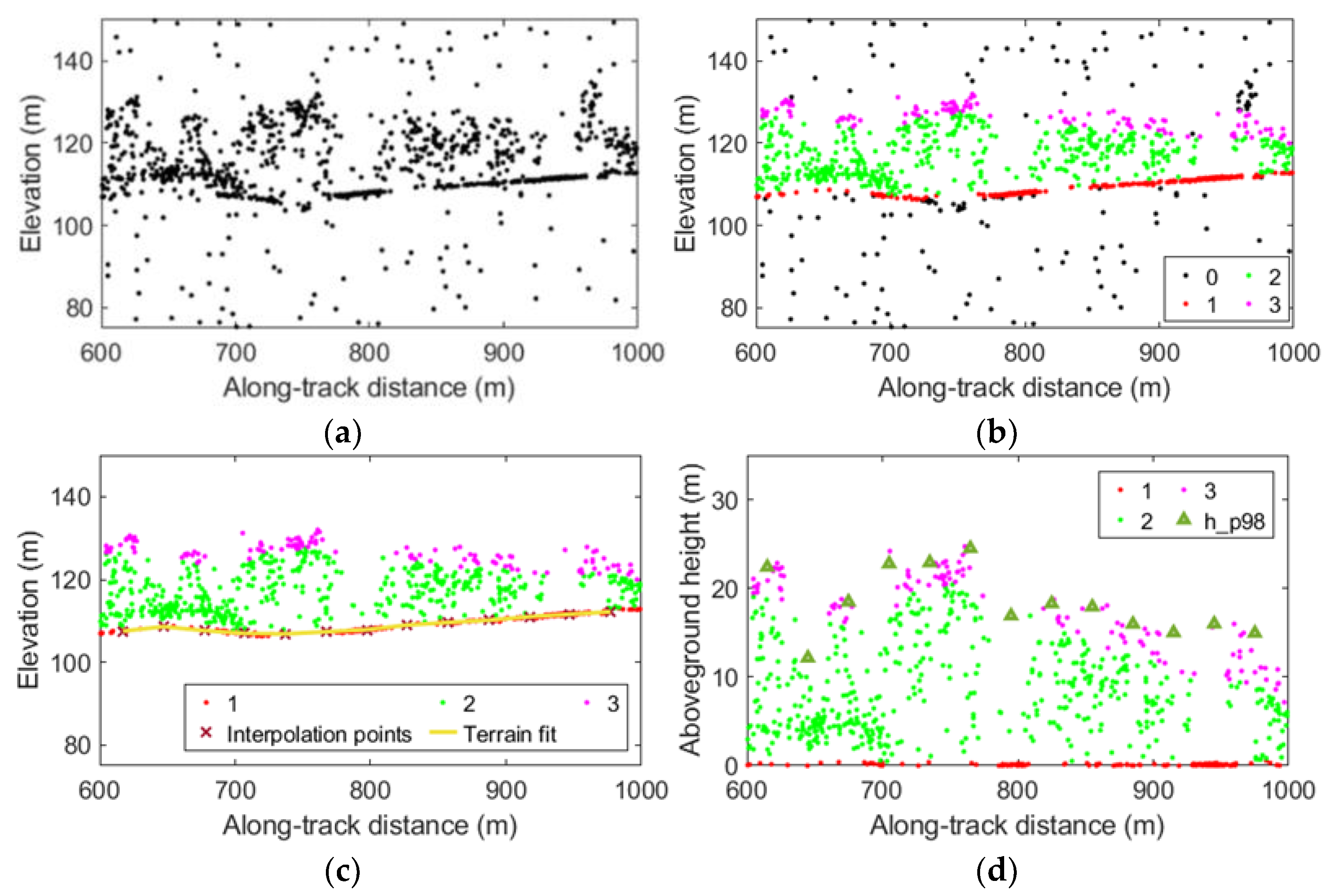
Our first processing step to derive classified point clouds involved matching ATL08 photon-level class values with corresponding ATL03 (Figure 2) values. This process involved matching each ATL08 photon classification index, that indicates the photon class (noise, terrain, canopy, and top of canopy), to a corresponding ATL03 point by linking common attributes such as the segment identification, spacecraft orbit, and cycles numbers [29]. While ATL08 processing routines provide adequate photon classification outputs, their retrieval accuracies are impacted by elevated levels of background noise and atmospheric interference from clouds and aerosols. Thus, in deriving the classified point clouds, we also extracted corresponding processing flags that codify these interferences and included them to enable post-filtering of bad data. These processing flags included: (1) the cloud confidence flag, which indicates the number of cloud or aerosol layers identified in each 25 Hz atmospheric profile; and (2) the multiple scattering warning flag, which indicates multiple atmospheric scattering [29]. Values greater than zero for each flag indicate presence of aerosols or clouds.

2.4.3. ICESat-2 Canopy Height Calculation

We estimated canopy height from classified photon data in 30-m segment lengths along each track in a ATL03 file. As a first step, we extracted terrain points from the classified points and binned the elevation values in 10 m interval along the track to fit a smooth curve through them. With a fitted terrain surface curve, we normalized the point clouds to aboveground level by subtracting the terrain surface elevation, the fitted curve, from all the data points (Figure 2c,d). From the aboveground data, we estimated canopy height as the 98th percentile of all heights within each 30 m segment, limiting the minimum number of points for a valid canopy height estimate to eleven. The ATL08 product calculates heights with at least 5% of canopy points in a 100-m segment. We thought 11 points were a conservative threshold for a 30-m segment. We processed all downloaded ICESat-2 data regardless of beam strength or time of acquisition to increase the amount of data for modeling.

2.4.4. Data Filtering and Sampling

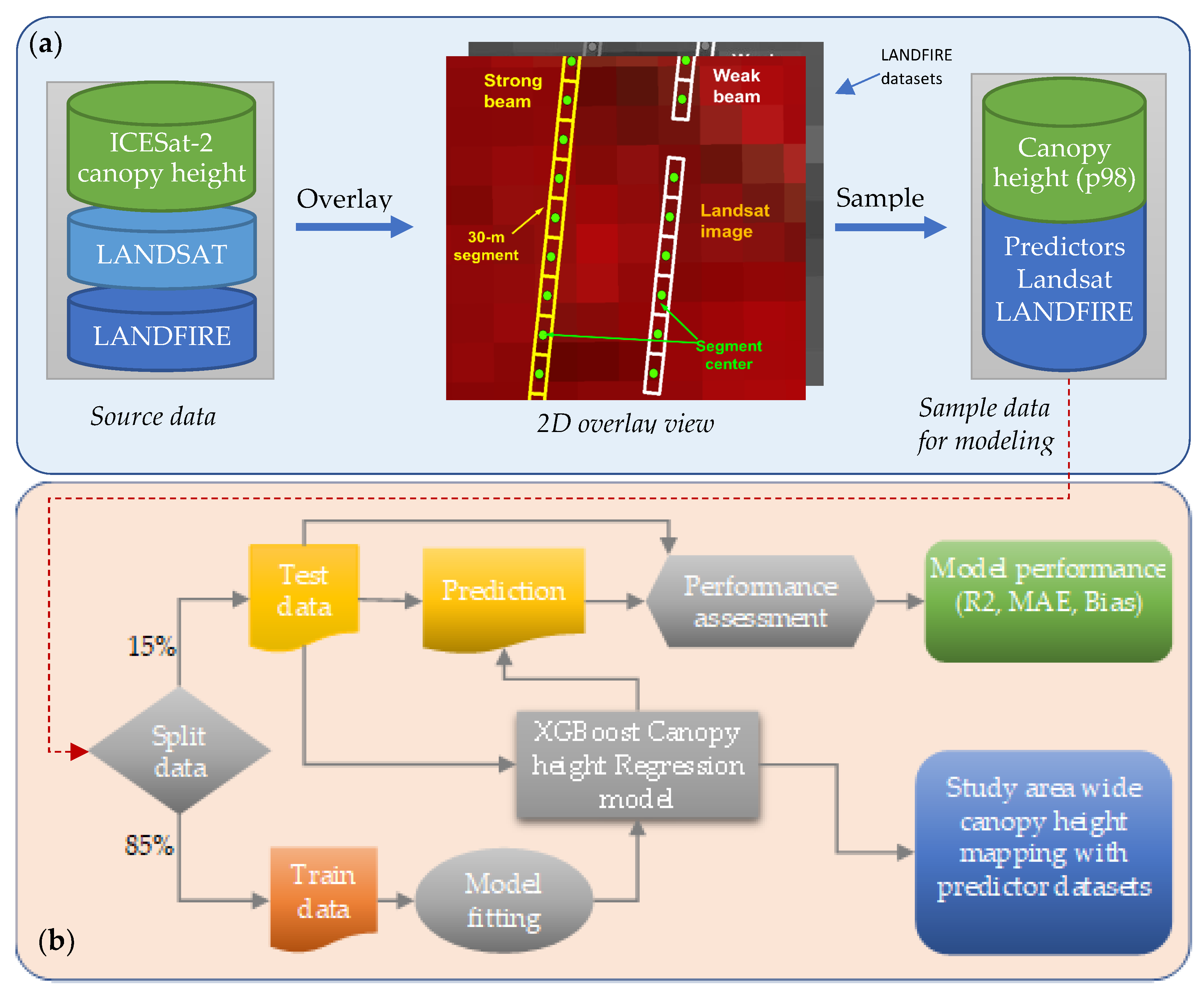
We gathered all the ICESat-2 canopy height estimates from each of the four sites to prepare data for analysis. To minimize the impacts of atmospheric factors, we filtered calculated canopy heights to enhance the quality of the estimates based on a priori knowledge and ATL08 processing flags (Section 2.4.2). First, we removed canopy heights greater than 60 m based on a priori knowledge of canopy height distribution over the study area. Further, we filtered out canopy heights based on the atmospheric processing flags. Following [30], we removed any canopy height estimate with a multiple scattering warning flag greater than zero and cloud confidence flag greater than one. All remaining ICESat-2 canopy height points were spatially overlaid on Landsat and LANDFIRE imagery to extract corresponding predictor values from the Landsat and LANDFIRE datasets, accounting for disturbance state and land cover (forest vs non-forest), to provide data for canopy height modeling (Figure 3a). Finally, a random sample (n = 23017) was selected from the compiled dataset to facilitate regression modeling as outlined in the following section.

2.5. Canopy Height Regression Modeling

2.5.1. Model Fitting and Evaluation

We developed regression models relating ICESat-2-derived canopy height with Landsat and LANDFIRE predictor variables using non-parametric gradient boosted regression trees implemented in the XGBoost library [31]. XGBoost, for Extreme Gradient Boosting, is an optimized distributed gradient boosting library which provides a parallel tree boosting to solve both classification and regression problems in a fast and accurate way. Unlike tree bagging based approaches, such as Random forests [32] that build multiple decision trees independently, XGBoost builds decision trees in a sequential way providing opportunities for incremental improvements during model fitting. In preliminary analyses to select a regression approach in this study, other algorithms were evaluated including Random Forests. XGBoost showed better performance and was subsequently adopted as the main method for this study.
In our preliminary analyses, models fitted with separate per-month Landsat and LANDFIRE showed lower performances against holdout data. Models build with Landsat showed R2 values ranging from 0.26 to 0.43 while a model build with only LANDFIRE variables showed R2 value of 0.48 (See Appendix A). Based on these preliminary results, the focus was to assess combinations of Landsat and LANDFIRE data for improved canopy height modeling. Thus, we evaluated three modeling combinations to assess the impact of using Landsat imagery acquired at various times during the year and to assess the benefit in combining multitemporal Landsat data. We set up regression models taking the ICESat-2 canopy height estimates as the dependent variable, and the Landsat images and LANDFIRE data as predictors using the following modeling combinations:
  • Separate models built using LANDFIRE data and each monthly Landsat image from January to December 2020.
  • A combined model built by combining all the Landsat 8 and LANDFIRE data to assess the benefit of using all the multitemporal Landsat data.
  • Reduced model built using LANDFIRE data and Landsat data from the four best performing months to assess if we could achieve a compromise between model performance and data volume.
For each of the models, we used 85% of the data for training and 15% for evaluating the accuracy of the prediction (Figure 3b). Performance metrics used for assessing each developed model include the coefficient of determination (R2), mean bias (Bias), mean absolute error (MAE), and their equivalent percent metrics, percent bias (pBias), and percent MAE (pMAE), as shown in Equations (1) through (5).
R   2 = ( n ( i = 1 n h i r i ) ( i = 1 n h i ) i = 1 n r i ) 2 [ n i = 1 n h i 2 ( i = 1 n h i ) 2 ] [ n i = 1 n r i 2 ( i = 1 n r i ) 2 ]
Bias = 1 n i = 1 n ( h i r i )
pBias = 100 × i = 1 n ( h i r i ) i = 1 n r i
MAE = 1 n i = 1 n | ( h i r i ) |
pMAE = 100 × i = 1 n | ( h i r i ) | i = 1 n r i
where hi is the ith predicted canopy height, ri is the ith reference canopy height, and n is the total number of samples used for the assessment. The coefficient of determination (R2) captured the correlation while the other metrics captured precision between predicted and reference canopy heights.
Assessing variable importance is an important step in machine learning modeling. For decision tree-based approaches such as gradient boosted trees, a variety of measures can be used including permutation, which measures the variable impact on model performance when its values are randomly permuted, or gain, which expresses the average improvement in model performance each time the variable is used in the trees. However, such measures tend to be biased toward often-used features and could provide inconsistent results [33]. SHAP (SHapley Additive exPlanations) values have been proposed as an alternative approach to enhance consistency and accuracy of variable importance assessment [33]. We adopted the approach in this study to assess each fitted model. The higher a calculated SHAP value is, the more important a variable is to overall model performance.

2.5.2. Scaling Along-Track Canopy Heights to a Regional Gridded Map

We produced a gridded canopy height product by applying the developed regression model to LANDFIRE and Landsat data over the study area. We selected a model developed from the model combinations outlined in Section 2.5.1 based on the prediction accuracy level and required data volume. The prediction of canopy height considered the land cover and disturbance state of each pixel, omitting (and set to zero) non-forest pixels, as defined from the EVT data, and changed pixels according to the disturbance data.
While we assessed model performance with holdout data, we were also interested in assessing the model generalization error over the study area. We compared the gridded canopy height product at a pixel level with canopy height models derived from airborne lidar in 35 1500 m by 1500 m randomly selected areas (Figure 1). We were also interested in comparing the generated product with existing canopy height datasets. One of the recently produced canopy height datasets is the GLAD global canopy height datasets (Table 1), hereafter the GLAD product. We conducted a three-way comparison involving airborne canopy height models, our gridded canopy height product, and the GLAD product disregarding non-forest and disturbed areas at each site.

3. Results

3.1. Canopy Height Regression Model Performance

Table 2 summarizes the performance of all models trained with different predictor combinations and evaluated on the 15% holdout data. Across the modeling scenarios, the R2 values ranged from 0.46 to 0.69 indicating moderate correlations with reference ICESat-2 canopy height estimates. On average, all the fitted models over-estimated the corresponding reference canopy heights by 0.04 m (average pBias = 0.25%). The MAE values ranged from 2.09 to 2.80 m which represent relative deviations from reference canopy heights of 10.8 to 14.5%. Model performance varied with the per-month Landsat data showing the impact of phenological changes on the modeling.
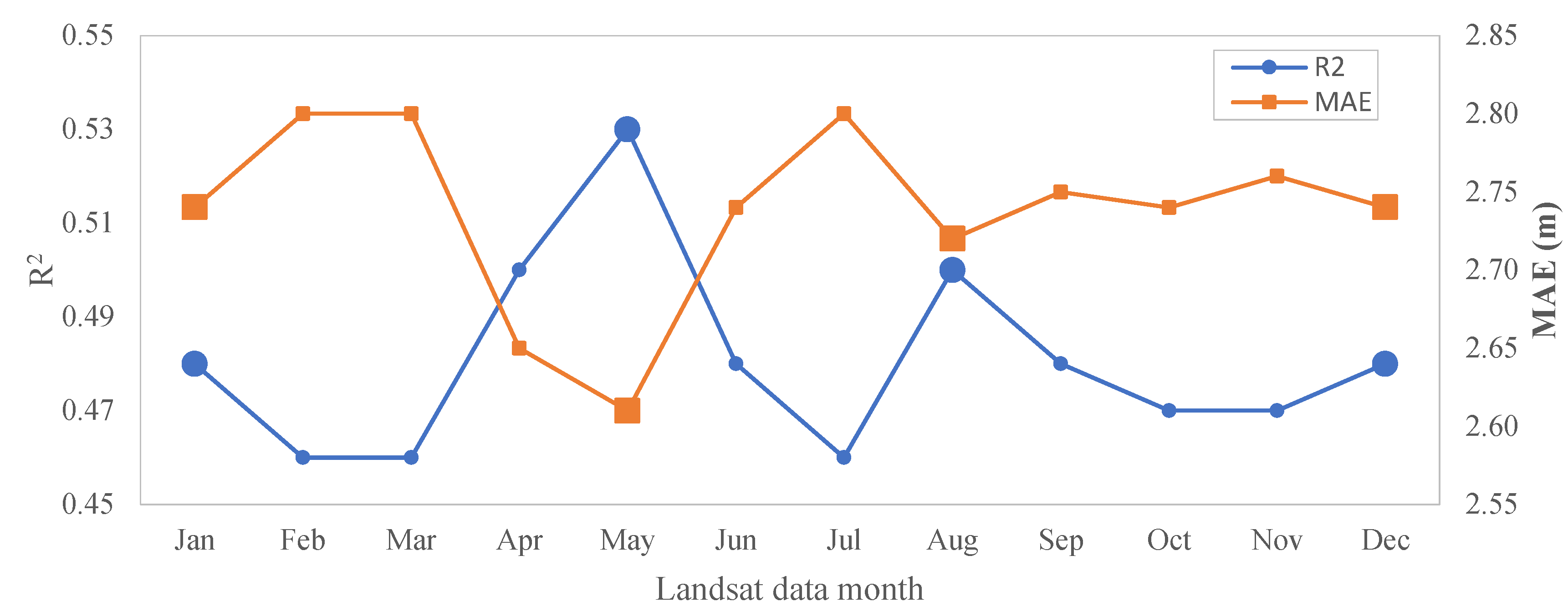
We observed a significant gain in model performance with the combined data—all Landsat and LANDFIRE—with an improvement in R2 of 43.5% and reduction in MAE of 23.7% on average. In an attempt to use fewer Landsat data, we also fit a reduced model (Best4; Table 2) using only the four best performing per-month Landsat data. We fit the Best4 model with the LANDFIRE data and Landsat data for January, May, August, and December, as these were the months that showed relative peaked performance (Figure 4), both in terms of correlation and precision, throughout the year. Using this reduced model still showed a significant improvement in performance with an improvement in R2 of 35.0% and reduction in MAE of 19.3% on average over models fit with individual Landsat data. While the combined model provided the better performance, the gain in precision over the Best4 model was not that significant. Thus, we considered the reduced (Best4) model a better compromise between model performance and data volume for generating the gridded canopy height product (Section 2.5.2 and Section 3.2).

3.2. Gridded Canopy Height Product and Assessment

We generated the gridded canopy height product over the study area by applying the reduced (Best4) model as we considered it a good compromise between performance and data volume. Figure 5a shows the output gridded canopy height product generated over the study area. The predicted canopy height ranged from 0 to 32.2 m with higher canopy heights (mean height = 21.1 m) falling around national forests dominated by pine species and along riparian areas where hardwood species like oaks are dominant. We observed lower canopy heights in the northern part of the region in East Central Texas forests characterized by more open forests and a greater concentration of hardwoods than the pines.
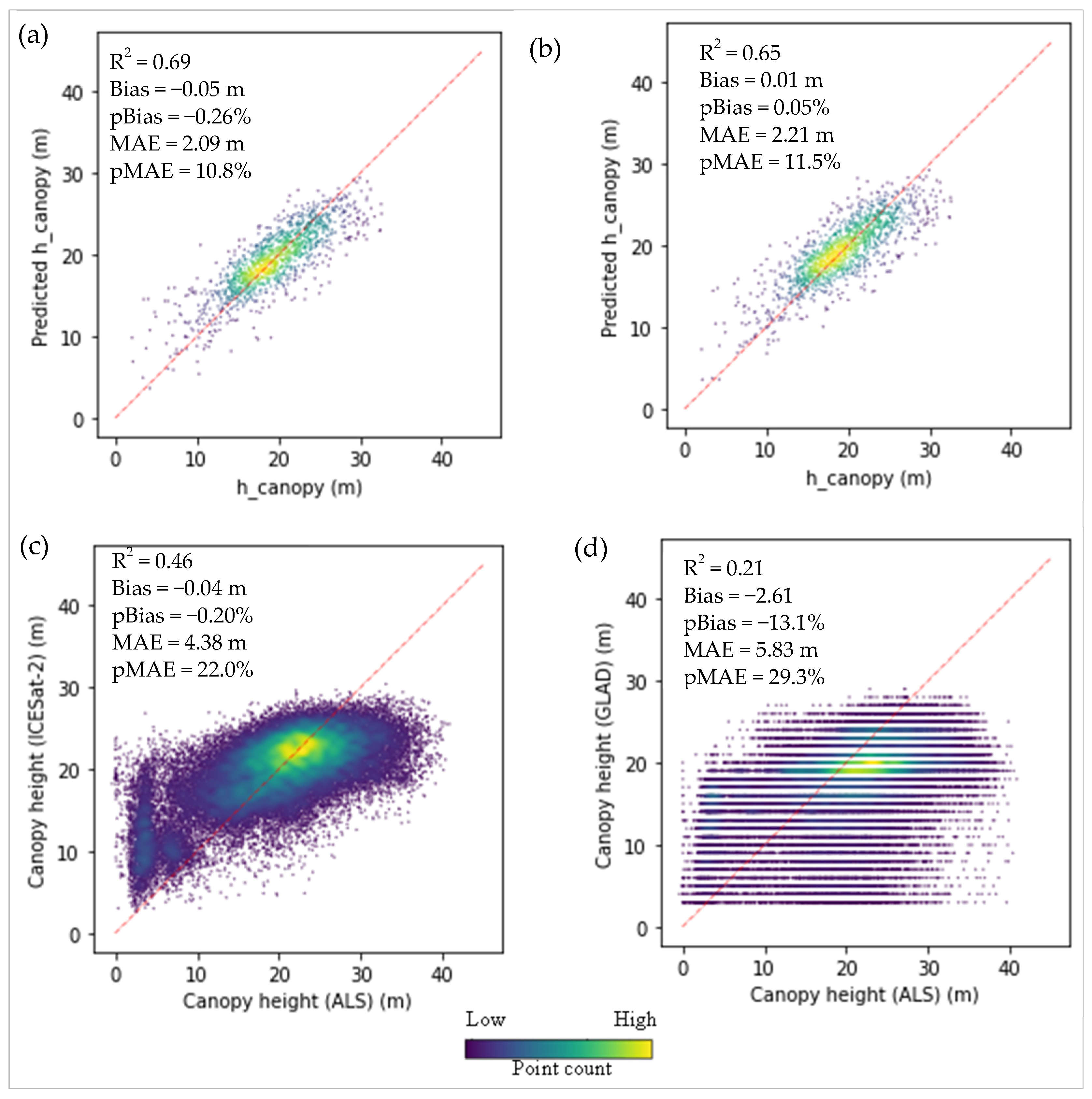
Our assessment of scaling performance over the entire study area using sample airborne lidar data showed fair agreement (R2 = 0.46, MAE = 4.38 m) with airborne lidar canopy height models (Figure 6c). As the scatter plots show (Figure 6a,b), there was a considerable amount of saturation in model predictions at the modeling stage compared to the levels observed, as evidenced by the increased lower predictions compared to airborne lidar heights. This error propagated to the generation of the gridded product as shown in Figure 6c. Our model also did not perform well for heights below 10 m, which could have been driven by the relative sparse sampling from ATLAS for shorter trees and lower canopy cover [5,30]. The tendency to saturate at higher forest heights or biomass levels when using reflectance-based predictors is also a well reported phenomenon, which is attributable to the fading correlation between forest structure and surface reflectance [34].
On the other hand, the comparison of the GLAD global canopy height product with airborne lidar canopy height models showed lower agreement (R2 = 0.19 MAE = 5.83 m) with reference heights derived from airborne lidar data (Figure 6d). Figure 5b,c show the GLAD product and its canopy height differences from our product. In general, GLAD canopy heights showed lower estimates compared to our product as can be seen from the green hue, a trend observed in other studies [10]. Where the two products differed by more than 5 m (represented by red color in Figure 5c), the pixels had undergone disturbance between 2018 and 2021. Thus, we suppose that the phenology-based modeling approach used in developing the GLAD product was inadequate in accounting for land cover changes.

4. Discussion

Spatially complete forest canopy height data are essential for terrestrial carbon modeling and studying forest structure dynamics [1]. With spaceborne lidar systems, we have the capability to estimate canopy height directly over large areas though limited to the predefined ground tracks. Optical imagery such as Landsat and derived datasets from the LANDFIRE program do not provide direct height measurement but offer the means to extend along-track canopy height estimates to provide spatially continuous coverage. In this study, we demonstrated that the fusion of these two sources can enable the production of spatially complete canopy height data over large areas. We assessed canopy height regression models at the modeling stage and also at the production level to assess the generalization of the models over the entire study area. Expectedly, fitted canopy height regression models performed better on holdout test data (R2 = 0.44–0.69, MAE = 2.14–2.77 m) than on selected reference canopy height models (R2 = 0.46, MAE = 4.38 m) as they represented mostly independent unseen data to the fitted model. Model performance in this study is generally consistent with previous studies (R2 = 0.5–0.7, RMSE = 4.2–6.1 m, MAE = 4.45–6.36 m) but some of them, e.g., [35], were produced at coarser spatial resolutions (500–1000 m) than ours. Given that aggregation at large spatial resolutions tend to favor better model fits [36], our results show reasonable improvement. Our results also show better modeling precision than similar studies [10,11] at the Landsat scale. We attribute these promising results to the XGBoost boosted trees model, which has demonstrated an effectiveness at modeling non-linear relationships in multidimensional space, and application of existing LANDFIRE datasets with a more direct correlation with the forest canopy structure.
Our product showed a better correlation to airborne lidar heights than the GLAD product. However, the differences in how the two products were produced could have confounded our assessments. The first factor relates to the differences between the canopy height metrics used. We used the 98th percentile to provide a canopy height estimate closer to the maximum canopy height and to be consistent with the ATL08 product definition of canopy height while the GLAD canopy height study used the 95th percentile height. Also, the GLAD study estimated canopy height as the median of predictions from an ensemble bagged trees model, which biased estimates toward lower values [11]. These factors explain the lower estimations from the GLAD product compared to ours. Also, the method of targeting forested areas differed for the two studies. The GLAD study targeted forest areas by using the 2010 existing tree cover product [11]. Given the extended period between 2010 and 2018 (acquisition year for GEDI and ICESat-2), it is conceivable that they did not effectively account for land cover changes. In our study, we applied a newer product from the 2016 LANDFIRE product, which shows a more recent reflection of existing forest cover. This effect was evidenced by large positive differences between ours and the GLAD product (Figure 5c). Other confounding factors include the geolocation uncertainties of GEDI versus ICESat-2, their relationship to airborne lidar and inherent differences in the pattern of ground coverage and sampling of canopy heights with waveform (GEDI) and photon-counting (ICESat-2) data.
Our modeling scenarios highlight well-known but critical structural and data-related factors for canopy height modeling. Vegetation phenology is a critical consideration when choosing Landsat images in a year for canopy height modeling as demonstrated by the varying model performance with per-month Landsat data (Figure 4). The best performance observed in April and May, leaf-on months in eastern Texas, was reflective of the stronger vegetation spectral signal and correlation with canopy height. However, our analyses showed that significant gains in modeling performance are achievable by combining multitemporal data (Table 2). Combining multitemporal data mimics sampling the vegetation phenology trends within one year, which enhances the vegetation signal but also the discrimination of vegetation of varying structures and species type [37]. However, using multitemporal data brings the practical challenges of high data volume and processing load, unless one has invested in high-performance or cloud-based computing resources. We showed that a reduced model built with fewer images in a year could provide a good balance between model performance and data volume.
Our assessment of variable importance for the combined and reduced model showed that near-infrared surface reflectance data, variables prefixed by b4, were among the most significant predictors in our modeling (Figure 7). This finding is important in the context of scaling up to the global canopy height characterization with Landsat imagery, when data products such as LANDFIRE are not available. The higher ranking of b4 data from three of the images used in the Best4 model also highlight the need to use data from different seasons. LANDFIRE predictors such as CH, CC, and EVH were among the higher-ranked features, but under-performed given their direct relationship to canopy height. The changes in vegetation structure (growth since 2016) as well as errors in production likely reduced their predictive power. It is worth noting that additional Landsat-derived variables such as spectral indices, principal components, and tasseled cap indices are variables that could have been incorporated in the modeling. Additional feature engineering using a combination of variables is another option that may supply more features for improved modeling [38]. For this case study, the goal of mapping canopy height was largely met with only individual spectral bands.
Our modeling framework relied on ATL08 photon-level classification data which enable the estimation of canopy heights consistent with the ancillary datasets. The main drawback here is that ATL08 photon-level classification data contain varying levels of misclassification error. Given that the reliable estimation of canopy height requires an accurate photon classification, such errors need to be minimized to derive valid canopy height estimates. In this study, we visually inspected the ICESat-2 data to remove bad data using the PhotonLabeler application [24], which was adequate for choosing input data for modeling. However, using such an approach is tedious and would not meet large scale analyses especially where spatial interpolation approaches are considered. This challenge presents opportunities to develop reprocessing algorithms to increase the quality of ATL08 photon classifications. Such research endeavors would enable the production of analysis-ready point cloud datasets that would support a wider array of end uses than currently offered. Further research is also needed to guide users in detecting and removing problematic ATL08 height estimates. Limited research exists on the use of quality flags in the ATL08 product to enable the automated characterization of bad data granules. A related issue concerns the level of sampling achieved by the ICESat-2 sensor. ICESat-2 records only 0–4 photons from an emitted laser pulse over vegetation surfaces [23], which could lead to inadequate characterization of canopy tops. This effect in part explains the increased under-estimation of airborne lidar heights (Figure 6c).
While this study focused on eastern Texas, the modeling framework developed here presents an opportunity to extend canopy height mapping to other regions across the contiguous United States as datasets applied are available at a national scale under a consistent processing methodology. As canopy height is a vital input to carbon modeling, canopy products as generated in this study offer possibilities for the regional monitoring of carbon stocks [2]. It is also possible to extend this analysis framework to other years to facilitate the monitoring of the status and trends in forest resources. ICESat-2 will continue to orbit and densify the sampling of the Earth, providing more elevation observations to support even more accurate products that those generated at this time. Just like the multisource approach enabled the generation of the gridded canopy height product, there is the chance to reinforce it by combining it with other spaceborne lidar data such as that from the GEDI mission. Work in the direction has already been demonstrated by a number of studies for canopy height [10] and biomass estimation [39], providing a stronger foundation for collecting information on the three-dimensional vegetation structure from space.

5. Conclusions

In this study, we demonstrated the fusion of spaceborne elevation measurements from ICESat-2 mission and ancillary Landsat and LANDFIRE data for the development of a spatially complete regional canopy height product at a 30 m Landsat scale. Our modeling showed canopy height predictions with moderate to high correlation and showed moderate precision compared to reference canopy heights, showing adequate consistency in the developed models. Our analyses also showed that canopy height with Landsat data from a single month does not provide adequate performance but significant gains in performance are achievable with multiple Landsat images across the year. Both Landsat and LANDFIRE predictors contributed to the model performance but the Landsat near-infrared surface reflectance was the best-ranked variable across modeling combinations. While only spectral bands were applied in this case study, there is room for derived variables such as spectral indices, principal components, and tasseled cap indices to improve canopy height modeling and wall-to-wall mapping. The inclusion of these variables could also enable the application of the modeling framework presented in this study to regions outside the United States that do not have LANDFIRE datasets.
The canopy height product generated with the developed regression models showed a moderate correlation with airborne lidar canopy heights, thus indicating the developed models scaled generally well across the study area. However, the canopy height product showed lower agreement with airborne lidar canopy heights for height values below 10 m, which we attribute to inadequacies in sampling from the ATLAS instrument for shorter trees and lower canopy cover. Given that the reliable estimation of canopy height requires an accurate photon classification, errors due to photon misclassifications could also have contributed to the reduced performance. We recommend denser and spatially more balanced sampling to alleviate the scaling issues for future studies. Our canopy height product showed disagreement with the GLAD canopy height dataset mainly in areas mapped as disturbed, which we supposed were not adequately accounted for in the GLAD. Ultimately, our product showed better agreement with airborne lidar heights when samples from undisturbed areas were assessed.
While there is still room for improvement in the modeling and scaling of ICESat-2 along-track ICESat-2 heights, this study presented a viable framework for mapping canopy heights at large scales with height data consistent with ancillary data spatial resolutions. Wall-to-wall coverage products as generated in this study provide a valuable spatially detailed and synoptic view of canopy heights over the study area, which would support improved targeting areas for timber harvest, carbon accounting, and ecological process assessments at a 30 Landsat spatial resolution.

Author Contributions

Conceptualization, L.M.; Methodology, L.M. and S.P.; Software, L.M.; Validation, L.M. and M.L.; Formal analysis, L.M.; Investigation, L.M.; Data curation, L.M. and M.L.; Writing–original draft, L.M. and S.P.; Writing–review & editing, L.M.; Visualization, L.M.; Funding acquisition, L.M. and S.P. All authors have read and agreed to the published version of the manuscript.

Funding

This research was supported by an International Paper Research Grants—Forest Sustainability grant, and by funding from the NASA ICESat-2 Science Team, Studies with ICESat-2 (NNH19ZDA001N) grant.

Data Availability Statement

Publicly available datasets were analyzed in this study. These data can be found using links provided in the paper.

Conflicts of Interest

The authors declare that they have no known competing financial interests or personal relationships that could have appeared to influence the work reported in this paper.

Appendix A

This section highlights preliminary analyses conducted to evaluate ICESat-2 canopy height regression model performance with separate per-month Landsat and LANDFIRE variables against holdout data. The following table (Table A1) summarizes the results obtained from the various model fits using the same modeling approach as depicted in Figure 3b.
Table A1. Model performance summary based on the 15% holdout data (n = 3453).
Per-Month Landsat VariablesLANDFIRE
JanFebMarAprMayJunJulAugSepOctNovDec
R20.430.390.260.360.430.370.320.390.340.420.390.420.48
Bias (m)−0.01−0.050.010.04−0.01−0.0400.01−0.08−0.040.050.01−0.05
pBias (%)−0.06−0.210.050.16−0.02−0.170.020.05−0.35−0.210.250.04−0.21
MAE (m)3.553.714.093.743.513.743.933.73.893.623.713.613.37
pMAE (%)16.5417.2719.0617.416.3517.4118.2717.2418.1116.8517.2816.8315.67

References

  1. Schimel, D.; Pavlick, R.; Fisher, J.B.; Asner, G.P.; Saatchi, S.; Townsend, P.; Miller, C.; Frankenberg, C.; Hibbard, K.; Cox, P. Observing terrestrial ecosystems and the carbon cycle from space. Glob. Chang. Biol. 2015, 21, 1762–1776. [Google Scholar] [CrossRef] [PubMed]
  2. Radtke, P.; Walker, D.; Frank, J.; Weiskittel, A.; DeYoung, C.; MacFarlane, D.; Domke, G.; Woodall, C.; Coulston, J.; Westfall, J. Improved accuracy of aboveground biomass and carbon estimates for live trees in forests of the eastern united states. For. Int. J. For. Res. 2017, 90, 32–46. [Google Scholar] [CrossRef] [Green Version]
  3. Nelson, R.; Valenti, M.A.; Short, A.; Keller, C. A multiple resource inventory of delaware using airborne laser data. Bioscience 2003, 53, 981–992. [Google Scholar] [CrossRef] [Green Version]
  4. Wulder, M.A.; White, J.C.; Nelson, R.F.; Næsset, E.; Ørka, H.O.; Coops, N.C.; Hilker, T.; Bater, C.W.; Gobakken, T. Lidar sampling for large-area forest characterization: A review. Remote Sens. Environ. 2012, 121, 196–209. [Google Scholar] [CrossRef] [Green Version]
  5. Malambo, L.; Popescu, S.C. Assessing the agreement of icesat-2 terrain and canopy height with airborne lidar over us ecozones. Remote Sens. Environ. 2021, 266, 112711. [Google Scholar] [CrossRef]
  6. Markus, T.; Neumann, T.; Martino, A.; Abdalati, W.; Brunt, K.; Csatho, B.; Farrell, S.; Fricker, H.; Gardner, A.; Harding, D.; et al. The ice, cloud, and land elevation satellite-2 (icesat-2): Science requirements, concept, and implementation. Remote Sens. Environ. 2017, 190, 260–273. [Google Scholar] [CrossRef]
  7. Magruder, L.A.; Brunt, K.M.; Alonzo, M. Early icesat-2 on-orbit geolocation validation using ground-based corner cube retro-reflectors. Remote Sens. 2020, 12, 3653. [Google Scholar] [CrossRef]
  8. Neumann, T.; Brenner, A.; Hancock, D.; Robbins, J.; Saba, J.; Harbeck, K.; Gibbons, A. Ice, Cloud, and Land Elevation Satellite–2 (Icesat-2) Project: Algorithm Theoretical Basis Document (Atbd) for Global Geolocated Photons (atl03); National Aeronautics and Space Administration, Goddard Space Flight Center: Greenbelt, MD, USA, 2019.
  9. Popescu, S.C.; Zhou, T.; Nelson, R.; Neuenschwander, A.; Sheridan, R.; Narine, L.; Walsh, K.M. Photon counting lidar: An adaptive ground and canopy height retrieval algorithm for icesat-2 data. Remote Sens. Environ. 2018, 208, 154–170. [Google Scholar] [CrossRef]
  10. Liu, X.; Su, Y.; Hu, T.; Yang, Q.; Liu, B.; Deng, Y.; Tang, H.; Tang, Z.; Fang, J.; Guo, Q. Neural network guided interpolation for mapping canopy height of China’s forests by integrating gedi and icesat-2 data. Remote Sens. Environ. 2022, 269, 112844. [Google Scholar] [CrossRef]
  11. Potapov, P.; Li, X.; Hernandez-Serna, A.; Tyukavina, A.; Hansen, M.C.; Kommareddy, A.; Pickens, A.; Turubanova, S.; Tang, H.; Silva, C.E.; et al. Mapping global forest canopy height through integration of gedi and landsat data. Remote Sens. Environ. 2021, 253, 112165. [Google Scholar] [CrossRef]
  12. Simard, M.; Pinto, N.; Fisher, J.B.; Baccini, A. Mapping forest canopy height globally with spaceborne lidar. J. Geophys. Res. Biogeosci. 2011, 116, G04021. [Google Scholar] [CrossRef] [Green Version]
  13. Ghamisi, P.; Rasti, B.; Yokoya, N.; Wang, Q.; Hofle, B.; Bruzzone, L.; Bovolo, F.; Chi, M.; Anders, K.; Gloaguen, R. Multisource and multitemporal data fusion in remote sensing: A comprehensive review of the state of the art. IEEE Geosci. Remote Sens. Mag. 2019, 7, 6–39. [Google Scholar] [CrossRef] [Green Version]
  14. Lunetta, R.S.; Johnson, D.M.; Lyon, J.G.; Crotwell, J. Impacts of imagery temporal frequency on land-cover change detection monitoring. Remote Sens. Environ. 2004, 89, 444–454. [Google Scholar] [CrossRef]
  15. Kennedy, R.E.; Yang, Z.; Gorelick, N.; Braaten, J.; Cavalcante, L.; Cohen, W.B.; Healey, S. Implementation of the landtrendr algorithm on google earth engine. Remote Sens. 2018, 10, 691. [Google Scholar] [CrossRef] [Green Version]
  16. Montesano, P.; Rosette, J.; Sun, G.; North, P.; Nelson, R.; Dubayah, R.; Ranson, K.; Kharuk, V. The uncertainty of biomass estimates from modeled icesat-2 returns across a boreal forest gradient. Remote Sens. Environ. 2015, 158, 95–109. [Google Scholar] [CrossRef]
  17. Liu, M.; Popescu, S.; Malambo, L. Effects of spatial resolution on burned forest classification with icesat-2 photon counting data. Front. Remote Sens. 2021, 17, 666251. [Google Scholar] [CrossRef]
  18. Malambo, L.; Popescu, S.C.; Murray, S.C.; Putman, E.; Pugh, N.A.; Horne, D.W.; Richardson, G.; Sheridan, R.; Rooney, W.L.; Avant, R.; et al. Multitemporal field-based plant height estimation using 3d point clouds generated from small unmanned aerial systems high-resolution imagery. Int. J. Appl. Earth Obs. Geoinf. 2018, 64, 31–42. [Google Scholar] [CrossRef]
  19. Vogelmann, J.E.; Xian, G.; Homer, C.; Tolk, B. Monitoring gradual ecosystem change using landsat time series analyses: Case studies in selected forest and rangeland ecosystems. Remote Sens. Environ. 2012, 122, 92–105. [Google Scholar] [CrossRef] [Green Version]
  20. Rollins, M.G. Landfire: A nationally consistent vegetation, wildland fire, and fuel assessment. Int. J. Wildland Fire 2009, 18, 235–249. [Google Scholar] [CrossRef] [Green Version]
  21. Elliott, L. Descriptions of Systems, Mapping Subsystems, and Vegetation Types for Texas. In Texas Parks and Wildlife Ecological Systems Classification and Mapping Project; Texas Parks & Wildlife Department: Austin, TX, USA, 2014. [Google Scholar]
  22. Dinerstein, E.; Olson, D.; Joshi, A.; Vynne, C.; Burgess, N.D.; Wikramanayake, E.; Hahn, N.; Palminteri, S.; Hedao, P.; Noss, R.; et al. An ecoregion-based approach to protecting half the terrestrial realm. Bioscience 2017, 67, 534–545. [Google Scholar] [CrossRef]
  23. Neuenschwander, A.; Pitts, K. The atl08 land and vegetation product for the icesat-2 mission. Remote Sens. Environ. 2019, 221, 247–259. [Google Scholar] [CrossRef]
  24. Malambo, L.; Popescu, S. Photonlabeler: An inter-disciplinary platform for visual interpretation and labeling of icesat-2 geolocated photon data. Remote Sens. 2020, 12, 3168. [Google Scholar] [CrossRef]
  25. Moreno-Martínez, Á.; Izquierdo-Verdiguier, E.; Maneta, M.P.; Camps-Valls, G.; Robinson, N.; Muñoz-Marí, J.; Sedano, F.; Clinton, N.; Running, S.W. Multispectral high resolution sensor fusion for smoothing and gap-filling in the cloud. Remote Sens. Environ. 2020, 247, 111901. [Google Scholar] [CrossRef] [PubMed]
  26. Malambo, L.; Heatwole, C.D. Automated training sample definition for seasonal burned area mapping. ISPRS J. Photogramm. Remote Sens. 2020, 160, 107–123. [Google Scholar] [CrossRef]
  27. Malambo, L.; Heatwole, C.D. A multitemporal profile-based interpolation method for gap filling nonstationary data. IEEE Trans. Geosci. Remote Sens. 2015, 54, 252–261. [Google Scholar] [CrossRef]
  28. Thatcher, C.A.; Lukas, V.; Stoker, J.M. The 3D Elevation Program and Energy for the Nation; US Geological Survey: Reston, VA, USA, 2020; pp. 2327–6932. [Google Scholar]
  29. Neuenschwander, A.; Pitts, K.; Jelley, B.; Robbins, J.; Klotz, B.; Popescu, S.; Nelson, R.; Harding, D.; Pederson, D.; Sheridan, R. Atlas/Icesat-2 l3a Land and Vegetation Height, Version 5; NSIDC: National Snow and Ice Data Center: Boulder, CO, USA, 2021. [Google Scholar]
  30. Neuenschwander, A.; Guenther, E.; White, J.C.; Duncanson, L.; Montesano, P. Validation of icesat-2 terrain and canopy heights in boreal forests. Remote Sens. Environ. 2020, 251, 112110. [Google Scholar] [CrossRef]
  31. Chen, T.; He, T.; Benesty, M.; Khotilovich, V.; Tang, Y.; Cho, H. Xgboost: Extreme gradient boosting. R Package Version 0.4-2 2015, 1, 1–4. [Google Scholar]
  32. Breiman, L. Random forests. Mach. Learn. 2001, 45, 5–32. [Google Scholar] [CrossRef] [Green Version]
  33. Lundberg, S.M.; Lee, S.-I. A unified approach to interpreting model predictions. Adv. Neural Inf. Process. Syst. 2017, 30, 4768–4777. [Google Scholar]
  34. Wijaya, A.; Kusnadi, S.; Gloaguen, R.; Heilmeier, H. Improved strategy for estimating stem volume and forest biomass using moderate resolution remote sensing data and gis. J. For. Res. 2010, 21, 1–12. [Google Scholar] [CrossRef]
  35. Lefsky, M.A. A global forest canopy height map from the moderate resolution imaging spectroradiometer and the geoscience laser altimeter system. Geophys. Res. Lett. 2010, 37. [Google Scholar] [CrossRef] [Green Version]
  36. Blackard, J.; Finco, M.; Helmer, E.; Holden, G.; Hoppus, M.; Jacobs, D.; Lister, A.; Moisen, G.; Nelson, M.; Riemann, R. Mapping us forest biomass using nationwide forest inventory data and moderate resolution information. Remote Sens. Environ. 2008, 112, 1658–1677. [Google Scholar] [CrossRef]
  37. Huang, C.; Coward, S.N.; Masek, J.G.; Thomas, N.; Zhu, Z.; Vogelmann, J.E. An automated approach for reconstructing recent forest disturbance history using dense landsat time series stacks. Remote Sens. Environ. 2010, 114, 183–198. [Google Scholar] [CrossRef]
  38. Horn, F.; Pack, R.; Rieger, M. The Autofeat Python Library for Automated Feature Engineering and Selection. In Joint European Conference on Machine Learning and Knowledge Discovery in Databases, 2019; Springer: Berlin/Heidelberg, Germany, 2019; pp. 111–120. [Google Scholar]
  39. Silva, C.A.; Duncanson, L.; Hancock, S.; Neuenschwander, A.; Thomas, N.; Hofton, M.; Fatoyinbo, L.; Simard, M.; Marshak, C.Z.; Armston, J. Fusing simulated gedi, icesat-2 and nisar data for regional aboveground biomass mapping. Remote Sens. Environ. 2021, 253, 112234. [Google Scholar] [CrossRef]
Figure 1. Study area in eastern Texas, USA showing ecoregion coverage [22], ICESat-2 data sampling sites and distribution of reference airborne lidar data. Topographic base maps courtesy of ESRI ArcGIS®.
Remotesensing 15 00001 g001
Figure 2. Calculating canopy heights in 30-m segments. (a) Raw ATL03 point cloud rendered a 2D plot of along-track distance against elevation, (b) Classified point cloud derived by linking ATL08 photon classifications with ATL03 point cloud, (c) Removal of noise points and terrain curve fitting to support aboveground point cloud normalization, (d) Canopy height estimated as 98th percentile height (h_p98) overlaid on normalized point cloud.
Remotesensing 15 00001 g002
Figure 3. (a) Data overlay and sampling. The middle element in the figure illustrates the custom 30-m segments overlaid on a sample Landsat/LANDFIRE image stack and extraction of corresponding predictor data, (b) Schematic workflow for canopy height modeling and wall to wall mapping across the study area.
Remotesensing 15 00001 g003
Figure 4. Per-month variation in canopy height modeling performance with relative peaked performance for Jan, May, Aug, and Dec symbolized by larger markers. Each model was trained with a per-month Landsat data and LANDFIRE variables.
Remotesensing 15 00001 g004
Figure 5. (a) Generated gridded canopy height product, (b) GLAD canopy height product, (c) Differences between the two products.
Remotesensing 15 00001 g005
Figure 6. Scatter plot of predicted vs reference canopy height in meters: (a) Model performance on holdout test data using LANDFIRE and combined monthly Landsat data, (b) Model performance on holdout test data using LANDFIRE and best four monthly Landsat data, (c) Performance of generated canopy height map against airborne lidar canopy heights, (d) Performance of GLAD product against airborne lidar canopy heights.
Remotesensing 15 00001 g006
Figure 7. Variable importance for combined (a) and reduced (b) canopy regression models for the best 30 features. Features starting with a ‘b’ represent Landsat bands with respective month abbreviations. LANDFIRE variables include EVH, CH, CBH, CC, and CBD.
Remotesensing 15 00001 g007
Table 1. List of ancillary and accuracy assessment datasets applied in the study.
DatasetDescription and Purpose
2020 Monthly Gap-filled Landsat data 2020 Monthly gap-filled Landsat data produced by fusing Landsat and MODIS multispectral images [25]. Source: Google Earth Engine (https://code.earthengine.google.com/?asset=projects/KalmanGFwork/GFLandsat_V1 (accessed on 20 August 2022)).
2020 LANDFIRE Existing Vegetation Height (EVH)The average height of the dominant vegetation for a 30-m grid cell.
2020 LANDFIRE Forest Canopy Height (CH)The average height of the top of the vegetated canopy a 30-m grid cell. Estimated in forested areas only.
2020 LANDFIRE Forest Canopy Base Height (CBH)The average height from the ground to a forest stand’s canopy bottom.
2020 LANDFIRE Forest Canopy Cover (CC)Percent tree cover, estimated in forested areas only. Values range from 15 to 95% in 10% steps. Non-forest assigned value 0.
2020 LANDFIRE Forest Canopy Bulk Density (CBD)The density of available canopy fuel in a stand, estimated in forested areas only. For ancillary forest structure information.
2020 LANDFIRE Existing Vegetation Type (EVT)Represents mapped current distribution of the terrestrial ecological systems classification.
Land cover disturbance 2016–2021Binary land cover change layer indicating areas that changed from 2016 as mapped by LandTrendr algorithms. Processing script adapted from: https://emapr.github.io/LT-GEE/example-scripts.html (accessed on 20 August 2022)
Airborne lidar data (2016–2018)Source of canopy height validation data. Refer to Figure 1 for spatial distribution of the data collected.
Global Land Analysis and Discovery (GLAD) GEDI Global Forest Canopy Height, 2019Existing canopy height dataset for comparative assessment with our generated product. Data is available at the GLAD website (https://glad.umd.edu/dataset/gedi/ (accessed on 16 October 2022)) or through a Google Earth Engine Application (https://glad.earthengine.app/view/global-forest-canopy-height-2019 (accessed on 16 October 2022)).
Table 2. Model performance summary based on the 15% holdout data (n = 3453). Per-month modeling combinations e.g., Jan, represent the model trained with January Landsat image and LANDFIRE variables. Best4 is the reduced model while All is the model trained with all Landsat images in the year and LANDFIRE variables.
JanFebMarAprMayJunJulAugSepOctNovDecBest4All
R20.480.460.460.500.530.480.460.500.480.470.470.480.650.69
Bias (m)0.040.030.050.080.010.060.100.050.000.050.060.050.01−0.05
pBias (%)0.230.160.250.440.050.300.500.28−0.010.250.300.280.05−0.26
MAE (m)2.742.802.802.652.612.742.802.722.752.742.762.742.212.09
pMAE (%)14.214.514.513.713.514.214.514.114.214.214.314.211.510.8
Disclaimer/Publisher’s Note: The statements, opinions and data contained in all publications are solely those of the individual author(s) and contributor(s) and not of MDPI and/or the editor(s). MDPI and/or the editor(s) disclaim responsibility for any injury to people or property resulting from any ideas, methods, instructions or products referred to in the content.