Technical Note

Rossby Waves in Total Ozone over the Arctic in 2000–2021

1
International Center of Future Science, College of Physics, Jilin University, Changchun 130012, China
2
Physics Faculty, Taras Shevchenko National University of Kyiv, 01601 Kyiv, Ukraine
3
Department of Atmosphere Physics and Geospace, National Antarctic Scientific Center, 01601 Kyiv, Ukraine
4
Laboratoire d’Optique Atmosphérique, Département de Physique, Université de Lille, 59655 Villeneuve d’Ascq, France
5
Department of Millimeter Radio Astronomy, Institute of Radio Astronomy, National Academy of Sciences of Ukraine, 61002 Kharkiv, Ukraine
6
Antarctic Climate Program, Australian Antarctic Division, Kingston 7050, Australia
7
Department of Physics, University of Adelaide, Adelaide 5005, Australia
8
Space Radio-Diagnostics Research Centre, University of Warmia and Mazury in Olsztyn, 10-719 Olsztyn, Poland
9
Main Center of Special Monitoring, National Space Facilities Control and Test Center, State Space Agency of Ukraine, 01010 Kyiv, Ukraine
*
Author to whom correspondence should be addressed.
Remote Sens. 2022, 14(9), 2192; https://doi.org/10.3390/rs14092192
Submission received: 28 March 2022 / Revised: 1 May 2022 / Accepted: 2 May 2022 / Published: 4 May 2022
(This article belongs to the Section Atmospheric Remote Sensing)

Abstract

:
The purpose of this work is to study Rossby wave parameters in total ozone over the Arctic in 2000–2021. We consider the averages in the January–March period, when stratospheric trace gases (including ozone) in sudden stratospheric warming events are strongly disturbed by planetary waves. To characterize the wave parameters, we analyzed ozone data at the latitudes of 50°N (the sub-vortex area), 60°N (the polar vortex edge) and 70°N (inner region of the polar vortex). Total ozone column (TOC) measurements over a 22-year time interval were used from the Total Ozone Mapping Spectrometer/Earth Probe and Ozone Mapping Instrument/Aura satellite observations. The TOC zonal distribution and variations in the Fourier spectral components with zonal wave numbers m = 1–5 are presented. The daily and interannual variations in TOC, amplitudes and phases of the spectral wave components, as well as linear trends in the amplitudes of the dominant quasi-stationary wave 1 (QSW1), are discussed. The positive TOC peaks inside the vortex in 2010 and 2018 alternate with negative ones in 2011 and 2020. The extremely low TOC at 70°N in 2020 corresponds to severe depletion of stratospheric ozone over the Arctic in strong vortex conditions due to anomalously low planetary wave activity and a high positive phase of the Arctic Oscillation. Interannual TOC variations in the sub-vortex region at 50°N are accompanied by a negative trend of −4.8 Dobson Units per decade in the QSW1 amplitude, statistically significant at 90% confidence level, while the trend is statistically insignificant in the vortex edge region and inside the vortex due to the increased variability in TOC and QSW1. The processes associated with quasi-circumpolar migration and quasi-stationary oscillation of the wave-1 phase depending on the polar vortex strength in 2020 and 2021 are discussed.

1. Introduction

In winter, the structure of the Arctic stratosphere is dominated by the formation of a cyclonic cell known as the polar vortex [1,2]. The behavior of the vortex can be disturbed by large-scale Rossby waves propagating in its vicinity, and the amount of this disturbance varies significantly from season to season. In years when wave activity is weak, the stratospheric polar vortex can be very stable and last until mid-spring, as was the case in 2020 [3]. Under these conditions, the air inside the vortex becomes strongly isolated from the air masses of middle latitudes, while outside the vortex, ozone accumulates due to its transport from lower latitudes by the Brewer–Dobson circulation [4,5]. As winter progresses, radiative cooling in the polar night can trigger the large-scale formation of polar stratospheric clouds; heterogeneous reactions on the surface of the cloud particles then promote conditions suitable for the destruction of ozone molecules when sunlight returns in spring [6]. These conditions result in rapid ozone loss and the formation of ozone hole conditions, as occurred in the Artic during 2020 [7]. In contrast, under high Rossby wave activity the polar vortex is weak, and its ozone content at polar latitudes shows a seasonal maximum in spring analogous to that at mid-latitudes [8].
The ability of large-scale disturbances to propagate into the stratosphere is generally described by the Charney–Drazin criterion [9], which admits upward wave propagation for background westerly winds of a moderate velocity. The waves of most significance in disturbing the stratospheric polar vortex are those with zonal numbers 1 and 2, which are predominantly quasi-stationary and eastward moving, respectively [10]. These waves produce circulation anomalies that affect ozone transport. Because of the relatively long lifetime of the ozone molecule in the absence of heterogeneous reactions, these circulation anomalies and the characteristics of the governing wave activity can be effectively mapped through examination of total ozone column (TOC) measurements. Investigation of Rossby waves using synoptic TOC satellite measurements is slightly affected by the westward phase shift of the waves with altitude in the lower and middle stratosphere [11], where atmospheric ozone dominates [12].
The breaking of Rossby waves in the polar stratosphere results in rapid increases in temperature, known as sudden stratospheric warmings (SSWs; [13,14,15]). In the northern hemisphere, these events occur approximately every second winter. The stratospheric polar vortex during an SSW weakens, splits, or even terminates, which leads to the restoration of normal TOC levels. In the Northern Hemisphere, SSWs are observed from late November to late March [16], with most events occurring in January–February, while final warmings occur mainly in March and April, and rarely as late as mid-May [17,18].
The relationship between planetary wave activity and the distribution and variability of TOC has been studied using satellite observations since 1979 [4,8,11,19]. This paper considers the characteristics of Rossby waves in TOC over the Arctic region using satellite data over the past two decades (2000–2021). We focus our analysis on the months January–March, when SSWs mainly occur and trace gases in the Arctic stratosphere (including ozone) can be strongly disturbed [3,7,17]. To characterize the amplitudes and phases of the Rossby waves, we use the latitudes of 50°N (the sub-vortex area), 60°N and 70°N (edge and inner regions of the polar vortex, respectively). Below, in Section 2, we describe the data used and the analysis method. In Section 3, the total ozone zonal distribution and variations in the parameters of the Fourier spectral and quasi-stationary wave components with zonal wave numbers m = 1–5 are presented. Results for the interannual variations in TOC, amplitudes of spectral wave components, and linear trends of the QSW1 amplitude are considered in Section 3. A summary of the results and discussion is given in Section 4.

2. Data and Analysis Method

This paper considers TOC measurements, performed in 2000–2021 (22-year interval) using Total Ozone Mapping Spectrometer (TOMS)/Earth Probe (2000–2004) and Ozone Mapping Instrument (OMI)/Aura (2005–2021) data sets [20,21,22]. The data have a spatial resolution of 1° by latitude and 1° (OMI)–1.25° (TOMS) by longitude. The total ozone daily series were processed for the January–March period, when the stratospheric polar vortex is typically disturbed due to the influence of planetary waves. We have analyzed predominantly the total ozone data at 60°N, where polar orbiting satellite measurements are realized during the whole year. The longitudinal ozone distribution at 50°N and 70°N was also determined. Total ozone is used to characterize stratospheric disturbances by the location of the altitudinal ozone maximum. Interannual variations of the January–March zonal mean were also studied.
We have performed an analysis of spectral component behavior over the considered period. Fourier components were calculated from the daily satellite data series of total ozone. Zonal components with wave numbers 1–5 were studied; larger wavenumbers are generally not important owing to their decreasing amplitude and because of aliasing of their sampling from synoptic orbits [8]. Phase variations for these Fourier components are also analyzed. We have defined phase as the longitude of the maximum closest to the 0° meridian. The quasi-stationary wave pattern was determined using the January–March mean for all the longitudes along the chosen latitude circle. Tendencies in the amplitude of quasi-stationary variations with time were evaluated with least-squares linear regression. The 95% significance level was used to describe the statistical reliability of the trends.

3. Results

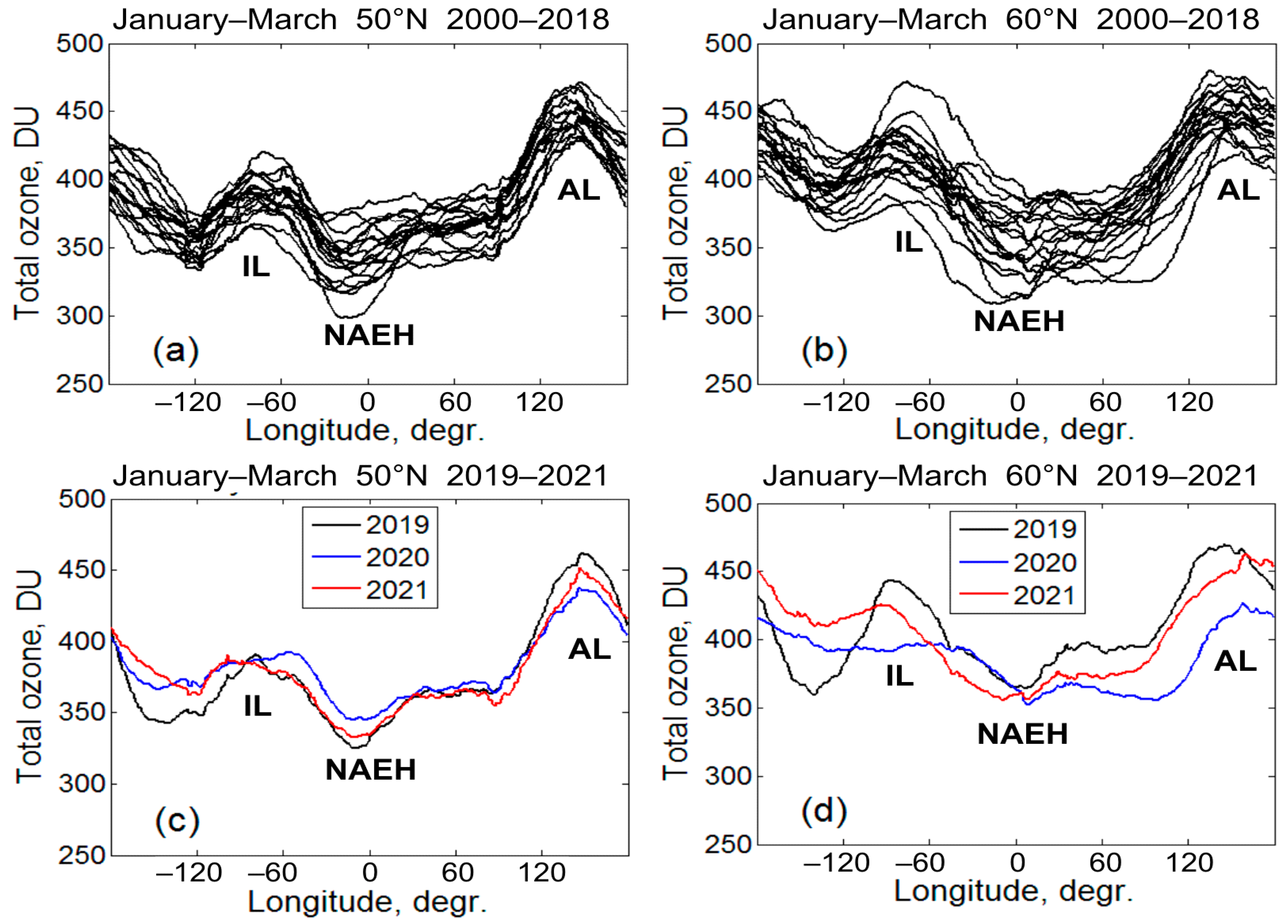
3.1. Total Ozone Zonal Distribution

It should be firstly noted that the TOC zonal distribution in the middle and high latitudes of the northern hemisphere is significantly non-uniform, exhibiting the presence of perturbations with different wave numbers (Figure 1). Mostly, there are two quasi-stationary maxima: over East Asia (longitude about 150°) and North America (longitude about −70°). These maxima are formed due to the action of the two tropospheric centers of action, the Aleutian and Icelandic Lows (AL and IL in Figure 1), where the height of the tropopause is decreased and columnar contribution of stratospheric ozone is increased [11]. These pressure anomalies are responsible for the quasi-stationary wave-2 (QSW2) pattern in the mid- and high-latitude atmosphere. Since the Icelandic Low is a high-latitude center of action near −70° longitude, it provides a higher TOC maximum at 60°N (Figure 1b,d) than at 50°N (Figure 1a,c).
There is an increasing range of TOC variability at 60°N (Figure 1b,d) compared to 50°N (Figure 1a,c), because the westerly zonal flow at the polar vortex edge (~60°N [15]) is more sensitive to the planetary wave influence than the sub-vortex atmosphere. A large difference is observed between 2019 and 2020 at 60°N (black and blue curves in Figure 1d). This is a result of strong and weak low-pressure anomalies in 2019 and 2020, respectively, associated with IL (of about −70° longitude) and AL (~140° longitude). Relatively strong IL and AL pressure anomalies also repeated in 2021 (red curve in Figure 1d). We note the relatively weak longitudinal TOC changes at 60°N in 2020 (blue curve in Figure 1d). This was due to low planetary wave activity in winter, a strong Arctic polar vortex and very low TOC inside the vortex ([7]; see Section 3.3. below). Particularly, the decreased TOC is seen along the eastern longitudes (blue curve in Figure 1d).
The lowest TOC levels near 0° longitude (340–370 Dobson Units, DU) and the highest ones near 140° longitude (around 450 DU) in Figure 1c,d represent the quasi-stationary wave 1 (QSW1) pattern. The zonal TOC minimum is more distinct at 50°N and more extended at 60°N (Figure 1c,d). In both cases, the zonal TOC minimum is associated with a high pressure anomaly—the North Atlantic–European High (NAEH) [23,24].
Next, we consider variations in the amplitudes and phases of the Rossby waves of spectral components with zonal numbers 1–5 at latitude of 60°N, i.e., in the edge region of the polar vortex.

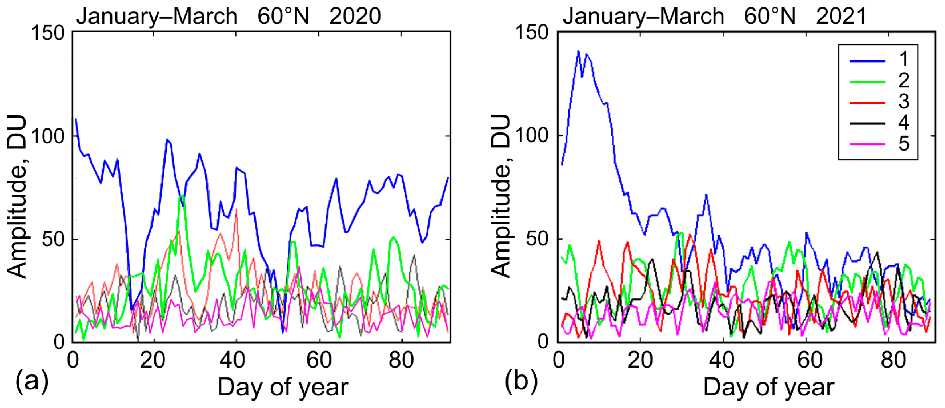
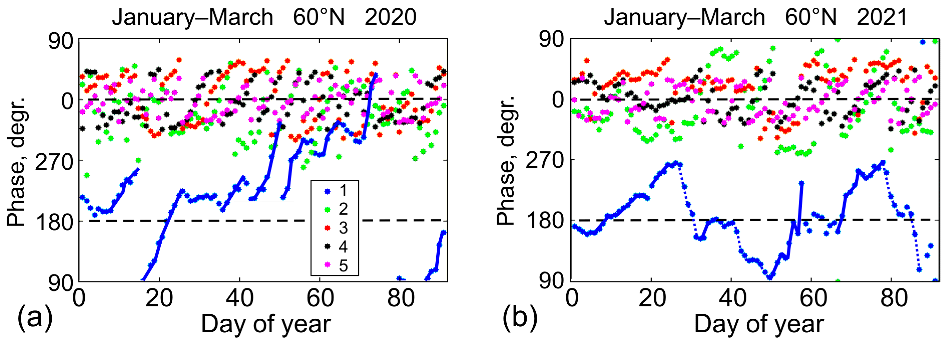
3.2. Daily Variations

Daily variability of wave numbers m = 1–5 in January–March 2020 and 2021 is shown in Figure 2. As noted above, these years represent weak and strong planetary wave activity, resulting in a respectively strong and weak Arctic polar vortex. Wave amplitudes in Figure 2 characterize the combined variability of both quasi-stationary waves (QSWs) and traveling waves at the vortex region (60°N). It is seen that the total wave 1 (blue curve in Figure 2) dominates among the spectral harmonics; however, amplitude variations in 2020 and 2021 differ significantly. The next largest amplitude corresponds to wave 2 (green curves in Figure 2); however, it is a few times lower than the wave-1 amplitude (blue curves). Wave 2 is associated with the Aleutian and Icelandic Lows (Section 3.1).
In 2021, the wave-1 amplitude increased sharply in early January up to 140 DU, dropped in mid-January, and remained below 50 DU in February and March (Figure 2b). Strong wave-1 intensity in early January 2021 caused abrupt weakening of the Arctic vortex and the SSW onset [25,26]. In January–March 2000, the wave-1 activity was held mainly in range 50–100 DU (Figure 2a). Probably, such a level of wave-1 disturbances was insufficient to trigger SSW. This season was characterized by a very strong and cold polar vortex with record-low stratospheric ozone [3,27], and it can be classified as a non-SSW winter [14]. The amplitudes of the remaining spectral components varied predominantly below 50 DU (Figure 2) and do not appear to have had a noticeable effect on the dynamics of the vortex edge region.
Under strong variability of wave amplitudes, it is important to pay attention to variability of wave phases. The longitudinal position of the maximum of the corresponding spectral component was considered as a measure of phase. The difference between 2020 and 2021 should be noted. In 2020, the wave-1 phase migrated in a wide range of longitudes ± 180°, showing regular eastward shift (blue lines in Figure 3a), while in 2021 it oscillated around ~180° longitude within about ±90°, alternating between eastward and westward shifts (solid and dotted blue lines in Figure 3b) and demonstrating a quasi-stationary behavior. This indicates a relation of the wave-1 phase to the difference in the polar vortex strength and the relatively persistent zonal asymmetry of the vortex in 2021.
To reconstruct the phases of the higher spectral harmonics, we chose their maxima closest to the longitude 0°. The estimated phases are concentrated within the longitude range of about ±60° for m = 3–5 (red, black and pink symbols in Figure 3) and ±90° for m = 2 (green symbols).
Wave 1, as a main wave component (blue curves in Figure 2), determines zonal asymmetry in TOC distribution. Hence, by our phase definition, the main zonal TOC maximum (minimum) in 2021 (Figure 3b) oscillated around 180° (0°) longitudes, in general consistency with Figure 1: the highest (lowest) TOC values appeared over the Aleutian Low region (North Atlantic–European High region; see Section 3.1). A closer examination of the phase dispersion of waves with m = 2–5 also reveals regular shifts, but we do not consider that here, leaving them for a separate analysis.

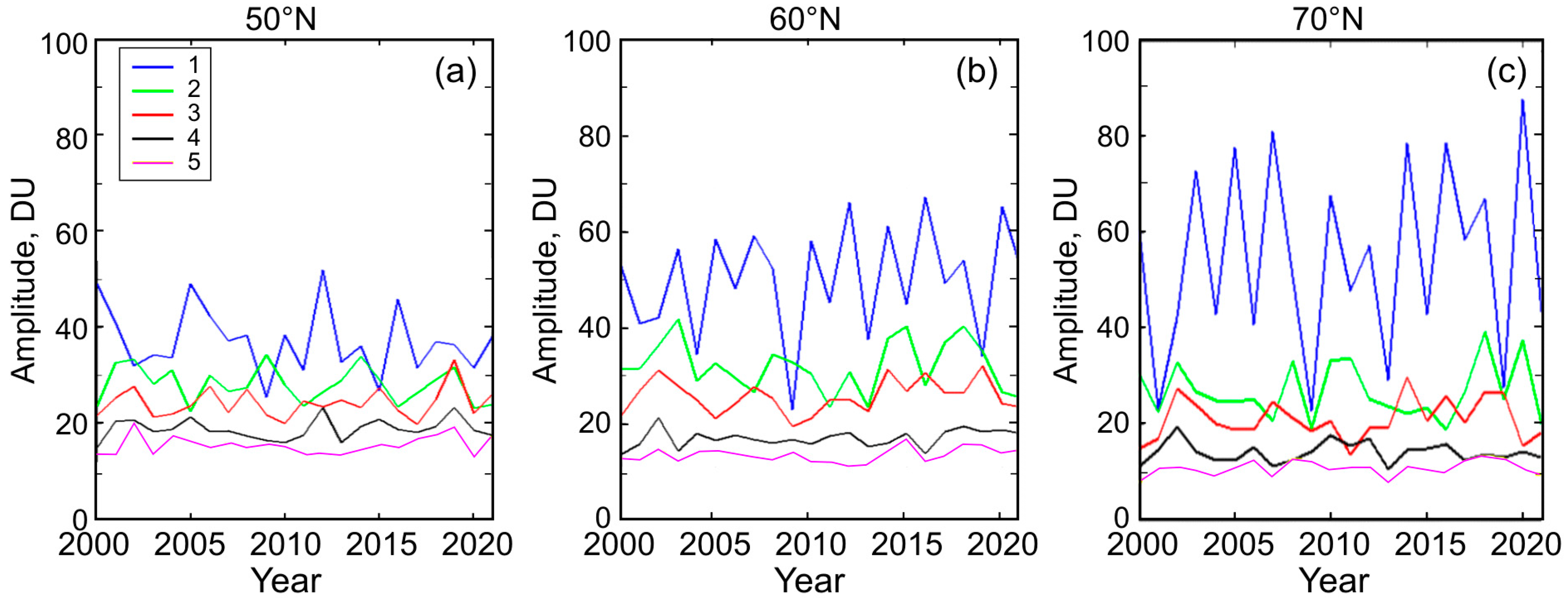
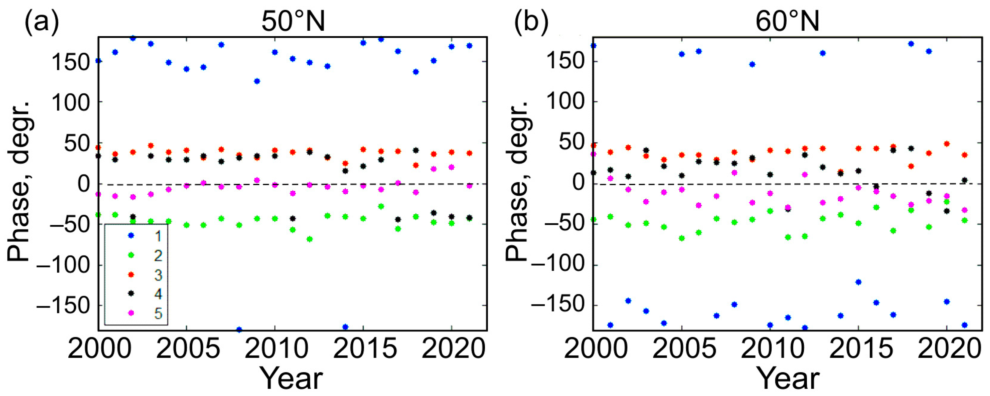
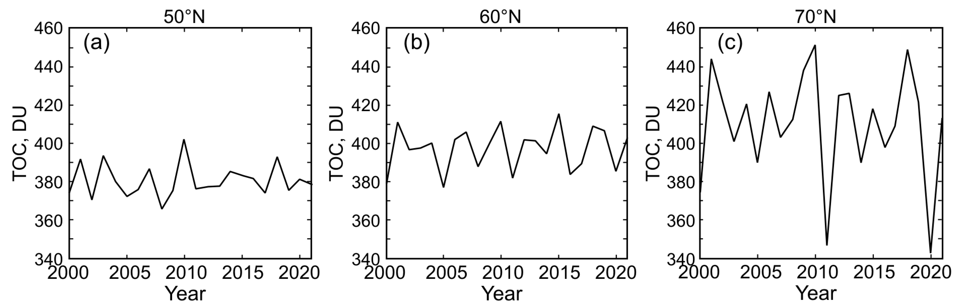
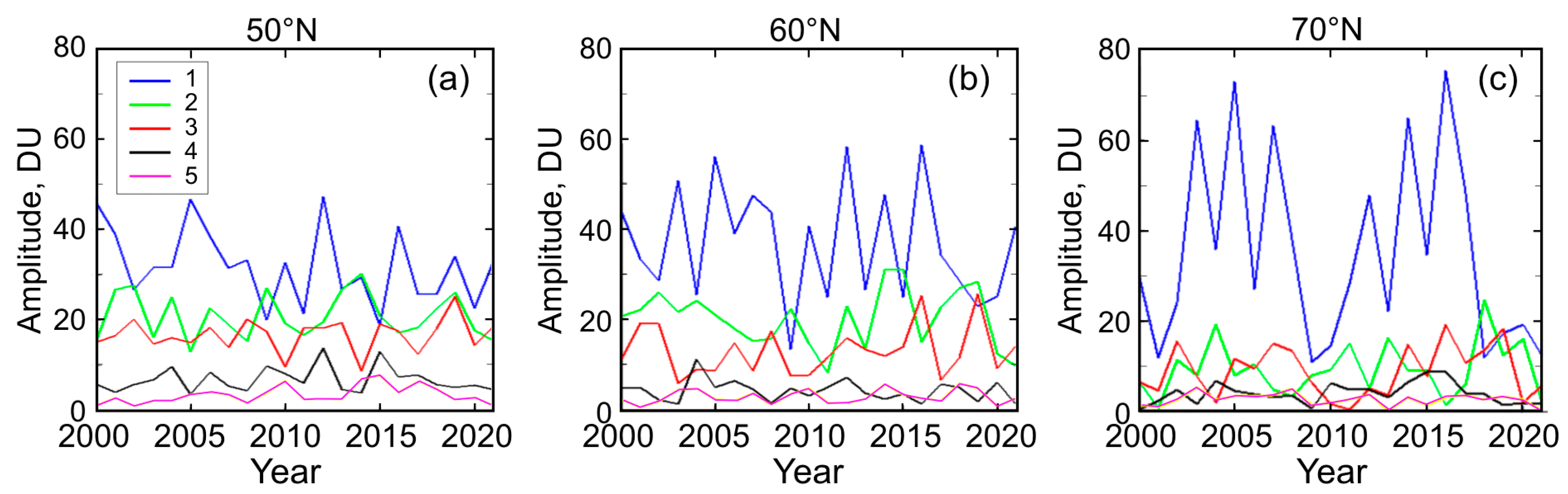
3.3. Interannual Variations
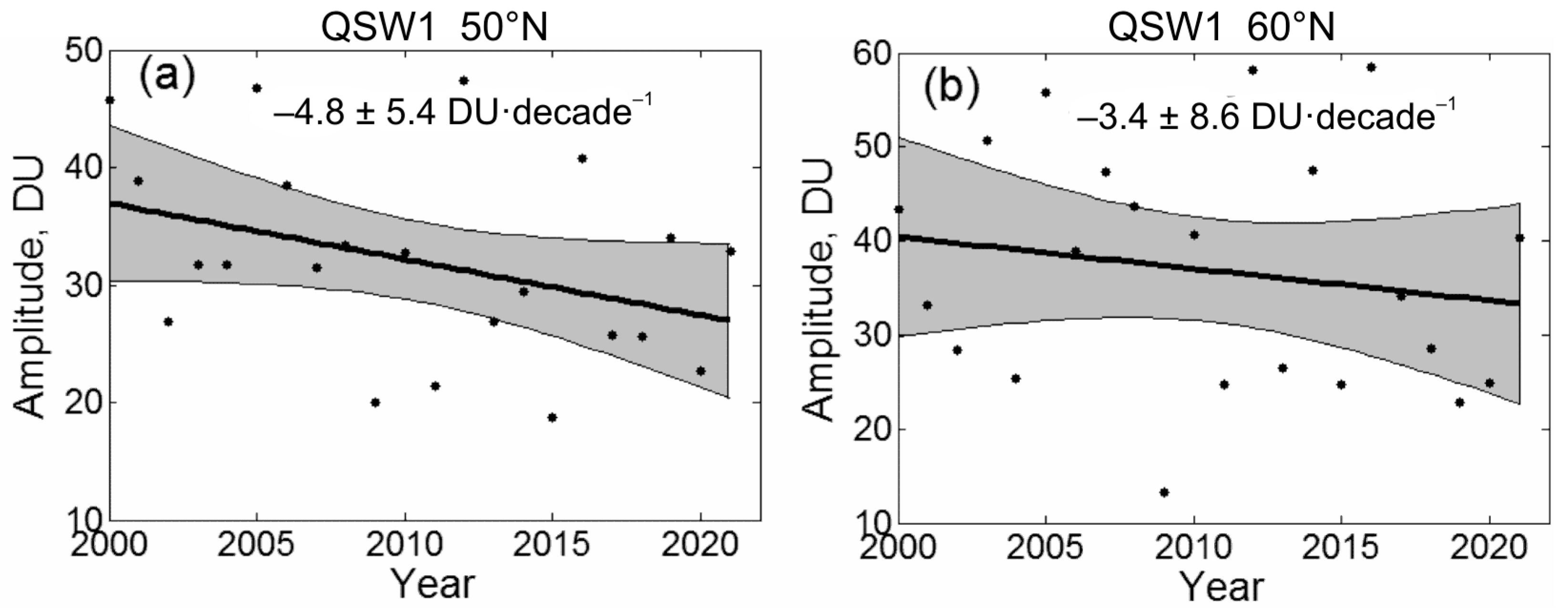
Time series for 2000–2021 in Figure 4a–c show interannual variations of the January–March TOC averages based on zonal means at 50°N, 60°N and 70°N. As noted above, the three selected latitudes represent sub-vortex, vortex-edge and inside-vortex regions, respectively. A positive meridional gradient of TOC with latitude, on an average, from ~380 DU at 50°N to ~400 DU at 60°N and to ~420 DU at 70°N is obvious (Figure 4a–c). This tendency is consistent with poleward ozone transport from the tropics [4,5,12]. Due to Brewer–Dobson circulation, the most intense air descent and the largest stratospheric ozone accumulation occurs in the high-latitude area [5].
It is seen that the positive TOC peaks inside the vortex in 2010 and 2018 alternated with negative ones in 2011 and 2020 (Figure 4c). The latter TOC anomalies correspond to severe depletion of stratospheric ozone over the Arctic in strong vortex conditions due to anomalously low planetary wave activity [7]. No extremely low TOC anomalies were observed in sub-vortex and vortex-edge regions (Figure 4a,b). This confirms the importance of Rossby wave activity in modulating the vortex strength and the resulting chemistry of polar cap ozone causing the appearance of both the anomalously high and low TOC levels.
Among the spectral components with zonal wave numbers 1–5, wave 1 (blue curve in Figure 5) provides the main contribution to the observed interannual variations in TOC (Figure 4). The amplitude of wave 1 increases poleward on an average from ~40 DU (50°N) to ~50 DU (60°N) and ~60 DU (70°N), while the amplitudes of waves 2–5 undergo only small changes between 50°N and 70°N. Wave 2 amplitude remains near the mean level of 30 DU with relatively weak interannual variability (green curve in Figure 5). Note the large range of variations in wave-1 amplitude at 70°N between about 30 DU and 80 DU (Figure 4c).
The TOC anomalies at 70°N noted in wave 1 from Figure 4c are not in strong agreement in time with the wave-1 amplitude anomalies in Figure 5c. This is because the wave amplitude in Figure 5 contains both quasi-stationary waves and traveling waves, and the relation between them can affect TOC changes. It should also be noted that the 3-month averages smooth out sharp peaks that can appear in individual months (Figure 2) and contribute to overall TOC dynamics. Other factors, such as the phases of the Quasi-Biannual Oscillation (QBO) and El Niño—Southern Oscillation (ENSO), can also affect the Arctic vortex strength and TOC variations [15].
The QSW1 amplitude in Figure 6c (blue curve) demonstrates more consistency with TOC (Figure 4c) in variability. The low QSW1 amplitudes in 2011 and 2020 agree in general with the strong vortex conditions. The relationship between the amplitudes of total wave m = 1 and QSW1 at 60°N in 2020 and 2021 also reveals a difference in the vortex strength between these years. Estimation shows, for example, that the QSW1 amplitude consisted 38% of the total wave-1 amplitude in 2020 (25 DU vs. 65 DU) and 73% in 2021 (40 DU versus 55 DU, Figure 5b and Figure 6b). This means that the QSW1 variability is one of the main factors influencing polar vortex strength and polar ozone variability.
The QSW2 amplitudes in January–March 2000–2021 vary around ~20 DU at 50°N and 60°N (green curves in Figure 6a,b) and were comparable with QSW1 (blue curves) in some of the other years shown. However, they decrease to about 10 DU at 70°N, which is, on an average, about 5 times lower than the QSW1 amplitudes (green and blue curves in Figure 6c). It can be seen that the relative role of QSW2 in the interannual TOC variations increases between the vortex (70°N) and sub-vortex (50°N) regions, mainly due to the significant weakening of QSW1.

3.4. Linear Trends

Due to large changes in the zonal TOC distribution from year to year (Figure 1), the zonal wave amplitudes demonstrate a wide range of variability (Figure 7). The relatively short time interval of two decades (2000–2021) makes it difficult to obtain reliable estimates of decadal trends. Figure 7 illustrates linear trends of the QSW1 amplitude at 50°N and 60°N (blue curves in Figure 6a,b). Corresponding to a narrower range of variations in TOC in sub-vortex region (50°N in Figure 4a), the negative trend in Figure 7a of −4.8 DU decade−1 is more reliably at 90% confidence level. Increased TOC variability at the vortex edge region (60°N in Figure 4b) leads to a statistically insignificant trend in the QSW1 amplitude (−3.4 ± 8.6 DU decade−1 in Figure 7b).
No significant trends were identified at 70°N, as well as in the amplitudes of QSW2 or total wave, at all latitudes studied (they are mainly close to zero; not shown). The QSW1 amplitude trend of −4.8 DU per decade at 50°N (Figure 7a) means amplitude decrease by ~10 DU during 21 annual intervals (2000–2021), or by 33% relative to mean level (32 DU). The observed decrease in QSW1 amplitude leads to its approach to the QSW2 amplitude at the end of the study period, since the latter does not undergo significant changes.
Interesting results are obtained when considering the phases of the quasi-stationary components with m = 1–5 (Figure 8). The phase relationship between individual QSW harmonics, averaged over January–March (Figure 8), differs markedly from what is seen from daily variability of the total wave phase (Figure 3).
It turns out that relative phase stability is observed for all zonal wave numbers with an expectedly wider range of variability at 60°N than at 50°N (Figure 8b and Figure 8a, respectively). As the phases indicate the longitudes of the QSW1–QSW3 maxima, they persist at about 180° (QSW1), −40° (QSW2) and 40° (QSW3) longitudes.

4. Discussion

In this paper, we review the main characteristics of the Rossby waves in total ozone in the Arctic region over the past two decades (2000–2021). Qualitatively, the TOC longitudinal structure in January–March (Figure 1) is determined by the atmospheric centers of action in the Northern Hemisphere responsible for the QSW1 and QSW2 patterns [11]. Unlike many previous studies, considering the role of planetary wave driving in the TOC variability and trends [4,8,11,19], we pay attention to the contribution of the amplitudes and phases of the Rossby wave harmonics with zonal numbers m = 1–5 to the TOC variations (Figure 2, Figure 3, Figure 5, Figure 6 and Figure 8). Separately, the interannual variations in the QSW, the total wave (consisting both the quasi-stationary and traveling components) and TOC are compared (Figure 1, Figure 4, Figure 5 and Figure 6).
Theoretically, free and forced Rossby waves exist in the atmosphere [28,29,30]. In our case, with 3-month averaging, the waves forced in the troposphere by the topography and thermal ocean–land contrast and propagating upward into the stratosphere are observed as quasi-stationary in zonal TOC distribution (Figure 1). The QSW structure is sensitive to the east–west location of the forcing regions [28], so the QSW spectral components are characterized by quasi-stationary phases (Figure 8). In the daily variations, the waves freely migrating in the zonal direction can be present (Figure 3). These type of the waves, named “free traveling Rossby wave normal modes”, which are associated with intrinsic atmospheric properties, appear in a perturbed background zonal flow [29].
Three main properties of Rossby waves in the Arctic region are demonstrated by our results. First, the upper threshold of the daily total wave-1 amplitude at 60°N provides some discrimination for identifying winters that show an SSW event and those that do not (i.e., a non-SSW winter as defined by Hu et al. [14]). For example, the cases of 2020 and 2021 show that amplitudes < 100 DU and ~140 DU are associated with winters without SSW and with SSW, respectively (Figure 2a,b). Second, the relative contribution of the QSW1 amplitude to the total wave amplitude appears to reflect the overall dynamics of the vortex. In 2021, QSW1 amounted to 73% of the total wave, which was not only an important factor in SSW occurrence but also led to a quasi-stationary TOC asymmetry around 180° longitude (Figure 3b). This contrasts with 2020, when QSW1 accounted for 38% of the total wave, traveling waves dominated, and there was permanent eastward rotation of the vortex edge (Figure 3a). Third, a stable tendency is an increase in wave amplitudes toward the pole (Figure 5 and Figure 6), which indicates an increase in disturbances in the TOC field (Figure 4), reaching a maximum in the polar cap (Figure 4c).
As noted in Section 3.1, the two quasi-stationary planetary wave troughs in the troposphere, AL and IL, are associated with low tropopause height and, therefore, are anti-correlated with TOC, similar to the situation with synoptic waves [11]. The stratospheric anticyclone above the tropospheric AL is a consequence of westward tilt with altitude of the North American High near −130° longitude in the troposphere [31]. This explains why the total ozone maximum due to the tropopause effect over the Aleutian Low formally coincides with stratospheric anticyclone in this region. Originating in the AL region, the QSW trough shifts westward with altitude into the middle–upper stratosphere approaching 0° longitude [31]. The relative contributions to TOC from middle–upper stratosphere ozone is much lower than from that in the lower stratosphere, where there is a maximum of ozone in the vertical ozone profile. Therefore, above the tropopause trough associated with AL, the contribution to TOC from lower-stratospheric ozone dominates. As found from the Microwave Limb Sounder ozone data, the largest contribution to wave amplitude in TOC comes from ozone layers at 50–100 hPa (not shown).
The North Atlantic–European High (NAEH) is associated with wintertime atmospheric blocking in the North Atlantic–European region [23,24]. The lowest TOC levels (zonal TOC minimum) in Figure 1 are located between −30° and 0° longitudes. This is the region where the NAEH contributes to the rise of the tropopause and the decrease in TOC.
Since TOC is determined mainly by stratospheric ozone, stratospheric ozone loss results in its decrease. In [3,7,26], severe chemical loss in spring 2020 is compared with that in 2011, which is consistent with Figure 1c. In both winters, very strong and cold polar vortices were formed due to less active upward propagation of planetary waves [26]. Low wave activity and cold vortex conditions are accompanied by large PSC volume [7] and low ozone transport into the vortex region [3]. So, under constant seasonal change of sunlight from year to year, low wave activity—low vortex temperature—large PSC volume (exposure of ozone to sunlight under large PSC volume)—low ozone transport become interconnected processes in winter, leading to large stratospheric ozone loss in general agreement with the results of Figure 2a (low wave-1 amplitude in 2020) and Figure 4c (low TOC in the polar vortex region at 70°N in 2020).
We also examined the relationship between an annular mode named the Arctic Oscillation (AO), which is a key factor of climate variability in the Northern Hemisphere [32], and TOC in Figure 4. Using the AO index from the Climate Prediction Center [33], it was found that AO and TOC negatively correlate with correlation coefficients r = −0.40 ± 0.36 and r = −0.56 ± 0.29 (at the 95% confidence level) in middle (50°N) and high (70°N) latitudes, respectively. This indicates a relatively close coupling between AO and TOC in 2000–2021. Quantitatively, AO explains 16% and 31% of TOC variability at 50°N and 70°N, respectively. This is in general consistency with polar vortex strengthening and cooling with increased positive polarity of the AO index, which is accompanied by negative ozone anomalies [32]. The result of Figure 4c, where extremely low TOC in 2011 and 2020 appeared under conditions of a strong and prolonged polar vortex, confirms this interpretation. Particularly high positive AO = 2.7 was in January–March 2020.
The lower TOC variability in the sub-vortex region (Figure 4a) favors a statistically significant negative trend (at the 90% confidence level) in the QSW1 amplitude at 50°N (Figure 7a). At the same time, the interannual TOC variations in Figure 4 are quite significant and, due to the relatively short time series, the trends in TOC are not statistically reliable. This TOC pattern is closely related to the state of the stratospheric polar vortex, its asymmetry relative to the pole and spatial variability [3,34], as well as to variability in meridional ozone transport from the tropics and its accumulation at high latitudes due to Brewer–Dobson circulation [4,5,12].
In Section 3.3, we noted that the interannual variability of polar TOC levels (Figure 4c) is not in strict agreement with the wave amplitudes in Figure 5c and Figure 6c. Other factors, such as the phases of QBO and ENSO, can also affect Arctic vortex strength and TOC variations [15].

5. Conclusions

Based on the TOMS and OMI data sets for January–March 2000–2021, we analyzed the total ozone zonal distribution and variations in the Fourier zonal wave numbers m = 1–5. We considered daily and interannual variations in TOC, amplitudes and phases of spectral wave components, and linear trends of the QSW1 amplitude.
The peculiarities of the Rossby waves in the Arctic region were studied. We determined the upper threshold of the daily total wave-1 amplitude, which indicates the different behavior of wave amplitude in winters with SSW and without SSW. The wave-1 amplitude in TOC is mostly contributed by lower-stratospheric ozone variations in ozone layers at 50 hPa and 100 hPa, near the ozone maximum in vertical ozone profile. The QSW1 amplitude is determined by the strength of quasi-stationary tropospheric pressure anomalies in the regions of the Aleutian Low and the North Atlantic–European High with a zonal maximum and minimum of TOC, respectively. The AL and NAEH contribute to the corresponding decrease and rise of tropopause and the appearance of a zonal TOC maximum and minimum at ~140° longitude and between −30° and 0° longitudes, respectively. The wave amplitudes and disturbances in the TOC field increase toward the pole, reaching the largest magnitudes in the polar cap.
The Arctic Oscillation, as one of the key factors of climate variability in the Northern Hemisphere, negatively correlates with TOC at the 95% confidence level (r = −0.40 ± 0.36 and r = −0.56 ± 0.29 at 50°N and 70°N, respectively. This indicates relatively close coupling between AO and TOC in 2000–2021. Quantitatively, AO explains 16% and 31% of TOC variability at 50°N and 70°N, respectively. This is in general consistency with polar vortex strengthening and cooling with increased positive polarity of the AO index, which is accompanied by negative ozone anomalies [32].
Summing up, it can be concluded that the Rossby wave parameters over the Arctic in the two past decades (2000–2021) confirm dominance of wave 1 and its quasi-stationary component QSW1 in the polar vortex dynamics known from previous studies [11,13,15,18,28]. At the same time, analysis and estimates of the relative role of the spectral components in the zonal TOC distribution help quantitatively describe in more detail the processes that accompany vortex dynamics: (i) quasi-circumpolar migration of the wave-1 phase in 2020 under strong vortex conditions and quasi-stationary vortex asymmetry with the wave-1 phase oscillation around 180° longitude in 2021, when vortex was weakened due to the contribution of high QSW1 activity; (ii) the SSW occurrence with a possible upper threshold of wave-1 amplitude of about 100 DU for the non-SSW winter based on the 2020 event; and (iii) negative decadal trend in the QSW1 amplitude of −4.8 DU decade−1 at 50°N, significant at 90% confidence level.

Author Contributions

Conceptualization, A.G., O.E. and G.M.; methodology, A.G. and O.E.; data acquisition, A.G., C.Z. and O.E.; software, Y.A., C.Z. and O.E.; validation, O.E., Y.R., A.K. and G.M.; investigation, O.E., G.M., A.G., A.K., W.H., Y.A. and C.Z.; writing—original draft preparation, A.G., O.E., A.K. and G.M.; writing—review and editing, O.E., A.K., C.Z., Y.R., G.M., Y.A. and V.S.; visualization, A.G., Y.A., O.E. and C.Z.; supervision, G.M.; project administration, G.M., V.S. and W.H. Each author contributed to the interpretation and discussion of the results and edited the manuscript. All authors have read and agreed to the published version of the manuscript.

Funding

This research received no external funding.

Informed Consent Statement

Not applicable.

Acknowledgments

This work was partially supported by the College of Physics, International Center of Future Science, Jilin University, China, and by the Ministry of Education and Science of Ukraine with the grant BN-06 for prospective development of a scientific direction “Mathematical sciences and natural sciences” and the project 20BF051-02 at the Taras Shevchenko National University of Kyiv. This work contributed to Project 4293 of the Australian Antarctic Program, and to the National Antarctic Scientific Center of Ukraine research objectives. We acknowledge the Goddard Earth Sciences Data and Information Services Center for TOC data from Total Ozone Mapping Spectrometer (Earth Probe) and the National Aeronautics and Space Administration, Goddard Space Flight Center for Ozone Monitoring Instrument (Aura) measurements (https://disc.gsfc.nasa.gov/datasets/ and https://ozonewatch.gsfc.nasa.gov/, both accessed on 21 February 2022). We also thank the Climate Prediction Center, NOAA National Weather Service, for Arctic Oscillation index data (https://www.cpc.ncep.noaa.gov/, accessed on 25 April 2022).

Conflicts of Interest

The authors declare no conflict of interest.

References

  1. Matsuno, T. Vertical propagation of stationary planetary waves in the winter Northern Hemisphere. J. Atmos. Sci. 1970, 27, 871–883. [Google Scholar] [CrossRef] [Green Version]
  2. Domeisen, D.I.V.; Butler, A.H. Stratospheric drivers of extreme events at the Earth’s surface. Commun. Earth Environ. 2020, 1, 59. [Google Scholar] [CrossRef]
  3. Manney, G.L.; Livesey, N.J.; Santee, M.L.; Froidevaux, L.; Lambert, A.; Lawrence, Z.D.; Millán, L.F.; Neu, J.L.; Read, W.G.; Michael, J.; et al. Record-low Arctic stratospheric ozone in 2020: MLS observations of chemical processes and comparisons with previous extreme winters. Geophys. Res. Lett. 2020, 47, e2020GL089063. [Google Scholar] [CrossRef]
  4. Weber, M.; Dikty, S.; Burrows, J.P.; Garny, H.; Dameris, M.; Kubin, A.; Abalichin, J.; Langematz, U. The Brewer-Dobson circulation and total ozone from seasonal to decadal time scales. Atmos. Chem. Phys. 2011, 11, 11221–11235. [Google Scholar] [CrossRef] [Green Version]
  5. Butchart, N. The Brewer-Dobson circulation. Rev. Geophys. 2014, 52, 157–184. [Google Scholar] [CrossRef]
  6. Solomon, S.; Garcia, R.; Rowland, F.; Wuebbles, D. On the depletion of Antarctic ozone. Nature 1986, 321, 755–758. [Google Scholar] [CrossRef] [Green Version]
  7. Wohltmann, I.; von der Gathen, P.; Lehmann, R.; Maturilli, M.; Deckelmann, H.; Manney, G.L.; Davies, J.; Tarasick, D.; Jepsen, N.; Kivi, R.; et al. Near-complete local reduction of Arctic stratospheric ozone by severe chemical loss in spring 2020. Geophys. Res. Lett. 2020, 47, e2020GL089547. [Google Scholar] [CrossRef]
  8. Fusco, A.C.; Salby, M.L. Interannual variations of total ozone and their relationship to variations of planetary wave activity. J. Clim. 1999, 12, 1619–1629. [Google Scholar] [CrossRef]
  9. Charney, J.G.; Drazin, P.G. Propagation of planetary-scale disturbances from the lower into the upper atmosphere. J. Geophys. Res. 1961, 66, 83–109. [Google Scholar] [CrossRef]
  10. Domeisen, D.I.V.; Martius, O.; Jiménez-Esteve, B. Rossby wave propagation into the Northern Hemisphere stratosphere: The role of zonal phase speed. Geophys. Res. Lett. 2018, 45, 2064–2071. [Google Scholar] [CrossRef] [Green Version]
  11. Hood, L.L.; Zaff, D.A. Lower stratospheric stationary waves and the longitude dependence of ozone trends in winter. J. Geophys. Res. 1995, 100, 25791–25800. [Google Scholar] [CrossRef]
  12. Dütsch, H.U. The ozone distribution in the atmosphere. Can. J. Chem. 1974, 52, 1491–1504. [Google Scholar] [CrossRef]
  13. Alexander, S.P.; Shepherd, M.G. Planetary wave activity in the polar lower stratosphere. Atmos. Chem. Phys. 2010, 10, 707–718. [Google Scholar] [CrossRef] [Green Version]
  14. Hu, J.; Ren, R.; Xu, H. Occurrence of winter stratospheric sudden warming events and the seasonal timing of spring stratospheric final warming. J. Atmos. Sci. 2014, 71, 2319–2334. [Google Scholar] [CrossRef]
  15. Baldwin, M.P.; Ayarzagüena, B.; Birner, T.; Butchart, N.; Butler, A.H.; Charlton-Perez, A.J.; Domeisen, D.I.V.; Garfinkel, C.I.; Garny, H.; Gerber, E.P.; et al. Sudden stratospheric warmings. Rev. Geophys. 2021, 59, e2020RG000708. [Google Scholar] [CrossRef]
  16. Butler, A.H.; Sjoberg, J.P.; Seidel, D.J.; Rosenlof, K.H. A sudden stratospheric warming compendium. Earth Syst. Sci. Data 2017, 9, 63–76. [Google Scholar] [CrossRef] [Green Version]
  17. Butler, A.H.; Gerber, E.P. Optimizing the definition of a Sudden Stratospheric Warming. J. Clim. 2018, 31, 2337–2344. [Google Scholar] [CrossRef]
  18. Butler, A.H.; Domeisen, D.I.V. The wave geometry of final stratospheric warming events. Weather Clim. Dyn. 2021, 2, 453–474. [Google Scholar] [CrossRef]
  19. Dhomse, S.; Weber, M.; Wohltmann, I.; Rex, M.; Burrows, J.P. On the possible causes of recent increases in northern hemispheric total ozone from a statistical analysis of satellite data from 1979 to 2003. Atmos. Chem. Phys. 2006, 6, 1165–1180. [Google Scholar] [CrossRef] [Green Version]
  20. Levelt, P.F.; Joiner, J.; Tamminen, J.; Veefkind, J.P.; Bhartia, P.K.; Zweers, D.C.S.; Duncan, B.N.; Streets, D.G.; Eskes, H.; van der A, R.; et al. The Ozone Monitoring Instrument: Overview of 14 years in space. Atmos. Chem. Phys. 2018, 18, 5699–5745. [Google Scholar] [CrossRef] [Green Version]
  21. OMI: NASA Ozone Watch, National Aeronautics and Space Administration, Goddard Space Flight Center, Ozone Monitoring Instrument. Available online: https://ozonewatch.gsfc.nasa.gov/ (accessed on 21 February 2022).
  22. TOMS: Total Ozone Mapping Spectrometer, Goddard Earth Sciences Data and Information Services Center (GES DISC). Available online: https://disc.gsfc.nasa.gov/datasets/ (accessed on 21 February 2022).
  23. Bacer, S.; Jomaa, F.; Beaumet, J.; Gallée, H.; Le Bouëdec, E.; Ménégoz, M.; Staquet, C. Impact of climate change on wintertime European atmospheric blocking. Weather Clim. Dyn. 2022, 3, 377–389. [Google Scholar] [CrossRef]
  24. Haarsma, R.J.; García-Serrano, J.; Prodhomme, C.; Bellprat, O.; Davini, P.; Drijfhout, S. Sensitivity of winter North Atlantic-European climate to resolved atmosphere and ocean dynamics. Sci. Rep. 2019, 9, 13358. [Google Scholar] [CrossRef] [PubMed] [Green Version]
  25. Hongming, Y.; Yuan, Y.; Guirong, T.; Yucheng, Z. Possible impact of sudden stratospheric warming on the intraseasonal reversal of the temperature over East Asia in winter 2020/21. Atmos. Res. 2022, 268, 106016. [Google Scholar] [CrossRef]
  26. Lu, Q.; Rao, J.; Liang, Z.; Guo, D.; Luo, J.; Liu, S.; Wang, C.; Wang, T. The sudden stratospheric warming in January 2021. Environ. Res. Lett. 2021, 16, 084029. [Google Scholar] [CrossRef]
  27. Zhang, Y.; Cai, Z.; Liu, Y. The exceptionally strong and persistent Arctic stratospheric polar vortex in the winter of 2019–2020. Atmos. Ocean. Sci. Lett. 2021, 14, 100035. [Google Scholar] [CrossRef]
  28. Rhines, P.B. Rossby waves. In Encyclopedia of Atmospheric Sciences; Holton, J.R., Ed.; Academic Press: Cambridge, MA, USA, 2003; pp. 1923–1939. [Google Scholar] [CrossRef]
  29. Madden, R.A. Large-scale, free Rossby waves in the atmosphere—An update. Tellus A Dyn. Meteorol. Oceanogr. 2007, 59, 571–590. [Google Scholar] [CrossRef]
  30. Sassi, F.; Garcia, R.R.; Hoppel, K.W. Large-scale Rossby normal modes during some recent Northern Hemisphere winters. J. Atmos. Sci. 2012, 69, 820–839. [Google Scholar] [CrossRef]
  31. Harvey, V.L.; Hitchman, M.H. A climatology of the Aleutian High. J. Atmos. Sci. 1996, 53, 2088–2102. [Google Scholar] [CrossRef] [Green Version]
  32. Thompson, D.W.J.; Wallace, J.M. Annular modes in the extratropical circulation. Part I: Month-to-month variability. J. Clim. 2000, 13, 1000–1016. [Google Scholar] [CrossRef]
  33. AO: Arctic Oscillation Index, NOAA National Weather Service, Climate Prediction Center. Available online: https://www.cpc.ncep.noaa.gov/ (accessed on 25 April 2022).
  34. McCormack, J.P.; Nathan, T.R.; Cordero, E.C. The effect of zonally asymmetric ozone heating on the Northern Hemisphere winter polar stratosphere. Geophys. Res. Lett. 2011, 38, L03802. [Google Scholar] [CrossRef] [Green Version]
Figure 1. Zonal distributions of TOC along latitudes (a,c) 50°N and (b,d) 60°N averaged for January–March and their interannual variations in (a,b) 2000–2018 and (c,d) 2019, 2020 and 2021. Longitude 0° corresponds to Greenwich meridian, positive longitudes are east of the 0° meridian. AL is Aleutian Low, IL is Icelandic Low and NAEH is North Atlantic–European High.
Remotesensing 14 02192 g001
Figure 2. Daily variations in the amplitudes of the Fourier spectral components with zonal wave numbers m = 1–5 at the latitude 60°N in January–March (a) 2020 and (b) 2021.
Remotesensing 14 02192 g002
Figure 3. Daily variations in phases of the Fourier spectral components with zonal wave numbers m = 1–5 at a latitude 60°N in January–March (a) 2020 and (b) 2021.
Remotesensing 14 02192 g003
Figure 4. Interannual variations in zonal mean TOC values in 2000–2021, averaged over January–March. The latitudes (a) 50°N, (b) 60°N and (c) 70°N are presented.
Remotesensing 14 02192 g004
Figure 5. Interannual variations of amplitudes of spectral wave components with m = 1–5 in 2000–2021, averaged over January–March. The latitudes (a) 50°N, (b) 60°N and (c) 70°N are presented.
Remotesensing 14 02192 g005
Figure 6. Interannual variations of amplitudes of quasi-stationary wave components with m = 1–5 (QSW1–QSW5) in 2000–2021, averaged over January–March. The latitudes (a) 50°N, (b) 60°N and (c) 70°N are shown.
Remotesensing 14 02192 g006
Figure 7. Interannual variations and linear trends of amplitudes of quasi-stationary spectral component with zonal wave number m = 1 (QSW1) in 2000–2021, averaged for January–March, at (a) 50°N and (b) 60°N. The confidence interval of the trend at the significance level of 95% is shaded.
Remotesensing 14 02192 g007
Figure 8. Interannual variations of phases of quasi-stationary spectral components with zonal wave numbers m = 1–5 in 2000–2021, averaged over January–March, at (a) 50°N and (b) 60°N.
Remotesensing 14 02192 g008
Publisher’s Note: MDPI stays neutral with regard to jurisdictional claims in published maps and institutional affiliations.

