Abstract
An understanding of land and sea surface backscatter coefficients at high frequencies (HF) is required to accurately assess ionospheric propagation conditions for over-the-horizon radar. In this paper, two methods of calculating sea surface backscatter coefficients are compared. The first method is a theoretical method developed by Barrick in 1972, which treats the sea as a slightly rough surface defined by a wave height spectrum and uses a perturbation approach. The second method compares the difference between observed and modelled backscatter ionograms in which all other losses are accounted for to obtain a measurement of the sea surface backscatter coefficient. Similar trends and values for the sea surface backscatter coefficients from each method were found despite the many models and assumptions required for both these methods. However, it was noted that there was a larger range of values for the sea surface backscatter coefficients when the Barrick method was used.
1. Introduction
The backscatter coefficient of the sea for radio waves in the high-frequency (HF) band has been well researched over many years, as there has been a strong interest for applications such as the detection of near surface military targets and for remote sensing of the sea state [1,2]. For over-the-horizon radar, an understanding of surface backscatter coefficients is important for assessing the ionospheric propagation conditions. The sea surface backscatter coefficient characterizes the amount of radiation that is scattered back from the sea surface towards a receiver per unit area. It is dependent on the depth of the water, the wind speed, the wave heights and the ocean surface currents [3]. Our earlier paper [4] describes a method of calculating the surface backscatter coefficients using backscatter ionograms [5].
From ground wave measurements at HF, the backscatter coefficient of a fully developed sea (where the waves have reached an equilibrium with the wind) is approximately −23 dB [6]. Radio waves scattered back from the sea also have a characteristic Doppler shift caused by the coherent Bragg scattering of the signal from components of the sea wave height spectrum that are moving towards or away from the radar with wavelengths half the radio wavelength [2,7].
The sea surface backscatter coefficient can be theoretically modelled by treating the sea surface as a slightly rough surface and then using a perturbation method to calculate the reflection of electromagnetic waves [8,9]. The sea surface can be described using a directional wave height spectrum, which describes the distribution of wave energy as a function of the wave frequency. Equations for the sea surface backscatter coefficient from a directional wave height spectrum in deep and shallow water were derived by Barrick using the boundary perturbation approach [3,9]. The directional wave height spectrum was assumed to be separable into the wave number component and the directional factor by several researchers [10,11]. This theoretical model of the backscatter coefficient is dependent on the wave height spectrum that is used. The Pierson–Moskowitz spectrum is one of the simplest spectra; it is a non-directional spectrum that describes a fully developed sea. The Joint North Sea Wave Observation Project (JONSWAP) spectrum is based on the Pierson–Moskowitz spectrum, with an extra factor included to adjust for a non-fully developed sea [12]. These two sea spectra were used by [13] along with a wave direction factor, and high-resolution wind speed, swell height and swell period data to model sea surface backscatter coefficients.
In this paper, we calculate sea surface backscatter coefficients using the method described by [13] (based on the theory developed by Barrick) with a wave height spectrum obtained from sea state data. We also calculate sea surface backscatter coefficients using a method of comparing observed and modelled backscatter ionograms as described in our earlier paper [4]. The current paper presents a comparison of these two methods of calculating sea surface backscatter coefficients at HF. Section 2 describes the data used, the two methods used to calculate sea surface backscatter coefficients and an overview of how the methods were compared. Section 3 presents the sea surface backscatter coefficients and a comparison of the results from each method of calculation. The conclusions and future work are described in Section 4.
2. Materials and Methods
2.1. Sea Hindcast Data
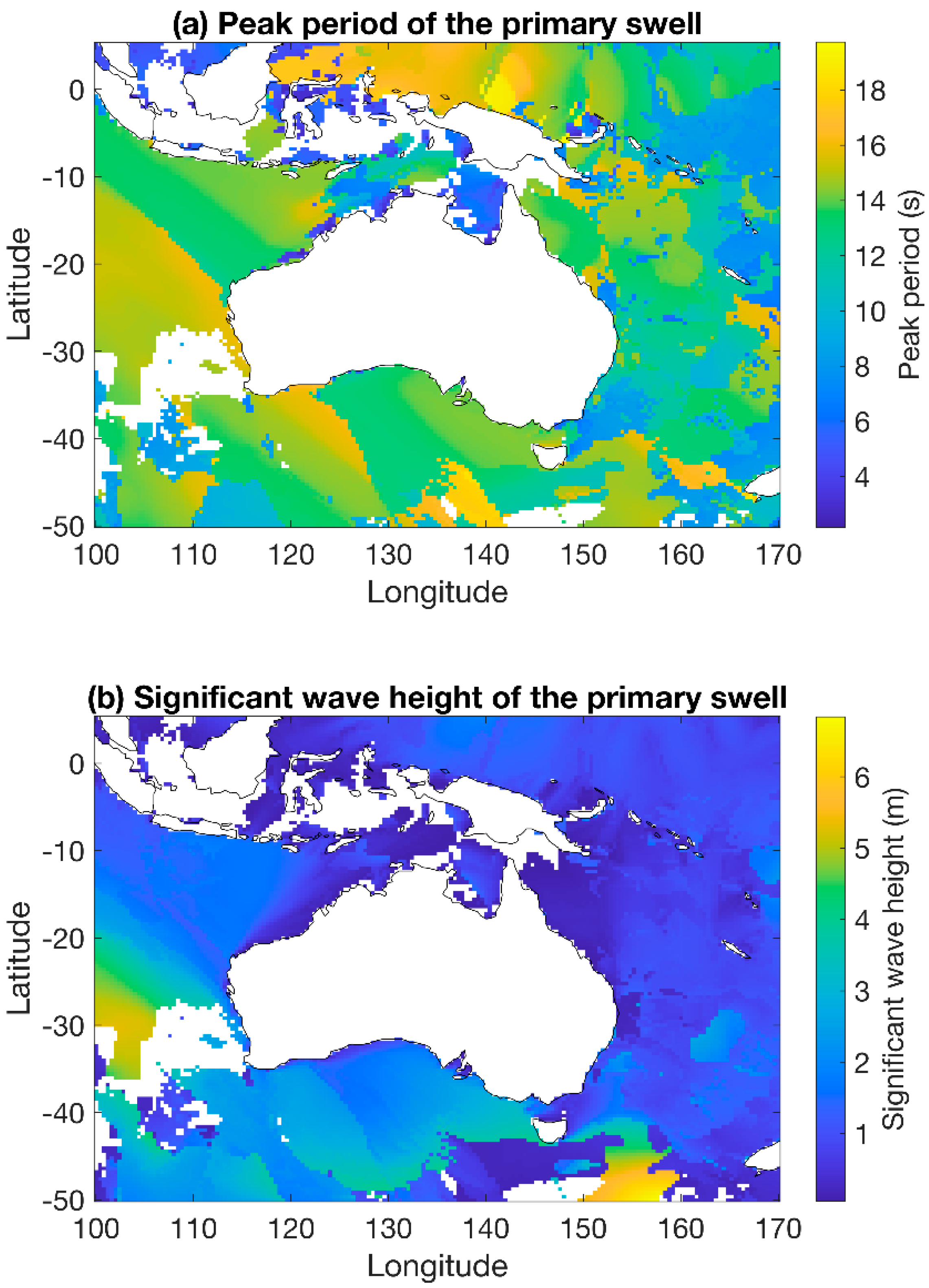
Sea hindcast data for September 2015 and March 2016 were accessed from the Centre for Australian Weather and Climate Research [14]. The hindcast data were produced using the WAVEWATCH III model forced by reanalysed winds [14]. They were available hourly over the globe at 0.4° resolution and available at a resolution of 10 arcminutes over the South Pacific and the Australian coast. Many parameters were available from this data set; but for this work, only the significant wave height (m) and peak period (s) of the primary, secondary and tertiary swells and the wind sea were used along with the northward and eastward components of the wind (m/s). Primary, secondary, and tertiary swells are generated by distant weather systems, while wind sea waves are generated by local winds. Figure 1 shows an example of the peak period and the significant wave height of the primary swell from the 0.4° resolution dataset.

Figure 1.
(a) The peak period and (b) the significant wave height of the primary swell using the 0.4° resolution sea hindcast data at 04:00 UT on the 10 September 2015. Data were not available at this time for areas shown in white.
2.2. Calculating Sea Surface Backscatter Coefficients Using the Barrick Method
The backscatter coefficient equations developed by Barrick [9] were used to calculate sea surface backscatter coefficients with the JONSWAP wave height spectrum [12]. The JONSWAP spectrum was calculated using sea state data accessed from the Centre for Australian Weather and Climate Research [14]. This method assumes the wave heights are small compared to the radio wavelength, the surface slopes are small, and the impedance of the surface is small in terms of the free-space wave impedance; these conditions are satisfied by the sea at HF. It is also assumed that the radio waves are at grazing angles, where the angle of incidence is greater than 80 degrees [15].
The sea surface backscatter coefficients were calculated hourly during the day (from 00:00 UT to 10:00 UT) throughout September 2015 and March 2016. These restricted times were used as backscatter coefficients from the backscatter ionogram method (described in Section 2.3) and were only calculated during the daytime. This was due to the greater range of frequencies available for ionospheric propagation [4] during the daytime.
2.2.1. Sea Surface Backscatter Coefficient Equations
Barrick showed that for deep water in the absence of a surface current, the first-order backscatter coefficient can be calculated using the perturbation approximation as the heights of the ocean waves are small compared to the radar wavelength [9,16]. The equation for the first-order backscatter coefficient, dependent on the frequency of the radio wave, is given by
where denotes the sign of the doppler shift, is the magnitude of the incoming radio wavenumber, is the radar wave vector (of magnitude ) in the direction from the radar to the sea surface, is the directional wave height spectrum, and is the ocean wave frequency (Bragg line frequency) associated with [3,17]. The wavelength of the scattering ocean waves is half the radar wavelength, such that the scattering ocean wavenumber is equal to [16]. For deep water, , hence , where is the gravitational acceleration [3].
Using the separable form of the wave height spectrum and the averaged radar cross section of the sea
As the power from both the Bragg lines must be included, Gardiner-Garden and Pincombe [17] and Neller [13] showed that the backscatter coefficient could be given by
where is the wavenumber of the Bragg lines and is the directionality factor. The directionality factor is given by
where is the local angle of the wind (principal wave direction) and is the local angle of the radar beam (i.e., is given by the sum of the radar angle and the wind direction).
The backscatter coefficient is defined as:
where
For the non-directional wave height spectrum, , the JONSWAP spectrum [12] was used.
In the sea state data accessed from the Centre for Australian Weather and Climate Research, there were values for the significant wave height () and the peak period () of the wind waves along with the primary, secondary and tertiary swells. Thus, the backscatter coefficient was calculated by finding the wave height spectrum and backscatter coefficient for each of these swells and then summing the results [13]
The JONSWAP spectrum defines a wind-wave spectrum, and there may be some question as to the use of this spectrum to define the swell spectrum. However, the contribution to the backscatter coefficients from the swell is typically small. That is, the sea surface backscatter coefficient at HF primarily consists of the wind wave component. Only the first-order Bragg scatter is considered in this calculation of the sea surface backscatter coefficient, higher-order backscatter is ignored.
2.2.2. JONSWAP Spectrum
The JONSWAP spectrum is a non-directional wave height spectrum, based on the Pierson–Moskowitz spectrum for a fully developed sea [12]. An extra peakedness factor (calculated empirically) is included to adjust for a non-fully developed sea. The JONSWAP spectrum [12,18] is given by the equation
where
Here, is a normalisation constant, is the gravitational acceleration, is the wave angular frequency (rad/s), is the wave angular peak frequency (rad/s) and is the JONSWAP peakedness parameter. The normalisation constant is defined as
The peakedness parameter is given by
where is the peak period (s) of the wind swell and is the significant wave height (m). The peakedness parameter is limited to from qualitative considerations of deep water wave data from the North Sea [18]. When , the JONSWAP spectrum reduces to the Pierson–Moskowitz spectrum of a fully developed sea. The JONSWAP spectrum can be written in terms of the wave number [13].
The directionality of the wind is included in the manner described above. Hence, the backscatter coefficient when using the JONSWAP spectrum is given by
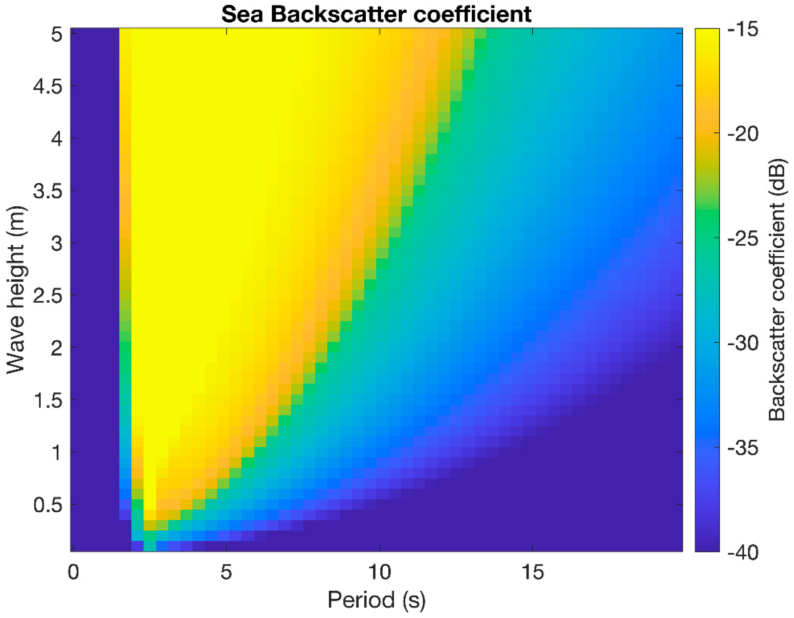
An example of backscatter coefficients calculated using this method is shown in Figure 2.

Figure 2.
The backscatter coefficient calculated for a range of wave heights and periods using the Barrick method for a radar operating at 15 MHz. The radar beam steer angle and wind were in the same direction. Values much greater than that of a fully developed sea (approximately −23 dB) are due to a non-physical combination of wave height and wave period.
2.3. Calculating Backscatter Coefficients Using the Backscatter Ionogram Method
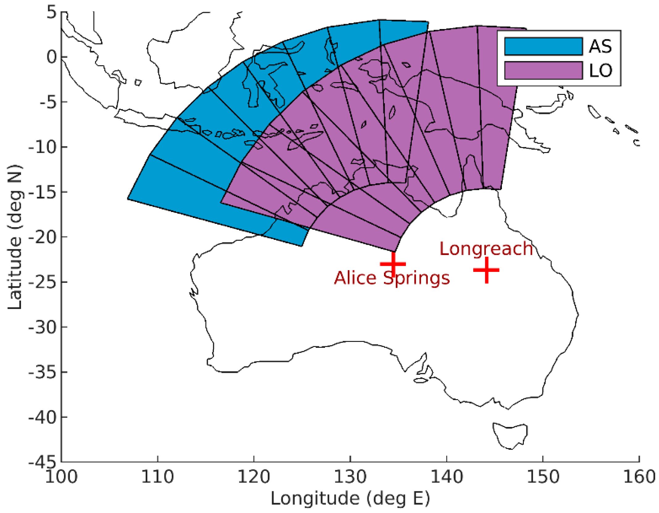
Sea surface backscatter coefficients were also calculated using a method of comparing observed and modelled backscatter ionograms (described in detail in our earlier paper [4]). Backscatter ionograms observed by two Australian backscatter sounders from the JORN frequency management system were used. These sounders were located at Longreach (LO), and Alice Springs (AS). Data collected in September 2015 [19] and March 2016 with a temporal resolution of 5 min were analysed. The group range resolution of this data was 50 km, the frequency resolution was 0.2 MHz, and the power resolution was 0.5 dBW. The ionograms were scaled to a transmit power of 20 kW. Each sounder simultaneously forms eight beams to create eight backscatter ionograms, where the beams are labelled one through to eight from west to north. The location and fields of view of the two backscatter sounders are shown in Figure 3. For a more detailed description of the sounder system and data refer to [4].
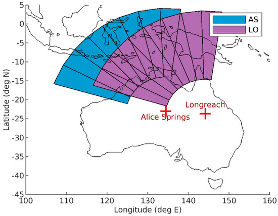
Figure 3.
Backscatter sounder locations, fields of view and disposition of the eight receive beams. The inner and outer arcs are 1000 and 3000 km from the sounders, respectively.
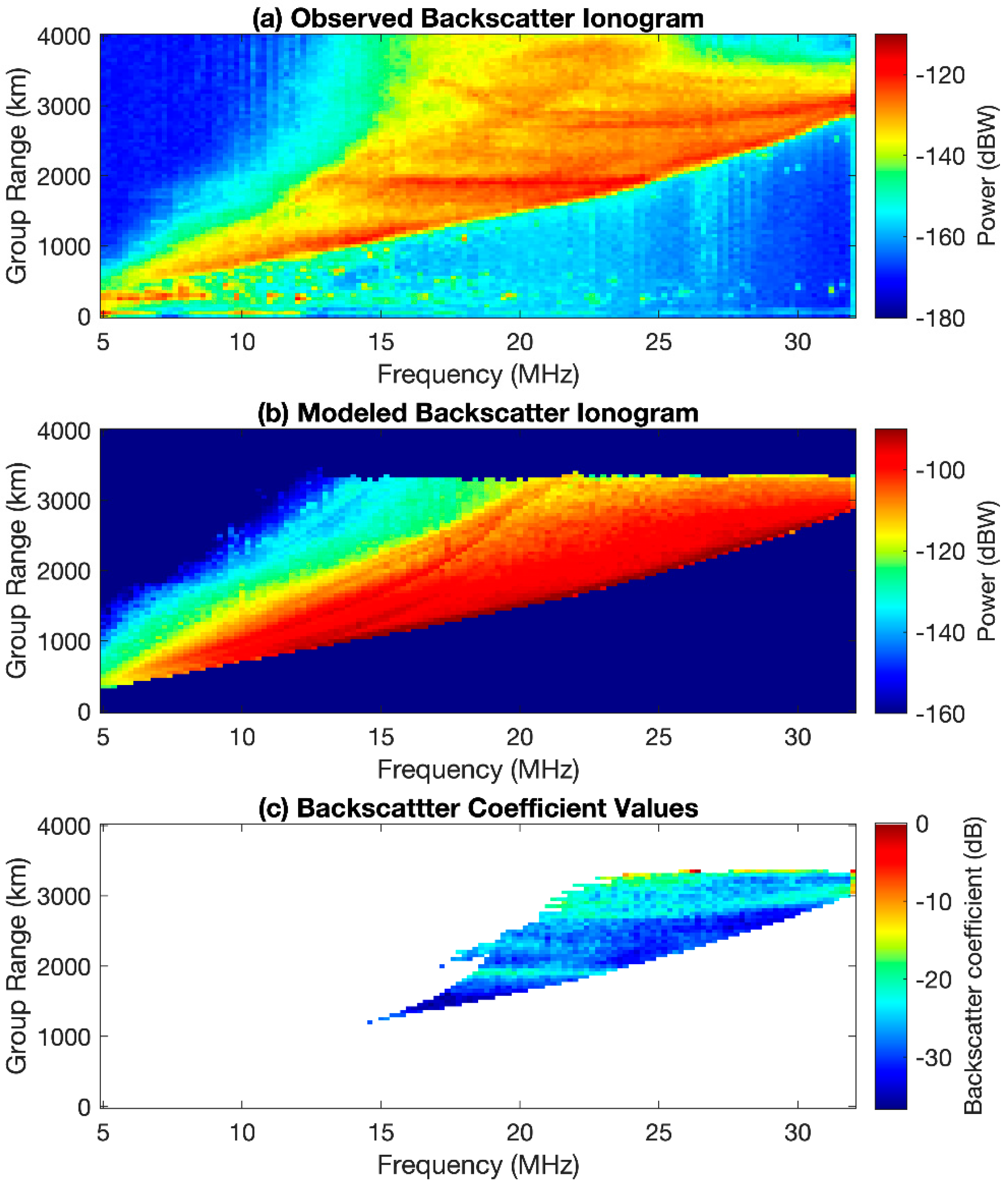
The backscatter coefficient was calculated by taking the difference in power between the observed and modelled ionograms where the backscatter coefficient was set to 0 dB and all other losses were accounted for. Figure 4 shows an example of an observed backscatter ionogram (top panel), a modelled backscatter ionogram from the same time (middle panel) and the backscatter coefficients calculated from the difference between these ionograms (bottom panel). The numerical ray tracing toolbox PHaRLAP [20] was used together with a near real time data-driven model of the ionosphere [21] to model the backscatter ionograms. Propagation losses such as focussing/defocussing and ionospheric absorption were accounted for appropriately, although we note that while the model of the ionosphere was near real time, the climatological ionospheric absorption model of George and Bradley [22,23] was used. The transmit and receive antenna gains were modelled using a method-of-moments electromagnetic solver [24].

Figure 4.
(a) A backscatter ionogram observed by Longreach Beam 2 at 0200 UT on the 3 September 2015. (b) A backscatter ionogram synthesized using models of the environmental conditions at the same time and location as the observed ionogram. (c) Backscatter coefficient values obtained by taking the difference in power between the observed and modelled ionograms.
Backscatter ionograms modelled from 00:00 UT to 10:00 UT (approximately 09:30 to 19:30 local time) for days when observed data were available in September 2015 and March 2016 were used to generate the backscatter coefficient data. These daytime hours were used as more frequencies are available for ionospheric propagation during the day. The median backscatter coefficient was then calculated for each 50 km range cell for each of the 8 receive beams of the sounders to create maps of the backscatter coefficient (as will be shown in Section 3).
2.4. Comparison of the Barrick and Backscatter Ionogram Methods
The backscatter coefficient results from the backscatter ionogram and Barrick methods were compared to investigate the similarities and differences between these methods. The sea surface backscatter coefficients were calculated using the Barrick method with a wave height spectrum calculated from the 10-arcminute sea state hindcast data for a selection of radar frequencies (6–26 MHz in 2 MHz steps) hourly from 00:00 UT to 10:00 UT for September 2015 and March 2016. These frequencies were representative of the typical range of frequencies that the backscatter sounder data yielded reliable backscatter coefficients.
The backscatter coefficient results from the two methods were compared twice per day throughout the months of interest during a morning and afternoon period. The temporal median of the backscatter coefficients from each method was calculated in the morning using results from 00:00 UT to 06:00 UT (approximately 09:30 to 15:30 local time) and in the afternoon using results from 04:00 UT to 10:00 UT (approximately 13:30 to 19:30 local time). These large overlapping time periods were used to increase the number of data points available for each location and thus improve the statistics of the median backscatter coefficient calculation.
Backscatter coefficient results from the same locations at the same frequency for each method were required to compare the methods. Each of the eight receive beams of each sounder were divided into 100-kilometre range cells, and the mean frequency of the rays contributing to these range cells was found using the raytracing results from the backscatter ionogram method. The spatial median backscatter coefficient for each range cell was calculated from the Barrick method results using a radar frequency closest to the mean frequency of the rays reaching that location. The sea surface backscatter coefficients calculated using the Barrick method at the nearest frequency, rather than at the exact value of the mean frequency, were used to decrease the computation time; the typically small difference in frequency has a negligible effect on the results. This results in the use of lower frequencies at smaller ranges from the sounder, and higher frequencies at greater ranges from the sounder. The backscatter coefficient from the two methods for each range-azimuth cell during the morning and afternoon periods each day of the months of interest were then compared. The similarities and differences in the backscatter coefficient results using these two methods of calculation were examined by investigating how the backscatter coefficient changed over time and sea state for each location, calculating the mean difference between the results from each method for these locations and testing the correlation between the results.
3. Results
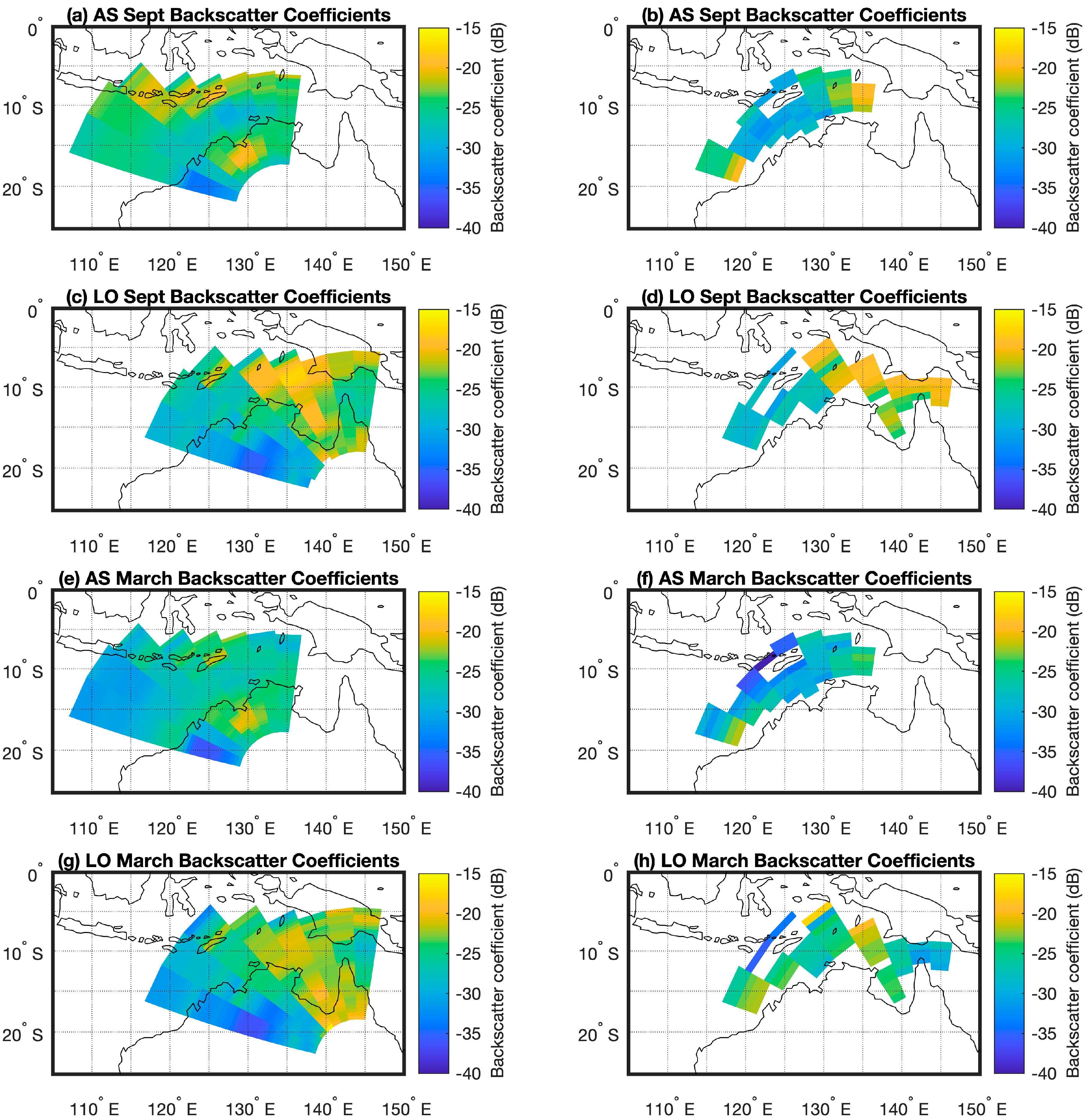
The daytime sea surface backscatter coefficient was calculated using the Barrick method (shown in Figure 5) and the backscatter ionogram method for September 2015 and March 2016. The monthly median backscatter coefficients calculated using the backscatter ionogram method for each range cell of the eight backscatter sounder beams are shown in Figure 6 (left). The corresponding monthly median sea surface backscatter coefficients for each range cell calculated using the Barrick method with the JONSWAP sea spectrum and the 10 arcminute resolution sea state data from the Centre for Australian Weather and Climate Research are shown in Figure 6 (right).
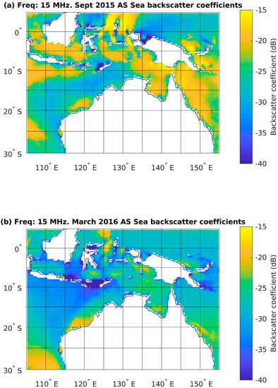
Figure 5.
Monthly daytime median sea surface backscatter coefficients calculated with the Barrick method using a radiowave frequency of 15 MHz for a radar located at Alice Springs in (a) September 2015 and (b) March 2016. The 0.4° resolution sea state data were used to calculate the JONSWAP spectrum.
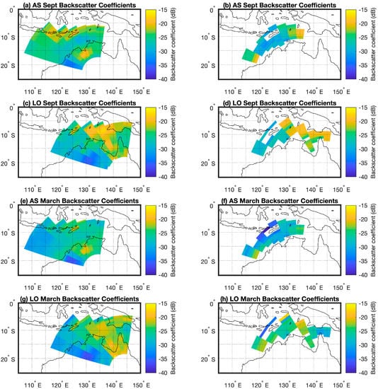
Figure 6.
Monthly median daytime backscatter coefficients calculated using the backscatter ionogram method (left) and Barrick method (right). Range-azimuth cells that contain some land areas were excluded from the calculation for the Barrick method.
A large difference between the sea surface backscatter coefficients from September 2015 and March 2016 was seen in the results from both methods. In general, the March sea surface backscatter coefficients were lower than the September sea surface backscatter coefficients. This was likely due to a calmer sea in March, providing less developed wave faces for radio waves to backscatter from. The backscatter coefficients in the Gulf of Carpentaria (13°S, 139°E) and the Arafura Sea (9°S, 136°E) were significantly larger in September 2015 when compared with March 2016. This difference between the months was observed in the Longreach results from both methods. The sea surface backscatter coefficients around the Lesser Sunda Islands (9°S, 120°E) were also larger in September than in March.
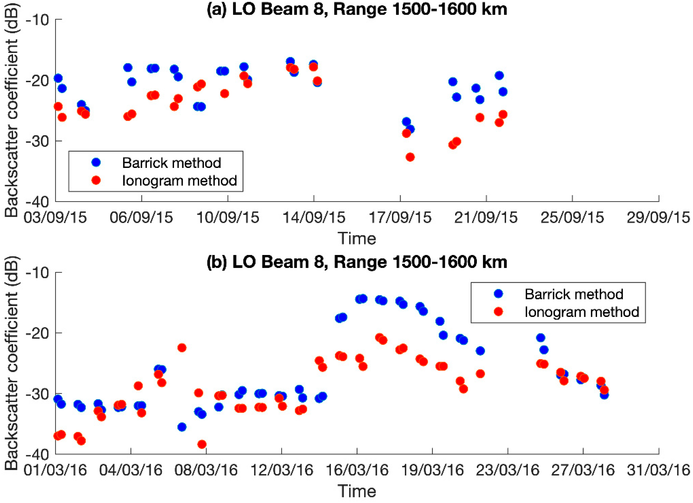
The sea surface backscatter coefficients from the Barrick method and ionogram method for a single range-azimuth cell for each morning and afternoon throughout September 2015 (top) and March 2016 (bottom) are shown in Figure 7. The two methods appear to agree relatively well, with the trends of lower and higher sea surface backscatter coefficients throughout the months agreeing. However, while the general trends were similar, there was a period from approximately the 16 to 21 March 2016 where the sea surface backscatter coefficients from the Barrick method were approximately 5 dB larger than the sea surface backscatter coefficients from the backscatter ionogram method.

Figure 7.
Backscatter coefficients calculated via the Barrick method (blue) and the backscatter ionogram method (red) for a single location (Longreach beam 8, at a range of 1500–1600 km) throughout (a) September 2015 and (b) March 2016.
The mean difference between the results from the two methods over these times was calculated for each of the range-azimuth cells of the backscatter sounders. The results are displayed in Figure 8. A cursory inspection of this figure indicates that while at some locations the two methods agree well, there are other locations where there are significant differences between the two methods. The Alice Springs ionogram backscatter coefficients (Figure 8a,b) tended to be slightly larger than those from the Barrick method. The mean difference between these two methods was similar across all beams and ranges investigated, although there did appear to be a slightly larger difference in the central beams than the edge beams. It is possible an azimuthal dependence may be introduced by deviations of the real antenna gain patterns from the idealised model antenna gain patterns used in the ionogram synthesis for the backscatter ionogram method.
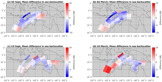
Figure 8.
Mean difference between the Barrick method and the backscatter ionogram method backscatter coefficients. The difference between the methods was calculated when data were available throughout a month, then the mean difference was calculated.
For Longreach (Figure 8c,d), the mean difference for each range-azimuth cell was relatively constant over all range-azimuth cells in September; the pattern appeared to be similar to Alice Springs with slightly larger differences in the central beams than the edge beams and again is attributed to possible deviations in the antenna pattern from the idealised model. However, during March, the backscatter ionogram method produced much lower backscatter coefficients than the Barrick method for the two western beams that look over the Indian Ocean (13°S, 122°E). However, while the sounder-derived sea surface backscatter coefficient is reduced in beams 1 and 2 during March, there is very little change in the sea surface backscatter coefficient derived from the sea state data using the Barrick method. This is not currently understood, and one possibility is that the sea state data in this region were in error during March 2016. This possibility is investigated in Section 4.
The RMS difference between the backscatter coefficients from the two methods was calculated for each sounder and month. This difference included all the data available for each range-azimuth cell and so was weighted towards the locations where data were available at more times. The RMS difference in the Alice Springs sea surface backscatter coefficients when the ionogram comparison results were subtracted from the wave spectrum results was 5.1 and 6.9 dB in September and March, respectively. The RMS difference between the two methods using data from all the Longreach range-azimuth cells was 4.2 and 6.3 dB in September and March, respectively.
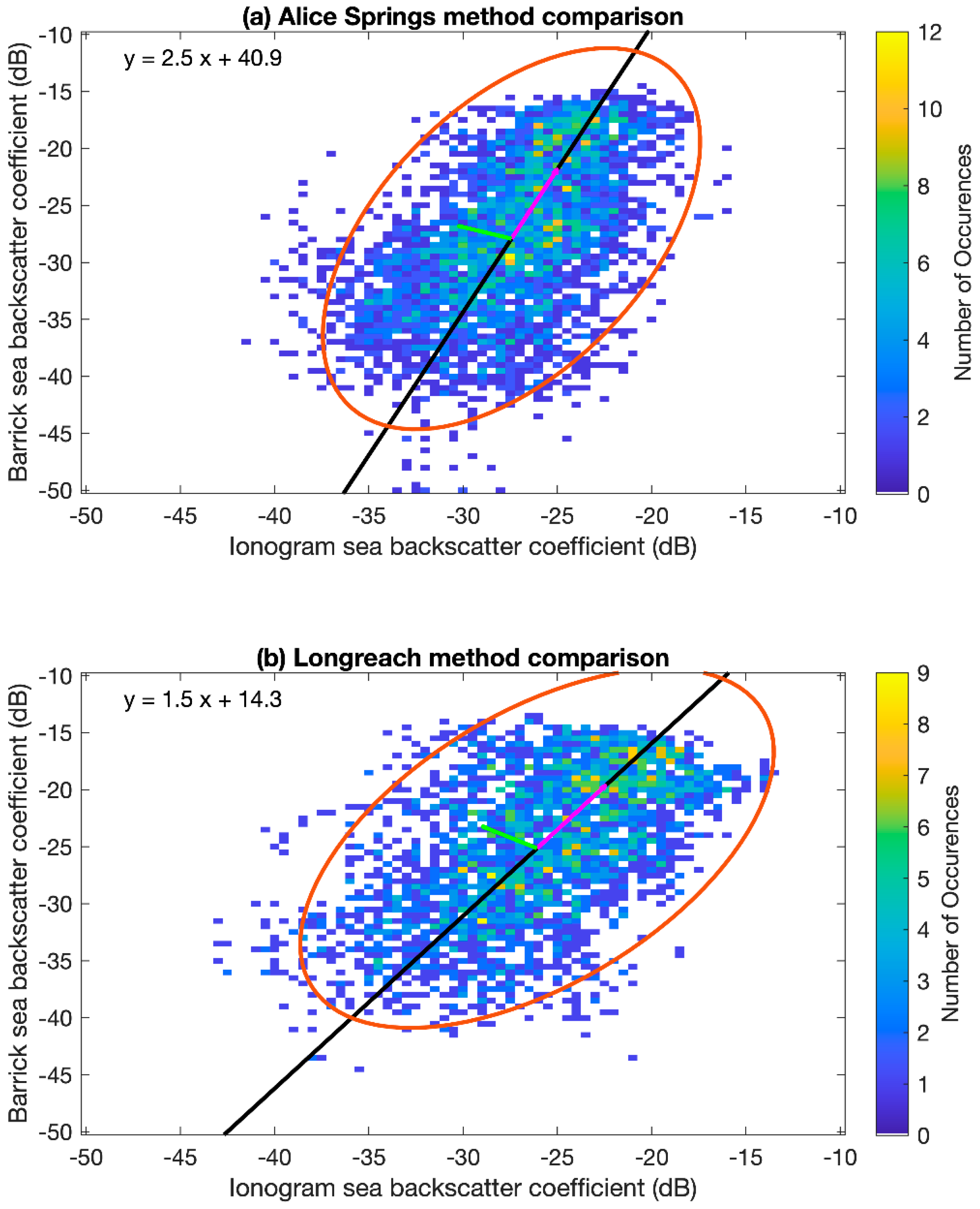
The backscatter coefficients for each method from all times in both September 2015 and March 2016 and all range-azimuth cells were plotted against each other as 2D histograms for each sounder (shown in Figure 9). The total number of data points in the Longreach histogram and the Alice Springs histogram are 2907 and 3457. If the two methods produced similar results, it is expected that these 2D histograms would show a linear relationship with a slope of one that passed through the origin. This linear trend could be seen, although the slopes and intercepts did not match this relationship.
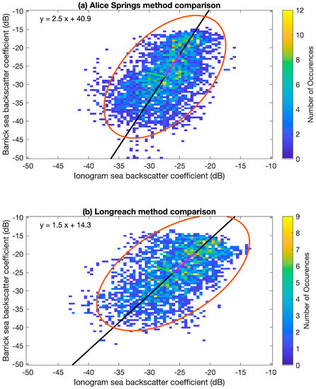
Figure 9.
(a) Alice Springs and (b) Longreach sea surface backscatter coefficients from both September 2015 and March 2016 calculated using the Barrick method with hindcast data vs. sea surface backscatter coefficients calculated using the backscatter ionogram method. A line of best fit is shown in black, with the corresponding equation in the top left corner and a 95% confidence error ellipse shown in red. The eigenvectors of the covariance matrix are shown in green and magenta. The centre of the ellipse for Alice Springs is at (−27.4 dB, −27.9 dB) and for Longreach is at (−26.1 dB, −25.1 dB).
A Pearson correlation test was conducted to test the linear correlation between the results from the Barrick and the backscatter ionogram methods. This tested the null hypothesis that there was no relationship observed between the results. The strength of the correlation is represented by the absolute value of the correlation coefficient and the direction by the sign of the correlation coefficient. The significance level was given by the P value. For these tests, the P values were less than 0.001, so the corresponding correlation coefficients were considered significant at greater than the 99% confidence interval. The correlation coefficients for Alice Springs and Longreach were 0.51 and 0.53, respectively. This indicates there is a moderate positive linear relationship in the results from the two methods of calculating the sea surface backscatter coefficient.
A line of best fit was fitted using an orthogonal least squares linear regression method (Figure 9). This method was chosen over a simple linear regression as errors in both the variables are considered, rather than using one variable to predict the other. For both sounders, the slope was greater than 1 and the intercept was positive which suggested differences between the two methods. The slope of the fitted line in the Alice Springs and Longreach results was 2.5 and 1.5, respectively. Using these fitted lines, the ionogram comparison and wave spectrum methods produced the same results when the backscatter coefficient was −27.3 and −28.6 dB for the Alice Springs and Longreach sounders, respectively. The slopes of both fitted lines were greater than one which suggested that the backscatter coefficients from the Barrick method had a greater dynamic range than those from the ionogram method.
A 95% confidence error ellipse was also plotted on the results (Figure 9). To create these error ellipses, it was assumed the data for each method were normally distributed. The orientation of the ellipse is determined by the covariance of the data and the magnitude of the axes of the ellipse are determined by the variance in the data (Table 1) [25]. The eigenvectors of the covariance data are plotted in green and magenta, these represent the direction of the most spread in the data and are aligned with the semi-major and semi-minor axes of the ellipse, while the eigenvalues define how large this spread is. The centre of the error ellipse for Alice Springs was at (−27.4 dB, −27.9 dB) and the centre of the error ellipse for Longreach was at (−26.1 dB, −25.1 dB). This shows that the two methods had good agreement for the values that were most common.

Table 1.
95% confidence error ellipse results. The centre of the ellipse is at (X0, Y0).
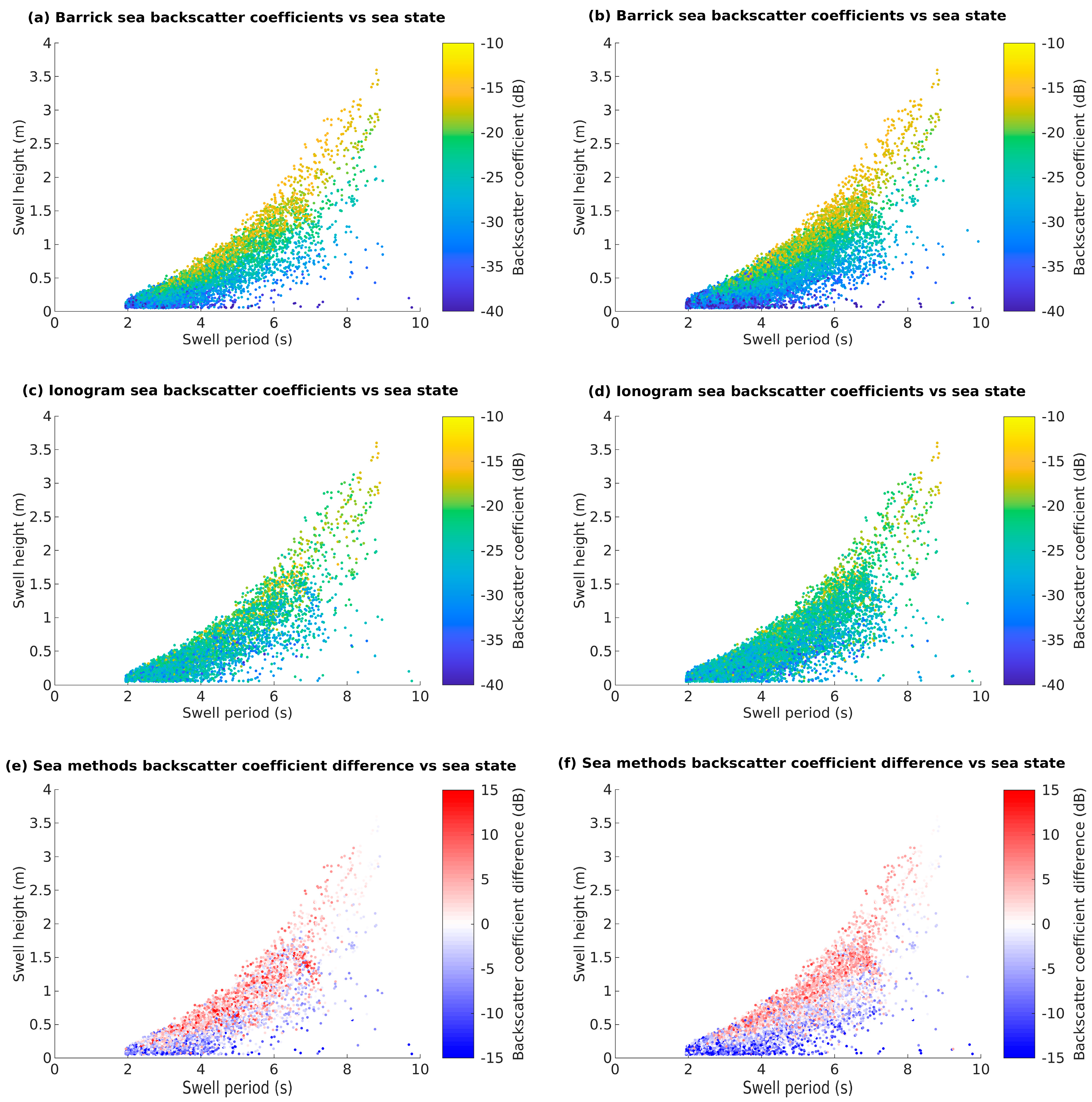
The effects of different sea conditions on the backscatter coefficients from the two methods were investigated using the significant swell height and the swell period of the wind sea from the hindcast sea data. Figure 10 shows the backscatter coefficient from the Barrick method (top panel), ionogram method (middle panel) and the difference between these methods (bottom panel) against the swell height and period for the Longreach (left) and Alice Springs (right) sounders. In general, the backscatter coefficient increased with increasing swell heights and decreasing swell periods. This trend is seen in both methods of calculating the sea surface backscatter coefficients. However, a greater range in the sea surface backscatter coefficients from the Barrick method is clearly seen. At a given swell period, the sea surface backscatter coefficients from the Barrick method are less than the ionogram method when calculated for small swell heights, and larger at larger swell heights.
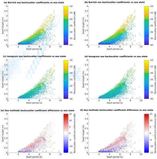
Figure 10.
Sea surface backscatter coefficients vs. sea state using data from September 2015 and March 2016 for Longreach (left) and Alice Springs (right).
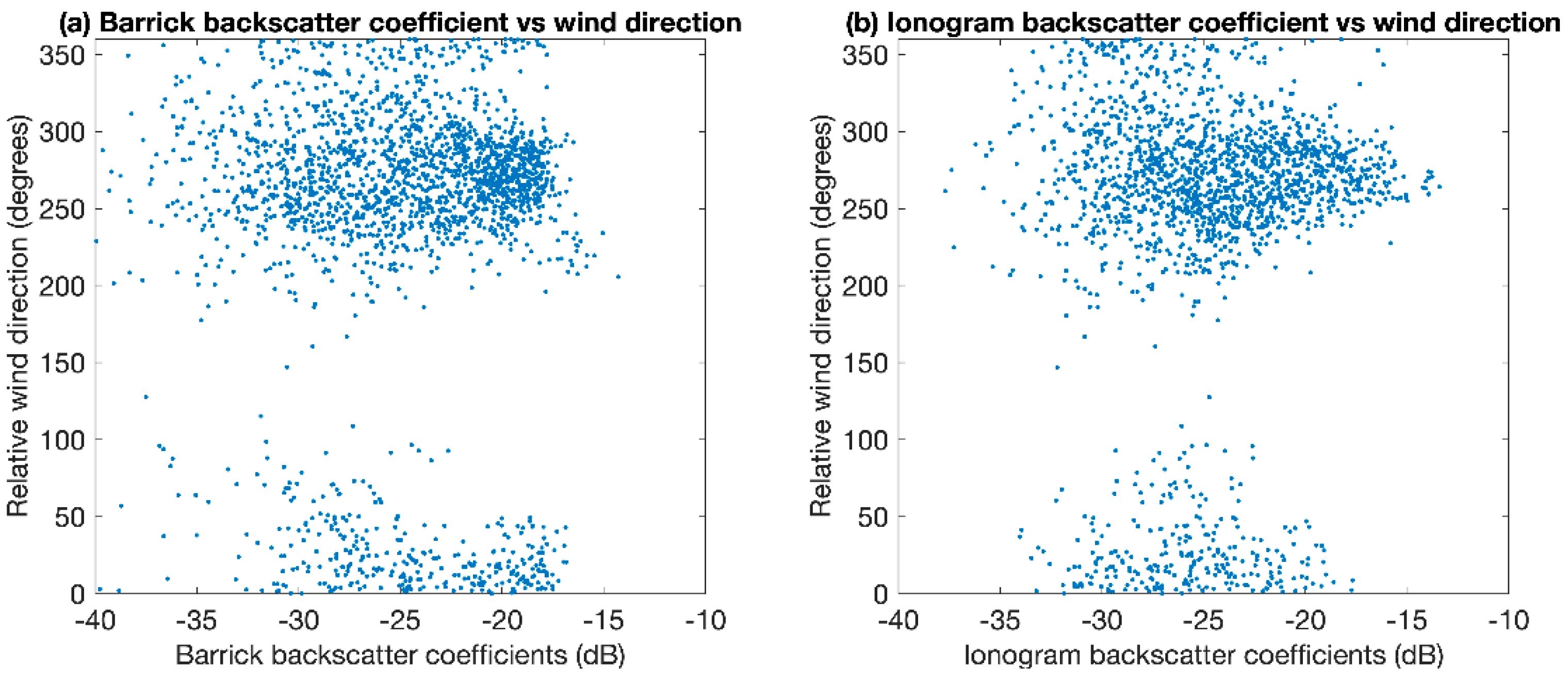
The effect of the relative wind direction, defined as the angle between the radar observation azimuth and the wind direction, on the sea surface backscatter coefficients was also investigated. Gardiner-Garden [17] showed that under a fully developed sea, the backscatter coefficient changes weakly under changes in wind direction. Figure 11 shows the backscatter results for Longreach September 2015 plotted against the relative wind direction. Little correlation was seen between the backscatter coefficient and the relative wind direction. The swell height and period influence the backscatter coefficient, as seen in Figure 10, which potentially obscures any correlation with the relative wind direction.
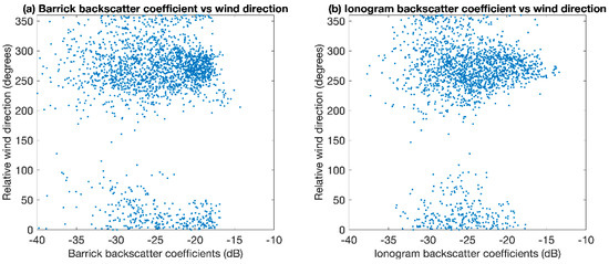
Figure 11.
Backscatter coefficients from the Barrick method (left) and ionogram method (right) for Longreach September 2015 versus the relative wind direction.
4. Discussion
It was expected that the results from the two methods would differ due to the many models and assumptions used in each method. Variance and errors in the results from the backscatter ionogram method are likely to be introduced by errors in the real-time ionospheric model, the model of the antenna gains and the George and Bradley ionospheric absorption model, which is climatological rather than real time. Biases in the backscatter sounder measurements due to inaccurate modelling of transmit power, signal processing losses and instrumental losses, such as the antennae and cabling, may also introduce errors. The resolution of the power in the observed backscatter ionograms was 0.5 dB, so differences in the results no smaller than this were expected. The use of two-dimensional numerical ray tracing instead of three-dimensional ray tracing may also introduce variance due to the effects of out of plane propagation from ionospheric tilts and ray splitting into the ordinary and extraordinary propagation modes being disregarded. However, these effects are expected to be small as the range-azimuth cell size is much larger than the differences introduced to the location of where the modelled rays come to ground. The limitations of this method are discussed in more detail in Edwards et al. [4].
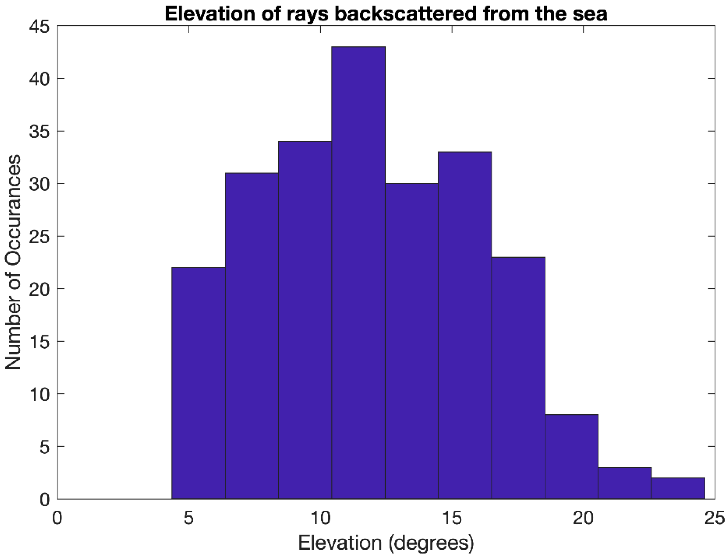
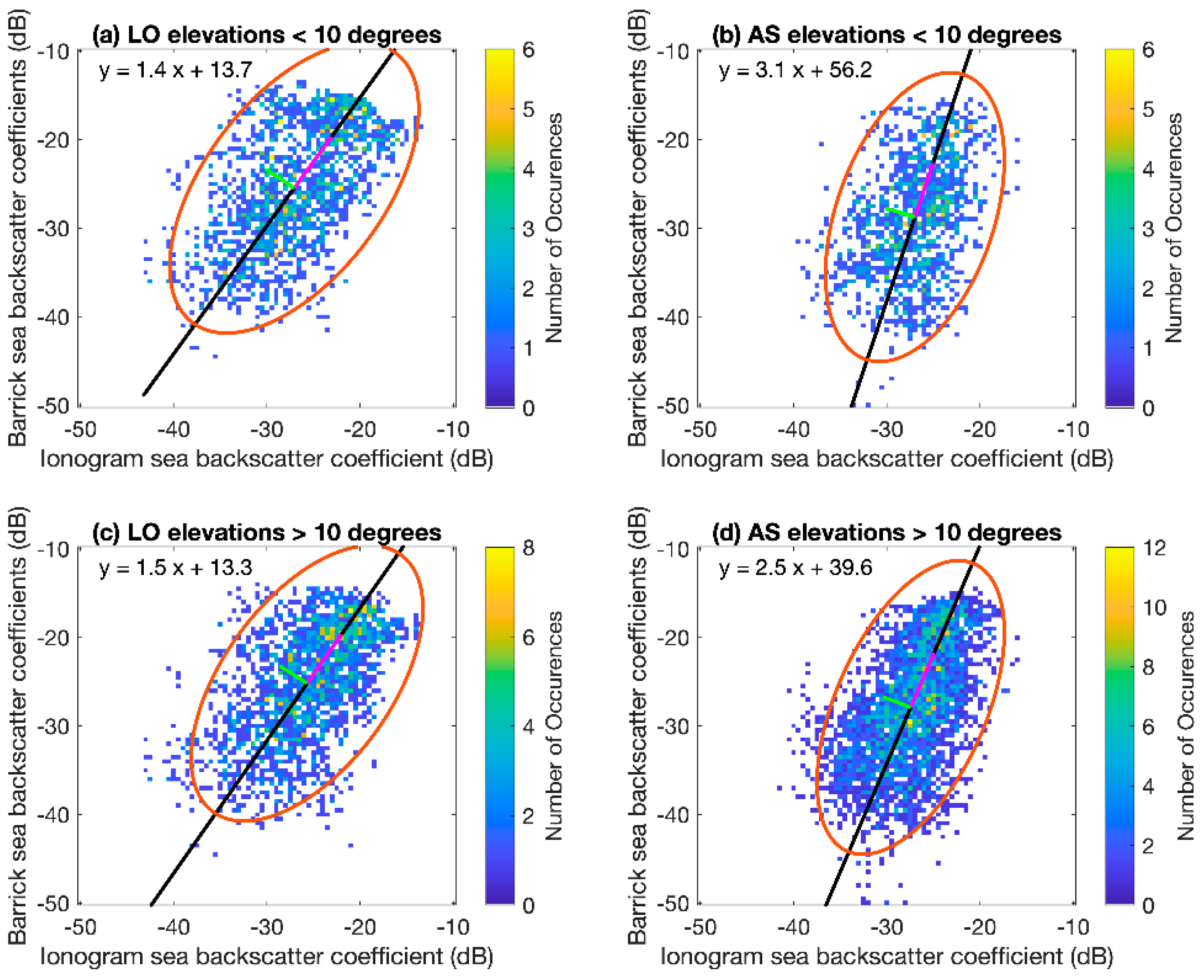
To utilize the Barrick method of calculating sea surface backscatter coefficient, several different models combined with appropriate assumptions were required. Only first-order Bragg scatter was considered in the Barrick method, higher-order scatter was ignored. It was assumed the water was deep, so the model may not be valid in coastal regions where the ocean waves interact with the ocean floor. Lipa, Nyden, Barrick and Kohut [11] showed there was increased sea surface backscatter from shallow water as the radar spectrum saturated at smaller wave heights. It was also assumed that the radio waves were at grazing incidence angles, which is not always the case for sky wave radar. The effects of shadowing between waves at grazing incidence angles are implicitly included in the measured backscatter coefficients from the ionogram method. However, we only considered first-order effects when calculating the backscatter coefficients from the Barrick theory. Second-order effects were not included as they are 20–30 dB lower than the first-order Bragg scatter [26]. A histogram of the elevations of the rays backscattered from the sea, produced from the raytracing for the model backscatter ionograms, is shown in Figure 12. The elevation of the backscattered radio waves typically decreases with increasing range from the radar and the mean ray elevation was 12 degrees, which is larger than grazing angles (elevations < 10 degrees). For rays backscattered from the sea near the radar, the elevation angle was up to 25 degrees. It is expected that the backscatter coefficient increases with increasing radio wave elevation [9], and this effect is more pronounced for smooth surfaces [27]. Scatter plots of the backscatter coefficient results from the Barrick versus the ionogram method for rays with elevations less than and greater than 10 degrees were created (shown in Figure 13). Backscatter coefficients obtained from rays with elevation less than 10 degrees are shown in Figure 13a,b and backscatter coefficients obtained from rays with elevations greater than 10 degrees are shown in Figure 13c,d. There was little difference between the results from rays with elevations near grazing and rays with larger elevations, at a given location.

Figure 12.
Histogram of the mean elevation of the rays reaching each range-azimuth cell for Alice Springs and Longreach in September 2015 and March 2016. The mean value is 12 degrees.

Figure 13.
Scatter plots of the sea surface backscatter coefficients from the Barrick versus the ionogram method for rays with (top) elevations less than 10 degrees and (bottom) elevations greater than 10 degrees. A line of best fit is shown in black, with the corresponding equation in the top left corner and a 95% confidence error ellipse shown in red. The eigenvectors of the covariance matrix are shown in green and magenta.
Limitations of the JONSWAP spectrum and the sea state data used to generate this spectrum would also introduce errors into the sea surface backscatter coefficients from the Barrick method. The JONSWAP wave spectrum assumed that a wind with a constant velocity had been blowing over the ocean for long periods of time. This allowed a relatively simple spectrum to be calculated. However, it was not necessarily representative of a typical ocean wave spectrum where local winds may create multiple peaks. The accuracy of the hindcast sea state data is dependent on the forcing wind model. The WAVEWATCH III model was forced with surface winds from climate forecast system reanalysis data at 0.3 degrees spatial and hourly temporal resolution [14]. Imprecise modelling of the effects of small islands and bottom interactions near coastlines can reduce the validity of the generated hindcast data. Figure 14, obtained from Hemmer et al., shows the mean bias in the significant wave height from hindcast data when compared with satellite altimeter data from 1985 to 2012. Notable biases near the coastlines, especially over the Great Barrier Reef (18°S, 148°E), will also cause some error in the backscatter coefficient calculated using the data in these areas.
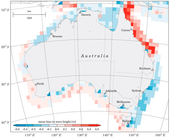
Figure 14.
Spatial variability of the mean bias of the modelled significant wave height (Hs in units of m) relative to observations from altimeters (hindcast model minus altimeter). Figure obtained from Hemer, et al. [28].
In our area of interest, the bias in the wave heights is generally negative. Accounting for this bias, assuming there is no bias in the other hindcast parameters such as the wave period and wind direction, would increase the backscatter coefficients calculated using the Barrick method, as seen in Figure 2. The effect of this bias on the scatter plots comparing the results from the two methods, shown in Figure 9, was investigated. The Alice Springs results were recreated adjusting for a constant negative bias of 0.2 m in the significant wave height of the primary, secondary, tertiary and wind swells, while all other hindcast parameters were unchanged. The resulting scatter plot of the Barrick versus the ionogram sea surface backscatter coefficients when this bias was accounted for is shown in Figure 15. The slope of the line of best fit is 2.0, which is less than the slope of 2.5 from Figure 9 when no bias was included. This simple adjustment to the data used by the Barrick method improved the slope of the line of best fit.
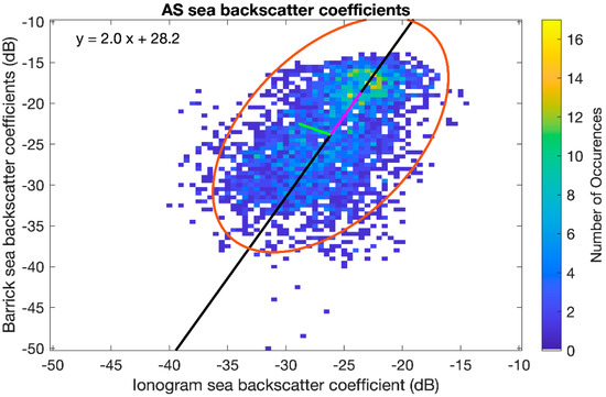
Figure 15.
Scatter plot of the Alice Springs sea surface backscatter coefficients from the Barrick method accounting for a wave height bias of −0.2 m versus the ionogram method using data from September 2015 and March 2016. A line of best fit is shown in black, with the corresponding equation in the top left corner and a 95% confidence error ellipse shown in red. The eigenvectors of the covariance matrix are shown in green and magenta.
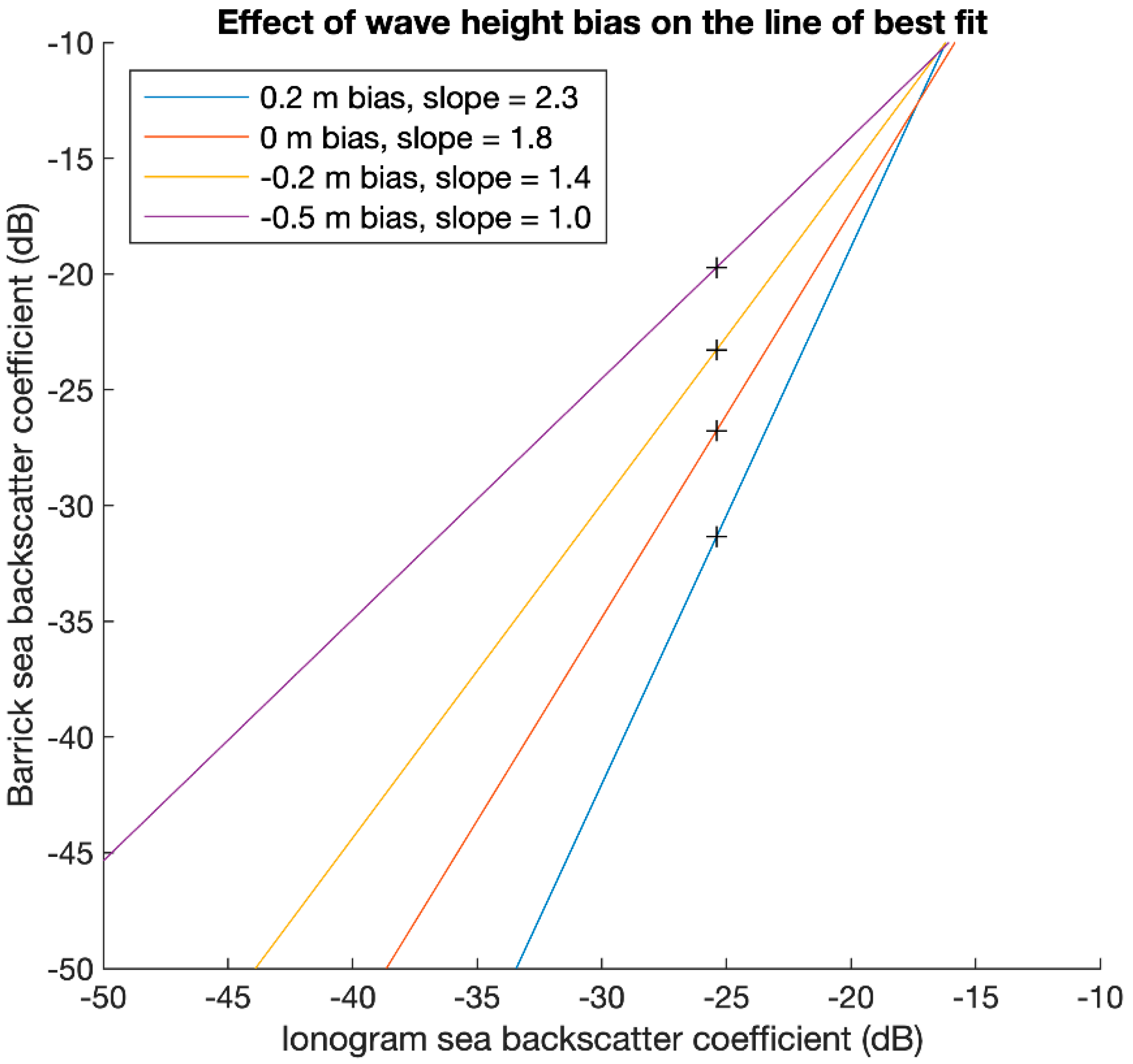
The effect of the wave height bias on the Barrick method of calculating sea surface backscatter coefficients was further investigated by examining a range of bias values. The mean primary, secondary, tertiary, and wind swell significant wave heights over the Alice Springs field of view in September 2015, with no bias applied, were 0.53 m, 0.25 m, 0.16 m, and 0.58 m, respectively. Lines of best fit for scatter plots of the Barrick results versus the ionogram results for September 2015 with biases of 0.2 m, 0 m, −0.2 m, and −0.5 m considered are shown in Figure 16. If an applied bias resulted in a negative swell height, that swell height was set to 0 m. There were relatively large changes in the slopes of the lines of best fit when these likely values for the wave height bias (as seen in Figure 14) were accounted for. This suggests that the differences noted earlier between the results from the Barrick method and the ionogram method may largely be due to biases in the sea state data generated from the WAVEWATCH III model. The centres of the error ellipses (X0, Y0) are also shifted by biases in the wave height. As there is no change in the data from the ionogram method, X0 remains at −25.4 dB; however, Y0 shifts upwards as negative biases in the data are accounted for (wave heights are increased). The values of Y0 obtained when a bias in the wave height of 0.2, 0, −0.2, and −0.5 m is accounted for are −31.4, −26.8, −23.3 and −19.7 dB, respectively. Finally, we note that other biases in sea state parameters such as the wave period and direction used to define the JONSWAP spectrum may have a further effect on the results. However, as we do not have knowledge of these potential biases, it is beyond the scope of this paper to consider this further.

Figure 16.
Effect of accounting for various potential wave height biases in the sea state data used for the Barrick method on the line of best fit for the Alice Springs September 2015 Barrick versus the ionogram sea surface backscatter coefficients. The + symbols are at the centre of the error ellipses associated with each line.
5. Conclusions
An understanding of the sea surface backscatter coefficient is important for assessing over-the-horizon radar performance and for remote sensing of the sea state. This paper outlined two methods of calculating sea surface backscatter coefficients: the Barrick and backscatter ionogram methods. Sea surface backscatter coefficients were calculated for September 2015 and March 2016. It was found that the sea surface backscatter coefficients from each method followed similar trends over time, with periods of low and high sea surface backscatter coefficients agreeing. In general, the values for the sea surface backscatter coefficients calculated with each method were also similar; however, it was noted there was a greater range in the sea surface backscatter coefficients from the Barrick method. Due to the many different models and assumptions that were used with each method, it was expected there would be some differences between the results. It is likely that biases in the sea state data generated from the WAVEWATCH III model contributed significantly to the differences between the ionogram and the Barrick methods.
To further understand the effects of the different models on the backscatter coefficient, the results of the Barrick method when used with other wave height spectra could be investigated. A comparison of these two methods against some truth data is required to better understand the differences and when each method is suitable to use. This may be possible by
- Using a buoy to obtain the wave height spectrum for a particular location at a given time to be used with the Barrick method;
- Using a transponder located near the coast to more accurately obtain a measurement of the ionospheric absorption experienced by the modelled rays in the backscatter ionogram method;
- Comparing the results from these methods with surface wave radar measurements.
Author Contributions
Conceptualization, D.E., M.C. and A.M.; methodology, D.E. and M.C.; software, D.E. and M.C.; validation, D.E., M.C. and A.M.; formal analysis, D.E.; investigation, D.E.; resources, D.E., M.C. and A.M.; data curation, D.E.; writing—original draft preparation, D.E.; writing—review and editing, D.E., M.C. and A.M.; visualization, D.E.; supervision, M.C. and A.M.; project administration, D.E., M.C. and A.M. All authors have read and agreed to the published version of the manuscript.
Funding
This research was supported by Defence Science and Technology Group and The University of Adelaide. We acknowledge the support we have received for this research through the provision of an Australian Government Research Training Program Scholarship.
Data Availability Statement
Backscatter sounder data and real-time ionospheric model data are owned by the Australian Commonwealth Government, Department of Defence. They may be made available on a case-by-case basis pursuant to Defence Science and Technology Group policy for public release of information by contacting the primary author. The sea hindcast dataset used for this research is available in this in-text data citation reference: Durrant et al. [13] [Creative Commons Attribution-ShareAlike 4.0 International License].
Acknowledgments
The authors acknowledge Trevor Harris and David Holdsworth for useful discussions and suggestions. Results were obtained using the HF propagation toolbox, PHaRLAP, developed by Defence Science and Technology Group, Australia. This toolbox is available from https://www.dst.defence.gov.au/opportunity/pharlap-provision-high-frequency-raytracing-laboratory-propagation-studies (accessed on 22 February 2021).
Conflicts of Interest
The authors declare no conflict of interest.
References
- Barrick, D.E. Near-grazing illumination and shadowing of rough surfaces. Radio Sci. 1995, 30, 563–580. [Google Scholar] [CrossRef]
- Crombie, D.D.; Watts, J.M. Observations of coherent backscatter of 2–10 MHz radio surface waves from the sea. Deep-Sea Res. Oceanogr. Abstr. 1968, 15, 81–87. [Google Scholar] [CrossRef]
- Lipa, B.J.; Barrick, D.E. Extraction of sea state from HF radar sea echo: Mathematical theory and modeling. Radio Sci. 1986, 21, 81–100. [Google Scholar] [CrossRef]
- Edwards, D.; Cervera, M.; MacKinnon, A. High Frequency Land Backscatter Coefficients over Northern Australia and the Effects of Various Surface Properties. IEEE Trans. Antennas Propag. 2022. [Google Scholar] [CrossRef]
- Edwards, D.J. High Frequency Surface Backscatter Coefficients; University of Adelaide: Adelaide, Australia, 2020. [Google Scholar]
- Munk, W.H.; Nierenberg, W.A. High Frequency Radar Sea Return and the Phillips Saturation Constant. Nature 1969, 224, 1285. [Google Scholar] [CrossRef]
- Barrick, D.; Snider, J. The statistics of HF sea-echo Doppler spectra. IEEE J. Ocean. Eng. 1977, 2, 19–28. [Google Scholar] [CrossRef]
- Rice, S.O. Reflection of electromagnetic waves from slightly rough surfaces. Commun. Pure Appl. Math. 1951, 4, 351–378. [Google Scholar] [CrossRef]
- Barrick, D. First-order theory and analysis of MF/HF/VHF scatter from the sea. IEEE Trans. Antennas Propag. 1972, 20, 2–10. [Google Scholar] [CrossRef] [Green Version]
- Parkinson, M.L. Advanced directional sea spectrum studies with the Bribie Island MF/lower HF surface-wave radar. Radio Sci. 1994, 29, 815–830. [Google Scholar] [CrossRef]
- Lipa, B.; Nyden, B.; Barrick, D.; Kohut, J. HF Radar Sea-echo from Shallow Water. Sensors 2008, 8, 4611–4635. [Google Scholar] [CrossRef] [PubMed]
- Hasselmann, K.; Barnett, T.; Bouws, E.; Carlson, H.; Cartwright, D.; Enke, K.; Ewing, J.; Gienapp, H.; Hasselmann, D.; Kruseman, P.; et al. Measurements of wind-wave growth and swell decay during the Joint North Sea Wave Project (JONSWAP). Deut. Hydrogr. Z. 1973, 8, 1–95. [Google Scholar]
- Neller, C. Over-the-Horizon Radar Sea-State Parameter Estimation Using Bureau of Meteorology Interactive Weather and Wave Forecast Data; DSTO-DP-1266; NSID, DST Group: Canberra, Australia, 2014.
- Durrant, T.H.; Greenslade, D.J.M.; Hemer, M.A.; Trenham, C.E. A Global Wave Hindcast Focussed on the Central and South Pacific; Centre for Australian Weather and Climate Research: Melbourne, Australia, 2014.
- Barrick, D.E.; Peake, W.H. A Review of Scattering from Surfaces with Different Roughness Scales. Radio Sci. 1968, 3, 865–868. [Google Scholar] [CrossRef]
- Barrick, D.E.; Headrick, J.M.; Bogle, R.W.; Crombie, D.D. Sea backscatter at HF: Interpretation and utilization of the echo. Proc. IEEE 1974, 62, 673–680. [Google Scholar] [CrossRef]
- Gardiner-Garden, R.S.; Pincombe, A.H. A Study of the Seasonal Pattern of Variability in the HF Radar Cross-Section of the Sea; Intelligence, Surveillance and Space Division, DST Group: Canberra, Australia, 1996.
- Brodtkorb, P.A.; Johannesson, P.; Lindgren, G.; Rychlik, I.; Rydén, J.; Sjö, E. WAFO—A Matlab Toolbox for Analysis of Random Waves and Loads. In Proceedings of the Tenth International Offshore and Polar Engineering Conference, Seattle, WA, USA, 28 May–2 June 2000. [Google Scholar]
- Gardiner-Garden, R.; Cervera, M.; Debnam, R.; Harris, T.; Heitmann, A.; Holdsworth, D.; Netherway, D.; Northey, B.; Pederick, L.; Praschifka, J.; et al. A description of the Elevation sensitive Oblique Incidence Sounder Experiment (ELOISE). Adv. Space Res. 2019, 64, 1887–1914. [Google Scholar] [CrossRef]
- Cervera, M.A.; Harris, T.J. Modeling ionospheric disturbance features in quasi-vertically incident ionograms using 3-D magnetoionic ray tracing and atmospheric gravity waves. J. Geophys. Res. Space Phys. 2014, 119, 431–440. [Google Scholar] [CrossRef]
- Barnes, R.; Gardiner-Garden, R.; Harris, T. Real Time Ionospheric Models for the Australian Defence Force. 2000; pp. 122–135. Available online: https://web.archive.org.au/awa/20040915175538mp_/http://pandora.nla.gov.au/pan/33010/20030801-0000/www.ips.gov.au/IPSHosted/NCRS/wars/wars2000/commg/barnes.pdf (accessed on 22 February 2021).
- George, P.L.; Bradley, P.A. Relationship between H.F. absorption at vertical and oblique incidence. Proc. Inst. Electr. Eng. 1973, 120, 1355–1361. [Google Scholar] [CrossRef]
- George, P.L.; Bradley, P.A. A new method of predicting the ionospheric absorption of high frequency waves at oblique incidence. Telecommun. J. 1974, 41, 307–312. [Google Scholar]
- Burke, G.; Poggio, A.; Logan, J.; Rockway, J. NEC—Numerical electromagnetics code for antennas and scattering. In Proceedings of the 1979 Antennas and Propagation Society International Symposium, Seatlle, WA, USA, 18–22 June 1979; pp. 147–150. [Google Scholar]
- Ogundare, J.O. Understanding Least Squares Estimation and Geomatics Data Analysis; John Wiley & Sons, Incorporated: Newark, HJ, USA, 2018. [Google Scholar]
- Skolnik, M.I. Radar Handbook, 3rd ed.; McGraw-Hill: New York, NY, USA, 2008; pp. 20–31. [Google Scholar]
- Ulaby, F.T.; Batlivala, P.P.; Dobson, M.C. Microwave Backscatter Dependence on Surface Roughness, Soil Moisture, and Soil Texture: Part I-Bare Soil. IEEE Trans. Geosci. Electron. 1978, 16, 286–295. [Google Scholar] [CrossRef]
- Hemer, M.A.; Zieger, S.; Durrant, T.; O’Grady, J.; Hoeke, R.K.; McInnes, K.L.; Rosebrock, U. A revised assessment of Australia’s national wave energy resource. Renew. Energy 2017, 114, 85–107. [Google Scholar] [CrossRef]


Publisher’s Note: MDPI stays neutral with regard to jurisdictional claims in published maps and institutional affiliations. |
© 2022 by the authors. Licensee MDPI, Basel, Switzerland. This article is an open access article distributed under the terms and conditions of the Creative Commons Attribution (CC BY) license (https://creativecommons.org/licenses/by/4.0/).