Assessment of VIIRS on the Identification of Harmful Algal Bloom Types in the Coasts of the East China Sea

Abstract

Visible Infrared Imaging Radiometer Suite (VIIRS) data were systematically evaluated and used to detect harmful algal bloom (HAB) and classify algal bloom types in coasts of the East China Sea covered by optically complex and sediment-rich waters. First, the accuracy and spectral characteristics of VIIRS retrieved normalized water-leaving radiance or the equivalent remote sensing reflectance from September 2019 to October 2020 that were validated by the long-term observation data acquired from an offshore platform and underway measurements from a cruise in the Changjiang Estuary and adjacent East China Sea. These data were evaluated by comparing them with data from the Moderate-Resolution Imaging Spectroradiometer. The bands of 486, 551, and 671 nm provided much higher quality than those of 410 and 443 nm and were more suitable for HAB detection. Secondly, the performance of four HAB detection algorithms were compared. The Ratio of Algal Bloom (RAB) algorithm is probably more suitable for HAB detection in the study area. Importantly, although RAB was also verified to be applicable for the detection of different kinds of HAB (Prorocentrum donghaiense, diatoms, Ceratium furca, and Akashiwo sanguinea), the capability of VIIRS in the classification of those algal species was limited by the lack of the critical band near 531 nm.

1. Introduction

The Visible Infrared Imaging Radiometer Suite (VIIRS) is the new generation of medium resolution image radiometer of the United States, which combines most features of its predecessor, such as the Moderate-resolution Imaging Spectroradiometer (MODIS). It has nine visible/infrared bands with an average bandwidth of 20 nm, twelve mid-far infrared bands, and one day/night band, among which only five bands have a spatial resolution of 375 m and the spatial resolution of the remaining bands is 750 m [1,2,3,4]. VIIRS is mainly used to monitor the radiation changes in ocean, atmosphere, ice, and land in visible and infrared bands, and provide data for monitoring ocean color, ocean surface temperature, and other surface changes [4,5,6,7,8]. The first VIIRS onboard Suomi National Polar-orbiting Partnership (SNPP) was successfully launched into an 824-km sun synchronous polar orbit on 28 October 2011; subsequently, the first Joint Polar Satellite System (JPSS-1) satellite launched into space on 18 November 2017 with VIIRS. In December 2017, JPSS-1 renamed NOAA-20 (hereinafter referred to as NA20). Both SNPP and NA20 are currently in stable operation [1,3]. After considerable community effort in sensor calibration and algorithm development, VIIRS has been shown to yield generally consistent data products for the global oceanic waters [4,9], and validation in coastal waters for VIIRS and MODIS reflectance data has been carried out in a few regions such as the Gulf of Mexico and South Atlantic Bight [10,11]. However, VIIRS is not equipped with some explicit MODIS bands, such as the terrestrial band at 531 nm and fluorescence band at 678 nm, as well as that in some standard VIIRS Level-2 products (such as the US National Aeronautics and Space Administration (NASA) L2GEN), and the remote sensing reflectance (R_rs) data from land band near 640 nm is not generated. The lack of these band data should limit capacity of VIIRS in coastal regions, which should be carefully assessed.

Currently, the MODIS sensors, as the predecessor of VIIRS, have been widely used for the detection, monitoring, and classification of Harmful Algal bloom (HAB) in coastal oceans around the world [12,13,14,15,16]. Whether VIIRS can continue the algal bloom monitoring capability of MODIS needs to be verified because the number of visible band settings in VIIRS is less than in MODIS, with the lack of, especially, the 531 nm band and chlorophyll fluorescence waves near 678 nm being problematic. For instance, in Colored Dissolved Organic Matter (CDOM) rich waters off southwest Florida, fluorescence line height (FLH) data of MODIS provided unique information that has been used to differentiate the toxic dinoflagellate, Karenia brevis (K. brevis), bloom [17]. Similarly, the backscattering/chlorophyll-a (Chl-a) ratio and Spectral Shape index at 486 nm (SS (486)) combined with the shape index in the 671 nm band (CI_MODIS) were used to differentiate K. brevis blooms [15,18,19]. The red-band difference technique was combined with the K. brevis bloom index to differentiate K. brevis bloom from other ones [20]. The success of these methods is obviously attributed to the use of the fluorescence band. Thus, it is indicated that VIIRS could not discriminate these high-phytoplankton water patches within the dark water due to its lack of a fluorescence band [21].

Aside from the CDOM-rich Florida coasts, the same success was also achieved in application of MODIS land bands (at 531 and 645 nm) to synoptically detect and characterize HAB in the optically complex coastal waters of northeast Asian, particularly in the sediment-rich coasts of the East China Sea (ECS) [22,23,24]. Noticeably, recent studies in these areas have been largely extended to the discrimination of the types or causative species of phytoplankton blooms. A novel MODIS-based method was developed to distinguish Karenia mikimotoi blooms from other types of blooms in the Seto Inland Sea of Japan, which is based on the spectral-slope difference of normalized water-leaving radiance [24]. Additionally, a new bio-optical algorithm based on backscattering feature at 555 nm and spectral shape near 645 nm was used to differentiate harmful raphidophyte Chattonella spp. blooms from diatom ones in the Ariake Sea, Japan [25]. Based on two MODIS band ratios, R_rs(555)/R_rs (531) and R_rs(488)/R_rs(443), it is possible to optically discriminate Cochlodinium polykrikoides blooms from non-dinoflagellate blooms in Korean coasts [26]. Similarly, in the ECS, a novel MODIS-based method using a Bloom Index, FLH, and total absorption coefficient at 443 nm (a(443)) was first proposed to distinguish these two bloom groups according to the spectral dissimilarities which can be characterized by the MODIS 443, 488, 531, and 555 bands [27]. In addition to this, two MODIS land bands were used to define two indices, a Prorocentrum donghaiense index (PDI) and a diatom index (DI), for discriminating P. donghaiense from diatom blooms [28]. It can be clearly found that these successes were primarily attributed to the use of land bands; however, further research is needed to confirm whether VIIRS, which lacks characteristic terrestrial and fluorescence bands, can classify algal species. Currently, the 638 nm terrestrial band has been used in the Multi-Sensor Level-1 to Level-2 (MSL12) algorithm for providing optical, biological, and geochemical characteristics of turbid nearshore and inland waters [6], but reflectance of this band is not generated in NASA’s standard L2 products. In addition, although a Red-Green-Chlorophyll-a Index (RGCI) was proposed to overcome its deficiency in CDOM-rich waters [21], the capacities of VIIRS to detect HAB in sediment-rich coasts still remains unclear. Furthermore, whether or not the absence of these bands limits the VIIRS application in discriminating bloom types also needs to be investigated.

Therefore, in this study, we evaluated VIIRS data in bloom type detection and selected the ECS coasts as the study area. This assessment involves three main objectives. The first is to validate R_rs data products from VIIRS (both MSL12 and L2GEN processing) when compared to Moderate Resolution Imaging Spectroradiometer of Aqua (MODISA; L2GEN processing only) and in situ datasets, since the reliability of operational monitoring of algal blooms primarily depends on the degree of the quantification of R_rs products. Second is to compare different bloom detection methods using VIIRS data in coasts of the ECS. The last but the most important is to evaluate the capabilities of VIIRS data in the discrimination of various bloom types, such as P. donghaiense and diatoms, along with other blooms.

2. Data and Methods

2.1. Study Area and In Situ Measurements

The study area covers most areas of the ECS (26–33°N, 119–126°E), including the Yangtze River Estuary (YRE) and the coasts of Shanghai Municipality and Zhejiang Province (Figure 1). Most of the coastal ocean has a depth of less than 50 m and is influenced by the Yangtze River plume, the Taiwan Strait Warm Current, the Kuroshio Current, and the coastal current along the Zhejiang coast [29,30]. Some of algal bloom records for the time of occurrence, location, and causative species were obtained from the Wenzhou Marine Environmental Monitoring Center Station (WMEMC) of State Oceanic Administration. These records cover the period from April to May 2020. Other records come from field measurements carried out during the cruise of Project of Long-term Observation and Research Plan in the Changjiang Estuary and Adjacent East China Sea (LORCE) in July 2013, August 2020, and August 2021. At each bloom station, 1 L or 500 mL water samples collected from Niskin bottles on the surface (2–3 m depth) were fixed with formalin to a final concentration of 2%. After at least 24 h of sedimentation, preserved samples were concentrated to 10–50 mL by slowly siphoning off the supernatant [31,32]. Subsequently, the concentrated samples were transferred into a 0.1 mL scaled slide using a pipette. The phytoplankton taxa were identified and counted on the entire slide using light microscopes (Leica DM2500 and DM6B) at 200×, 400×, or 630× magnification. At least 300 units (individual cells or colonies) were counted for each sample. All the collection, sedimentation, species identification, and abundance calculation of phytoplankton samples were performed complying with the Chinese National Standard [33].

Moreover, a fixed oceanographic platform called Dongou was used to collect a long-term series of radiometric measurements (such as R_rs and normalized water-leaving radiance (L_wn)). This platform was located in the southern part of the ECS (27.675°N and 120.358°E) at approximately 80 km southeast of Wenzhou in an area that minimized the adjacency effects in satellite data. In addition, the water depth around the platform was around 50 m, so that the bottom effects in L_wn were negligible. This oceanographic platform, owned and operated by WMEMC, has served as an offshore laboratory since 2017 and is an excellent site supporting ocean color validation activities through a comprehensive collection of bio-optical data. On this offshore platform, a Sea-Viewing Wide Field-of-View Sensor Photometer Revision for Incident Surface Measurements (SeaPRISM) autonomous radiometer system was deployed; its sea-viewing measurement sequence was executed every 30 min from 08:00 to 16:00 local time. The system collected water surface and sky radiation data; after processing to obtain L_wn data, it divided by the mean extraterrestrial solar irradiance (F₀) of the corresponding waveband to obtain R_rs data. The SeaPRISM system configuration performed ocean color measurements at 11 wavelengths from 400–1020 nm. The SeaPRISM data used in this study were collected during September 2019 to October 2020 and were manually checked to make sure that no corrupted spectra were present in this dataset. Only the L_wn and R_rs data at 412, 442, 490, 560, and 667 nm center wavelengths were used for the match-up comparison analysis with VIIRS. The overall uncertainty of SeaPRISM L_wn data was estimated to be around ~5% for all wavelengths shorter than 668 nm [34], which meets the requirement of VIIRS data evaluation. By taking advantage of high frequency measurements of SeaPRISM, all in situ data used in the quantitative match-up comparison analysis were selected from the measurements made within a short (±0.5 h) time window of the satellite overpass time of the locations of the Dongou site, in order to avoid unexpected effects induced by the highly dynamic changes in coastal waters. Another part of R_rs data comes from the underway observation of the LORCE cruise in the ECS in August 2021; the instrument used a shipboard fully automated radiometric measurement system called CrusieAOP-T (Figure 2a), collecting various types of data such as the measured total radiance leaving the sea surface L_sfc(λ), sky radiance L_sky(λ), surface incident irradiance E_s(λ), and R_rs(λ), which was calculated from above-water measurements of the above three radiometric parameters following the NASA Ocean Optics Protocols [35]. The information about HAB events obtained by the above equipment is shown in

Table 1. Date and location of algal bloom events in the East China Sea. (Note: The mean proportions of other algal species are shown in Table A1, Table A2, Table A3 and Table A4 in the Appendix B, respectively).

Algal Bloom Type	Date	Center Longitude	Center Latitude	Cell Abundance (×105 cell/L)
P. donghaiense	24–26 May 2019	122.6012	31.4529	20–38
	28 April–20 May 2020	121.0705	27.4347	2–57
Diatom	20–24 May 2019	120.8355	27.3602	16–42
	17–20 August 2020	121.8663	32.4625	2.4–6.1
C. furca	23–31 July 2013	123.0179	30.4605	5.2–6.5
A. sanguinea	28 September–7 October 2021	121.6856	28.4468	6.8–13.8

.

2.2. Satellite Data

VIIRS onboard SNPP (VIIRS/SNPP) and VIIRS onboard NA20 (VIIRS/NA20) granules covering the dates from September 2019 to October 2020 were downloaded from Level-2 from NASA’s Goddard Space Flight Center archives (https://oceancolor.nasa.gsfc.gov (accessed on 31 May 2021)). The two sensors are generally identical and have only minor difference in the central wavelength of each band. In addition, data from MODIS onboard Aqua (MODISA) of the same period were downloaded to compare with VIIRS. The specific parameters of the three sensors are given in

Table 2. Specific parameters of MODISA, VIIRS/SNPP, and VIIRS/NA20.

Parameter		MODISA	VIIRS/SNPP	VIIRS/NA20
Swath (km)		2330	3000	3000
Number of bands (visible bands)		36 (10)	22 (5)	22 (5)
Visible bands	Central wavelength (nm)	412, 443, 469, 488, 531, 547, 555, 645, 667, 678	410, 443, 486, 551, 671	411, 445, 489, 556, 667
	Bandwidth (nm)	10	20	20
	Observation period (d)	1	1	1
	Spatial resolution (m)	1000	750	750

. These files conform to calibration updates for which atmospheric correction was performed with the iterative Near Infrared approach [36,37,38,39]. Furthermore, only VIIRS/SNPP “science quality” data for these dates and locations were also acquired from National Oceanic and Atmospheric Administration (NOAA) CoastWatch (https://coastwatch.noaa.gov (accessed on 31 May 2021)). These data correspond to the April 2017 Software-Defined Radio (SDR) and calibration update, with atmospheric correction performed using the Near Infrared–Short Wave Infrared procedure [6,36,40,41]. More importantly, one of major differences between NASA and NOAA processing schemes of VIIRS/SNPP data is the vicarious calibration gains, detail values of which for 410, 443, 486, 551, 671, 745, and 862 nm channels can be found in the Level-2 granules (NetCDF4 attributes). Within this manuscript, VIIRS/SNPP data from these two sources are termed ‘VIIRS-SNPP L2GEN’ and ‘VIIRS- SNPP MSL12′, respectively, as well as VIIRS/NA20 Level-2 data from the NASA website which is termed ‘VIIRS-NA20 L2GEN’. The VIIRS/SNPP band centers (410, 443, 486, 551, and 671) are slightly different from associated band centers of MODIS (412, 443, 488, 547, and 667), SeaPRISM, and even VIIRS/NA20 (411, 445, 489, 556, and 667). For convenience, we describe the bands of other sensors based on the central band name of VIIRS/SNPP, for example, 410 nm of VIIRS/NA20 means it is the 411-nm band.

2.3. Data Processing

Barnes et al. proposed that in situ- and satellite-derived R_rs data should be assessed according to a variety of exclusion criteria, including Level-2 Processing Flags, quality assessment method, and spatial homogeneity [11]. Following this proposal, collocated Level-2 satellite pixel(s) were first masked by Level-2 Processing Flags (ATMFAIL, HILT, and CLDICE (termed “CLOUD” in MSL12 datasets)) in order to remove low-quality data at the time of data extraction. Recently, a quality assessment method for in situ- and satellite-derived R_rs was provided by Wei et al., which can yield an R_rs quality score (hereafter termed ‘QA_Wei’, meaning the quality assurance system proposed by Wei et al.) and water type for each spectrum [42]. Note that R_rs (λ) or L_wn data could be converted to each other (L_wn(λ) = R_rs(λ)×F₀(λ)) using spectral response integrated F₀ values [43]. Thus, the remaining spectra were assessed according to their QA_Wei scores and water types, and then all pixels with a QA_Wei score ≥ 0.5 were remained in the dataset.

Additionally, for the matchup analysis with in situ measurements from SeaPRISM, data which remained after masking by the L2 Flags and QA_Wei were partitioned according to spatial homogeneity, assessed as the coefficient of variation (CV = standard deviation/mean) of the 3 × 3 pixel boxes with the matchup location in the center [44]. Note that CV calculations were carried out only if ≥5 of the nine pixels in the 3 × 3 pixel boxes were not flagged and the associated R_rs at 551 nm or the closest center wavelength in each sensors was used for the spatial homogeneity CV calculation. Matchup analysis was implemented for those pixels with a low CV. In fact, the spatial homogeneity test and QA criteria served as a good effort to minimize the impact of differences between in situ measurements (point sample) and satellite measurements (integrated ≥ 1 km² pixel). The coefficient of temporal variation was calculated as follows:

$$S_{i,j}=\sqrt{\frac{{\displaystyle \sum _{i-1}^{i+1}}{\displaystyle \sum _{i-1}^{i+1}}{\left(x_{i,j}-\overline{x}\right)}^2}{8}}$$

(1)

$$C{V}_{i,j}=\frac{S_{i,j}}{\overline{x}}$$

(2)

where $C{V}_{i,j}$ is the coefficient of spatial variation in the (i, j) pixel, $\overline{x}$ is the mean value of the window, and $S_{i,j}$ is the statistical standard deviation of the image data within the window.

The match-up comparison analyses were based on linear regression between any two datasets being compared. The average absolute percent differences, denoted as APD, and average relative percent differences, denoted as RPD of N total number of matchups, were the primary measures used to assess satellite uncertainty and bias, respectively, as

$$\mathrm{APD}=\frac{100}{N}\times {\displaystyle \sum }_{i=1}^N\frac{\left|y_i-x_i\right|}{x_i}$$

(3)

$$\mathrm{RPD}=\frac{100}{N}\times {\displaystyle \sum }_{i=1}^N\frac{y_i-x_i}{x_i}$$

(4)

where x_i and y_i are the in situ and satellite data, respectively, for matchup i of N. For direct comparison of other published validation results, coefficients of correlation (R²) and Root Mean Squared Error (RMSE) were also computed at each wavelength for the comparisons in order to provide information on how well the data being compared match. Furthermore, the two-standard deviation filtering procedure was employed to filter out some extreme cases where the statistics were out of the range of the majority of cases (only 6 matchup points out of 141 were filtered out) [45].

2.4. HAB Detection Algorithm

Currently used algal bloom detection algorithms can be divided into two main types, the band ratio and spectral shape difference methods; the available typical algorithms are limited due to a lack of characteristic terrestrial bands and fluorescence bands in VIIRS. Two band ratio methods, Ratio of Algal Bloom (RAB) [28], RGCI [21], and two spectral shape index methods, Spectral Shape index at 486 nm (SS(486)) [19] and Red tide Index (RI) [46], were selected for subsequent comparison in this paper (

Table 3. Four algorithms related to harmful algal blooms and their formulas for comparison. (Note: RAB, Ratio of Algal Bloom; SS(486), Spectral Shape index at 486 nm; RI, Red tide Index; RGCI, Red-Green-Chlorophyll-a Index.)

Index	Algorithm	MODISA	VIIRS-SNPP	VIIRS-NA20
RAB	$R_{\mathrm{rs}}\left({\lambda }^{+}\right)/R_{\mathrm{rs}}\left({\lambda }^{-}\right)$ and $R_{\mathrm{rs}}\left({\lambda }^{+}\right)<0.014$	${\lambda }^{-}=531$ ${\lambda }^{+}=555$	${\lambda }^{-}=486$ ${\lambda }^{+}=551$	${\lambda }^{-}=489$ ${\lambda }^{+}=556$
SS(486)	$\frac{R_{\mathrm{rs}}\_\mathrm{slpoe}\left({\lambda }^{+},\lambda \right)-R_{\mathrm{rs}}\_\mathrm{slope}\left(\lambda ,{\lambda }^{-}\right)}{R_{\mathrm{rs}}\left({\lambda }^{+}\right)-R_{\mathrm{rs}}\left({\lambda }^{-}\right)}$a	${\lambda }^{-}=443$ ${\lambda }^{}=488$ ${\lambda }^{+}=555$	${\lambda }^{-}=443$ ${\lambda }^{}=486$ ${\lambda }^{+}=555$	${\lambda }^{-}=445$ ${\lambda }^{}=489$ ${\lambda }^{+}=556$
RI	$\frac{R_{\mathrm{rs}}\left({\lambda }^{+}\right)-R_{\mathrm{rs}}\left({\lambda }^{-}\right)}{R_{\mathrm{rs}}\left({\lambda }^{}\right)-R_{\mathrm{rs}}\left({\lambda }^{-}\right)}$	${\lambda }^{-}=443$ ${\lambda }^{}=488$ ${\lambda }^{+}=555$	${\lambda }^{-}=443$ ${\lambda }^{}=486$ ${\lambda }^{+}=555$	${\lambda }^{-}=445$ ${\lambda }^{}=489$ ${\lambda }^{+}=556$
RGCI	$R_{\mathrm{rs}}\left({\lambda }^{+}\right)/R_{\mathrm{rs}}\left({\lambda }^{-}\right)$	${\lambda }^{-}=555$ ${\lambda }^{+}=667$	${\lambda }^{-}=551$ ${\lambda }^{+}=671$	${\lambda }^{-}=556$ ${\lambda }^{+}=671$

^a $R_{\mathrm{rs}}\_\mathrm{slope}\left({\lambda }_1,{\lambda }_2\right)=\frac{\left(R_{\mathrm{rs}}\left({\lambda }_1\right)-R_{\mathrm{rs}}\left({\lambda }_2\right)\right)}{\left({\lambda }_1-{\lambda }_2\right)}$.

). However, as mentioned above, VIIRS lacks the 531 nm band, so the 486 nm band was used in the RAB algorithm instead of the MODIS 531 nm band.

After correct detection of the HAB area, this paper used VIIRS data for the taxonomic identification of P. donghaiense, diatoms, and other algal species in the ECS based on the PDI and DI indices of MODIS [28]. The PDI index and DI index were calculated as follows:

$$\mathrm{PDI}=\frac{R_{\mathrm{rs}}\_\mathrm{slope}\left(555,531\right)-R_{\mathrm{rs}}\_\mathrm{slope}\left(531,488\right)}{R_{\mathrm{rs}}\left(555\right)-R_{\mathrm{rs}}\left(488\right)}$$

(5)

$$\mathrm{DI}=\frac{R_{\mathrm{rs}}\left(645\right)-\left[R_{\mathrm{rs}}\left(645\right)+\frac{555-645}{555-667}\left(R_{\mathrm{rs}}\left(667\right)-R_{\mathrm{rs}}\left(555\right)\right)\right]}{R_{\mathrm{rs}}\left(645\right)}.$$

(6)

Since the NASA L2GEN products of VIIRS were missing a band near 640 nm, the VIIRS data used in the subsequent algal bloom types identification were level 2 data of VIIRS-SNPP MSL12 from the NOAA CoastWatch website; in addition, since the 531 nm band was missing in VIIRS, the PDI index of MODIS was replaced by SS(486). The MODIS based PDI and DI indices were also calculated for the comparison with VIIRS results in the same day.

3. Results and Discussion

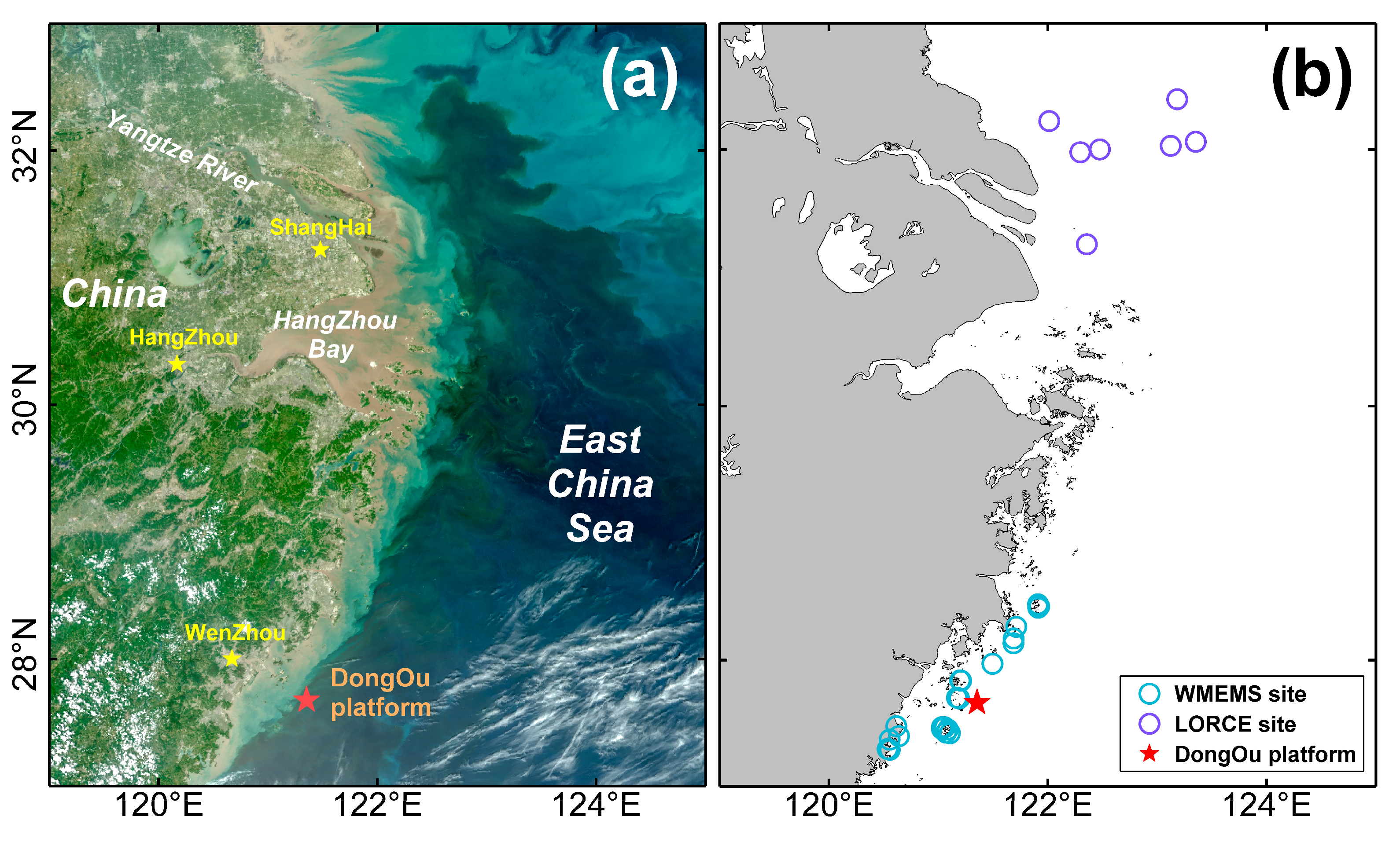
3.1. Assessment of Normalized Water-Leaving Radiance

Since the reliability of remote sensing monitoring of algal bloom mainly depends on the degree of the quantification of satellite derived R_rs, the R_rs at bands with lowest uncertainty and best degree of quantification in the study area should be preferred for constructing the algorithm. Validating the accuracy and spectral characteristics of VIIRS retrieved L_wn(λ) or the equivalent R_rs(λ) is, thus, an important prerequisite for carrying out algal bloom monitoring. A first step when evaluating the quality of the satellite data is to examine the spectral consistency of the water-leaving radiances from the VIIRS and MODIS missions based on the in situ data collected from the Dongou site. The Dongou site is frequently characterized by a large variability in bio-optical quantities because of its position in a transitional region between open sea and coastal waters (Figure 3a,e,i). Thus, the L_wn spectra from VIIRS and MODIS (Figure 3b,f,j) also show high variability. It can be found that the spectra exhibiting large variations show minima at 410 and 671 nm, with the majority of values below 20 W/m²/nm/sr and unique maxima at 551 nm with values in the range of 4.0–50 W/m²/nm/sr, and suggest the presence of seawater that is moderately dominated by sediments, as well as the derived water type provides a further confirmation with an occurrence of roughly 70% Case 2 water (of which MODISA, VIIRS-SNPP, and VIIRS-NA20 spectral data accounted for 75%, 83%, and 79% of this type, respectively) [42]. The comparison of L_wn spectra indicates that the spectral variation ranges of MODISA, VIIRS/SNPP, and VIIRS/NA20 are very consistent to each other. Furthermore, the matchup L_wn spectra from SeaPRISM was selected (Figure 3c,g,k); matchups of the overall average L_wn spectra were also calculated from all available spectral data of satellites and SeaPRISM, as seen in the fourth column of Figure 3d,h,l. These matchup comparisons indicate that a general spectral concordance exists between satellite and in situ data. However, in the average L_wn spectra match-up comparisons, a spectral discrepancy also can be observed at the shorter wavelength bands (410 and 443 nm).

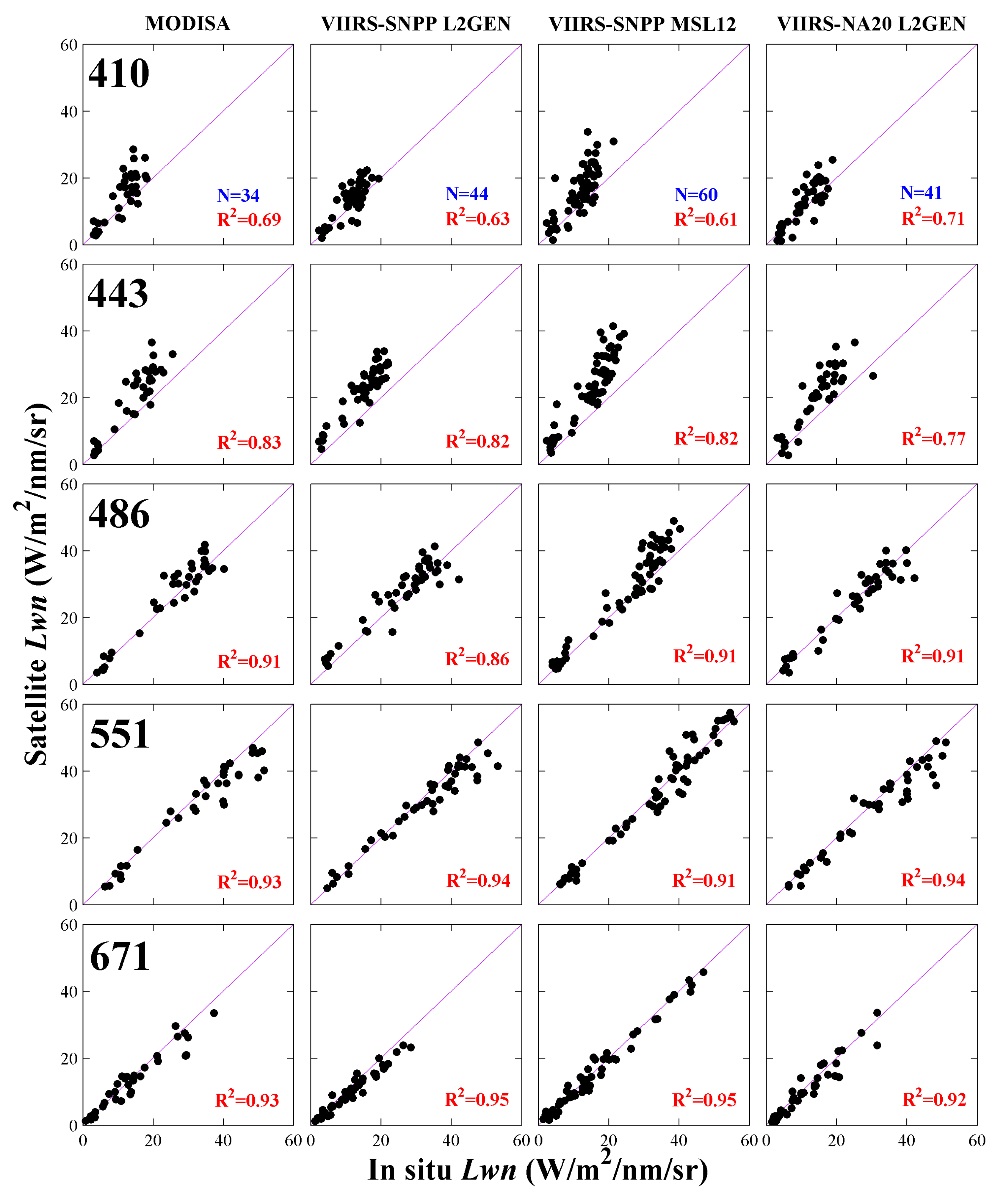
Thus, additional insight from the qualitative matchup analysis of satellite L_wn(λ) data against in situ SeaPRISM for each individual spectral band is presented in Figure 4 and

Table 4. Matchup statistics for four Satellite datasets according to QA_Wei check schemes. (Note: R², coefficients of correlation; RMSE, RAB, Ratio of Algal Bloom; APD, the average absolute percent differences; RPD, the average relative percent differences.).

Band (nm)	Parameter	MODISA	VIIRS-NPP L2GEN	VIIRS-NPP MSL12	VIIRS-N20 L2GEN
	N	34	44	60	41
410	R2	0.69	0.63	0.61	0.71
	RMSE	5.47	3.79	6.56	3.93
	APD (%)	37.35	28.14	50.24	29.67
	RPD (%)	29.75	18.92	9.22	7.23
443	R2	0.83	0.82	0.82	0.77
	RMSE	7.16	8.14	9.62	7.46
	APD (%)	39.48	61.55	59.89	48.88
	RPD (%)	38.31	61.09	59.86	43.29
486	R2	0.91	0.86	0.91	0.91
	RMSE	3.71	4.07	5.14	3.23
	APD (%)	13.17	17.73	16.50	11.79
	RPD (%)	5.41	12.45	13.25	0.27
551	R2	0.93	0.94	0.91	0.94
	RMSE	4.45	3.77	4.86	4.02
	APD (%)	9.91	8.81	8.01	9.58
	RPD (%)	−7.05	−2.44	−1.56	−6.35
671	R2	0.93	0.95	0.95	0.92
	RMSE	2.88	2.28	1.80	2.39
	APD (%)	17.17	16.67	17.10	16.91
	RPD (%)	−1.95	−10.75	2.64	−8.64

. After the quality control methods were applied, a total of 135 in situ L_wn spectra matched up with at least one satellite dataset, in which there are 34, 60, and 41 matchups available for MODIS/Aqua, VIIRS/SNPP MSL12, and VIIRS/NA20, respectively. It is noticeable that only 44 matchups were available for VIIRS-SNPP L2GEN, less than that for VIIRS- SNPP MSL12, because much tighter restrictions in the flag conditions applied in the filtering cloud and bright pixels were implemented in the L2GEN procedure. Additionally, the number of matchups of MODSA was less than the other three VIIRS sources, probably because the coastal water of the ECS is dominated by sediments (as seen in Figure 3a,e,i), which will more easily result in saturation of MODIS 862 nm and thus makes fewer matchups with L_wn spectra available.

Overall, the correlation coefficients (R²) between the SeaPRISM and satellite datasets at each wavelength were relatively high, and all comparisons, particularly at 488 nm, 551 nm, and 671 nm, were also very close to a 1:1 line (Figure 4). Notably, the MODISA data performed quite well even though this MODIS sensor has been in operation during orbit for more than 17 years and has long passed its expected lifetime. At individual wavelengths, correlations for the four satellites were very close to each other, which indicate good consistency between MODIS and the two VIIRS sensors; in addition, the variations in the water-leaving radiance data for the Dongou location were well captured by all satellite sensors. Nevertheless, the resulting R² values showed strong spectral dependencies exhibiting the tendency of displaying larger differences in the shorter end of the spectrum. For example, VIIRS-SNPP MSL12 achieved stronger R² values of 0.91, 0.91, and 0.95 at 486 nm, 551 nm, and 671 nm, respectively, while at 410 nm and 443 nm only moderate correlations were attained with R² values equal to 0.61 and 0.82, respectively. Similar spectral behavior and values of R² can be found in MODISA, VIIRS-SNPP L2GEN, and VIIRS-NA20 L2GEN comparisons. This degradation in the correlation for 410 nm and 443 nm agrees with more recent findings from the Long Island Sound coasts, USA, which was considered to have originated from the data processing procedure [10].

In addition, percent differences (APD and RPD) suggest good qualities of L_wn retrievals from satellites at 488 nm, 551 nm, and 671 nm, although high uncertainties and bias still exist at 410 nm and 443 nm (Table 4). The highest APD values were observed at 443 nm (with 39.48%, 61.55%, 59.89%, and 48.88% for MODISA, VIIRS-NPP L2GEN, VIIRS-NPP MSL12, and VIIRS-N20 L2GEN, respectively), followed by 410 nm with a minimum of 28.14%. The larger uncertainties further confirmed the moderate correlations at the two deep blue bands. In the individual band match-up comparisons (Figure 4), it can be found in all the four datasets that had satellite-derived L_wn at 410 nm and 443 nm as a whole were larger than that from SeaPRISM; a similar trend was shown in comparisons of the average L_wn spectra (Figure 3). Although these overestimates could be partially attributed to the uncertainties in the SeaPRISM datasets, limited retrieval accuracies were achieved at the two blue bands in both MODIS and VIIRS, indicating the challenge of using current remote sensing L_wn at 410 nm and 443 nm to derive bio-optical products for the ECS. Despite these problems, as compared to shorter wavelengths, matchup statistics were much better for the 486 nm, 551 nm, and 671 nm wavelengths.

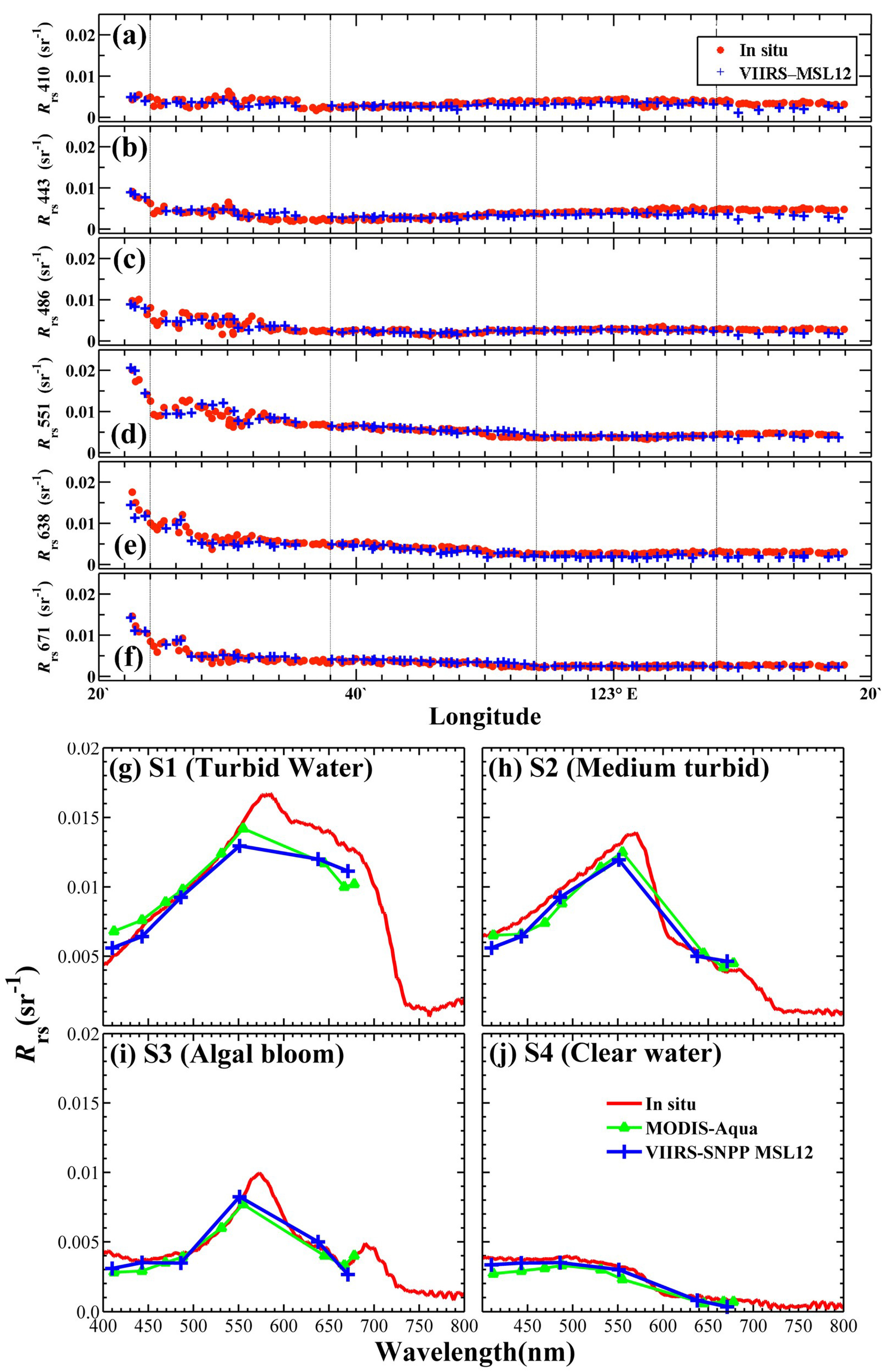
In order to fully access the VIIRS R_rs products, the supplementary underway R_rs measurements in the ECS were used. Figure 5 shows that the section of underway R_rs measurements crossed the coastal area from turbid to clean water bodies; it fortunately covered turbid, moderately turbid, clean, and HAB water bodies at the same time. Although it does not cover extremely turbid water bodies, the HAB events were very infrequent in such turbid waters due to light limitations; the satellite R_rs data were usually not available. Figure 5a–f shows the validation results of the section of underway R_rs observation against the VIIRS MSL12 R_rs data. Similar to the validation results at the Dongou platform (Figure 4), the VIIRS R_rs data of 410 nm and 443 nm showed a relatively high bias, while those at the 486 nm, 551 nm, and 671 nm bands were in very good agreement with the underway data. The spectral comparison in the four sites associated with turbid, moderately turbid, HAB, and clean water bodies is also presented in Figure 5g–j. In terms of magnitude and spectral shape, R_rs results obtained from VIIRS were very consistent with field measurements.

In the aggregate, these analyses show that as attributing to the most recent calibration efforts (and associated atmospheric correction routines) and reprocessing efforts of both NOAA and NASA, the MODISA, VIIRS/SNPP, and VIIRS/NA20 datasets from either NASA or NOAA yield reliable performance and consistent environmental data records, showing the band data of 486 nm, 551 nm, and 671 nm had better potential for the long-term monitoring in coasts of the ECS.

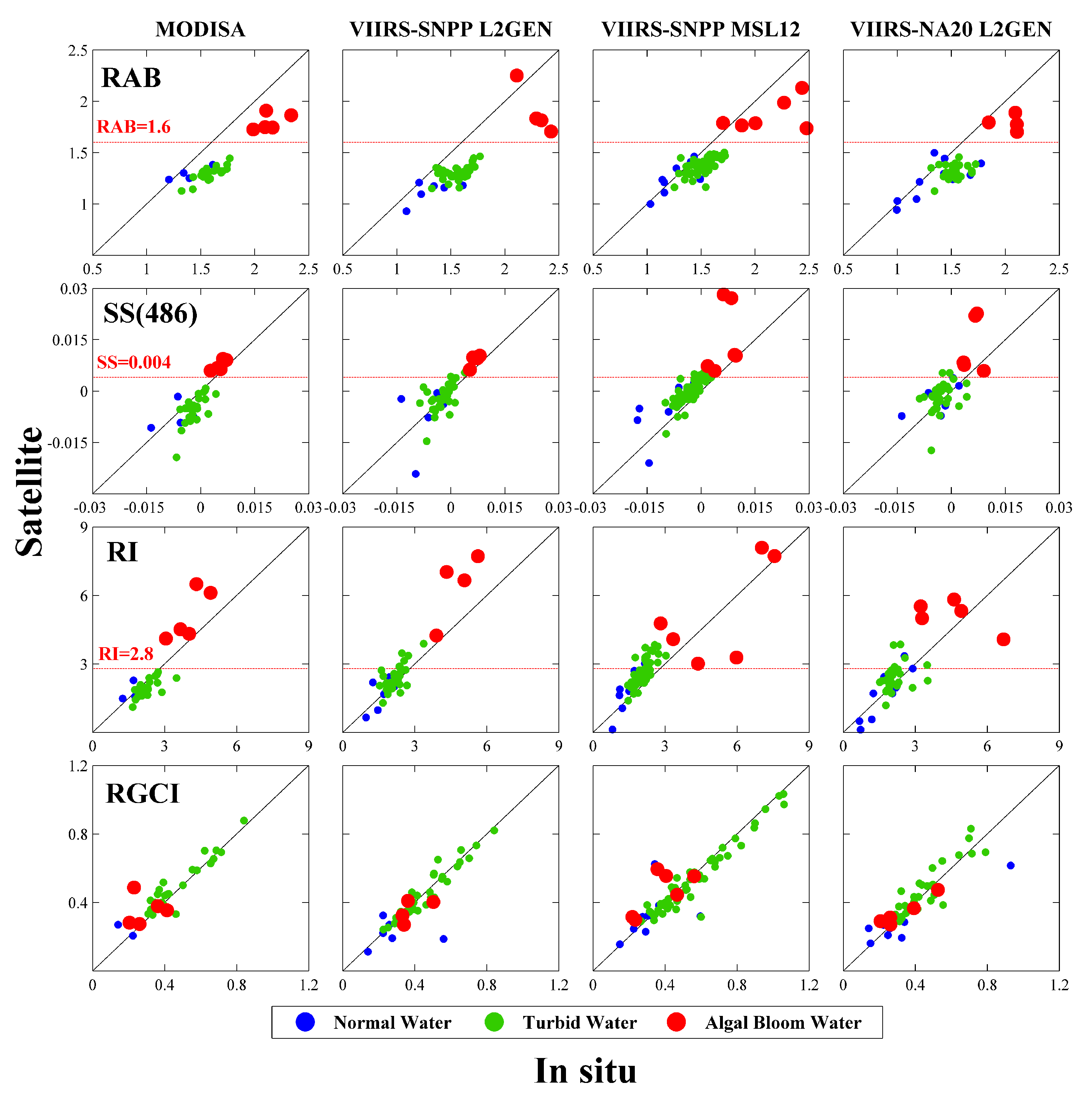
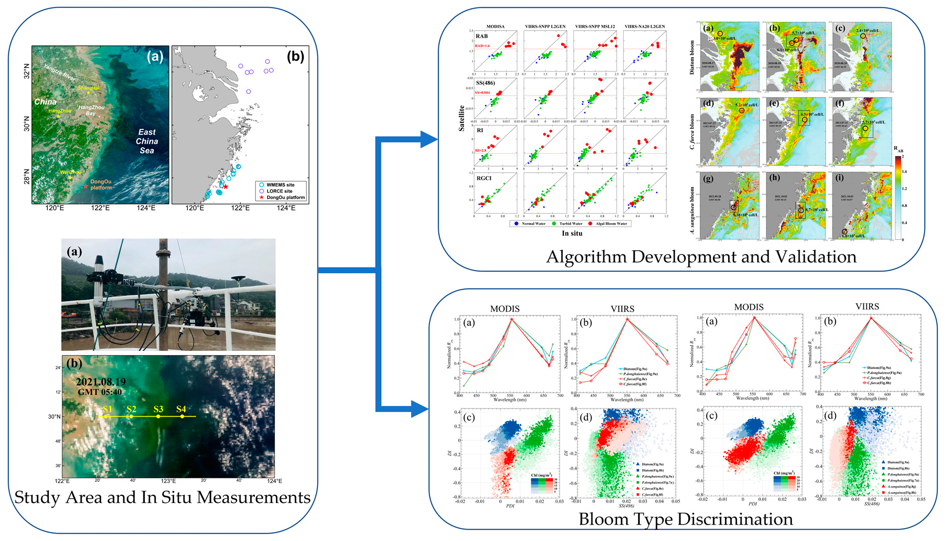
3.2. HAB Algorithm Development and Validation

Comparative analysis of various VIIRS algorithms was carried out to assess advantages and limitations in the application of these techniques for the detection of algal blooms in the sediment-dominated coasts of the ECS. Recently, different forms of HAB algorithms have become available, which specially include reflectance band-ratios and spectral band difference models [47]. As seen in Table 2, the two band-ratio algorithms, Algal Bloom Ratio (RAB) [28] and RGCI, and the two spectral band difference ones, Red Tide index (RI) [46] and normalized spectral shape at 488 nm (SS(488)), were selected for the comparison. Due to the similar band configuration of VIIRS with MODIS, most of these MODIS based algorithms can be directly applied to VIIRS. However, as mentioned above, VIIRS lacks the 531 nm band so that the 488 nm and 551 nm bands were used instead of MODIS 531 and 555 nm bands in the RAB algorithm.

Figure 6 shows scatterplots of in situ/satellite matchups for the four HAB indices, in which the algal bloom observations confirmed by field measurements at the Dongou site are plotted as red circles, as well as green circles indicating turbid waters with R_rs(551) greater than 0.014 sr⁻¹, and blue circles were associated with clear ones with R_rs(551) lower than 0.014 sr⁻¹. General consistency between satellite data and the SeaPRISM data can be found for all the four indices, but a difference exists in the capacity of the separation of bloom waters from normal ones. However, for sediment-dominated waters, the optical properties in the red bands were determined by both phytoplankton and sediment, and thus the separation of bloom areas from turbid waters by RGCI was not satisfactory. Although the performance of RI and SS(486) seems to be better, the separation in the two methods makes both not clear enough, probably because the blue band of 443 nm with relative high uncertainties was used in both of them. Thus, it can be clearly found that the RAB method probably yielded the best discrimination and the threshold value of 1.6 seems suitable for both MODIS and VIIRS for the identification of algal blooms. This success can be attributed not only to good quality of 488 nm and 551 nm data (Figure 4), but also to the much shearer slope between 488 nm and 551 nm of phytoplankton absorption [28].

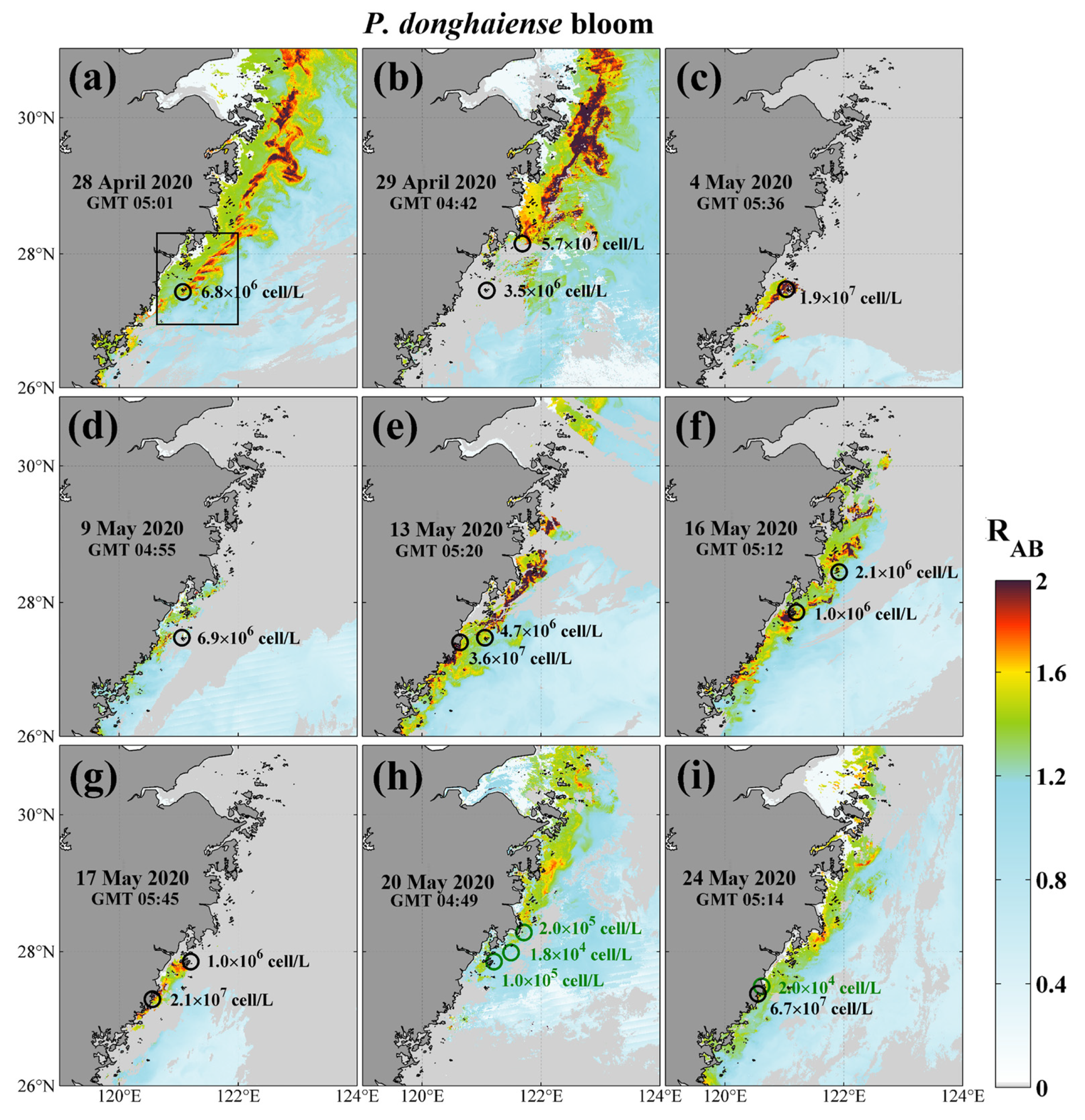
To further access the performance of the simple VIIRS RAB method in identifying HAB in the ECS, image series and near-concurrent field surveys for large-scale P. donghaiense blooms in April to May 2020 were used for method validation (Figure 7). These blooms were massive, extending over thousands of square kilometers, and persisted for nearly one month. The field measurements of cell counts from WMEMC confirmed that the RAB method can successfully differentiate bloom and non-bloom waters. 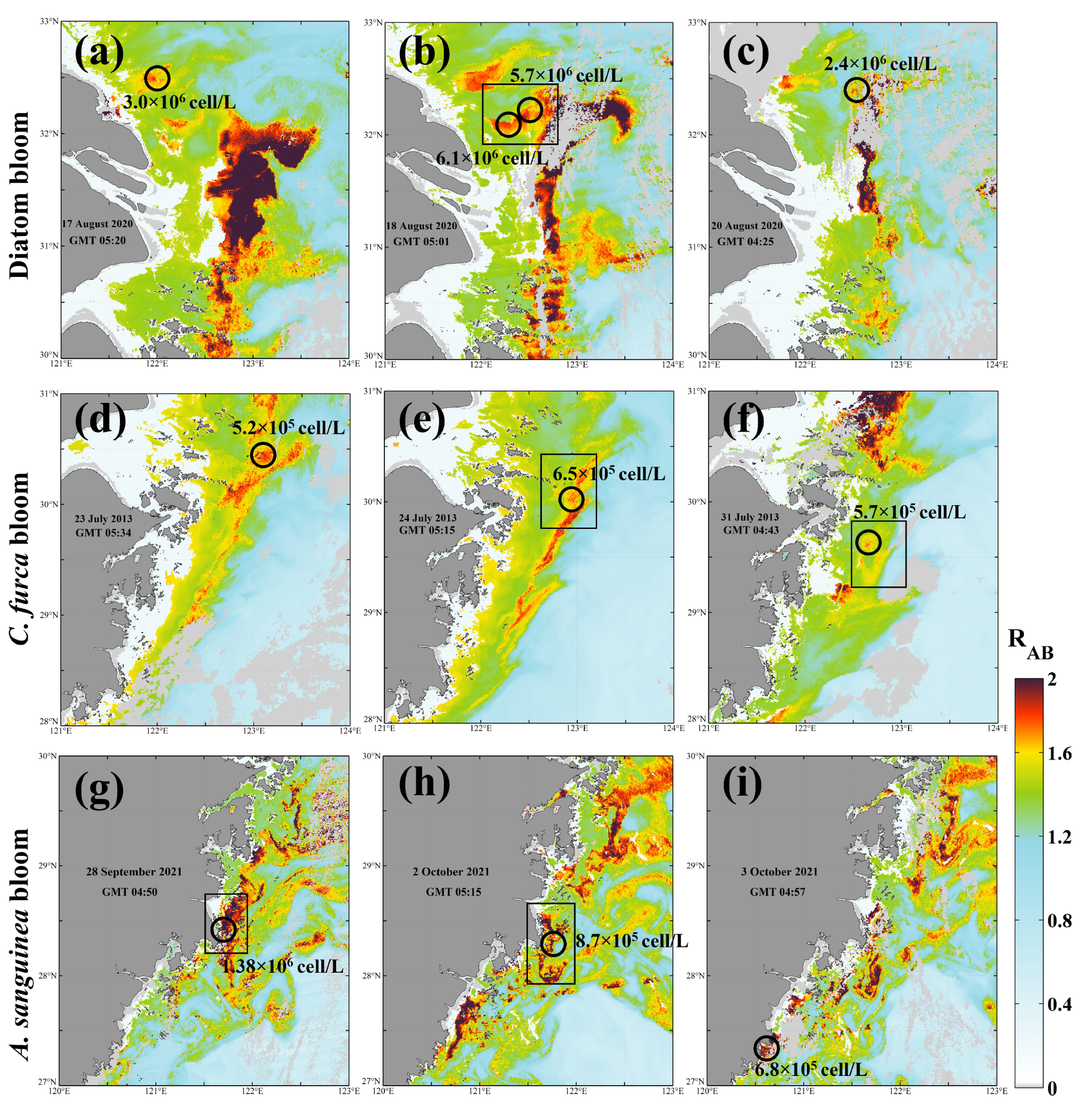Particularly, even in a very near-shore region, as seen in Figure 7e,f, small-area bloom events can also be captured in the RAB images. Similar success was achieved in the diatom bloom event occurring near the YRE in August 2020 (Figure 8a–c), indicating that RAB is also suitable for diatom bloom detection. In addition, RAB can also identify blooms dominated by other algal species, such as C. furca and A. sanguinea, validation results of which are shown in Figure 8d,e,g–i, respectively. Although there is an hourly error in the matchups of VIIRS derived RAB data and field surveys, these results are still sufficient to confirm the ability of VIIRS to detect HABs in the ECS.

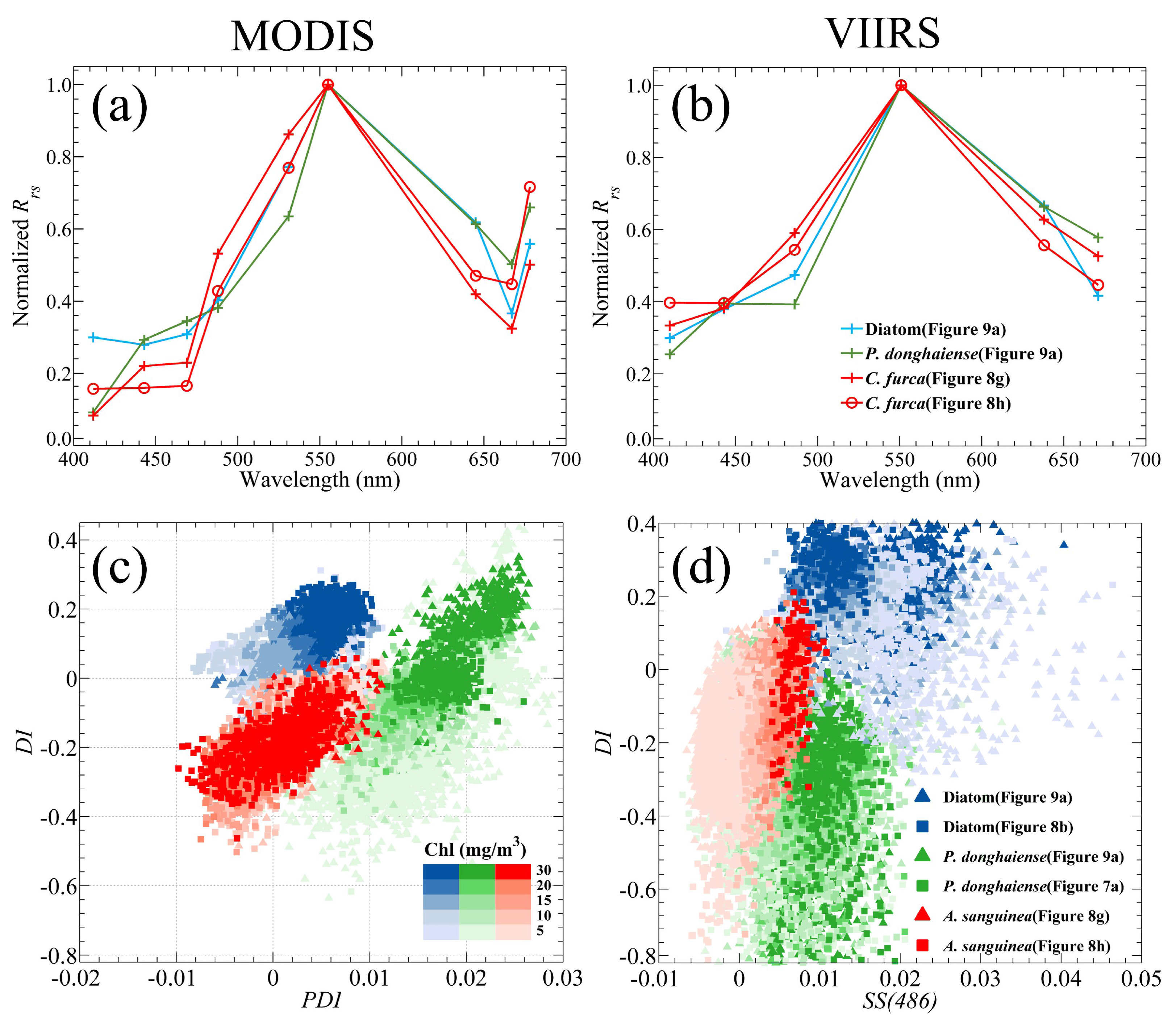
3.3. Capability in Bloom Type Discrimination

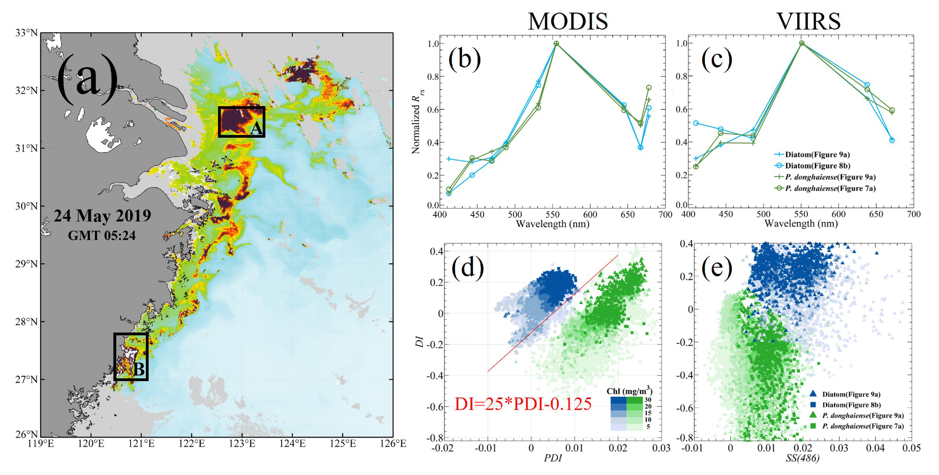
Although the reduction in the number of VIIRS bands has little impact on the identification of HABs in the ECS, it was found that it has a significant impact on the discrimination of bloom types or dominant species. Figure 9a shows the distribution of HAB events on 24 May 2019; note that the dominant algal species in region A was identified as P. donghaiense, while the one of region B in the other end of the stretch was caused by diatoms. In the above two regions, the typical R_rs spectra of P. donghaiense and diatom blooms from both MODIS and VIIRS were normalized by the maximum value of each spectrum in the green bands (Figure 9b,c). Other R_rs spectra of` P. donghaiense blooms that occurred on 28 April 2020 (Figure 7a) and a diatom bloom that occurred on 18 August 2020 (Figure 8b) are also presented. According to the finding of Tao et al. [28], the MODIS derived spectra of P. donghaiense and diatoms show a large difference mainly near the 531 nm and 645 nm bands; the R_rs of diatoms has a high shoulder peak at the 645 nm while that of P. donghaiense has a more obvious trough at 531 nm (Figure 9b). Therefore, the P. donghaiense bloom can be concluded as having extremely high PDI value and relatively low DI value compared to those of diatoms; then, the two type blooms can be clearly classified in the scatter plot of DI against PDI (Figure 9d). For VIIRS, due to a lack of a band near 531 nm, the difference between P. donghaiense and diatoms in their VIIRS R_rs spectra was only observed at 638 nm (Figure 9c). After the replacement of the PDI index by SS(486) for VIIRS, the separation of P. donghaiense and diatoms in the scatter plot of SS(486) against DI is not clear enough when compared with that in MODIS (Figure 9e). In contrast to PDI, SS(486) did not have obvious data that could be used to distinguish between P. donghaiense and diatoms; nevertheless, owing to the presence of the DI index, a clear trend still exists that can be used to separate the two types of blooms. Although VIIRS still has the ability to distinguish between P. donghaiense and diatoms in the ECS to some extent, the lack of a 531 nm band greatly reduces its ability to discriminate other types of algal blooms.

Based on the observation of the C. furca blooms in July 2013, its R_rs spectra derived from MODIS showed some distinguishing spectral features that can be used to separate them from P. donghaiense and diatom blooms (Figure 10a). Compared with diatoms, a C. furca bloom does not have a prominent shoulder peak at 645 nm, while compared with P. donghaiense, it has no reflection trough at 531 nm. These features can be directly reflected in the scatter plot of PDI to DI (Figure 10c). The clusters of C. furca blooms are roughly located in the lower left quarter of Figure 10c so that the separation between C. furca and diatom blooms is very clear, although some points of a C. furca bloom are not well separated from clusters associated with P. donghaiense. Nevertheless, the classification of C. furca, P. donghaiense, and diatom blooms cannot be achieved based on the VIIRS data, since the VIIRS derived R_rs spectra between 488 nm and 551 nm of a C. furca bloom do not yield different features from the other two types of blooms when the 531 nm band is not available (Figure 10b,d).

For A. sanguinea blooms, there is another interesting feature found near 488 nm in R_rs spectra of both MODIS and VIIRS (Figure 11a,b), which makes both PDI and SS(486) of A. sanguinea become significantly lower than that of P. donghaiense. Similar to the classification results of C. furca, the distribution of A. sanguinea points in the PDI-DI scatter plot of MODIS (Figure 11c) is at the lower left of P. donghaiense and diatom clusters, and more importantly, the distinction between the A. sanguinea and other two type blooms is more evident. Comparatively, the distribution of A. sanguinea points in the SS(486)-DI scatter plot of VIIRS partially overlaps with the P. donghaiense and diatom points (Figure 11d), but the separations of A. sanguinea from the P. donghaiense and diatom blooms is also better than that of C. furca (Figure 10d). Although the classification results of VIIRS showed a certain trend of separation, but was still not enough to separate A. sanguinea from P. donghaiense and diatoms. Based on the above results, one can conclude that the 531 nm band is essential for the bloom type discrimination, a lack of which significantly limits the capability of VIIRS.

4. Conclusions

This paper involved a systematic assessment of VIIRS for its ability to detect HAB and classify bloom types in coastal waters of the ECS. Although the data in the 412 and 443 nm bands had relatively high uncertainties, we found that the data quality at the 486, 551, and 671 nm was reliable. The above three bands show strong stability and consistency in the comparison of data accuracy and spectral characteristics of VIIRS. More importantly, we determined the accuracy of VIIRS data in different water bodies through a comparison with R_rs data collected during LORCE underway observation, which showed that the three bands were fully competent for construction of the algorithm for long-term HAB monitoring due to their high data quality. The applicability of different HAB algorithms in the ECS also varied. The two spectral shape algorithms, RI and SS(486), were less effective because they used the 443 nm with poor stability, and because of the red light absorption characteristics of suspended sediment, RGCI was not suitable for the detection of HABs in sediment-rich coasts of the ECS. Only RAB, thanks to the high quality of 486 nm, 551 nm, and the shearer slope of the two bands, has the best recognition effect and can accurately identify different types of algae. It is noteworthy that, due to the absence of the band near 531 nm, VIIRS was able to separate P. donghaiense from diatoms, but the ability to discriminate a third type of algae was significantly limited more than that of MODIS. We could hardly discriminate C. furca or A. sanguinea from P. donghaiense and diatoms using VIIRS data, and although A. sanguinea showed some separation trend, the effect was still insufficient to distinguish them. Therefore, it is suggested that subsequent ocean color satellite sensors should be set in a band near 531 nm, which will be of great benefit to the detection and classification of different types of algal bloom.

References

1. Butler, J.J.; Xiong, X.; Barnes, R.A.; Patt, F.S.; Chiang, K. An overview of Suomi NPP VIIRS calibration maneuvers. SPIE Opt. Eng. Appl. 2012, 8510, 603–615. [Google Scholar]
2. Xiong, X.; Butler, J.; Chiang, K.; Efremova, B.; Fulbright, J.; Lei, N.; McIntire, J.; Oudrari, H.; Sun, J.; Wang, Z.; et al. VIIRS on-orbit calibration methodology and performance. J. Geophys. Res. D Atmos. JGR 2014, 119, 5065–5078. [Google Scholar] [CrossRef]
3. Ardanuy, P.E.; Schueler, C.; Miller, S.W.; Jensen, K.; Emery, W.J. Use of CAIV techniques to build advanced VIIRS approaches for NPOESS key EDRs. Proc. SPIE 2002, 4814, 142–151. [Google Scholar]
4. Wang, M.; Liu, X.; Tan, L.; Jiang, L.; Tan, L.; Son, S.; Shi, W. Impacts of VIIRS SDR performance on ocean color products. J. Geophys. Res. D Atmos. JGR 2013, 118, 10347–10360. [Google Scholar] [CrossRef]
5. Lin, Q.; Hu, C.; Cannizzaro, J.; Corcoran, A.; English, D.; Le, C. VIIRS Observations of a Karenia brevis Bloom in the Northeastern Gulf of Mexico in the Absence of a Fluorescence Band. IEEE Geosci. Remote Sens. Lett. 2015, 12, 2213–2217. [Google Scholar]
6. Wang, M.; Jiang, L. VIIRS-derived ocean color product using the imaging bands. Remote Sens. Environ. 2018, 206, 275–286. [Google Scholar] [CrossRef] [Green Version]
7. Jiang, G.; Loiselle, S.A.; Yang, D.; Ma, R.; Gao, C. Remote estimation of chlorophyll a concentrations over a wide range of optical conditions based on water classification from VIIRS observations. Remote Sens. Environ. 2020, 241, 111735. [Google Scholar] [CrossRef]
8. Wang, C.; Wang, M.; Chen, B.; Qin, W.; Lin, L.; Dai, C.; Hengguo, Y.U.; Renhui, L.I.; Zhao, M.; Zengling, M.A. Harmful algal bloom-forming dinoflagellate Prorocentrum donghaiense inhibits the growth and photosynthesis of seaweed Sargassum fusiformis embryos. J. Mar. Limnol. 2021, 39, 15. [Google Scholar] [CrossRef]
9. Hu, C.; Barnes, B.B. Dependence of satellite ocean color data products on viewing angles: A comparison between SeaWiFS, MODIS, and VIIRS. Remote Sens. Environ. Interdiscip. J. 2016, 175, 120–129. [Google Scholar]
10. Hlaing, S.; Harmel, T.; Gilerson, A.; Foster, R.; Weidemann, A.; Arnone, R.; Wang, M.; Ahmed, S. Evaluation of the VIIRS ocean color monitoring performance in coastal regions. Remote Sens. Environ. 2013, 139, 398–414. [Google Scholar] [CrossRef]
11. Barnes, B.; Cannizzaro, J.P.; English, D.C.; Hu, C. Validation of VIIRS and MODIS reflectance data in coastal and oceanic waters: An assessment of methods. Remote Sens. Environ. 2019, 220, 110–123. [Google Scholar] [CrossRef] [Green Version]
12. Schofield, O.; Grzymski, J.; Bissett, W.P.; Kirkpatrick, G.J.; Millie, D.; Moline, M.; Roesler, C.S. Optical monitoring and forecasting systems for harmful algal blooms: Possibility or pipe dream? J. Phycol. 1999, 35, 1477–1496. [Google Scholar] [CrossRef] [Green Version]
13. Stumpf, R.P.; Culver, M.E.; Tester, P.A.; Tomlinson, M.C.; Soracco, M. Monitoring Karenia Brevis Blooms in the Gulf of Mexico Using Satellite Ocean Color Imagery and Other Data. Harmful Algae 2003, 2, 147–160. [Google Scholar] [CrossRef]
14. Stumpf, R.P.; Tomlinson, M.C. Use of remote sensing in monitoring and forecasting of harmful algal blooms. Proc. SPIE Int. Soc. Opt. Eng. 2004, 5885, 58850I. [Google Scholar]
15. Cannizzaro, J.P.; Carder, K.L.; Chen, F.R.; Heil, C.A.; Vargo, G.A. A novel technique for detection of the toxic dinoflagellate, Karenia brevis, in the Gulf of Mexico from remotely sensed ocean color data. Cont. Shelf. Res. 2008, 28, 137–158. [Google Scholar] [CrossRef]
16. Carvalho, G.A.; Minnett, P.J.; Fleming, L.E.; Banzon, V.F.; Baringer, W. Satellite remote sensing of harmful algal blooms: A new multi-algorithm method for detecting the Florida Red Tide (Karenia brevis). Harmful Algae 2010, 9, 440–448. [Google Scholar] [CrossRef] [Green Version]
17. Hu, C.; Muller-Karger, F.E.; Taylor, C.; Carder, K.L.; Kelble, C.; Johns, E.; Heil, C.A. Red tide detection and tracing using MODIS fluorescence data: A regional example in SW Florida coastal waters. Remote Sens. Environ. 2005, 97, 311–321. [Google Scholar] [CrossRef]
18. Carder, K.L.; Chen, F.R.; Cannizzaro, J.P.; Campbell, J.W.; Mitchell, B.G. Performance of the MODIS semi-analytical ocean color algorithm for chlorophyll-a. Adv. Space Res. 2004, 33, 1152–1159. [Google Scholar] [CrossRef]
19. Cannizzaro, J.P.; Barnes, B.B.; Hu, C.; Corcoran, A.A.; Kelble, C.R. Remote detection of cyanobacteria blooms in an optically shallow subtropical lagoonal estuary using MODIS data. Remote Sens. Environ. 2019, 231, 111227. [Google Scholar] [CrossRef]
20. Zibordi, G.; Berthon, J.F.; Mélin, F.; D’Alimonte, D.; Kaitala, S. Validation of satellite ocean color primary products at optically complex coastal sites: Northern Adriatic Sea, Northern Baltic Proper and Gulf of Finland. Remote Sens. Environ. 2009, 113, 2574–2591. [Google Scholar] [CrossRef]
21. Hu, C.; Barnes, B.; Qi, L.; Corcoran, A. A Harmful Algal Bloom of Karenia brevis in the Northeastern Gulf of Mexico as Revealed by MODIS and VIIRS: A Comparison. Sensors 2015, 15, 2873–2887. [Google Scholar] [CrossRef] [PubMed] [Green Version]
22. Ahn, Y.H.; Shanmugam, P. Detecting the red tide algal blooms from satellite ocean color observations in optically complex Northeast-Asia Coastal waters. Remote Sens. Environ. 2006, 103, 419–437. [Google Scholar] [CrossRef]
23. Hu, C.; Lee, Z.; Ma, R.; Yu, K.; Li, D.; Shang, S. Moderate Resolution Imaging Spectroradiometer (MODIS) observations of cyanobacteria blooms in Taihu Lake, China. J. Geophys. Res. 2010, 115. [Google Scholar] [CrossRef] [Green Version]
24. Siswanto, E.; Ishizaka, J.; Tripathy, S.C.; Miyamura, K. Detection of harmful algal blooms of Karenia mikimotoi using MODIS measurements: A case study of Seto-Inland Sea, Japan. Remote Sens. Environ. 2013, 129, 185–196. [Google Scholar] [CrossRef]
25. Feng, C.; Ishizaka, J.; Saitoh, K.; Mine, T.; Yamashita, H. A Novel Method Based on Backscattering for Discriminating Summer Blooms of the Raphidophyte (Chattonella spp.) and the Diatom (Skeletonema spp.) using MODIS Images in Ariake Sea, Japan. Remote Sens. 2020, 12, 1504. [Google Scholar] [CrossRef]
26. Kim, Y.; Lee, K.D.; Na, S.I.; Hong, S.Y.; Yoo, H.Y. MODIS Data-based Crop Classification using Selective Hierarchical Classification. Korean J. Remote Sens. 2016, 32, 235–244. [Google Scholar] [CrossRef]
27. Shang, S.; Wu, J.; Huang, B.; Lin, G.; Lee, Z.; Liu, J.; Shang, S. A new approach to discriminate dinoflagellate from diatom blooms from space in the East China Sea. J. Geophys. Res. Oceans 2015, 119, 4653–4668. [Google Scholar] [CrossRef]
28. Tao, B.; Mao, Z.; Lei, H.; Pan, D.; Shen, Y.; Bai, Y.; Zhu, Q.; Li, Z. A novel method for discriminating Prorocentrum donghaiense from diatom blooms in the East China Sea using MODIS measurements. Remote Sens. Environ. 2015, 158, 267–280. [Google Scholar] [CrossRef]
29. Sun, W.; Xie, Z.; Chen, J.; Zhang, X.; Chai, Z.; Du, A.; Zhao, J.; Zhang, C.; Zhou, T. Os-Os dating of copper and molybdenum deposits along the middle and lower reaches of the Yangtze River, China. Econ. Geol. 2003, 98, 175–180. [Google Scholar] [CrossRef]
30. Wang, Z.; Li, L.; Chen, D.; Xu, K.; Wei, T.; Gao, J.; Zhao, Y.; Chen, Z.; Masabate, W. Plume front and suspended sediment dispersal off the Yangtze (Changjiang) River mouth, China during non-flood season. Estuar. Coast. Shelf. Sci. 2007, 71, 60–67. [Google Scholar] [CrossRef]
31. Jiang, Z.; Gao, Y.; Zhai, H.; Jin, H.; Zhou, F.; Shou, L.; Yan, X.; Chen, Q. Regulation of spatial changes in phytoplankton community by water column stability and nutrients in the southern Yellow Sea. J. Geophys. Res. Biogeosci. 2019, 124, 2610–2627. [Google Scholar] [CrossRef]
32. Chen, Y.; Xu, Q.; Gibson, K.; Chen, N. Metabarcoding dissection of harmful algal bloom species in the East China Sea off Southern Zhejiang Province in late spring. Mar. Pollut. Bull. 2021, 169, 112586. [Google Scholar] [CrossRef] [PubMed]
33. GB 17378.7–2007; Marine Monitoring Specification Seventh Part: Coastal Pollution Ecological Investigation and Biological Monitoring. China Standards Press: Beijing, China, 2007.
34. Zibordi, G.; Mélin, F.; Berthon, J.F.O.; Holben, B.; Slutsker, I.; Giles, D.; D’Alimonte, D.; Vandemark, D.; Feng, H.; Schuster, G. AERONET-OC: A Network for the Validation of Ocean Color Primary Products. J. Atmos. Ocean Technol. 2009, 26, 1634–1651. [Google Scholar] [CrossRef]
35. Clark, D.K.; Yarbrough, M.A.; Feinholz, M.; Flora, S.; Broenkow, W.; Kim, Y.S.; Johnson, B.C.; Brown, S.W.; Yuen, M.; Mueller, J.L. MOBY, A radiometric buoy for performance monitoring and vicarious calibration of satellite ocean color sensors: Measurement and data analysis protocols. In Ocean Optics Protocols for Satellite Ocean Color Sensor Validation; National Aeronautics and Space Administration: Washington, DC, USA, 2003; pp. 1–34. [Google Scholar]
36. Wang, M.; Gordon, H.R. A simple, moderately accurate, atmospheric correction algorithm for SeaWiFS. Remote Sens. Environ. 1994, 50, 231–239. [Google Scholar] [CrossRef]
37. Stumpf, R.P.; Arnone, R.A.; Gould, R.W.; Martinolich, P.M.; Ransibrahmanakul, V. A partially coupled ocean-atmosphere model for retrieval of water-leaving radiance from SeaWiFS in coastal waters. NASA Tech. Memo 2003, 206892, 51–59. [Google Scholar]
38. Werdell, P.J.; Franz, B.A.; Bailey, S.W. Evaluation of shortwave infrared atmospheric correction for ocean color remote sensing of Chesapeake Bay. Remote Sens. Environ. 2010, 114, 2238–2247. [Google Scholar] [CrossRef] [Green Version]
39. Mobley, C.D.; Werdell, J.; Franz, B.; Ahmad, Z.; Bailey, S. Atmospheric Correction for Satellite Ocean Color Radiometry; National Aeronautics and Space Administration: Washington, DC, USA, 2016; pp. 13–29.
40. Wang, M.; Wei, S. The NIR-SWIR combined atmospheric correction approach for MODIS ocean color data processing. Opt. Express 2007, 15, 15722–15733. [Google Scholar] [CrossRef] [PubMed] [Green Version]
41. Jiang, L.; Wang, M. Improved near-infrared ocean reflectance correction algorithm for satellite ocean color data processing. Opt. Express 2014, 22, 21657–21678. [Google Scholar] [CrossRef] [PubMed]
42. Wei, J.; Lee, Z.; Shang, S. A system to measure the data quality of spectral remote-sensing reflectance of aquatic environments. J. Geophys. Res. C Oceans JGR 2016, 121, 8189–8207. [Google Scholar] [CrossRef]
43. Schmutz, W.; Fehlmann, A.; Finsterle, W.; Kopp, G.; Thuillier, G. Total solar irradiance measurements with Premos/picard. AIP Conf. Proc. 2013, 1531, 624–627. [Google Scholar]
44. Shanmugam, P.; Kim, H.-C.; Ahn, Y.H.; Moon, J.E.; Tiwari, S.P. An Evaluation Of Modis/Aqua Bio-Optical Algorithms In Arctic Waters. Environ. Eng. Manag. J. 2013, 12, 2219–2232. [Google Scholar]
45. Zibordi, G.; Mélin, F.; Hooker, S.B.; D’Alimonte, D.; Holben, B. An autonomous above-water system for the validation of ocean color radiance data. IEEE Trans. Geoence Remote Sens. 2004, 42, 401–415. [Google Scholar] [CrossRef]
46. Lou, X.; Hu, C. Diurnal changes of a harmful algal bloom in the East China Sea: Observations from GOCI. Remote Sens. Environ. 2014, 140, 562–572. [Google Scholar] [CrossRef]
47. Tilstone, G.H.; Taylor, B.H.; Blondeau-Patissier, D.; Powell, T.; Lucas, M.I. Comparison of new and primary production models using SeaWiFS data in contrasting hydrographic zones of the northern North Atlantic. Remote Sens. Environ. 2014, 156, 473–489. [Google Scholar] [CrossRef] [Green Version]
Figure 1. (a) Visible Infrared Imaging Radiometer Suite false color composed image of the East China Sea (ECS) collected on 28 April 2020 (R: 671 nm, G: 551 nm, B: 486 nm). Most regions in the ECS are covered by optically complex turbid or medium turbid waters that are rich in sediment along the coast. The star symbol shows the location of the Dongou oceanographic (Dongou) platform. (b) Map of sample locations from independent field datasets: Light blue circles and purple triangles show data collected by the Wenzhou Marine Environmental Monitoring Center Station (WMEMC) from April to May 2020 and data collected from the Long-term Observation and Research Plan in the Changjiang Estuary and Adjacent East China Sea (LORCE) cruise during the August 2020, respectively. A picture of the Dongou platform as an inset photo.
Remotesensing 14 02089 g001
Figure 2. (a) Photo of the CrusieAOP-T system. (b) Schematic diagram of the Long-term Observation and Research Plan in the Changjiang Estuary and Adjacent East China Sea underway observation section in 19 August 2021; the yellow line on the map is the track. The four stations numbered S1–S4 were selected to represent turbid water, medium turbid water, algal bloom water, and clear water, respectively.
Remotesensing 14 02089 g002
Figure 3. (a,e,i) A 2020 spring composite (March–May) of satellite-derived Lwn (551) maps for the coastal area in the East China Sea (the cross symbol indicates the location of the Dongou platform). (b,f,j) SeaPRISM in situ and (c,g,k) satellite Lwn Spectrum, whose colors represent the different water types defined by the QA_Wei method. (d,h,l) Mean Lwn spectrum, where red and blue lines represent in situ and satellite spectra, respectively.
Remotesensing 14 02089 g003
Figure 4. Scatterplots showing in situ/satellite remote sensing reflectance (Rrs; sr−1) matchups (black dots) after a QA_Wei check. Data are shown separately for MODISA (first column), VIIRS-NPP L2GEN (second column), VIIRS-NPP MSL12 (third column), and VIIRS-NA20 L2GEN (fourth column) and by waveband (from top row: 410 nm, 443 nm, 486 nm, 551 nm, and 671 nm). Note that the coefficient of determination (R2) for each QA checked matchup dataset is displayed in the lower right corner of each subplot.
Remotesensing 14 02089 g004
Figure 5. (af) Rrs comparison between the Long-term Observation and Research Plan in the Changjiang Estuary and Adjacent East China Sea underway observation section and VIIRS-SNPP MSL12, where the positions of S1–S4 are marked by dashed lines. (gj) Spectra of S1–S4, which represent turbid water, medium turbid water, algal bloom water, and clear water, respectively.
Remotesensing 14 02089 g005
Figure 6. Scatterplots showing in situ/satellite matchups for four harmful algal bloom indices. Data shown separately for RAB, SS(486), RI, and RGCI (from top to bottom) and for MODISA, VIIRS-SNPP L2GEN, VIIRS-SNPP MSL12, and VIIRS-NA20 L2GEN (from left to right).
Remotesensing 14 02089 g006
Figure 7. (ai) VIIRS-SNPP (MSL12) derived algal bloom ratio images from late April to May 2020 and their specific site images are shown in Figure A1 in the Appendix A. In the algal bloom ratio images, only the areas positively flagged as bloom waters are shown in yellow and red. The black and green circles indicate bloom and non-bloom sites (5 × 10⁵ cells/L is taken as the reference concentration of HAB [33]), which have been confirmed by field surveys; the cell count data are plotted close to the circle in each image. (Satellite data from the square area on the map were used for the subsequent classification of algal bloom types.).
Remotesensing 14 02089 g007
Figure 8. VIIRS/SNPP derived algal bloom ratio images in mid-August 2020, late July 2013, and late September to early October 2021, which are dominated by (ac) diatoms, (df) C. furca, and (gi) A. sanguinea, respectively. (Satellite data from the rectangular areas on the maps were used for subsequent classification of algal bloom types.) The specific site images of diatom and A. sanguinea blooms are shown in Figure A2 and Figure A3 in the Appendix A, respectively.
Remotesensing 14 02089 g008
Figure 9. (a) VIIRS/SNPP-MSL12 derived RAB image acquired on 24 May 2019, where the dominated algal species in regions A and B are P. donghaiense and diatoms, respectively. (b,c) Normalized Rrs spectra associated with P. donghaiense or diatoms, from MODIS and VIIRS, respectively. (d,e) Scatter plot of DI against PDI or SS(486) derived from MODIS and VIIRS data. The solid red line in (d) represents a line (expressed as DI = 25·PDI − 0.125 to separate P. donghaiense blooms from diatom blooms [28]. Satellite (MODIS and VIIRS) data of two P. donghaiense blooms were taken from A region of Figure 9a on 24 May 2019 and the rectangle region of Figure 7a on 28 April 2020, respectively, and data for the two diatom bloom events were taken from B region of Figure 9a on 24 May 2019 and the rectangle region of Figure 8b on 18 August 2020, respectively.
Remotesensing 14 02089 g009
Figure 10. (a,b) Normalized Rrs spectra of C. furca, P. donghaiense, and diatom blooms from MODIS and VIIRS, respectively. (c,d) Scatter plot of DI against PDI/SS(486) derived from MODIS/VIIRS data. The satellite data for P. donghaiense and diatoms are the same as those in Figure 9, while the data of C. furca are taken from the rectangle regions in Figure 8e,f on 24 and 31 July 2013, respectively.
Remotesensing 14 02089 g010
Figure 11. (a,b) Normalized spectra of MODIS and VIIRS derived Rrs(λ) associated with P. donghaiense, diatoms, and A. sanguinea, respectively. (c,d) Scatter plot of DI against PDI or SS(486) derived from MODIS or VIIRS data, respectively. The satellite data of P. donghaiense and diatom are the same as Figure 9, while the data of A. sanguinea are taken from the rectangle regions of Figure 8g,h on 28 September 2021 and 2 October 2021, respectively.
Remotesensing 14 02089 g011