Unsupervised Building Extraction from Multimodal Aerial Data Based on Accurate Vegetation Removal and Image Feature Consistency Constraint

Abstract

Accurate building extraction from remotely sensed data is difficult to perform automatically because of the complex environments and the complex shapes, colours and textures of buildings. Supervised deep-learning-based methods offer a possible solution to solve this problem. However, these methods generally require many high-quality, manually labelled samples to obtain satisfactory test results, and their production is time and labour intensive. For multimodal data with sufficient information, extracting buildings accurately in as unsupervised a manner as possible. Combining remote sensing images and LiDAR point clouds for unsupervised building extraction is not a new idea, but existing methods often experience two problems: (1) the accuracy of vegetation detection is often not high, which leads to limited building extraction accuracy, and (2) they lack a proper mechanism to further refine the building masks. We propose two methods to address these problems, combining aerial images and aerial LiDAR point clouds. First, we improve two recently developed vegetation detection methods to generate accurate initial building masks. We then refine the building masks based on the image feature consistency constraint, which can replace inaccurate LiDAR-derived boundaries with accurate image-based boundaries, remove the remaining vegetation points and recover some missing building points. Our methods do not require manual parameter tuning or manual data labelling, but still exhibit a competitive performance compared to 29 methods: our methods exhibit accuracies higher than or comparable to 19 state-of-the-art methods (including 8 deep-learning-based methods and 11 unsupervised methods, and 9 of them combine remote sensing images and 3D data), and outperform the top 10 methods (4 of them combine remote sensing images and LiDAR data) evaluated using all three test areas of the Vaihingen dataset on the official website of the ISPRS Test Project on Urban Classification and 3D Building Reconstruction in average area quality. These comparative results verify that our unsupervised methods combining multisource data are very effective.

1. Introduction

Building rooftop extraction plays a significant role in assessing the deployment space of photovoltaic facilities [1], estimating building energy consumption and emissions [2], urban management [3], disaster management [4,5,6,7], population estimation [8], three-dimensional reconstruction [9,10,11,12] and many other applications. However, to date, achieving automatic and accurate building extraction from remotely sensed data remains an unsolved problem in computer vision and remote sensing. In general, the number of buildings to be extracted is large; therefore, if they can be automatically and accurately extracted from remotely sensed data, a significant amount of labour can be saved. Otherwise, many human interventions, i.e., burdensome parameter tuning or manual annotation, are required. Theoretically, the efficiency of automatic methods can be significantly improved if the machines running them have been greatly upgraded, and the machines are indeed greatly upgraded periodically. However, the efficiency of semi-automatic methods cannot be improved in the same way because the reaction speed and the work intensity that human beings can bear are both very limited, and the situation will always be the same unless human bodies are greatly strengthened by some means. Furthermore, the cost of manual labour will increase with the development of society. Therefore, reducing the manual labour in building extraction is necessary, which, of course, also applies to other data-processing tasks.

Supervised deep-learning-based methods are a possible solution to realise automatic and accurate building extraction from remotely sensed data. The rapid development of deep learning, especially convolutional neural networks [13,14,15,16,17,18,19,20,21] and transformers [22,23,24], has made deep-learning-based methods the mainstream for building extraction, and many impressive results have been achieved. However, deep-learning-based methods still rely on a large number of labelled samples to obtain satisfactory results, and these samples are often manually labelled, which is time and labour consuming. Furthermore, if the test dataset and the training dataset differ greatly, the deep learning models may perform poorly [25,26,27], and new samples are often manually labelled to overcome this problem. Ideally, we would establish a very large dataset to cover as many types of buildings as possible, like the famous ImageNet dataset [28] for image classification tasks. However, such a practice is expensive to execute. To alleviate the manual data-labelling problem, some researchers proposed using semi-supervised methods [29], whereas some researchers proposed studying unsupervised methods [30]. This paper follows the latter kind because the automation level of this kind of methods is higher.

If we can extract sufficient information about the buildings from the used data in an unsupervised manner, it is possible to design an unsupervised method to extract buildings automatically and accurately, avoiding manual data labelling and manual parameter(s) tuning. According to the data types used, existing building extraction methods can be divided into three categories: (1) methods based on remote sensing images [20,31,32,33,34], (2) methods based on three-dimensional data (often LiDAR point clouds) [10,35,36,37,38,39], and (3) methods that combine remote sensing images and three-dimensional data [6,16,30,40,41,42,43].

Remote sensing images contain the spectral features and texture features of buildings, and implicitly contain geometric features. Geometric features are critical for building extraction, but existing unsupervised methods cannot effectively use them, such as building shapes. Relying only on spectral and texture features cannot establish a general unsupervised building extraction model because these two types of features may vary greatly by the region, by the image, and even by the building. Furthermore, in high-resolution remote sensing images, the heterogeneity in the same building may be high, whereas the heterogeneity between the buildings and some non-building objects may be low [44,45,46]. Shadows cast by tall trees and tall buildings can also change the spectral properties of the lower buildings next to them [47,48,49,50]. In addition, existing image-based methods are susceptible to the projection deformation of images [43]. All these interference factors make unsupervised building extraction from remote sensing images difficult to perform.

LiDAR point clouds provide the necessary height, shape, and texture information for building extraction. Generally, the first step in extracting buildings from LiDAR point clouds is obtaining the digital elevation model (DEM) through point-cloud filtering. Subtracting the DEM from the digital surface model (DSM), we can obtain the normalised DSM (nDSM) [35,41]. Because nDSM is mainly composed of buildings, vegetation (mainly trees), and relatively few other non-ground objects, the main task of extracting buildings from nDSM is to remove the vegetation points from it, that is, vegetation detection. In general, unsupervised building extraction from LiDAR data is more robust than that from image data because the heights of buildings are much different from other objects except tall trees, and often, the trees and buildings differ significantly in their geometric characteristics. Notably, distinguishing non-ground points (mainly building points and tree points) from ground points has been a mature study for relatively flat areas [51,52,53,54] and is especially suitable for urban scenes because the terrains of most cities worldwide are relatively flat.

As for the separation of buildings and trees in LiDAR-based building extraction methods, researchers often utilise the multireturn property of LiDAR [41,55], the planarity analysis [56,57,58], and variance of the normals [35]. However, these features of buildings and vegetation are sometimes similar, making it difficult to accurately distinguish trees and buildings [41,59,60]. Multireturn LiDAR point clouds may also be unavailable. Therefore, researchers have proposed combining LiDAR and image data to reduce the difficulty of unsupervised building extraction, which makes automatic and accurate building extraction possible. This category of methods have been studied for decades [30,61] and great progress has been made, but there are still two reasons to pursue improvement:

(1). Vegetation detection accuracy is often limited, which leads to limited accuracy in building extraction. Some researchers combined LiDAR data and image data but only used LiDAR data for initial building mask generation [3,62,63,64], and the image data were only used for refinement of the initial building mask. Thus, they still suffer from the problem of not being able to accurately separate vegetation from buildings. The normalised difference vegetation index (NDVI) [65] and similar near-infrared band-based vegetation indices, such as the soil-adjusted vegetation index (SAVI) [66], are robust features for extracting vegetation from images that have a near-infrared band, but determining their proper thresholds automatically is difficult. Some researchers manually tuned the threshold [67,68], which means these methods are essentially semi-automatic, and we are trying to avoid such practices. Sohn and Dowman [69] assumed that there are prominent peaks in the histogram of the vegetation index corresponding to the vegetation and buildings but did not present a specific automatic method to separate them. Researchers have used the Otsu method [70] to binarise the NDVI feature [30], but it only obtains satisfactory results when the target pixel number and the background pixel number are approximately equal [71].

(2). The methods in the literature have not provided a proper post-processing mechanism to compensate for the deficiency of the initial building mask. The vegetation detection result cannot always be perfect; thus, generating the final building mask by simply subtracting the recognised vegetation areas from the nDSM would probably result in some overdetection and underdetection. Chen et al. [30] proposed a method to refine the initial building mask, but they incorporated too many LiDAR-based boundaries, which are not accurate when the density of the used point clouds is not sufficiently large.

To address these two issues, we proposed two building extraction methods combining aerial remote sensing images and aerial LiDAR point-clouds. We improved two recently developed vegetation detection methods [71] to better recognise vegetation from remote sensing images and designed a framework based on the image feature consistency constraint to further refine the initial building mask. To evaluate our methods, we compared them to 29 methods on the Vaihingen aerial dataset [72], and they obtained better results than or comparable results to 19 state-of-the-art methods (including 8 deep-learning-based methods and 11 unsupervised methods, and 9 of the 19 methods combine remote sensing images and 3D data), and outperformed the top 10 methods (4 of them combine remote sensing images and LiDAR data) that have been evaluated using all three test areas of the Vaihingen dataset [72] on the website of the ISPRS Test Project on Urban Classification and 3D Building Reconstruction (web link: https://www2.isprs.org/commissions/comm2/wg4/results, accessed on 28 February 2022) in terms of area quality. In addition, our methods do not require manual parameter(s) tuning or manual example labelling. Therefore, the proposed methods are fully automatic and highly accurate.

The remainder of this paper is structured as follows. Section 2 presents our two building extraction methods. Experimental results and related discussions are presented in Section 3. Section 4 presents the conclusion of this paper.

2. Methodology

In this section, we propose two building extraction methods that combine orthorectified remote sensing images and the corresponding LiDAR point-clouds. We assume that the LiDAR data and image data have been precisely co-registered. We focus on how to combine the height information of the LiDAR data and the vegetation information recognised from the remote sensing images to improve the automation level and accuracy of building extraction from remotely sensed data, and how to utilise the image features to refine the initial building mask automatically. In addition, we focus on processing relatively flat terrains, which apply to most cities worldwide and many rural areas.

The proposed methods comprise two stages: the initial building-mask generation stage (Section 2.1) and the building-mask refinement stage (Section 2.2). To better illustrate the workflow of our methods, the first image of the Vaihingen dataset released by the international society for photogrammetry and remote sensing (ISPRS) [72] is used as the example image (Figure 1a).

2.1. Initial Building Mask Generation Based on Vegetation Detection

The initial building-mask generation stage is composed of two parts: first, the normalised DSM (nDSM) is extracted from the LiDAR point clouds (Section 2.1.1), and second, the vegetation points recognised in the remote sensing images are removed from the nDSM (Section 2.1.2).

2.1.1. Generation of nDSM

We do not attempt to improve existing methods in this step, because extracting non-ground points from LiDAR point clouds of relatively flat terrains has been a mature area of study [51,52,53,54]. Same to that which was used by Du et al. [35] and Chen et al. [30], the open source software LAStools (download link: https://rapidlasso.com/lastools/, accessed on 28 February 2022, or http://www.cs.unc.edu/~isenburg/lastools/, accessed on 28 February 2022) is used to extract non-ground points from the LiDAR data. Next, all LiDAR points are interpolated to obtain the DSM, and all non-ground points are interpolated to obtain the DEM. The nDSM is generated by subtracting the DEM from the DSM. To further remove the remaining ground points and some low non-ground objects, such as cars and bushes, we refer to the work of [30] and use the moment-preserving method [73] to binarise the initial nDSM. Then, the nDSM primarily consists of buildings, vegetation (mainly trees), and few objects of other types. Note that more sophisticated methods can be used to generate the DEM, such as the work of [74]. However, for relatively flat terrains, LAStools is qualified for this task.

2.1.2. Removing Vegetation by Using Subtracted Histogram Methods

Accurately removing vegetation from the nDSM can yield satisfactory building extraction results. However, relying solely on LiDAR point clouds cannot guarantee accurate unsupervised vegetation detection. Therefore, we introduce the spectral information in the corresponding orthorectified remote sensing images with the near-infrared and red bands, from which we can compute the NDVI [65]. Before the two forms of data are combined, the nDSM should be resampled to the same spatial resolution as the corresponding remote sensing image.

In this study, we utilise the recently developed subtracted histogram (SH) methods [71] to accurately detect vegetation in remote sensing images. SH methods are thresholding methods for two robust but essentially different features for the same detection task and can adaptively determine the optimal threshold of each of the two features used based on the joint distribution of the two features. Two SH methods were developed in the work of [71]: the eSH method, realised in an exhaustive manner, and the iSH method, realised in an iterative manner. The robustness of the NDVI has been verified [75,76,77]. If we were to binarise it adaptively, we would realise accurate vegetation detection without parameter tuning. We could achieve this goal by using the SH methods if another robust feature for vegetation detection that is essentially different from the NDVI could be found.

The work of [71] has already applied SH methods to vegetation detection from remote sensing images, which contain two parts: detection in sunlit areas and detection in shadowed areas. For the detection in sunlit areas, the feature pair of the NDVI (see Formula (1)) and the normalised difference green-band-based index (NDGI, see Formula (2)) [78], or the feature pair of SAVI [66] and NDGI can be used. Since NDVI and NDGI are two robust and essentially different features, which satisfy the requirement of the SH methods [71], the SH methods can find their optimal thresholds adaptively. The above analysis also applies to the feature pair of SAVI and NDGI. Finally, the more robust feature, the NDVI or SAVI, is binarised. In this way, adaptive and accurate vegetation detection in sunlit areas is realised.

$$\mathrm{NDVI}(i,j)=\frac{\mathrm{NIR}(i,j)-\mathrm{Red}(i,j)}{\mathrm{NIR}(i,j)+\mathrm{Red}(i,j)},$$

(1)

$$\mathrm{NDGI}(i,j)=\frac{\mathrm{Green}(i,j)-\mathrm{Red}(i,j)}{\mathrm{Green}(i,j)+\mathrm{Red}(i,j)},$$

(2)

where $\mathrm{NIR}$, $\mathrm{Red}$, and $\mathrm{Green}$ denote the near-infrared, red, and green bands, respectively, and i and j denote the column and row indices of the images, respectively.

For the detection in shadowed areas, pixels that satisfy the following three conditions are considered vegetation in the work of [71]:

(1). Vegetation in shadows should have low grayscales because it also forms shadows. This condition is realised through shadow detection using the feature pair of the brightness feature (Formula (3)) and the visible bands to near-infrared band ratio feature (Formula (4)). Only the brightness feature is binarised after the thresholds of the feature pair have been determined using the iSH method.

$$\mathrm{Brightness}(i,j)=1-\frac{{\sum }_{n=1}^{\mathrm{BN}}{\mathrm{Band}}_n(i,j)}{\mathrm{BN}},$$

(3)

where $\mathrm{BN}$ is the spectral band number of the image, and the dynamic range of each band has been normalised to [0, 1] before input into this formula.

$${\mathrm{Ratio}}^{\mathrm{v}2\mathrm{n}}(i,j)=\frac{min\left(\mathrm{Red}\right(i,j),\mathrm{Green}(i,j\left)\right)}{\mathrm{NIR}(i,j)},$$

(4)

where $\mathrm{v}2\mathrm{n}$ denotes visible bands to the near-infrared band.

(2). Vegetation in shadows should have higher NDVI values compared to other objects in shadows, which is realised through Formula (5):

$$\mathrm{NDVI}(i,j)>C_1,$$

(5)

where $C_1$ is set to 0.05 according to the work of [79].

(3). Vegetation in shadows should not have too-low pixel values in the green band compared to other visible bands, which is realised through Formula (6):

$$\mathrm{Green}(i,j)>C_2\times max(\mathrm{Red}(i,j),\mathrm{Blue}(i,j)),$$

(6)

where $C_2$ is set to 0.9.

We refer to the vegetation detection framework in the work of [71] and choose only the feature pair of the NDVI and NDGI for detection in sunlit areas because the NDVI was shown to be more robust than the SAVI in the work of [71], and our experiments that are not presented in this paper. However, unlike the work of [71], we propose using the eSH method instead of the iSH method for the first condition of the vegetation detection in shadowed areas for the following two reasons:

(a). When the feature pair used is not that robust, the eSH method is more robust than the iSH method. For shadows cast on the vegetation, the visible bands to near-infrared band ratio feature (Formula (4)) may not be that robust because vegetation has a very high reflectance in the near-infrared band, which somehow contradicts the assumption of the visible bands to near-infrared band ratio feature.

(b). Generally, the eSH method is not very slow, although it is not as fast as the iSH method.

Because both the eSH method and the iSH method are used for the front part and only the eSH method is used for the latter part, here we have proposed two methods for vegetation detection: the eSH+eSH method and the iSH+eSH method. All parameters of the SH methods are set to default values, as suggested in the work of [71], to ensure that the SH methods work automatically.

The parameters in Formulas (5) and (6) are set to constant values to enable our methods to work automatically. Although this fixed setting is not optimal, it will not sacrifice much accuracy for the following two reasons:

(1). The detection part for sunlit areas can also detect some vegetation in shadows, which can compensate for the underdetection of the detection part for shadowed areas to some extent;

(2). We adopt the intersection of three binary masks for the detection in shadowed areas, which can effectively avoid overdetection.

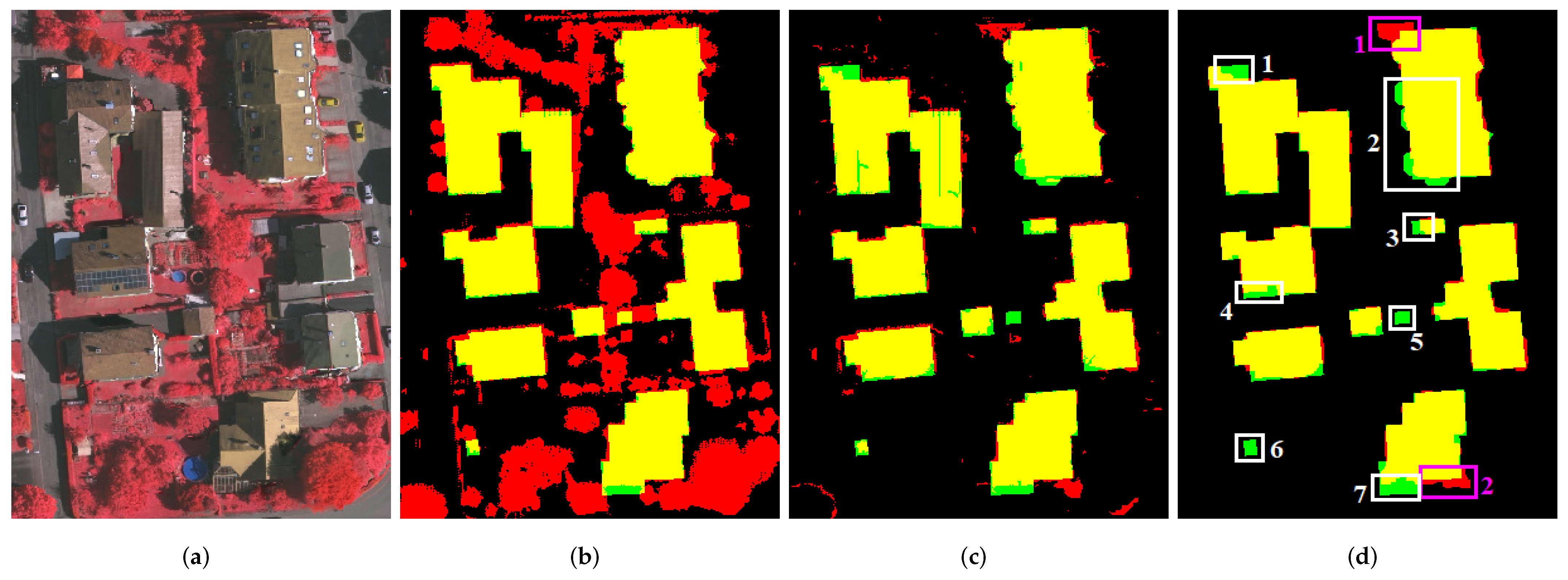
The initial building mask is generated by removing the vegetation detected by the eSH+eSH method or the iSH+eSH method from nDSM, as shown in Figure 1. Thus, we call our two initial building-mask-generation methods the beSH method and the biSH method (“b” denotes building).

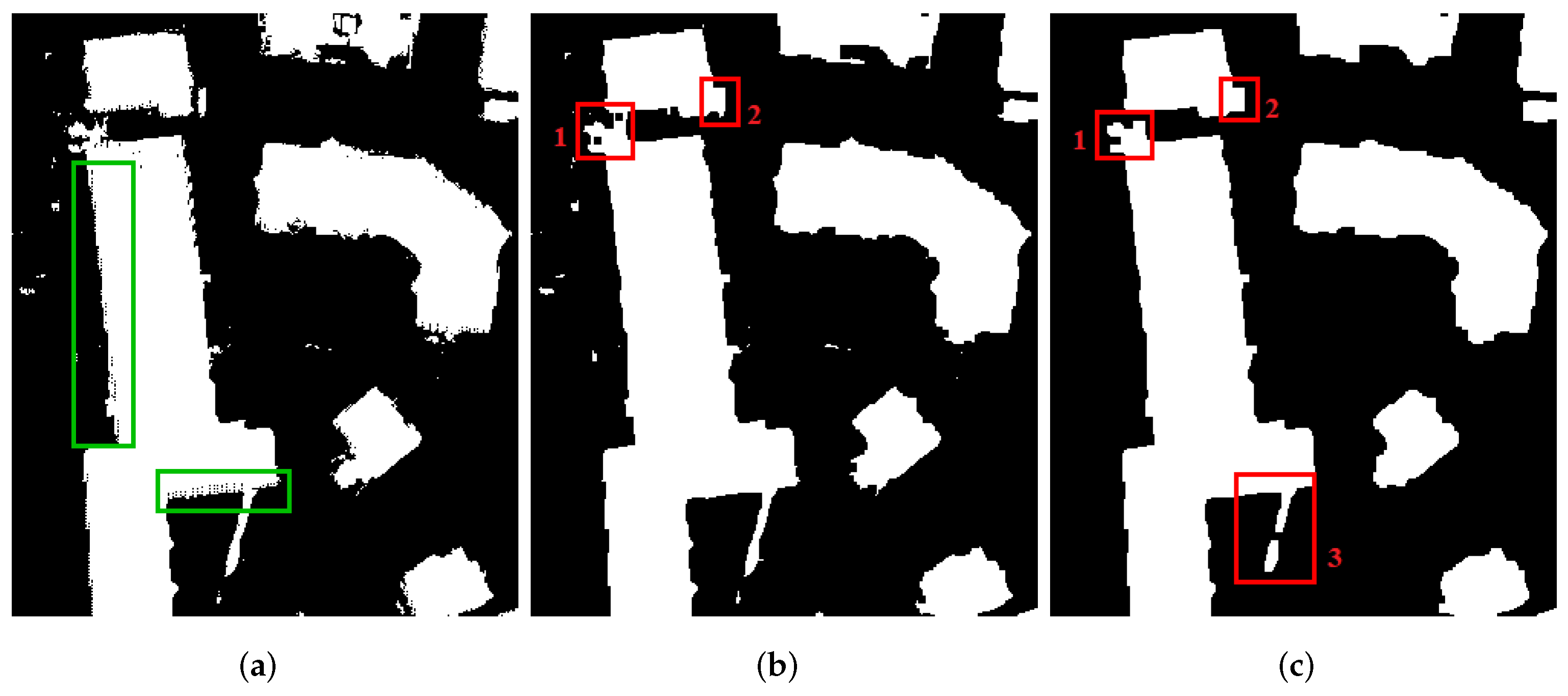
Because the improved vegetation detection methods have high accuracies, the initial building mask is already highly accurate. If we use the iSH+eSH method for vegetation detection (the results when using the eSH+eSH method are very similar), as shown in Figure 1d, in the initial building mask, most non-building points have been removed, and most building points have been retained; that is, the initial building mask correctly covers the main bodies of real buildings. However, the initial building mask has limitations, the main two of which are as follows:

(a). Parts of the building boundaries are determined by the nDSM generated from the LiDAR data, whereas parts are determined by the remote sensing image (because the vegetation information is extracted from the images). However, most boundaries determined by nDSM are not accurate because the density of LiDAR point clouds is generally not sufficiently large.

(b). Although the adopted vegetation detection methods are highly accurate, they are not perfect: a few vegetated areas may have not been detected, and a few building points may be misclassified as vegetation. Thus, there may still be some vegetation (in Figure 1d, some examples are marked by red rectangles) in the initial building mask, and some building points may have been incorrectly removed (in Figure 1d, some examples are marked by green rectangles).

After removing vegetation from the nDSM, most non-building points generally become disconnected and fragmentary, which may be easily resolved by morphological operations and region-size filtering. However, some of the remaining vegetated regions are large in size and may be connected to real buildings (see the regions marked by red rectangles in Figure 1d); thus, they are difficult to overcome using simple morphological operations and region-size filtering. In addition, morphological operations cannot remove the remaining vegetation points and simultaneously recover the missing building points, because removing the remaining vegetation points requires the morphological opening (or similar) operation, but recovering the missing building points requires the morphological closing (or similar) operation, which are two contradictory operations. Therefore, refining the initial building mask is not a trivial task.

2.2. Building Mask Refinement Based on Image Feature Consistency Constraints

Although building-mask refinement methods have been developed, they have limitations. Some methods adopt the features of LiDAR point clouds when refining building masks [30,35]. Thus, they inevitably incorporate inaccurate boundaries derived from the LiDAR data. Some methods attempt to project the initial building boundaries generated from LiDAR data onto the corresponding images and then use the boundaries or segments extracted from images to replace the initial coarse building boundaries [3,62,69]. This idea works theoretically but is difficult in practice. This idea requires precise matching between boundaries or between segments, but the correspondence between the boundaries of the initial building mask and the boundaries extracted from the images may not be good, making matching difficult. In addition, existing unsupervised boundary detection and segment detection methods are not sufficiently mature to obtain optimal results automatically, which leads to a dilemma: if strict parameters are used for the boundary detection or segment detection algorithm, the necessary boundaries or segments may not be retained; if loose parameters are used, too many boundaries or segments may be detected, which will increase the difficulty of matching boundaries or segments.

We also adopt the strategy of using image-derived boundaries to replace LiDAR-derived boundaries, but through region matching instead of boundary matching. Region matching is much less difficult than boundary matching and hence much more stable; thus, accurate results may be obtained automatically. Furthermore, it is easy to combine multiple matching results to further improve the refinement result if the strategy of region matching is adopted.

Specifically, the fundamental underpinning our method can be described as follows: the image features (including the spectral features and the texture features) of one building or one building part should be internally consistent, and through image segmentation we can obtain these regions with consistent image features. Because these segmentation regions have high overlap (matching degree) with the initial building regions, by computing the union of these segmentation regions with high matching degrees, we can replace the LiDAR-derived boundaries with the image-derived boundaries; that is, obtain the building mask with accurate boundaries. If the threshold for the matching degree is not very high, our method can also recover incorrectly removed building points. Because the adopted vegetation detection methods are highly accurate, each of the connected vegetated regions remaining in the initial building mask is only a small portion of the real connected vegetation region; thus, our method can also remove the remaining vegetation regions with large size, regardless of whether they are close to the real buildings.

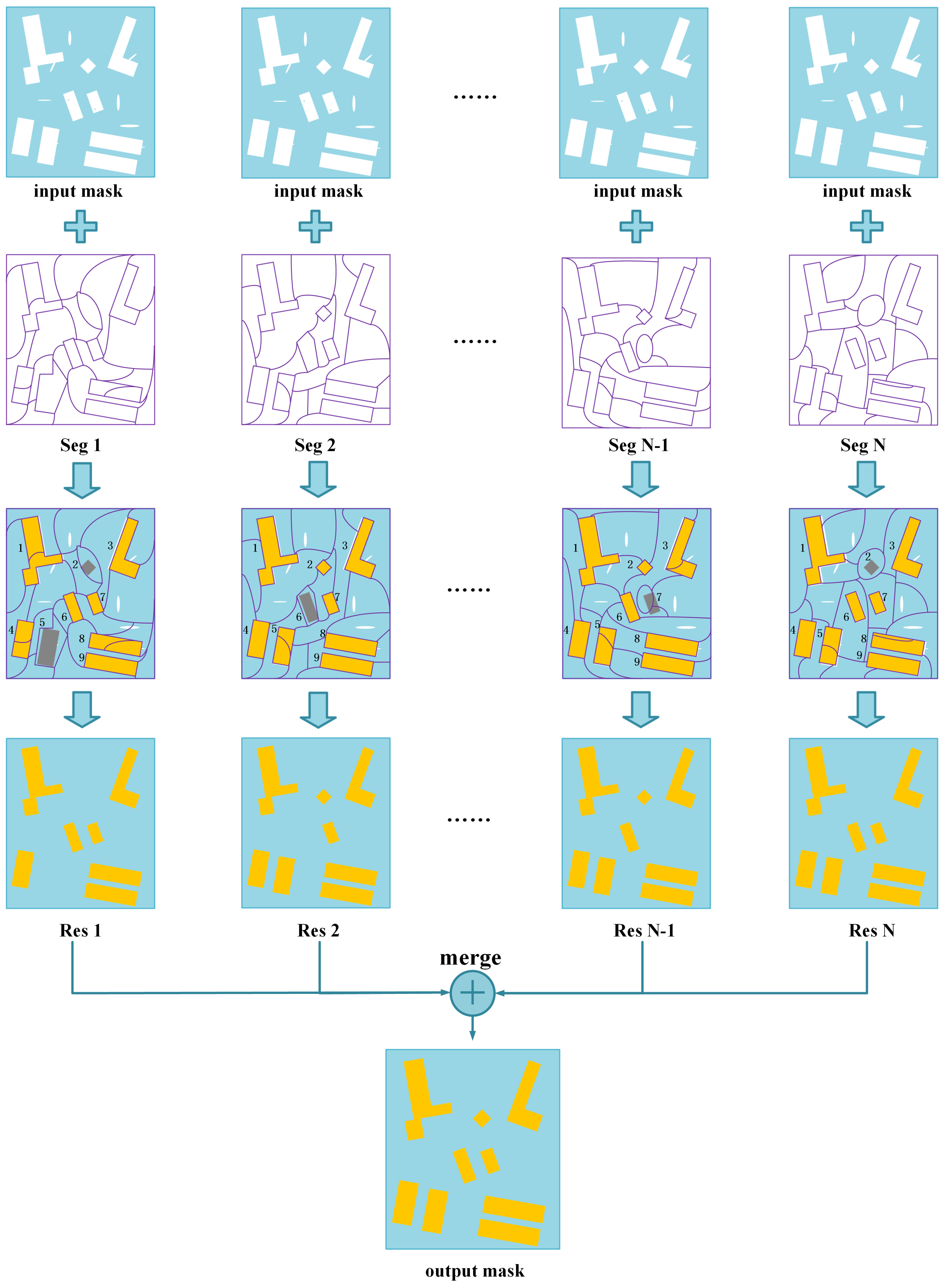
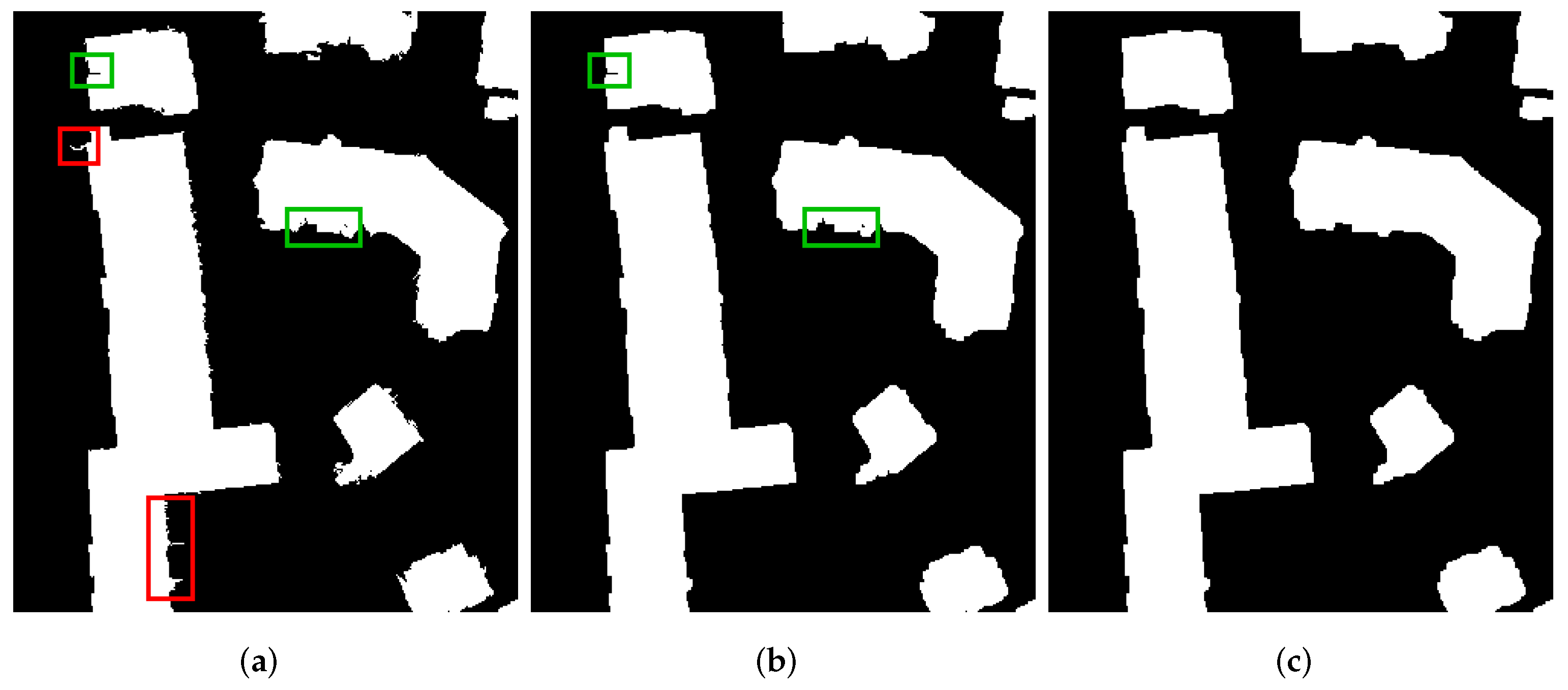
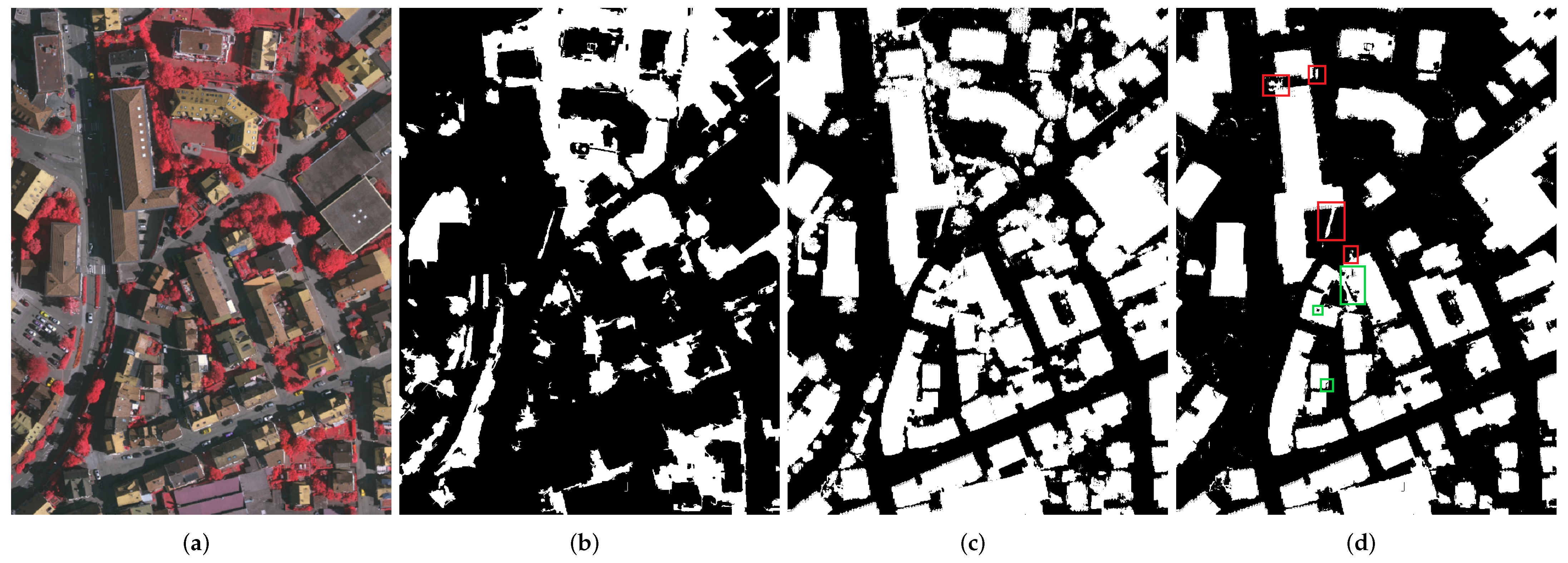
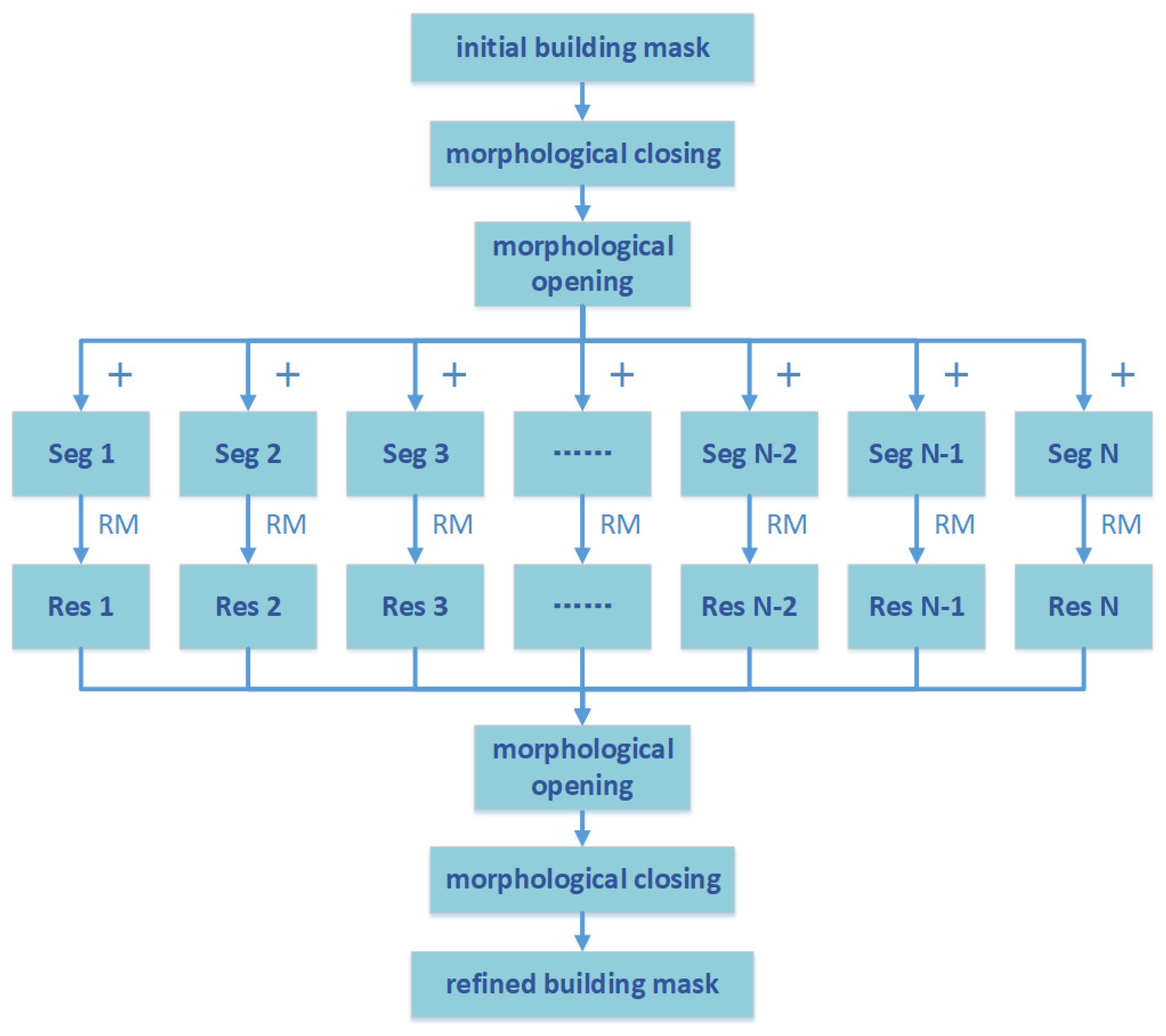
The workflow of our building-mask refinement method is shown in Figure 2. To better recover the missing building points (in Figure 3a, some examples are marked by green rectangles), before region matching, the morphological closing operation is performed on the initial building mask. However, this operation may also recover some non-building points (mostly vegetation points; in Figure 3b, some examples are marked by red rectangles). To counteract this side effect, the morphological opening operation is also performed, which can also remove the small-area non-building regions remaining in the initial building mask (Figure 3c is much clearer than Figure 3a,b). The first-closing-then-opening operation can mainly recover the missing building points as expected, as shown in Figure 3. However, the above preprocessing steps may introduce some unwanted points (see the region marked by the second red rectangle in Figure 3b,c), and some large non-building regions are still not removed (see the regions marked by the first and third red rectangles in Figure 3c).

Next, for region matching, three superpixel segmentation methods are adopted: the graph-based image segmentation (GS) algorithm [80], the simple linear iterative clustering (SLIC) algorithm [81], and the entropy rate superpixel segmentation (ERS) algorithm [82]. The GS algorithm [80] is an adaptive graph-based region growing method, which can lower the threshold for merging pixels in low-contrast regions and raise it in high-contrast regions. The SLIC algorithm [81] is essentially a K-means method that searches for pixels belonging to a cluster in a local space to reduce the computational cost. The ERS algorithm [82] is also a graph-based method, trying to maximise an objective function composed of two parts: the entropy rate of a random walk that encourages the superpixels to have compact shapes, and a balancing term that encourages the superpixels to have equal size. The input to the three segmentation algorithms is only the remote sensing image. All three segmentation algorithms have certain parameters to be set. However, we only need over-segmentations of the image, not the optimal segmentations. Therefore, the parameters are easy to set, and we can consider the three segmentation algorithms to be automatic methods. Notably, the SLIC and ERS algorithms both have the parameter of the number of superpixels, which may vary greatly for images with different resolutions or sizes. To make these two algorithms work automatically, we set this parameter to the superpixel number of the GS algorithm.

It should be pointed out that there are two segmentation types in this paper: semantic segmentation and non-semantic segmentation. Semantic segmentation methods assign a semantic label to each pixel/point in the image/LiDAR data. The building extraction, vegetation detection, shadow detection, and DEM extraction involved in this paper can all be regarded as semantic segmentation tasks. However, the GS, SLIC and ERS algorithms used for region matching are non-semantic segmentation methods. They are used to generate disjointed homogeneous regions (superpixels), each corresponding to an object or a part of it, but we do not know the semantic label of each superpixel. Generally, the non-semantic segmentation methods do not need to be trained, i.e., they are unsupervised methods. In contrast, most state-of-the-art semantic segmentation methods are supervised deep learning methods.

The thresholds of the matching degrees for the GS and ERS algorithms are both set to 0.85; thus, a segmentation region (superpixel) is considered a building or building part only when the portion of initial building pixels in it exceeds 85%. The threshold of the matching degrees for the SLIC algorithm is set to 0.90, because the maximum colour distance in the SLIC algorithm may vary significantly from image to image, but the authors of SLIC simply fixed it to a constant value; we conceive that such a setting will make the SLIC algorithm unable to adhere well to the boundaries for some images and that raising the region-matching threshold can help prevent the less accurate segmentation regions generated by the SLIC algorithm from appearing in the final building mask.

The workflow of the region-matching part of our method is presented in Figure 4 to explain the fundamental clearly. In the input building mask (see the first row of Figure 4), the buildings are marked by the colour white, while the background is marked by a light blue colour. N non-semantic segmentation algorithms are used for the region matching, where the boundaries of the segmentation regions are marked by a purple colour (see the second row of Figure 4) and each four-connected region enclosed by purple boundaries is a segmentation region. Then, each of the non-semantic segmentation results is superimposed on the input building mask, respectively, to compute the matching degrees (see the third row of Figure 4). Segmentation regions with high matching degrees are marked by a yellow color, while segmentation regions with not-high matching degrees are still marked by the original light blue colour. For example, for the first non-semantic segmentation algorithm (see the third row and the first column of Figure 4), the segmentation regions corresponding to the first, third, fourth, and sixth to ninth buildings have high matching degrees and are marked with a yellow colour, while the segmentation regions corresponding to the the second and the fifth buildings have low matching degrees and are marked by a light blue colour. Segmentation regions with high matching degrees are regarded as buildings (see the fourth row of Figure 4). However, none of the existing non-semantic segmentation algorithms are perfect and some of the segmentation regions will not match the corresponding buildings in the input building mask well (see the segmentation regions corresponding to the grey buildings in the third row of Figure 4). Therefore, each single region-matching result will probably miss some buildings or building parts (see the fourth row of Figure 4). So, we compute the union of the all the region matching results to get a complete building mask (see the last row of Figure 4).

To retain the real buildings, the segmentation regions corresponding to them should be optimally segmented or oversegmented. For example, in the third row and the first column of Figure 4, segmentation regions corresponding to the third, sixth, seventh, and ninth buildings are optimally segmented, with each segmentation region matching a real building well; while the segmentation regions corresponding to the first, fourth, and eighth buildings are oversegmented, with each segmentation region matching only a building part. In both cases, the real buildings can be retained. However, if one segmentation region is undersegmented, i.e., it corresponds to a building (or a building part) plus many other object pixels (see the segmentation regions corresponding to the grey buildings in the third row of Figure 4), the corresponding building will be missing in the region-matching result. In fact, optimal segmentation result is very challenging to generate automatically, but oversegmentation results are very easy to obtain and their generation can be regarded as an automatic process. Therefore, to obtain a satisfactory region matching result, we use oversegmentation instead of the optimal segmentation. Note that we use segmentation regions instead of superpixels when depicting the workflow of the region matching because, generally, superpixels mean oversegmented regions [83], but we are not assuming regions are oversegmented before we reach the above conclusion.

The number N in Figure 2 and Figure 4 does not have to be set to three, which means that we do not have to use three non-semantic segmentation algorithms. More segmentation algorithms can be used to obtain better refinement results, which, however, means a higher computational cost is required. We utilise only three segmentation algorithms to guarantee the accuracy of the refinement and simultaneously guarantee the processing efficiency. The segmentation algorithms also do not have to be the three algorithms that we adopt. However, we should note that the segmentation results can influence the refinement accuracy. The segmentation algorithms used should be sensitive to the details in the images to differentiate the building parts and non-building parts in shadowed areas or other areas with low contrast. Both the GS and ERS algorithms fulfil the requirement. The SLIC algorithm may fail in some cases, and we use a higher matching threshold to address these adverse situations.

If a segmentation algorithm can generate the optimal segmentation result, then we can use only this algorithm instead of three or more algorithms to perform region matching, and the refinement method becomes the popular object-based method [84,85]. However, none of the existing non-semantic segmentation algorithms are perfect so far. Hence, the segmentation regions of one algorithm cannot correspond to all the real building regions well. Thus, the region-matching result will miss some building parts when the threshold for the matching degree is high. Lowering the threshold can overcome the problem of missing detection (underdetection), but this will probably introduce some unrelated points to the building mask and thus cannot realise the goal of refinement. The thresholds for the matching degree of our method are high, and thus it can effectively avoid incorporating unrelated points, and computing the union of the matching results of multiple segmentation algorithms can also overcome the problem of missing detection.

Notably, although we only need each non-semantic segmentation of the remote sensing image to be an oversegmentation, the segmentation regions of this oversegmentation cannot be too small, otherwise the refinement functionality of the region matching would be weakened. In extreme cases, assuming that each segmentation region contains only one pixel, the refined mask will be just the initial building mask regardless of the tuning of the threshold for the region matching (still in the range of (0, 1]).

The morphological closing operation performed before the region matching may have caused the final building mask to incorporate some unrelated points near the boundaries. The imperfect non-semantic segmentation algorithm we used may also lead to some small-area elongated false building regions (some examples are marked by the red rectangles in Figure 5a), and some underdetection (some examples are marked by the green rectangles in Figure 5a). To eliminate these non-building points, morphological opening operation is performed after the region matching. However, this opening operation may worsen the underdetection problem (some examples are marked by the green rectangles in Figure 5b). To counteract this side effect, a morphological closing operation is performed after it. After this first-opening-then-closing postprocessing, the building mask looks much better.

After all the aforementioned steps, the remaining non-building points become disconnected and fragmentary, which can be easily removed through region size filtering. In this study, connected regions smaller than 2.5 ${\mathrm{m}}^2$ are regarded as non-building points and thus removed.

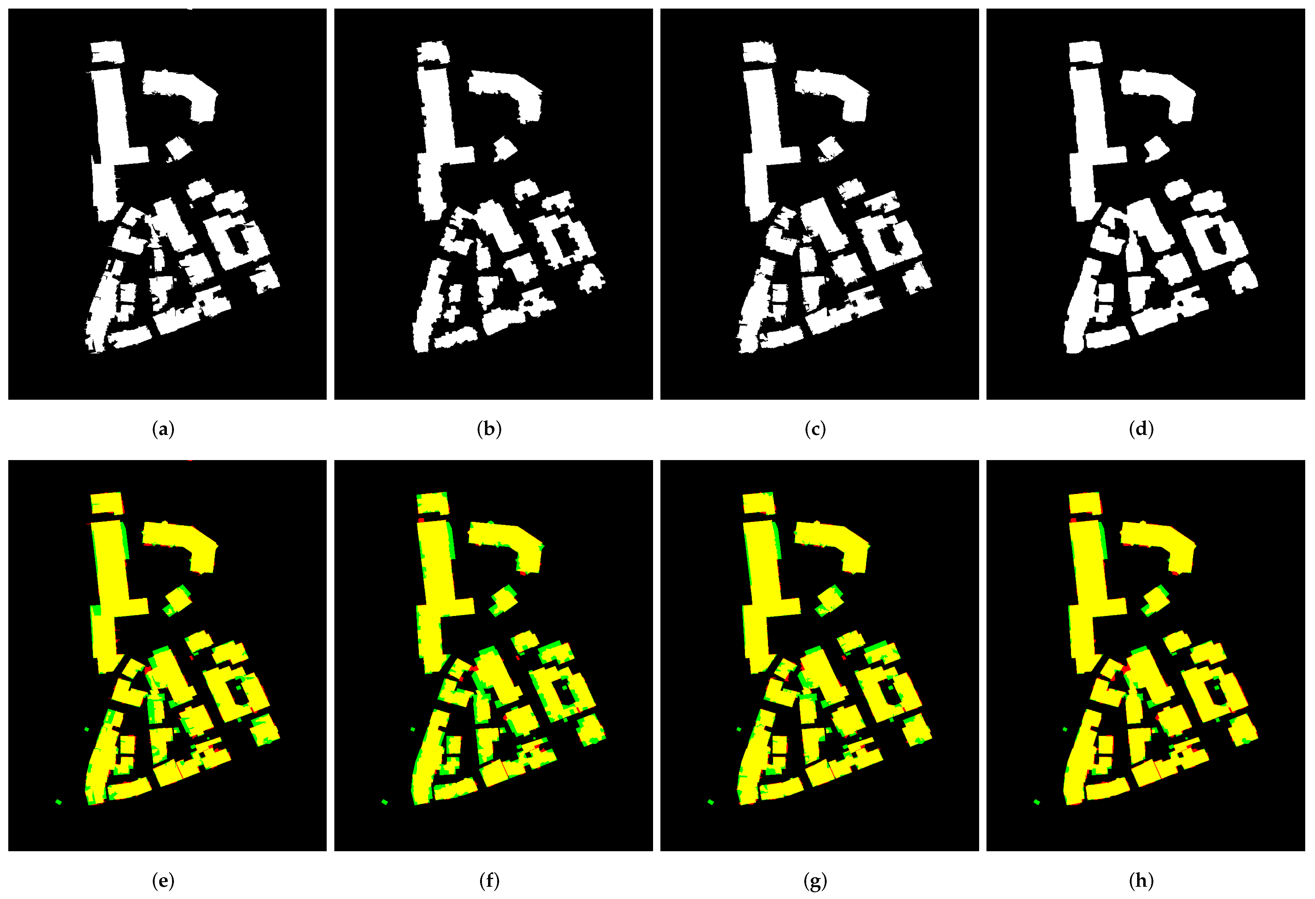
Figure 6 presents an illustration of our building-mask refinement method on the first test area of the Vaihingen dataset, for which the initial building mask is generated using our biSH method (see Figure 1d). We can see that the matching result of each non-semantic segmentation algorithm has accurate boundaries, and most of the remaining vegetated regions have been successfully removed, but each single matching result misses some real building parts. However, the union of the three matching results has relatively complete building regions and accurate boundaries, and most of the vegetated regions remaining in the initial building mask have also successfully been removed.

We call our building-mask refinement method the IFCC method, in which IFCC denotes the image feature consistency constraint, and we call our building extraction methods (including the initial building mask generation stage and the building-mask refinement stage) the beSH+IFCC method and the biSH+IFCC method. The premise of our IFCC method is that the initial building mask has high accuracy. Therefore, in addition to the proposed beSH and biSH methods, it can be combined with other accurate building extraction methods.

3. Experimental Results and Discussion

To validate the effectiveness of the proposed building extraction methods, we compared them with 29 methods in this section. The comparison has two parts: (1) a qualitative and quantitative comparison with three state-of-the-art methods (Section 3.3) and (2) a quantitative comparison with publicly available evaluation results (Section 3.4). The test data and evaluation metrics are introduced in Section 3.1, the experimental setup is detailed in Section 3.2, and the related discussions are presented in Section 3.5.

For the first comparison, our methods were compared with three state-of-the-art methods both qualitatively and quantitatively: DeepLabv3+ [86], U-Net [87] and the hierarchical overlay analysis (HOA) method [30]. We chose DeepLabv3+ and U-Net because they are two of the most popular state-of-the-art deep-learning architectures for semantic segmentation. The HOA method was chosen because it is a recently developed unsupervised method that also attempts to generate initial building masks by removing vegetation points from nDSM and then refine the initial building masks.

For the second comparison, our methods were qualitatively compared with 26 existing methods: 10 of them are the top-10 methods in area quality that have evaluation results for all three test areas of the Vaihingen dataset on the official website of the ISPRS Test Project on Urban Classification and 3D Building Reconstruction (website link: https://www2.isprs.org/commissions/comm2/wg4/results, accessed on 28 February 2022), and the other 16 of them are state-of-the-art methods published in the last five years (2017–2021). Notably, there are another six deep-learning methods among the 16 state-of-the-art methods; thus, there are eight deep-learning methods compared with our methods in this paper.

3.1. Test Data and Evaluation Metrics

We adopted the Vaihingen dataset of the ISPRS [72] to evaluate all the compared methods, which comprises 33 orthorectified remote sensing images and the corresponding LiDAR point clouds. The images have three bands: the green, red, and near-infrared bands, from which we can compute the NDVI and NDGI. The ISPRS has offered groundtruth for the vegetation and the buildings, and has designated three test areas from the 33 images: the first test area (Figure 7a) mainly contains historic buildings with complex shapes, the second test area (Figure 8a) mainly contains high-rise residential buildings surrounded by trees, and the third test area (Figure 9a) mainly contains small detached buildings. Except that all test areas contain some vegetation (the vegetation all appears red in a false colour format), the buildings in the three test areas differ significantly in their shapes, colours, sizes, and backgrounds. Even for vegetation, which is part of the background, the three test areas also show different characteristics: the first test area has relatively less vegetation compared to the other two test areas, the second test area has many trees, and the third has many bushes and lawns. Thus, the three test areas are challenging for unsupervised building extraction methods if a high accuracy is required.

To evaluate the building extraction results quantitatively, we adopted the evaluation metrics suggested by the ISPRS [88]. Therefore, we adopted 12 metrics for building extraction: the area completeness, area correctness, and area quality (abbreviated as ${\mathrm{Com}}_{\mathrm{ar}}$, ${\mathrm{Cor}}_{\mathrm{ar}}$ and ${\mathrm{Q}}_{\mathrm{ar}}$, respectively); the object completeness, object correctness, and object quality when only considering buildings larger than 10 ${\mathrm{m}}^2$ (abbreviated as ${\mathrm{Com}}_{10}$, ${\mathrm{Cor}}_{10}$ and ${\mathrm{Q}}_{10}$, respectively); the object completeness, object correctness, and object quality when only considering buildings larger than 50 ${\mathrm{m}}^2$ (abbreviated as ${\mathrm{Com}}_{50}$, ${\mathrm{Cor}}_{50}$ and ${\mathrm{Q}}_{50}$, respectively); and the object completeness, object correctness, and object quality when considering buildings of larger than 2.5 ${\mathrm{m}}^2$ (abbreviated as ${\mathrm{Com}}_{\mathrm{obj}}$, ${\mathrm{Cor}}_{\mathrm{obj}}$ and ${\mathrm{Q}}_{\mathrm{obj}}$, respectively). According to the convention [30,89], we ranked all the compared methods by their area quality ${\mathrm{Q}}_{\mathrm{ar}}$.

Completeness measures the proportion of correctly extracted buildings over real buildings, which is also called recall [71,90], and is defined as Formula (7). Correctness measures the proportion of the correctly extracted buildings over the extracted buildings, also called precision [71,90], and is defined as Formula (8). Quality is the overall evaluation metric, also called intersection over union (IoU) [34], and is defined as Formula (9).

$$\mathrm{Completeness}=\frac{\mathrm{TP}}{\mathrm{TP}+\mathrm{FN}},$$

(7)

$$\mathrm{Correctness}=\frac{\mathrm{TP}}{\mathrm{TP}+\mathrm{FP}},$$

(8)

$$\mathrm{Quality}=\frac{\mathrm{TP}}{\mathrm{TP}+\mathrm{FP}+\mathrm{FN}},$$

(9)

where TP (true positive) denotes the correctly extracted building pixels or building objects (for the object-level evaluation); FN (false negative) denotes the missing building pixels or building objects, that is, building pixels or building objects that are buildings but not extracted; and FP (false positive) denotes the incorrectly extracted building pixels or building objects, that is, the pixels or objects that are not buildings but extracted as buildings.

To compare the vegetation detection methods, we also used the overall accuracy (OA, defined as Formula (10)) and ${\mathrm{F}}_1$ score (defined as Formula (11)). Of course, we can also use quality to assess the vegetation detection results. In this study, we used different metrics for the two tasks to maintain accordance with the literature on the two tasks.

$$\mathrm{OA}=\frac{\mathrm{TP}+\mathrm{TN}}{\mathrm{TP}+\mathrm{TN}+\mathrm{FP}+\mathrm{FN}}.$$

(10)

$${\mathrm{F}}_1=\frac{\mathrm{Completeness}\times \mathrm{Correctness}}{\mathrm{Completeness}+\mathrm{Correctness}}.$$

(11)

3.2. Experimental Setup

This section presents the experimental setup details in this paper. For our methods and the HOA method, the DEM is extracted using the lasground module of the publically available LAStools software. The other functions of the HOA method are deployed by using its Matlab source code used in the reference of [30], and the parameters are set to the default values as suggested by its authors. The vegetation detection in our methods is implemented by modifying the Matlab source code used in the reference of [71]. The GS, SLIC, and ERS segmentation algorithms used in our methods were deployed by using the source code released by their authors, and the download links are as follows: http://cs.brown.edu/people/pfelzens/segment/ (accessed on 28 February 2022) for the GS algorithm; https://www.epfl.ch/labs/ivrl/research/slic-superpixels/ (accessed on 28 February 2022) for the SLIC algorithm; and https://github.com/mingyuliutw/EntropyRateSuperpixel (accessed on 28 February 2022) for the ERS algorithm.

As for the two compared deep-learning methods, we split the whole Vaihingen dataset into tiles sized 512 × 512 pixels and manually selected the patches covering the three test areas of the Vaihingen dataset as the test data. Random rotation and random crop were applied to augment the training dataset. Finally, there were 2720 training tiles and 12 test tiles. We implemented DeepLabv3+ [86] and U-Net [87] based on the PyTorch library. Experiments were conducted on a desktop computer with a 24 GB NVIDIA GeForce RTX 3090 graphics card. The binary cross entropy loss function and the Adam optimiser were selected to optimise the two deep-learning models. The batch size of DeepLabv3+ is 16 and 8 for U-Net. We concatenated the high-resolution optical remote sensing image and the nDSM as model input and trained the two deep-learning models from scratch. DeepLabv3+ achieved the best performance after 14,450 iterations, while U-Net converged after 11,900 iterations.

3.3. Qualitative and Quantitative Comparison with the State-of-the-Art Methods

For the first comparison, all three test areas of the Vaihingen dataset were used as example images. When we compared our two methods with the HOA method, in addition to the three test areas, a large orthorectified image stitched by all 33 single images was used to maintain accordance with the work of [30], which we call the entire dataset. We used the area quality of the three methods on the entire dataset as the final evaluation criterion to rank them. Note that the entire dataset contains the test areas. Therefore, the comparison on the entire dataset is more reasonable and complete than that on just the three test areas. However, we used a large portion of the entire dataset to train DeepLabv3+ and U-Net; therefore, comparing them with our methods on the entire dataset is not fair and we only used the three test areas to compare with them.

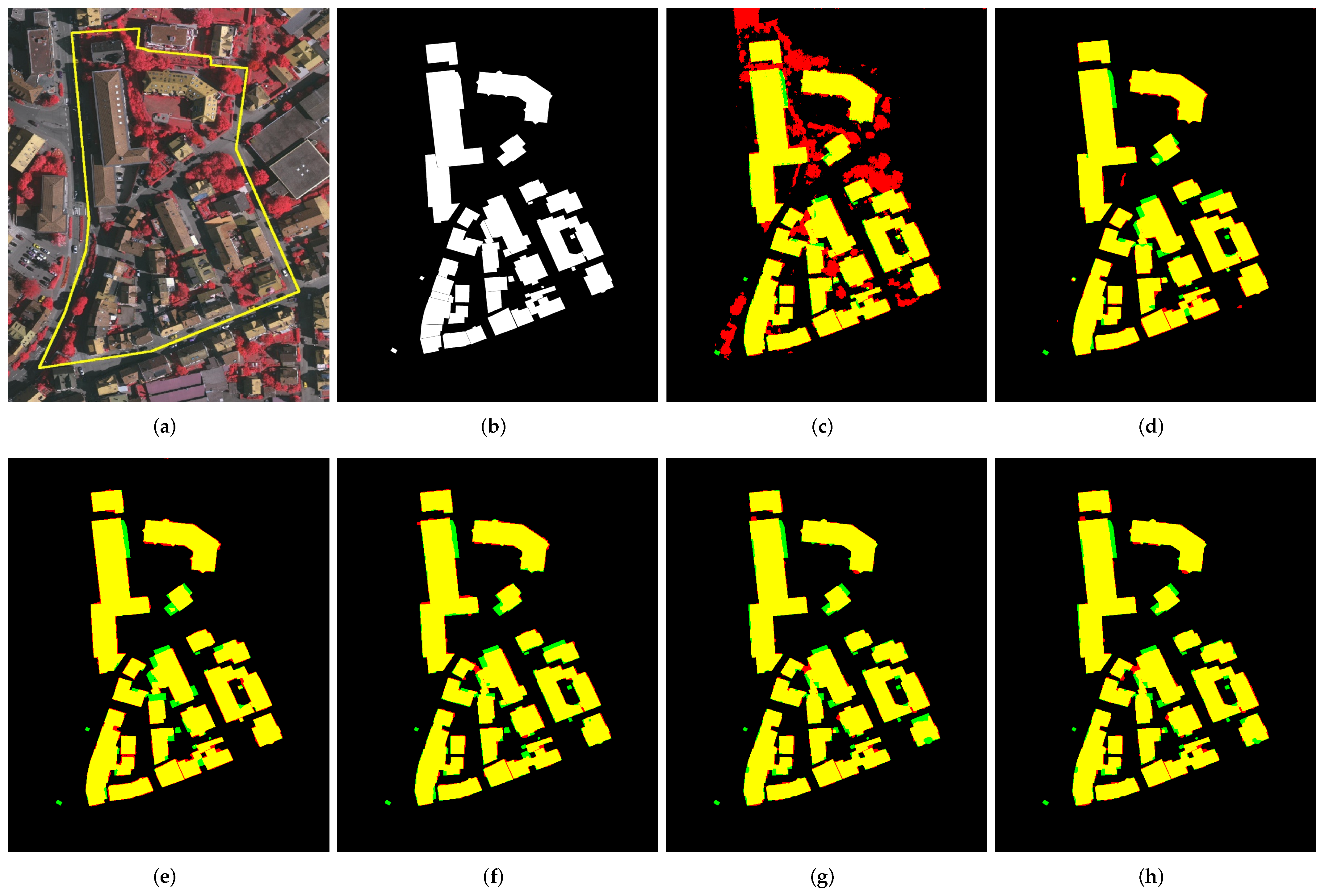
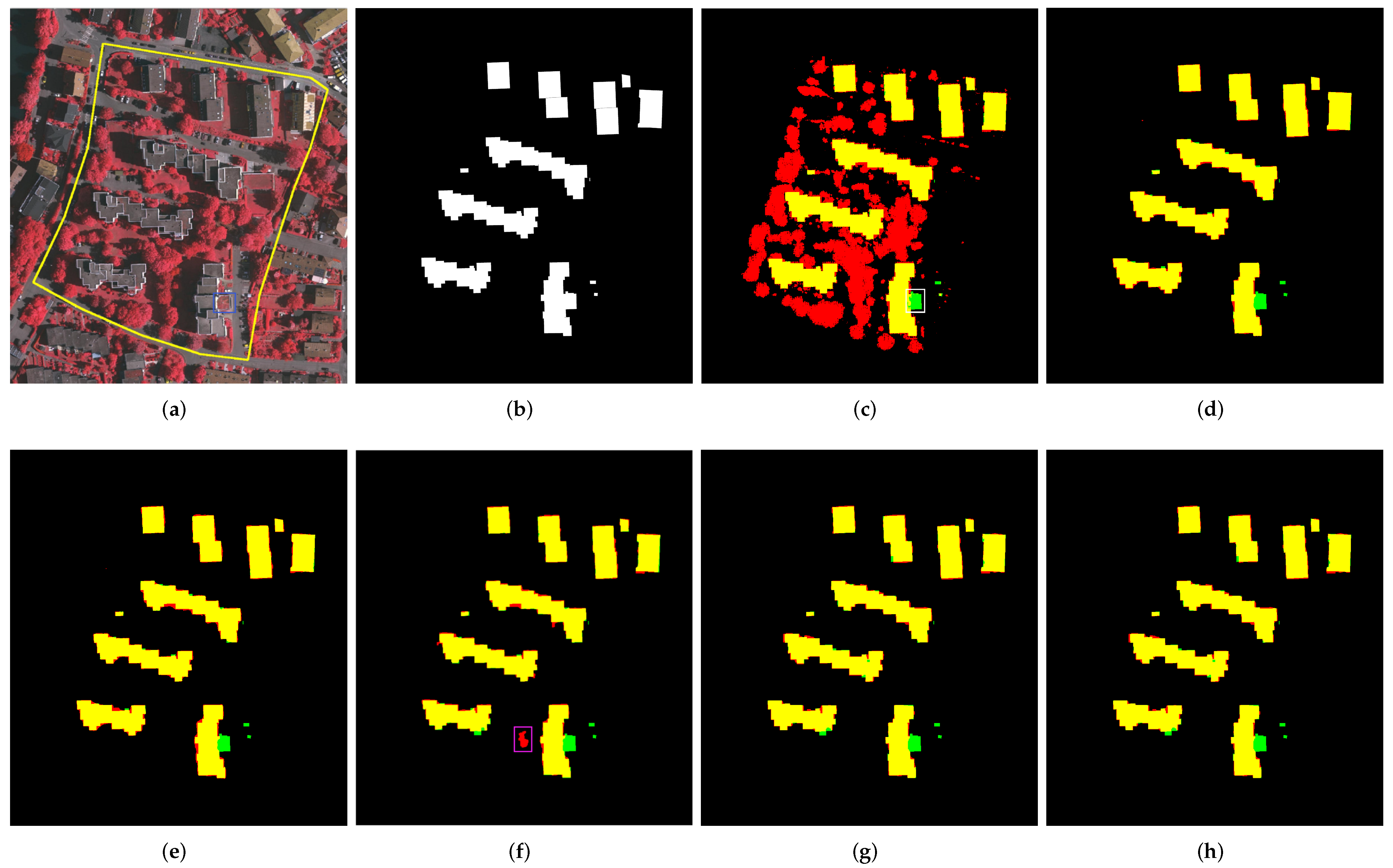
The comparison results on the first test area are presented in Figure 7, where the range of the test area is marked by the yellow polyline on the orthorectified image (Figure 7a). The nDSM that has been binarised by the moment-preserving method [73] is also presented to better analyse the comparison, temporarily supposing it is a building extraction result. For the results of all methods, correct detection, false detection (over-detection), and missing detection (under-detection) are marked by yellow, red and green colours, respectively. The above operations also suit the comparison on the other two test areas (Figure 8 and Figure 9).

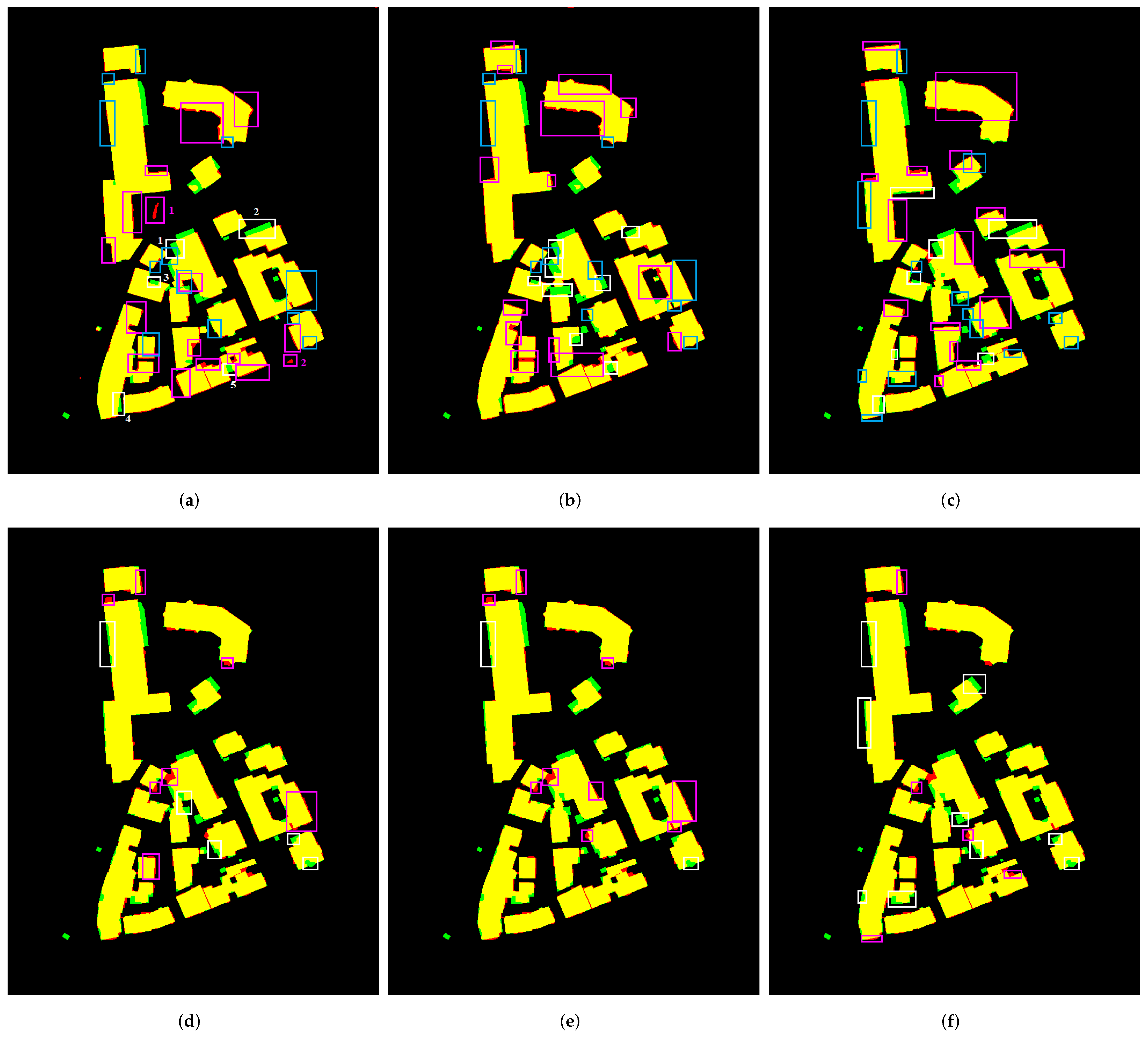
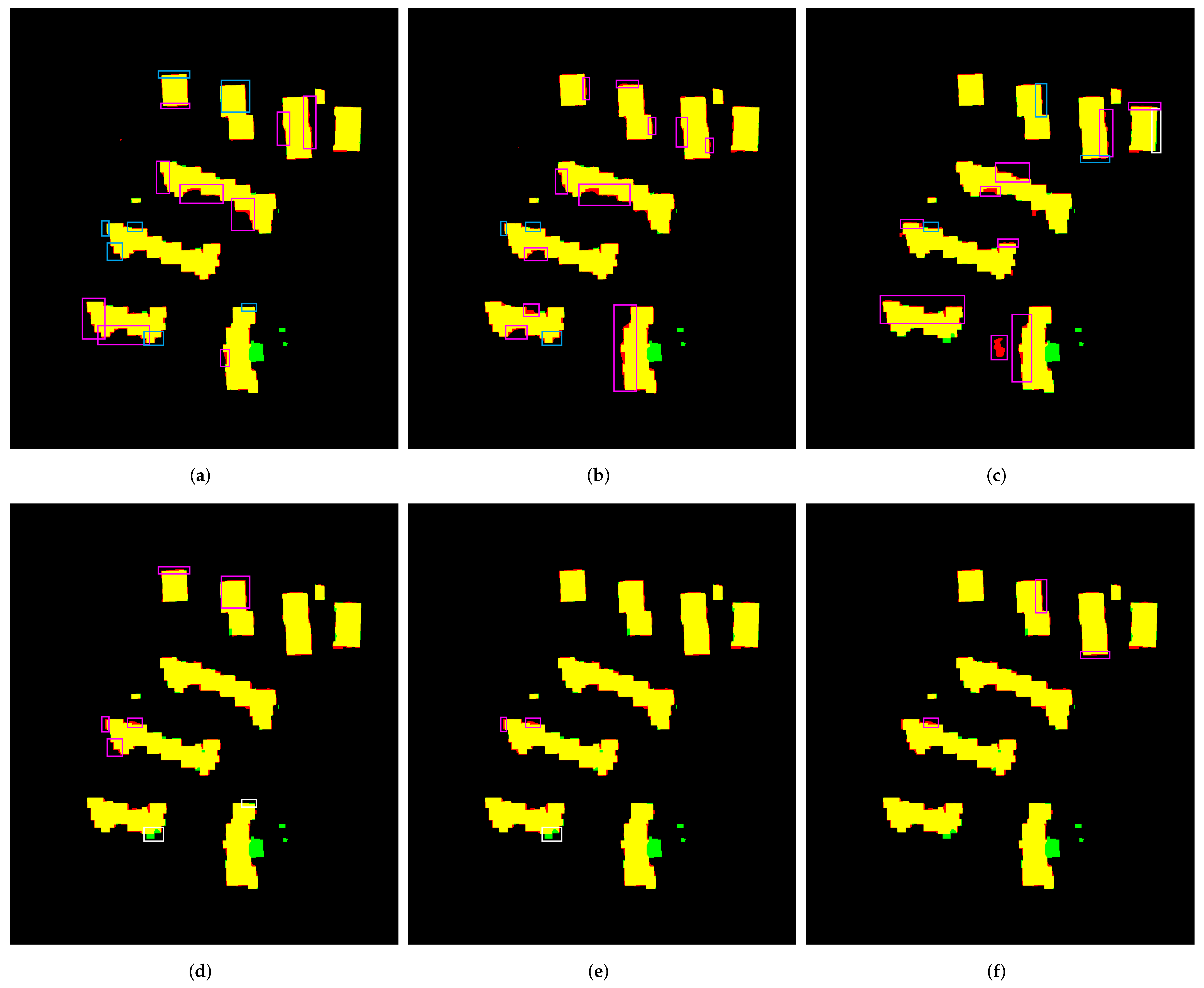
As shown in Figure 7, all the compared methods (except the nDSM) obtained good results but had some overdetected regions and missing regions. Deciding which result is better is difficult if we only compare them roughly, because they all obtain better results in some regions but perform worse in other regions. So in Figure 10a–c, for the results of DeepLabv3+, U-Net, and the HOA method, we marked the ultra overdetected regions with magenta rectangles compared with the proposed biSH+IFCC method, the ultra missing regions with white rectangles compared with the proposed biSH+IFCC method, and the regions where they performed better than the proposed biSH+IFCC method with blue rectangles. In Figure 10d–f, for the result of our biSH+IFCC method, we marked the ultra overdetected regions with magenta rectangles, the ultra missing regions with white rectangles compared with DeepLabv3+ (in Figure 10d), U-Net (in Figure 10e), and the HOA method (in Figure 10f), respectively. The rectangles in Figure 10d (or Figure 10e or Figure 10f) correspond to the blue rectangles in Figure 10a (or Figure 10b or Figure 10c). To clarify the comparison, we marked only the main differences. The same operations were applied to the other two test areas (Figure 11 and Figure 12).

As shown in Figure 10a, for the overdetection problem, compared with the biSH+IFCC method, DeepLabv3+ extra misclassifies a large vegetated region (see the red region marked by the first magenta rectangle) and a car (see the red region marked by the second magenta rectangle) as buildings, and the other ultra overdetection mainly occurs at the building boundaries. For the underdetection problem, compared with the biSH+IFCC method, it mainly misses another two large building parts (see the green regions marked by the first two white rectangles) and another three relatively small building parts (see the green regions marked by the third, fourth, and fifth white rectangles). It also performs better than the biSH+IFCC method in some regions, the main part of which is marked by the blue rectangle in Figure 10a. The comparison of U-Net and the HOA method with our biSH+IFCC method is similar to that of the DeepLabv3+, except that the ultra overdetection of U-Net and the HOA method mainly occurs at the building boundaries, which, however, is much worse than that of DeepLabv3+. Because the areas where the two deep learning methods and the HOA method make errors are larger than our methods, we consider that our methods perform a little better. As for the comparison of the proposed beSH+IFCC and biSH+IFCC methods, we consider that their results are very similar. Therefore, the comparison of DeepLabv3+, U-Net and the HOA method with the beSH+IFCC method should be very similar to that with the biSH+IFCC method. For this reason, we only presented the rectangle-marked comparison results with the biSH+IFCC method, which also suits the comparison on the other two test areas.

The quantitative evaluation results in

Table 1. Quantitative evaluation results of different methods on the first test area.

Method	${\mathbf{Com}}_{\mathbf{ar}}$	${\mathbf{Cor}}_{\mathbf{ar}}$	${\mathbf{Q}}_{\mathbf{ar}}$	${\mathbf{Com}}_{10}$	${\mathbf{Cor}}_{10}$	${\mathbf{Q}}_{10}$	${\mathbf{Com}}_{50}$	${\mathbf{Cor}}_{50}$	${\mathbf{Q}}_{50}$
DeepLabv3+	95.07%	94.23%	89.84%	100.00%	95.00%	95.00%	100.00%	100.00%	100.00%
U-Net	94.29%	93.65%	88.63%	96.88%	100.00%	96.88%	100.00%	100.00%	100.00%
HOA	93.08%	95.00%	88.73%	93.75%	100.00%	93.75%	100.00%	100.00%	100.00%
nDSM	96.03%	71.41%	69.36%	100.00%	46.67%	46.67%	100.00%	63.64%	63.64%
beSH+IFCC	93.34%	95.95%	89.81%	96.88%	100.00%	96.88%	100.00%	100.00%	100.00%
biSH+IFCC	93.90%	95.74%	90.13%	96.88%	100.00%	96.88%	100.00%	100.00%	100.00%

also validate our visual comparison, and the ranking of area quality is as follows: the proposed biSH+IFCC method, DeepLabv3+, the proposed beSH+IFCC method, the HOA method and U-Net. Notably, in Table 1, the best results were marked in boldface, and the second-best results were marked by underlining, which also applies to the following tables in this section.

A visual inspection of the corresponding nDSM demonstrates that some building parts were already missing in the nDSM generation stage, which is why the HOA method and our two methods also miss these building parts, because the first step for all of them is to obtain the nDSM using LAStools. However, the completeness of the nDSM reaches 96.03%; thus, the nDSM generated by LAStools is highly complete for the subsequent building extraction.

The comparison on the second test area is simpler than that on the first test area because there were fewer buildings. The comparison results are presented in Figure 8, from which we can see that all compared methods (nDSM not included) obtained satisfactory extraction of the main bodies of the buildings, except that they all missed a large building part (see the green regions in the bottom-right corner in Figure 8d–h). The three unsupervised methods failed on this building part because this part was already missing in the nDSM (see the green regions marked by the white rectangle in Figure 8c). This results from the following: this part is of low height, which makes its extraction from LiDAR data difficult. In addition, the roof of this building part is full of vegetation, which also makes its spectral feature abnormal from common buildings, which is why both the two compared deep-learning methods also fail on this building part. Besides, the HOA method incorrectly detects a shadowed vegetation region of large size as buildings (see the red regions marked by the magenta rectangle in Figure 8f) because its vegetation detection method cannot well recognise vegetation in shadows. Our methods can detect shadows and recognise vegetation in shadows, and thus are not limited by such problems in this test area.

As shown in Figure 11, in terms of the boundaries, the DeepLabv3+ method performs best among all three methods compared with ours, with fewer overdetected pixels and fewer missing pixels. However, U-Net and the HOA method have more overdetected pixels near the boundaries. The quantitative evaluation results in

Table 2. Quantitative evaluation results of different methods on the second test area.

Method	${\mathbf{Com}}_{\mathbf{ar}}$	${\mathbf{Cor}}_{\mathbf{ar}}$	${\mathbf{Q}}_{\mathbf{ar}}$	${\mathbf{Com}}_{10}$	${\mathbf{Cor}}_{10}$	${\mathbf{Q}}_{10}$	${\mathbf{Com}}_{50}$	${\mathbf{Cor}}_{50}$	${\mathbf{Q}}_{50}$
DeepLabv3+	97.20%	93.59%	91.13%	100.00%	100.00%	100.00%	100.00%	100.00%	100.00%
U-Net	97.43%	91.95%	89.77%	100.00%	100.00%	100.00%	100.00%	100.00%	100.00%
HOA	96.37%	92.91%	89.77%	91.67%	100.00%	91.67%	100.00%	100.00%	100.00%
nDSM	97.69%	44.06%	43.60%	100.00%	21.43%	21.43%	100.00%	29.41%	29.41%
beSH+IECC	96.47%	94.01%	90.89%	100.00%	100.00%	100.00%	100.00%	100.00%	100.00%
biSH+IFCC	96.46%	94.18%	91.03%	100.00%	100.00%	100.00%	100.00%	100.00%	100.00%

are in accordance with the aforementioned visual comparison, with the ranking by area quality as follows: DeepLabv3+, the biSH+IFCC method, the beSH+IFCC method, the HOA method (area quality corrected to four decimal places: 89.7726%), and U-Net (area quality corrected to four decimal places: 89.7678%). Notably, our method also obtains higher object quality values when only considering objects larger than 10 ${\mathrm{m}}^2$ than the HOA method because it incorrectly treats a vegetated region larger than 10 ${\mathrm{m}}^2$ as a building.

The comparison results on the third test area are presented in Figure 9, from which we can see that again, all the compared methods (nDSM not included) obtain acceptable detection results, and we cannot determine which one is better if we do not visually compare them carefully. As shown in Figure 9 and the rectangle-marked comparison in Figure 12, DeepLabv3+ obtains more better-performing areas (see the regions marked by blue rectangles in Figure 12a) than less effective areas (see the regions marked by white and magenta rectangles in Figure 12a); thus, it obtains better results than our methods. U-Net obtains an approximately equal amount of better-performing areas (see the regions marked by blue rectangles in Figure 12b) to the less effective areas (see the regions marked by the white and magenta rectangles in Figure 12b), which means it obtains comparable results to our methods. Compared with the biSH+IFCC method, except for missing another four big buildings or building parts (see the green regions marked by the first four white rectangles in Figure 12c) and misclassifying one large vegetation region as a building (see the red region marked by the first magenta rectangle in Figure 12c), the HOA method performs well on the main bodies of the buildings. However, it has too many coarse building boundaries, most of which are overdetection. The HOA method mainly shows advantages over our methods on the two buildings marked by the first four blue rectangles in Figure 12c, but our methods show obvious advantages over the HOA method on more buildings. Therefore, we conceive our methods outperform the HOA method on this test area.

The quantitative evaluation results in

Table 3. Quantitative evaluation results of different methods on the third test area.

Method	${\mathbf{Com}}_{\mathbf{ar}}$	${\mathbf{Cor}}_{\mathbf{ar}}$	${\mathbf{Q}}_{\mathbf{ar}}$	${\mathbf{Com}}_{10}$	${\mathbf{Cor}}_{10}$	${\mathbf{Q}}_{10}$	${\mathbf{Com}}_{50}$	${\mathbf{Cor}}_{50}$	${\mathbf{Q}}_{50}$
DeepLabv3+	95.06%	95.22%	90.72%	89.58%	100.00%	89.58%	100.00%	100.00%	100.00%
U-Net	95.53%	93.55%	89.63%	95.00%	100.00%	95.00%	100.00%	100.00%	100.00%
HOA	93.53%	93.61%	87.91%	83.33%	100.00%	83.33%	100.00%	100.00%	100.00%
nDSM	97.03%	64.73%	63.47%	95.83%	60.00%	58.47%	100.00%	80.00%	80.00%
beSH+IFCC	93.34%	95.94% 1	89.79%	91.67%	100.00%	91.67%	100.00%	100.00%	100.00%
biSH+IFCC	93.17%	95.94%	89.64%	91.67%	100.00%	91.67%	100.00%	100.00%	100.00%

¹ The Cor_ar values corrected to 3 decimal places for our beSH+IFCC and biSH+IFCC methods are 95.937% and 95.942%, respectively.

are in accordance with the aforementioned visual comparison, with the ranking of area quality as follows: DeepLabv3+, the beSH+IFCC method, the biSH+IFCC method, U-Net and the HOA method. Notably, our methods also obtain higher object quality when only considering objects larger than 10 ${\mathrm{m}}^2$ than the HOA method because it misses more buildings larger than 10 ${\mathrm{m}}^2$.

The average quantitative evaluation results on all three test areas are presented in

Table 4. Average quantitative evaluation results of different methods on the three test areas.

Method	${\mathbf{Com}}_{\mathbf{ar}}$	${\mathbf{Cor}}_{\mathbf{ar}}$	${\mathbf{Q}}_{\mathbf{ar}}$	${\mathbf{Com}}_{10}$	${\mathbf{Cor}}_{10}$	${\mathbf{Q}}_{10}$	${\mathbf{Com}}_{50}$	${\mathbf{Cor}}_{50}$	${\mathbf{Q}}_{50}$
DeepLabv3+	95.77%	94.35%	90.57%	97.22%	98.33%	95.56%	100.00%	100.00%	100.00%
U-Net	95.75%	93.05%	89.34%	95.49%	100.00%	95.49%	100.00%	100.00%	100.00%
HOA	94.33%	93.84%	88.80%	89.58%	100.00%	89.58%	100.00%	100.00%	100.00%
nDSM	96.92%	60.06%	58.81%	98.61%	42.70%	42.19%	100.00%	57.68%	57.68%
beSH+IFCC	94.39%	95.30%	90.16%	96.18%	100.00%	96.18%	100.00%	100.00%	100.00%
biSH+IFCC	94.51%	95.29%	90.27%	96.18%	100.00%	96.18%	100.00%	100.00%	100.00%

, from which we can see that the ranking by the area quality is DeepLabv3+, the proposed biSH+IFCC method, the proposed beSH+IFCC method, U-Net and the HOA method. In the comparison with the two deep learning methods, DeepLabv3+ slightly outperforms our methods, whereas our methods slightly outperform U-Net in area quality. Considering the two deep learning methods were trained with a large portion of the entire dataset that is similar to the three test areas, our unsupervised methods obtain very satisfactory extraction results. Note that both the image data and LiDAR data were used for the training of the two deep-learning methods; thus, the comparison is fair in terms of data.

As for the comparison with the HOA method, our methods obviously outperform it, with improvements of 1.36% (the beSH+IFCC method) and 1.47% (the biSH+IFCC method) in the area quality averaged over the three test areas. Besides, our methods show improvements of 5.53% (for both the beSH+IFCC method and the biSH+IFCC method) in the average ${\mathrm{Q}}_{10}$ metric over the HOA method. On the entire dataset (see

Table 5. Quantitative evaluation results of different methods on the entire dataset.

Method	${\mathbf{Com}}_{\mathbf{ar}}$	${\mathbf{Cor}}_{\mathbf{ar}}$	${\mathbf{Q}}_{\mathbf{ar}}$	${\mathbf{Com}}_{10}$	${\mathbf{Cor}}_{10}$	${\mathbf{Q}}_{10}$	${\mathbf{Com}}_{50}$	${\mathbf{Cor}}_{50}$	${\mathbf{Q}}_{50}$
HOA	94.10%	90.34%	85.50%	93.42%	87.97%	82.84%	96.35%	96.90%	93.47%
beSH+IFCC	91.74%	93.68%	86.39%	91.22%	91.70%	84.26%	96.06%	97.49%	93.74%
biSH+IFCC	92.96%	93.21%	87.06%	93.00%	90.80%	84.99%	96.85%	97.47%	94.48%

), the beSH+IFCC method slightly outperforms the HOA method, with an improvement of 0.89% in average area quality, but the biSH+IFCC method obviously outperforms it, with an improvement of 1.56%. Improvements in the ${\mathrm{Q}}_{10}$ metric are also achieved on the entire dataset. Considering all the qualitative and quantitative comparisons in this section, we can conclude that our methods outperform the HOA method. Notably, because the HOA method also combines image data and LiDAR data, the comparison is fair in terms of data. Note that groundtruths used for the evaluation on the three test areas distinguish individual buildings even when they are spatially connected, while the groundtruth for the entire dataset treats connected buildings as one object, which tends to reduce the object-based metrics because generally the number of true positives is reduced. Such an experimental setup was adopted because the ISPRS does not offer the instance segmentation groundtruth for the entire dataset.

3.4. Quantitative Comparison with Publicly Available Results

For the second comparison, we mainly used the average area quality on the three test areas of the Vaihingen dataset to evaluate the compared methods, regardless of whether they are supervised or unsupervised. Twenty-six publicly available results from different methods were compared with our methods, which are divided into two groups.

The first group are the top-10 methods in area quality that have been evaluated using all three test areas of the Vaihingen dataset on the official website of the ISPRS Test Project on Urban Classification and 3D Building Reconstruction. There are 41 methods evaluated using all three test areas of the Vaihingen dataset on this website in total, but we selected only the top ten in area quality for comparison for clarity. Comparison results are presented in

Table 6. Comparisons with the publicly available evaluation results on the ISPRS benchmark website.

Method	${\mathbf{Com}}_{\mathbf{ar}}$	${\mathbf{Cor}}_{\mathbf{ar}}$	${\mathbf{Q}}_{\mathbf{ar}}$	${\mathbf{Com}}_{\mathbf{obj}}$	${\mathbf{Cor}}_{\mathbf{obj}}$	${\mathbf{Q}}_{\mathbf{obj}}$	${\mathbf{Com}}_{50}$	${\mathbf{Cor}}_{50}$	${\mathbf{Q}}_{50}$
CAL2	89.20%	97.20%	86.96%	78.23%	100.00%	78.23%	100.00%	100.00%	100.00%
CSU	94.03%	94.87%	89.48%	83.30%	100.00%	83.30%	100.00%	100.00%	100.00%
DLR	93.30%	95.97%	89.79%	80.33%	98.97%	79.60%	100.00%	100.00%	100.00%
HANC3	91.27%	95.87%	87.82%	85.37%	82.17%	71.73%	100.00%	98.87%	98.87%
HKP	91.40%	97.83%	89.59%	79.73%	96.50%	77.56%	99.13%	100.00%	99.13%
LJU1	94.23%	94.60%	89.43%	82.97%	100.00%	82.97%	100.00%	100.00%	100.00%
LJU2	94.77%	94.33%	89.66%	87.17%	100.00%	87.17%	100.00%	100.00%	100.00%
WHU_YD	89.77%	98.57%	88.60%	87.77%	99.33%	87.28%	99.13%	100.00%	99.13%
WHU_ZZ	90.27%	96.57%	87.54%	81.50%	98.53%	80.67%	99.13%	100.00%	99.13%
ZJU	92.83%	96.40%	89.74%	76.43%	96.97%	74.85%	99.13%	100.00%	99.13%
beSH+IFCC	94.39%	95.30%	90.16%	83.77%	100.00%	83.77%	100.00%	100.00%	100.00%
biSH+IFCC	94.51%	95.29%	90.27%	83.77%	100.00%	83.77%	100.00%	100.00%	100.00%

, where the best results of the 10 methods compared to ours are marked in boldface, the second-best results are marked by underlining, and the results of our two methods are in the last two rows, which also applies to the following table in this section. The acronyms for the ten compared methods are kept the same as on the ISPRS benchmark website (https://www2.isprs.org/commissions/comm2/wg4/results, accessed on 28 February 2022). As shown in Table 6, the highest average area quality for all 10 methods (89.79%) is lower than the average area quality of our beSH+IFCC (90.16%) and biSH+IFCC (90.27%) methods. Among the top 10 methods, four directly combine images and LiDAR data, and another one combines images and DSM generated from stereo matching. Thus, the competitive performance of our methods not only results from combining multimodal data but also from the proposed improvements. Notably, the methods with the top two highest average area quality scores among the top 10 methods both combine images with LiDAR data or DSM generated from stereo matching: the DLR method (see the fourth row of Table 6) and the ZJU method (see the third-to-last row of Table 6). This also indicates that combining remote sensing images with 3D data is beneficial for building extraction.

The second group are 16 state-of-the-art methods in 13 papers published in the last five years (2017–2021): Du et al.’s method [35], the Jarzabek–Rychard and Maas (JM) method [3], Huang et al.’s method [91], Mousa et al.’s method [92], Cai et al.’s method [93], Maltezos et al.’s method [94], Nguyen et al.’s method [6], Zhang et al.’s method [95], Liu et al.’s method [60], Dey et al.’s method [96], Zhang et al.’s method [89], Hui et al.’s method [97], the Anchor Graph method, the squared-loss mutual information regularisation (SMIR) method, the safe semi-supervised regression (SAFER) method, and the weighted average (WeiAve) method. The last four methods were proposed in the same literature [29]. The 16 methods were also quantitatively compared with our methods. The comparison results are presented in

Table 7. Comparisons with state-of-the-art results in existing literatures.

Method	Publish Year	Method Type	Data Type	${\mathbf{Q}}_{\mathbf{ar}}$
Du et al.’s method	2017	Unsupervised	Images+LiDAR	89.50%
JM method	2017	Unsupervised	Images+LiDAR	86.83%
Huang et al.’s method	2018	Unsupervised	LIDAR (as point cloud)	88.60%
Mousa et al.’s method	2019	Unsupervised	Images+DSM	88.43%
Cai et al.’s method	2019	Unsupervised	LIDAR (as point cloud)	89.60%
Maltezos et al.’s method	2019	Deep learning based	Images+LiDAR	80.80%
Nguyen et al.’s method	2020	Unsupervised	Images+LiDAR	86.57%
Zhang et al.’s method	2020	Deep learning based	Images+LiDAR	87.32%
Liu et al.’s method	2020	Unsupervised	LiDAR	87.70%
Dey et al.’s method	2020	Unsupervised	LiDAR	84.00%
Zhang et al.’s method	2021	Unsupervised	Images	89.30%
Hui et al.’s method	2021	Unsupervised	LiDAR	88.49%
Anchor Graph method	2021	Deep learning based	Images	82.67%
SMIR method	2021	Deep learning based	Images	82.60%
SAFER method	2021	Deep learning based	Images	82.87%
WeiAve method	2021	Deep learning based	Images	83.93%
beSH+IFCC method	this paper	Unsupervised	Images+LiDAR	90.16%
biSH+IFCC method	this paper	Unsupervised	Images+LiDAR	90.27%

, from which we can see that our methods obtained higher average area qualities than all 16 compared methods. Note that 6 of the 16 compared methods also combine images with LiDAR data or DSM, and 6 of the 16 compared methods are deep-learning-based methods. Therefore, in this paper, 8 (2 + 6) deep-learning-based methods and 13 (3 + 4 + 6) methods that directly combine images and 3D data were compared with our methods.

3.5. Related Discussions

Since the HOA method and our methods all rely on vegetation detection from image data, we compared its vegetation detection method, the Otsu method [70], with ours, using the Vaihingen dataset in this section. The vegetation detection methods proposed in the work of [71] were also compared, and we refer to them as the eSH+iSH method and the iSH+iSH method because they use the eSH and iSH methods for vegetation detection in sunlit areas and use the iSH method for shadow detection to recognise vegetation in shadows. NDVI is the feature binarised by all compared methods in this section. As shown in

Table 8. Quantitative evaluation results of different vegetation detection methods.

Method	${\mathbf{Com}}_{\mathbf{ar}}$	${\mathbf{Cor}}_{\mathbf{ar}}$	${\mathbf{Q}}_{\mathbf{ar}}$	$\mathbf{OA}$	${\mathbf{F}}_1\mathbf{Score}$
Otsu	74.23%	96.59%	72.34%	87.74%	83.87%
eSH+eSH	86.75%	91.20%	80.05%	90.98%	88.78%
eSH+iSH	83.34%	92.83%	78.30 %	90.10%	87.60%
iSH+eSH	88.07%	90.68%	80.75%	91.33%	89.20%
iSH+iSH	87.12%	91.00%	80.21%	91.03%	88.81%

, the four SH methods obtained obviously better results than the Otsu method. This partly explains why our two methods obtained better building extraction results than the HOA method.

Additionally, we can see from Table 8 that our eSH+eSH method outperforms the eSH+iSH method of [71], and our iSH+eSH method outperforms the iSH+iSH method of [71], which directly validates our choice of using the eSH method for the vegetation detection in shadowed areas. Note that all 33 images of the Vaihingen dataset were used for quantitative evaluation in this study, whereas only 16 of them were used for quantitative evaluation in the work of [71].

We also computed the average area quality for all five vegetation detection methods. Comparing the quality values of the vegetation detection methods in Table 8 with the area quality values of our building extraction methods (see the quantitative results in Table 4 and Table 5), we can see that our building extraction methods have much higher area quality values than our vegetation methods. This is because of the following two facts:

(a). Our vegetation methods rely only on image information, but our building extraction methods combine images and the corresponding LiDAR data.

(b). The ability of our vegetation detection methods to recognise vegetation in shadows is limited, tending to make some errors in shadowed regions. However, our building extraction methods use the IFCC method to further remove the unrecognised vegetation in the shadows remaining in the building masks, which can also recover some missing building parts.

The HOA method can also deal with vegetation in shadows. However, it mainly relies on the region matching between the segmentation results of the LiDAR data and the initial building mask to indirectly remove the vegetated regions remaining in the initial building mask. If there are too large connected vegetated regions remaining in the initial building mask, the region matching method may fail to exclude them. Our methods attempt to directly recognise vegetation accurately to obtain an accurate initial building mask and then further refine the building mask based on the image feature consistency constraint; thus, they can better manage the aforementioned problem.

In addition to the vegetation detection problem, the HOA method is also limited by coarse building boundaries. The qualitative comparison in Section 3.3 demonstrates that the HOA method generates coarse building boundaries on all three test areas, especially on the third test area, whereas the building boundaries of our methods are relatively accurate on all three test areas, which indicates that the LiDAR-derived boundaries are not as accurate as the image-derived boundaries.

Because our methods performed worst on the third test area than on the other two test areas, we analysed some unfavourable results of our biSH+IFCC method on this test area to get some insights into the improvement space of our methods. The analysis of our beSH+IFCC method should be very similar. The selected enlarged part locates at the right bottom of the third test area. From Figure 13b, we can see that the nDSM is very complete, only missing very few building points. The initial building mask (Figure 13c) is acceptable, with most non-building points removed and most building points retained. However, there are some non-building points remaining (overdetection) and some building points missing (underdetection), which is caused by the imperfection of our vegetation detection method. In the refined mask (Figure 13d), some overdetection and underdetection are overcome by our IFCC method, but some are not (see the regions marked by the first, third, and fifth white rectangles, and the second magenta rectangle in Figure 13d), and some are even worsened (see the regions marked by the second, fourth, sixth and seventh white rectangles, and the first magenta rectangle in Figure 13d).

As for the detection error marked by the fifth white rectangle in Figure 13d, the only solution is to further improve the vegetation detection methods. The other detection errors can be overcome by using a more accurate vegetation detection method or further improving the building mask refinement method. The errors marked by the magenta rectangles occur in shadowed vegetation regions. A roof in the first white rectangle in Figure 13d has a very similar color to vegetation. Some parts of the buildings in the third, fifth, and sixth white rectangles are occluded by trees in the images. These situations make it challenging to accurately separate vegetation from buildings only using image information. The introduction of LiDAR features can be beneficial. The errors in the magenta rectangles in Figure 13d are caused by the fact that the remaining vegetation regions are with big size, and they tend to have high matching degrees with small superpixels. Using larger superpixels may overcome the problem in the magenta rectangles and the third white rectangle in Figure 13d, but may worsen errors similar to that in the fourth white rectangle. We may use larger superpixels and more non-semantic segmentation algorithms to simultaneously solve the errors in the magenta rectangles, and the third and fourth white rectangles, but the computation cost will increase. Note that the results in Figure 13 are selected to analyse the deficiencies and improvement space of our methods. For most other parts, the building extraction results of our methods are much better, as we can see in Section 3.3, where our methods obtain high area quality ${\mathrm{Q}}_{\mathrm{ar}}$, high object quality ${\mathrm{Q}}_{10}$, and high object quality ${\mathrm{Q}}_{50}$. Our methods do not obtain high object quality ${\mathrm{Q}}_{\mathrm{obj}}$ (still rank third in the comparison of Table 6), because there are some small buildings in the test areas, and our methods miss some of them. However, this problem is not severe, because individuals care mainly about buildings of large size.

4. Conclusions

In this study, we designed two building extraction methods that combine aerial remote sensing images and the corresponding LiDAR point clouds. Compared with methods in the literature, the contributions of our methods are twofold: (1) we improved two recently developed vegetation detection methods to accurately remove vegetation from nDSM and thus can obtain an accurate initial building mask, and (2) we proposed a building-mask refinement method based on the image feature consistency constraint, which can replace inaccurate LiDAR-derived boundaries with accurate image-derived boundaries and simultaneously correct the errors made during vegetation detection.

Twenty-nine methods were compared with our methods: our method achieved accuracies higher than or comparable to 19 state-of-the-art methods (including 8 deep-learning-based methods and 11 unsupervised methods, and 9 of the 19 methods combine remote sensing images and 3D data), and outperformed the top 10 methods (4 of them combine remote sensing images and LiDAR data) evaluated using the Vaihingen dataset on the website of the ISPRS Test Project on Urban Classification and 3D Building Reconstruction in terms of area quality. These encouraging results indicate that our two building extraction methods are simple but very effective.

Despite being fully automatic and highly accurate, our methods have limitations. First, they only apply to relatively flat terrains. However, most cities worldwide and some rural areas have relatively flat terrains. Second, acquiring remote sensing images with the near-infrared band and the corresponding LiDAR point clouds is expensive. However, we believe that the cost of obtaining such data will decrease as the sensor technology advances. In addition, we conceive that reducing the manual labour in target extraction by obtaining more unlabelled data is much more cost effective than just manually labelling the massive samples, especially in the coming future when data acquisition is of lower cost.

Although the HOA method does not obtain accuracies as high as our methods, it does show that LiDAR data is beneficial for removing vegetation in shadows. The adaptive use of LiDAR data for vegetation detection without introducing inaccurate LiDAR-derived boundaries is a research direction we will explore further.

There are four main difficulties for unsupervised building extraction combining remote sensing images and LiDAR point clouds: (1) the precise coregistration of remote sensing images and LiDAR point clouds; (2) the accurate extraction of nDSM from the LiDAR point clouds; (3) the accurate vegetation detection from remote sensing images; and (4) boundary optimisation for the final building mask. We only solved the last two problems to a certain extent. Since the image data and the LiDAR data of the test dataset have been precisely coregistered, we did not study the first problem. However, we believe it is worth studying this problem in depth to guarantee the success of downstream applications and this is also a future research direction for us. Accurately extracting nDSM from LiDAR point clouds of arbitrary scenes is still an unsolved and tough problem. However, we only focused on processing relatively flat terrains, where accurate nDSM extraction is no longer a difficult task. Therefore, we also did not study the second problem and just used existing tools.

References

1. Bódis, K.; Kougias, I.; Jäger-Waldau, A.; Taylor, N.; Szabó, S. A high-resolution geospatial assessment of the rooftop solar photovoltaic potential in the European Union. Renew. Sustain. Energy Rev. 2019, 114, 109309. [Google Scholar] [CrossRef]
2. Jiwani, A.; Ganguly, S.; Ding, C.; Zhou, N.; Chan, D. A Semantic Segmentation Network for Urban-Scale Building Footprint Extraction Using RGB Satellite Imagery. arXiv 2021, arXiv:2104.01263. [Google Scholar]
3. Jarząbek-Rychard, M.; Maas, H.G. Geometric Refinement of ALS-Data Derived Building Models Using Monoscopic Aerial Images. Remote Sens. 2017, 9, 282. [Google Scholar] [CrossRef] [Green Version]
4. Yu, M.; Yang, C.; Li, Y. Big Data in Natural Disaster Management: A Review. Geosciences 2018, 8, 165. [Google Scholar] [CrossRef] [Green Version]
5. Chen, Q.; Wang, L.; Waslander, S.L.; Liu, X. An end-to-end shape modeling framework for vectorized building outline generation from aerial images. ISPRS J. Photogramm. Remote Sens. 2020, 170, 114–126. [Google Scholar] [CrossRef]
6. Nguyen, T.H.; Daniel, S.; Guériot, D.; Sintès, C.; Le Caillec, J.M. Super-Resolution-Based Snake Model—An Unsupervised Method for Large-Scale Building Extraction Using Airborne LiDAR Data and Optical Image. Remote Sens. 2020, 12, 1702. [Google Scholar] [CrossRef]
7. Oludare, V.; Kezebou, L.; Panetta, K.; Agaian, S. Semi-supervised learning for improved post-disaster damage assessment from satellite imagery. In Multimodal Image Exploitation and Learning 2021; Agaian, S.S., Asari, V.K., DelMarco, S.P., Jassim, S.A., Eds.; International Society for Optics and Photonics, SPIE: Bellingham, WA, USA, 2021; Volume 11734, pp. 172–182. [Google Scholar] [CrossRef]
8. Ji, S.; Wei, S.; Lu, M. Fully Convolutional Networks for Multisource Building Extraction From an Open Aerial and Satellite Imagery Data Set. IEEE Trans. Geosci. Remote Sens. 2019, 57, 574–586. [Google Scholar] [CrossRef]
9. Li, L.; Yao, J.; Tu, J.; Liu, X.; Li, Y.; Guo, L. Roof Plane Segmentation from Airborne LiDAR Data Using Hierarchical Clustering and Boundary Relabeling. Remote Sens. 2020, 12, 1363. [Google Scholar] [CrossRef]
10. Liu, M.; Shao, Y.; Li, R.; Wang, Y.; Sun, X.; Wang, J.; You, Y. Method for extraction of airborne LiDAR point cloud buildings based on segmentation. PLoS ONE 2020, 15, e0232778. [Google Scholar] [CrossRef]
11. Albano, R. Investigation on Roof Segmentation for 3D Building Reconstruction from Aerial LIDAR Point Clouds. Appl. Sci. 2019, 9, 4674. [Google Scholar] [CrossRef] [Green Version]
12. Yan, J.; Jiang, W.; Shan, J. A Global solution to topological reconstruction of building roof models from airborne lidar point clouds. ISPRS Ann. Photogramm. Remote Sens. Spat. Inf. Sci. 2016, III-3, 379–386. [Google Scholar] [CrossRef] [Green Version]
13. Yang, H.; Wu, P.; Yao, X.; Wu, Y.; Wang, B.; Xu, Y. Building Extraction in Very High Resolution Imagery by Dense-Attention Networks. Remote Sens. 2018, 10, 1768. [Google Scholar] [CrossRef] [Green Version]
14. Yang, H.L.; Yuan, J.; Lunga, D.; Laverdiere, M.; Rose, A.; Bhaduri, B. Building Extraction at Scale Using Convolutional Neural Network: Mapping of the United States. IEEE J. Sel. Top. Appl. Earth Observ. Remote Sens. 2018, 11, 2600–2614. [Google Scholar] [CrossRef] [Green Version]
15. Shrestha, S.; Vanneschi, L. Improved Fully Convolutional Network with Conditional Random Fields for Building Extraction. Remote Sens. 2018, 10, 1135. [Google Scholar] [CrossRef] [Green Version]
16. Huang, J.; Zhang, X.; Xin, Q.; Sun, Y.; Zhang, P. Automatic building extraction from high-resolution aerial images and LiDAR data using gated residual refinement network. ISPRS J. Photogramm. Remote Sens. 2019, 151, 91–105. [Google Scholar] [CrossRef]
17. Ojogbane, S.S.; Mansor, S.; Kalantar, B.; Khuzaimah, Z.B.; Shafri, H.Z.M.; Ueda, N. Automated Building Detection from Airborne LiDAR and Very High-Resolution Aerial Imagery with Deep Neural Network. Remote Sens. 2021, 13, 4803. [Google Scholar] [CrossRef]
18. Jin, Y.; Xu, W.; Zhang, C.; Luo, X.; Jia, H. Boundary-Aware Refined Network for Automatic Building Extraction in Very High-Resolution Urban Aerial Images. Remote Sens. 2021, 13, 692. [Google Scholar] [CrossRef]
19. Guo, H.; Shi, Q.; Du, B.; Zhang, L.; Wang, D.; Ding, H. Scene-Driven Multitask Parallel Attention Network for Building Extraction in High-Resolution Remote Sensing Images. IEEE Trans. Geosci. Remote Sens. 2021, 59, 4287–4306. [Google Scholar] [CrossRef]
20. Chen, S.; Shi, W.; Zhou, M.; Zhang, M.; Xuan, Z. CGSANet: A Contour-Guided and Local Structure-Aware Encoder–Decoder Network for Accurate Building Extraction From Very High-Resolution Remote Sensing Imagery. IEEE J. Sel. Top. Appl. Earth Observ. Remote Sens. 2022, 15, 1526–1542. [Google Scholar] [CrossRef]
21. Liao, C.; Hu, H.; Li, H.; Ge, X.; Chen, M.; Li, C.; Zhu, Q. Joint Learning of Contour and Structure for Boundary-Preserved Building Extraction. Remote Sens. 2021, 13, 1049. [Google Scholar] [CrossRef]
22. Chen, K.; Zou, Z.; Shi, Z. Building Extraction from Remote Sensing Images with Sparse Token Transformers. Remote Sens. 2021, 13, 4441. [Google Scholar] [CrossRef]
23. Yuan, W.; Xu, W. MSST-Net: A Multi-Scale Adaptive Network for Building Extraction from Remote Sensing Images Based on Swin Transformer. Remote Sens. 2021, 13, 4743. [Google Scholar] [CrossRef]
24. Chen, X.; Qiu, C.; Guo, W.; Yu, A.; Tong, X.; Schmitt, M. Multiscale Feature Learning by Transformer for Building Extraction From Satellite Images. IEEE Geosci. Remote Sens. Lett. 2022, 19, 1–5. [Google Scholar] [CrossRef]
25. Yao, X.; Wang, Y.; Wu, Y.; Liang, Z. Weakly-Supervised Domain Adaptation With Adversarial Entropy for Building Segmentation in Cross-Domain Aerial Imagery. IEEE J. Sel. Top. Appl. Earth Observ. Remote Sens. 2021, 14, 8407–8418. [Google Scholar] [CrossRef]
26. Touzani, S.; Granderson, J. Open Data and Deep Semantic Segmentation for Automated Extraction of Building Footprints. Remote Sens. 2021, 13, 2578. [Google Scholar] [CrossRef]
27. Sun, S.; Mu, L.; Wang, L.; Liu, P.; Liu, X.; Zhang, Y. Semantic Segmentation for Buildings of Large Intra-Class Variation in Remote Sensing Images with O-GAN. Remote Sens. 2021, 13, 475. [Google Scholar] [CrossRef]
28. Russakovsky, O.; Deng, J.; Su, H.; Krause, J.; Satheesh, S.; Ma, S.; Huang, Z.; Karpathy, A.; Khosla, A.; Bernstein, M.; et al. ImageNet Large Scale Visual Recognition Challenge. Int. J. Comput. Vis. 2015, 115, 211–252. [Google Scholar] [CrossRef] [Green Version]
29. Protopapadakis, E.; Doulamis, A.; Doulamis, N.; Maltezos, E. Stacked Autoencoders Driven by Semi-Supervised Learning for Building Extraction from near Infrared Remote Sensing Imagery. Remote Sens. 2021, 13, 371. [Google Scholar] [CrossRef]
30. Chen, S.; Shi, W.; Zhou, M.; Zhang, M.; Chen, P. Automatic Building Extraction via Adaptive Iterative Segmentation With LiDAR Data and High Spatial Resolution Imagery Fusion. IEEE J. Sel. Top. Appl. Earth Observ. Remote Sens. 2020, 13, 2081–2095. [Google Scholar] [CrossRef]
31. Ghanea, M.; Moallem, P.; Momeni, M. Building extraction from high-resolution satellite images in urban areas: Recent methods and strategies against significant challenges. Int. J. Remote Sens. 2016, 37, 5234–5248. [Google Scholar] [CrossRef]
32. Chen, Q.; Zhang, Y.; Li, X.; Tao, P. Extracting Rectified Building Footprints from Traditional Orthophotos: A New Workflow. Sensors 2022, 22, 207. [Google Scholar] [CrossRef] [PubMed]
33. Huang, X.; Zhang, L. Morphological Building/Shadow Index for Building Extraction From High-Resolution Imagery Over Urban Areas. IEEE J. Sel. Top. Appl. Earth Observ. Remote Sens. 2012, 5, 161–172. [Google Scholar] [CrossRef]
34. Shao, Z.; Tang, P.; Wang, Z.; Saleem, N.; Yam, S.; Sommai, C. BRRNet: A Fully Convolutional Neural Network for Automatic Building Extraction From High-Resolution Remote Sensing Images. Remote Sens. 2020, 12, 1050. [Google Scholar] [CrossRef] [Green Version]
35. Du, S.; Zhang, Y.; Zou, Z.; Xu, S.; He, X.; Chen, S. Automatic building extraction from LiDAR data fusion of point and grid-based features. ISPRS J. Photogramm. Remote Sens. 2017, 130, 294–307. [Google Scholar] [CrossRef]
36. Mongus, D.; Lukač, N.; Žalik, B. Ground and building extraction from LiDAR data based on differential morphological profiles and locally fitted surfaces. ISPRS J. Photogramm. Remote Sens. 2014, 93, 145–156. [Google Scholar] [CrossRef]
37. Niemeyer, J.; Rottensteiner, F.; Soergel, U. Contextual classification of lidar data and building object detection in urban areas. ISPRS J. Photogramm. Remote Sens. 2014, 87, 152–165. [Google Scholar] [CrossRef]
38. Sampath, A.; Shan, J. Segmentation and Reconstruction of Polyhedral Building Roofs From Aerial Lidar Point Clouds. IEEE Trans. Geosci. Remote Sens. 2010, 48, 1554–1567. [Google Scholar] [CrossRef]
39. Wang, R.; Hu, Y.; Wu, H.; Wang, J. Automatic extraction of building boundaries using aerial LiDAR data. J. Appl. Remote Sens. 2016, 10, 1–20. [Google Scholar] [CrossRef]
40. Meng, X.; Currit, N.; Wang, L.; Yang, X. Detect Residential Buildings from Lidar and Aerial Photographs through Object-Oriented Land-Use Classification. Photogramm. Eng. Remote Sens. 2012, 78, 35–44. [Google Scholar] [CrossRef]
41. Rottensteiner, F.; Trinder, J.; Clode, S.; Kubik, K. Using the Dempster–Shafer method for the fusion of LIDAR data and multi-spectral images for building detection. Inf. Fusion 2005, 6, 283–300. [Google Scholar] [CrossRef]
42. Zarea, A.; Mohammadzadeh, A. A Novel Building and Tree Detection Method From LiDAR Data and Aerial Images. IEEE J. Sel. Top. Appl. Earth Observ. Remote Sens. 2016, 9, 1864–1875. [Google Scholar] [CrossRef]
43. Akbulut, Z.; Özdemir, S.; Acar, H.; Karsli, F. Automatic Building Extraction from Image and LiDAR Data with Active Contour Segmentation. J. Indian Soc. Remote Sens. 2018, 46, 2057–2068. [Google Scholar] [CrossRef]
44. Wang, C.; Shen, Y.; Liu, H.; Zhao, K.; Xing, H.; Qiu, X. Building Extraction from High–Resolution Remote Sensing Images by Adaptive Morphological Attribute Profile under Object Boundary Constraint. Sensors 2019, 19, 3737. [Google Scholar] [CrossRef] [PubMed] [Green Version]
45. Alshehhi, R.; Marpu, P.R.; Woon, W.L.; Mura, M.D. Simultaneous extraction of roads and buildings in remote sensing imagery with convolutional neural networks. ISPRS J. Photogramm. Remote Sens. 2017, 130, 139–149. [Google Scholar] [CrossRef]
46. Li, W.; He, C.; Fang, J.; Zheng, J.; Fu, H.; Yu, L. Semantic Segmentation-Based Building Footprint Extraction Using Very High-Resolution Satellite Images and Multi-Source GIS Data. Remote Sens. 2019, 11, 403. [Google Scholar] [CrossRef] [Green Version]
47. Liu, Y.; Fan, B.; Wang, L.; Bai, J.; Xiang, S.; Pan, C. Semantic labeling in very high resolution images via a self-cascaded convolutional neural network. ISPRS J. Photogramm. Remote Sens. 2018, 145, 78–95. [Google Scholar] [CrossRef] [Green Version]
48. Gavankar, N.L.; Ghosh, S.K. Automatic building footprint extraction from high-resolution satellite image using mathematical morphology. Eur. J. Remote Sens. 2018, 51, 182–193. [Google Scholar] [CrossRef] [Green Version]
49. Awrangjeb, M.; Siddiqui, F.U. A new mask for automatic building detection from high density point cloud data and multispectral imagery. ISPRS Ann. Photogramm. Remote Sens. Spat. Inf. Sci. 2017, IV-4/W4, 89–96. [Google Scholar] [CrossRef] [Green Version]
50. Liu, P.; Liu, X.; Liu, M.; Shi, Q.; Yang, J.; Xu, X.; Zhang, Y. Building Footprint Extraction from High-Resolution Images via Spatial Residual Inception Convolutional Neural Network. Remote Sens. 2019, 11, 830. [Google Scholar] [CrossRef] [Green Version]
51. Zhang, K.; Chen, S.C.; Whitman, D.; Shyu, M.L.; Yan, J.; Zhang, C. A progressive morphological filter for removing nonground measurements from airborne LIDAR data. IEEE Trans. Geosci. Remote Sens. 2003, 41, 872–882. [Google Scholar] [CrossRef] [Green Version]
52. Shan, J.; Aparajithan, S. Urban DEM generation from raw lidar data: A labeling algorithm and its performance. Photogramm. Eng. Remote Sens. 2005, 71, 217–226. [Google Scholar] [CrossRef] [Green Version]
53. Sithole, G.; Vosselman, G. Experimental comparison of filter algorithms for bare-Earth extraction from airborne laser scanning point clouds. ISPRS J. Photogramm. Remote Sens. 2004, 59, 85–101. [Google Scholar] [CrossRef]
54. Chen, Z.; Gao, B.; Devereux, B. State-of-the-Art: DTM Generation Using Airborne LIDAR Data. Sensors 2017, 17, 150. [Google Scholar] [CrossRef] [Green Version]
55. Meng, X.; Wang, L. Morphology-based Building Detection from Airborne Lidar Data. Photogramm. Eng. Remote Sens. 2009, 75, 437–442. [Google Scholar] [CrossRef]
56. West, K.F.; Webb, B.N.; Lersch, J.R.; Pothier, S.; Triscari, J.M.; Iverson, A.E. Context-driven automated target detection in 3D data. In Automatic Target Recognition XIV; Sadjadi, F.A., Ed.; International Society for Optics and Photonics, SPIE: Bellingham, WA, USA, 2004; Volume 5426, pp. 133–143. [Google Scholar] [CrossRef]
57. Abdullah, S.M.; Awrangjeb, M.; Lu, G. Automatic segmentation of LiDAR point cloud data at different height levels for 3D building extraction. In Proceedings of the IEEE International Conference on Multimedia & Expo Workshops, Chengdu, China, 14–18 July 2014; pp. 1–6. [Google Scholar] [CrossRef] [Green Version]
58. Sadeq, H. Building Extraction from Lidar Data Using Statistical Methods. Photogramm. Eng. Remote Sens. 2021, 87, 33–42. [Google Scholar] [CrossRef]
59. Maltezos, E.; Protopapadakis, E.; Doulamis, N.; Doulamis, A.; Ioannidis, C. Understanding Historical Cityscapes from Aerial Imagery Through Machine Learning. In Digital Heritage. Progress in Cultural Heritage: Documentation, Preservation, and Protection; Ioannides, M., Fink, E., Brumana, R., Patias, P., Doulamis, A., Martins, J., Wallace, M., Eds.; Springer International Publishing: Cham, Switzerland, 2018; pp. 200–211. [Google Scholar]
60. Liu, K.; Ma, H.; Ma, H.; Cai, Z.; Zhang, L. Building Extraction from Airborne LiDAR Data Based on Min-Cut and Improved Post-Processing. Remote Sens. 2020, 12, 2849. [Google Scholar] [CrossRef]
61. Haala, N.; Brenner, C. Extraction of buildings and trees in urban environments. ISPRS J. Photogramm. Remote Sens. 1999, 54, 130–137. [Google Scholar] [CrossRef]
62. Cheng, L.; Gong, J.; Chen, X.; Han, P. Building boundary extraction from high resolution imagery and LIDAR data. Int. Arch. Photogramm. Remote Sens. Spat. Inf. Sci. 2008, 37, 693–698. [Google Scholar]
63. Lee, D.; Lee, K.M.; Lee, S. Fusion of Lidar and Imagery for Reliable Building Extraction. Photogramm. Eng. Remote Sens. 2008, 74, 215–225. [Google Scholar] [CrossRef] [Green Version]
64. Yong, L.; Huayi, W.U. Adaptive building edge detection by combining LiDAR data and aerial images. Int. Arch. Photogramm. Remote Sens. Spat. Inf. Sci. 2008, XXXVII, 197–202. [Google Scholar]
65. Rouse, J.W.; Haas, R.H.; Schell, J.A.; Deering, D.W. Monitoring vegetation systems in the great plains with ERTS. In Proceedings of the Third ERTS Symposium, Washington, DC, USA, 10–14 December 1973; Volume 1. [Google Scholar]
66. Huete, A. A soil-adjusted vegetation index (SAVI). Remote Sens. Environ. 1988, 25, 295–309. [Google Scholar] [CrossRef]
67. Rottensteiner, F.; Trinder, J.C.; Clode, S.; Kubik, K. Building Detection Using LIDAR Data and Multispectral Images. In Proceedings of the DICTA, Sydney, Australia, 10–12 December 2003. [Google Scholar]
68. Chen, L.; Zhao, S.; Han, W.; Li, Y. Building detection in an urban area using lidar data and QuickBird imagery. Int. J. Remote Sens. 2012, 33, 5135–5148. [Google Scholar] [CrossRef]
69. Sohn, G.; Dowman, I. Data fusion of high-resolution satellite imagery and LiDAR data for automatic building extraction. ISPRS J. Photogramm. Remote Sens. 2007, 62, 43–63. [Google Scholar] [CrossRef]
70. Otsu, N. A Threshold Selection Method from Gray-Level Histograms. IEEE Trans. Syst. Man Cybern. 1979, 9, 62–66. [Google Scholar] [CrossRef] [Green Version]
71. Meng, Y.; Hu, Z.; Chen, X.; Yao, J. Subtracted Histogram: Utilizing Mutual Relation Between Features for Thresholding. IEEE Trans. Geosci. Remote Sens. 2018, 56, 7415–7435. [Google Scholar] [CrossRef]
72. Cramer, M. The DGPF-Test on Digital Airborne Camera Evaluation Overview and Test Design. Photogramm.-Fernerkund.-Geoinf. 2010, 2010, 73–82. [Google Scholar] [CrossRef]
73. Tsai, W.H. Moment-preserving thresolding: A new approach. Comput. Gr. Image Process. 1985, 29, 377–393. [Google Scholar] [CrossRef]
74. Yang, B.; Huang, R.; Dong, Z.; Zang, Y.; Li, J. Two-step adaptive extraction method for ground points and breaklines from lidar point clouds. ISPRS J. Photogramm. Remote Sens. 2016, 119, 373–389. [Google Scholar] [CrossRef]
75. Zhou, J.; Zhou, Y.; Guo, X.; Ren, Z. Vegetation Extraction of Urban District and Brightness Recovery. J. East China Norm. Univ. (Nat. Sci.) 2011, 6, 002. [Google Scholar]
76. Chen, J.; Tian, Q. Vegetation Classification Research on High Resolution Remote Sensing Images. J. Remote Sens. 2007, 11, 221–227. [Google Scholar]
77. Su, W.; Li, J.; Chen, Y.; Zhang, J.; Hu, D.; Liu, C. Object-oriented Urban Land Cover Classification based on Multi-scale Segmentation. J. Remote Sens. 2007, 11, 521–530. [Google Scholar]
78. Pérez, A.; López, F.; Benlloch, J.; Christensen, S. Colour and shape analysis techniques for weed detection in cereal fields. Comput. Electron. Agric. 2000, 25, 197–212. [Google Scholar] [CrossRef]
79. Zhang, X.; Feng, X.; Ding, X.; Wang, K. Object-oriented Urban Vegetation Extraction Method From IKONOS Images. J. Zhejiang Univ. Agric. Life Sci. 2007, 33, 568–573. [Google Scholar]
80. Felzenszwalb, P.F.; Huttenlocher, D.P. Efficient graph-based image segmentation. Int. J. Comput. Vis. 2004, 59, 167–181. [Google Scholar] [CrossRef]
81. Achanta, R.; Shaji, A.; Smith, K.; Lucchi, A.; Fua, P.; Süsstrunk, S. SLIC Superpixels Compared to State-of-the-Art Superpixel Methods. IEEE Trans. Pattern Anal. Mach. Intell. 2012, 34, 2274–2282. [Google Scholar] [CrossRef] [Green Version]
82. Liu, M.Y.; Tuzel, O.; Ramalingam, S.; Chellappa, R. Entropy rate superpixel segmentation. In Proceedings of the Conference on Computer Vision and Pattern Recognition 2011, Colorado Springs, CO, USA, 20–25 June 2011; pp. 2097–2104. [Google Scholar] [CrossRef]
83. Jampani, V.; Sun, D.; Liu, M.Y.; Yang, M.H.; Kautz, J. Superpixel Sampling Networks. In Proceedings of the European Conference on Computer Vision, Munich, Germany, 8–14 September 2018. [Google Scholar]
84. Zanotta, D.C.; Zortea, M.; Ferreira, M.P. A supervised approach for simultaneous segmentation and classification of remote sensing images. ISPRS J. Photogramm. Remote Sens. 2018, 142, 162–173. [Google Scholar] [CrossRef]
85. Blaschke, T.; Hay, G.J.; Kelly, M.; Lang, S.; Hofmann, P.; Addink, E.; Queiroz Feitosa, R.; van der Meer, F.; van der Werff, H.; van Coillie, F.; et al. Geographic Object-Based Image Analysis–Towards a new paradigm. ISPRS J. Photogramm. Remote Sens. 2014, 87, 180–191. [Google Scholar] [CrossRef] [Green Version]
86. Chen, L.C.; Zhu, Y.; Papandreou, G.; Schroff, F.; Adam, H. Encoder-Decoder with Atrous Separable Convolution for Semantic Image Segmentation. In ECCV; Ferrari, V., Hebert, M., Sminchisescu, C., Weiss, Y., Eds.; Springer International Publishing: Cham, Switzerland, 2018; pp. 833–851. [Google Scholar]
87. Ronneberger, O.; Fischer, P.; Brox, T. U-Net: Convolutional Networks for Biomedical Image Segmentation. In Medical Image Computing and Computer-Assisted Intervention–MICCAI 2015; Navab, N., Hornegger, J., Wells, W.M., Frangi, A.F., Eds.; Springer International Publishing: Cham, Switzerland, 2015; pp. 234–241. [Google Scholar]
88. Rottensteiner, F.; Sohn, G.; Gerke, M.; Wegner, J.D.; Breitkopf, U.; Jung, J. Results of the ISPRS benchmark on urban object detection and 3D building reconstruction. ISPRS J. Photogramm. Remote Sens. 2014, 93, 256–271. [Google Scholar] [CrossRef]
89. Zhang, L.; Wang, G.; Sun, W. Automatic extraction of building geometries based on centroid clustering and contour analysis on oblique images taken by unmanned aerial vehicles. Int. J. Geogr. Inf. Sci. 2021, 36, 453–475. [Google Scholar] [CrossRef]
90. Adeline, K.; Chen, M.; Briottet, X.; Pang, S.; Paparoditis, N. Shadow detection in very high spatial resolution aerial images: A comparative study. ISPRS J. Photogramm. Remote Sens. 2013, 80, 21–38. [Google Scholar] [CrossRef]
91. Huang, R.; Yang, B.; Liang, F.; Dai, W.; Li, J.; Tian, M.; Xu, W. A top-down strategy for buildings extraction from complex urban scenes using airborne LiDAR point clouds. Infrared Phys. Technol. 2018, 92, 203–218. [Google Scholar] [CrossRef]
92. Mousa, Y.A.; Helmholz, P.; Belton, D.; Bulatov, D. Building detection and regularisation using DSM and imagery information. Photogramm. Rec. 2019, 34, 85–107. [Google Scholar] [CrossRef] [Green Version]
93. Cai, Z.; Ma, H.; Zhang, L. A Building Detection Method Based on Semi-Suppressed Fuzzy C-Means and Restricted Region Growing Using Airborne LiDAR. Remote Sens. 2019, 11, 848. [Google Scholar] [CrossRef] [Green Version]
94. Maltezos, E.; Doulamis, A.; Doulamis, N.; Ioannidis, C. Building Extraction From LiDAR Data Applying Deep Convolutional Neural Networks. IEEE Geosci. Remote Sens. Lett. 2019, 16, 155–159. [Google Scholar] [CrossRef]
95. Zhang, P.; Du, P.; Lin, C.; Wang, X.; Li, E.; Xue, Z.; Bai, X. A Hybrid Attention-Aware Fusion Network (HAFNet) for Building Extraction from High-Resolution Imagery and LiDAR Data. Remote Sens. 2020, 12, 3764. [Google Scholar] [CrossRef]
96. Dey, E.K.; Awrangjeb, M.; Stantic, B. Outlier detection and robust plane fitting for building roof extraction from LiDAR data. Int. J. Remote Sens. 2020, 41, 6325–6354. [Google Scholar] [CrossRef]
97. Hui, Z.; Li, Z.; Cheng, P.; Ziggah, Y.Y.; Fan, J. Building Extraction from Airborne LiDAR Data Based on Multi-Constraints Graph Segmentation. Remote Sens. 2021, 13, 3766. [Google Scholar] [CrossRef]
Figure 1. Illustration of the generation of the initial building mask. (a) The first image of the Vaihingen dataset; (b) vegetation detection result of the proposed iSH+eSH method; (c) the nDSM processed by the moment-preserving method [73]; (d) initial building mask (the nDSM where the vegetation recognised by the iSH+eSH method has been removed). The detected vegetation regions in (b) and building regions in (d), and the non-ground points of the nDSM in (c) are marked in white.
Remotesensing 14 01912 g001
Figure 2. Workflow of our building-mask refinement method based on the image feature consistency constraint. Seg denotes the image segmentation obtained by a non-semantic image segmentation algorithm, such as the GS [80], SLIC [81] and ERS [82] algorithms used by us; Res denotes a region matching result; and RM stands for region matching.
Remotesensing 14 01912 g002
Figure 3. Illustration of preprocessing before the region matching of our building-mask refinement method. (a): An enlarged initial building mask, which is part of Figure 1d. (b): (a) after being processed by the first morphological closing operation. (c): (a) after being processed by both the first morphological closing and the first morphological opening operations.
Remotesensing 14 01912 g003
Figure 4. Detailed workflow for the region matching of our method.
Remotesensing 14 01912 g004
Figure 5. Illustration of postprocessing after the region matching of our building mask refinement method. (a): An enlarged building mask after our region matching method, which has the same spatial range as Figure 3a. (b): (a) after being processed by the second morphological opening operation. (c): (a) after being processed by both the second morphological opening and the second closing operation.
Remotesensing 14 01912 g005
Figure 6. Illustration of our building mask refinement method on real data. (a,e): Region-matching result of the GS algorithm. (b,f): Region-matching result of the SLIC algorithm. (c,g): Region-matching result of the ERS algorithm. (d,h): Union of the above three region-matching results that has undergone postprocessing. In (eh), the region-matching results are overlaid with the ground truth, with yellow regions denoting correct detection, red regions denoting false detection (overdetection), and green regions denoting missing detection (underdetection).
Remotesensing 14 01912 g006
Figure 7. Building extraction results on the first test area. (a) Orthorectified image; (b) ground truth (white regions denote the buildings); (c) nDSM; (dh): result of DeepLabv3+, U-Net, the HOA method, the beSH+IFCC method, and the biSH+IFCC method.
Remotesensing 14 01912 g007
Figure 8. The building extraction results on the second test area. (a) Orthorectified image; (b) ground truth (white regions denote the buildings); (c) nDSM; (dh): result of DeepLabv3+, U-Net, the HOA method, the beSH+IFCC method and the biSH+IFCC method.
Remotesensing 14 01912 g008
Figure 9. The building extraction results on the third test area. (a) Orthorectified image; (b) ground truth (white regions denote the buildings); (c) nDSM; (dh): result of DeepLabv3+, U-Net, the HOA method, the beSH+IFCC method and the biSH+IFCC method.
Remotesensing 14 01912 g009
Figure 10. Rectangle-marked comparison of the biSH+IFCC method with DeepLabv3+ (a,d), U-Net (b,e) and the HOA method (c,f) on the first test area. In (ac), the rectangles are drawn on the results of the compared methods, while in (df), the rectangles are drawn on the result of the biSH+IFCC method.
Remotesensing 14 01912 g010
Figure 11. Rectangle-marked comparison of the biSH+IFCC method with DeepLabv3+ (a,d); U-Net (b,e); and the HOA method (c,f) on the second test area. In (ac), the rectangles are drawn on the results of the compared methods, while in (df), the rectangles are drawn on the result of the biSH+IFCC method.
Remotesensing 14 01912 g011
Figure 12. Rectangle-marked comparison of the biSH+IFCC method with DeepLabv3+ (a,d); U-Net (b,e); and the HOA method (c,f) on the third test area. In (ac), the rectangles are drawn on the results of the compared methods, while in (df), the rectangles are drawn on the result of the biSH+IFCC method.
Remotesensing 14 01912 g012
Figure 13. Illustration of some enlarged unfavourable results of our biSH+IFCC method. (a) Remote sensing image; (b) nDSM; (c) initial building mask (the nDSM where the vegetation recognised by the iSH+eSH method has been removed); (d) the final building mask.
Remotesensing 14 01912 g013