A Spectral Mixture Analysis and Landscape Metrics Based Framework for Monitoring Spatiotemporal Forest Cover Changes: A Case Study in Mato Grosso, Brazil

Abstract

An increasing amount of Brazilian rainforest is being lost or degraded for various reasons, both anthropogenic and natural, leading to a loss of biodiversity and further global consequences. Especially in the Brazilian state of Mato Grosso, soy production and large-scale cattle farms led to extensive losses of rainforest in recent years. We used a spectral mixture approach followed by a decision tree classification based on more than 30 years of Landsat data to quantify these losses. Research has shown that current methods for assessing forest degradation are lacking accuracy. Therefore, we generated classifications to determine land cover changes for each year, focusing on both cleared and degraded forest land. The analyses showed a decrease in forest area in Mato Grosso by 28.8% between 1986 and 2020. In order to measure changed forest structures for the selected period, fragmentation analyses based on diverse landscape metrics were carried out for the municipality of Colniza in Mato Grosso. It was found that forest areas experienced also a high degree of fragmentation over the study period, with an increase of 83.3% of the number of patches and a decrease of the mean patch area of 86.1% for the selected time period, resulting in altered habitats for flora and fauna.

1. Introduction

Brazil comprises the largest proportion of South American tropical rainforest and is home to 15–20% of the world’s biodiversity. At the same time, Brazil is one of the largest producers and the world’s third largest exporter of agricultural goods [1,2]. Due to the rising demand for agricultural product exports from Brazil and the associated expansion of agricultural land for crop production and cattle ranching, more and more forest land is being cleared or degraded, thereby fostering the loss of biodiversity [3,4]. Since the 1980s, increasing amounts of land in the Amazon and Cerrado biomes have been converted to agricultural use [3]. By 2010, nearly 49% of the natural vegetation in the Cerrado had already disappeared [5] and by 2018, 20% of the tropical rainforest in the Brazilian Amazon [6].

With a soy cultivation area of 9.7 million ha in 2019, Mato Grosso is Brazil’s state with the largest soy production [7] and the largest cattle herds, emphasizing the importance for the country’s economy [3]. There are also indications of high forest fragmentation levels in this state, which leads to a reduction of the remaining core forest [8]. In addition to fragmentation, the expansion of agricultural cultivation of land has resulted in further environmental transformations, such as soil erosion and contamination through the use of pesticides [9].

Especially selective logging and forest fires are one of the main drivers of forest decline in the Amazon [10]. Forest degradation is on the one hand often caused by logging events, where not only trees are cut down but also nearby trees are injured or damaged during harvesting. This in turn reduces biomass and destroys the habitat of some species [11]. On the other hand, forest degradation is caused by fire, which is not only caused by logging but also by droughts [11]. Droughts lead to moisture stress and favor the ignition of normally moist fuels [12]. Fire in turn alters forest structure and promotes the vulnerability of remaining trees to wind damage [13]. Windstorms are another stressor that drives degradation, especially in combination with forest fragmentation and fire disturbance [14]. Silvério et al. (2019) [13] found that both large trees previously impacted by fire and edge-exposed trees show high mortality rates during strong wind events. Trees at forest edges in forest fragments are furthermore exposed to higher stress due to more intense and frequent wind gusts [15]. Consequently, a synergistic effect is created by disturbance of any kind to the forest, with a chain reaction following: logging and burning destroys habitat, creating more fragments and forest edges, which in turn fosters disturbance by wind and fire, further accelerating tree mortality and degradation.

As Lovejoy and Nobre (2018) [16] point out, the Amazon rainforest is close to its ecological tipping point; it cannot tolerate ongoing deforestation for much longer. Changes in rainforest structures due to natural or anthropogenic factors not only have an enormous local impact on the composition of species diversity [17,18] but also have global consequences, such as the release of immense amounts of carbon dioxide [19,20]. Therefore, it is essential to develop large-scale monitoring frameworks for a better forest loss surveillance, which will form the basis for taking necessary action to combat deforestation.

Research has shown that methods for determining deforestation with remote sensing data are well developed, but there is a lack of valid methods for assessing forest degradation [14]. Such areas are more difficult to classify because different land cover types are combined—for example, vegetation, shade, soil, or dead wood [21]. The determination of degradation is highly dependent on operational definitions and calculations differ depending on the degradation processes considered, the scale of the analyses, and the thresholds set [14].

The remote-sensing-data-based System for Monitoring Degraded Forest Areas in the Amazon (DEGRAD), developed by the Brazilian National Space Agency (INPE), for example, only captures anthropogenic degradation patterns with a size bigger than 6.25 ha and does not consider smaller natural forest disturbances such as windfall or fire [10]. However, it is important to include these different factors, as the effects of disturbances on forests can vary greatly depending on the type, frequency, intensity, and extent of the perturbation [14].

Mato Grosso has been the focus of remote sensing analyses in various studies using data from different Landsat missions [22,23,24,25,26]. Some of these studies calculated deforestation rates for most of the Brazilian Amazon Biome [22], parts of Mato Grosso [24,26], on selected municipalities [23], or on single satellite scenes [25]. In some studies, spectral mixture analysis (SMA) was used to generate fraction images as input for image classifications (e.g., [22,23,27,28,29]). This approach has shown to be a promising method for subpixel classification, which includes degraded forest areas as a separate class. Souza and Siqueira (2013b) [22] used Landsat scenes with a resolution of 30 m between 2000 and 2010 and performed a decision tree classification (DTC) based on an SMA for the whole Brazilian Amazon. Thereby, deforestation and degradation rates are based on a statistical approach. This is performed by determining forest loss and degradation between the first and last year mapped by calculating the percent rate of forest loss and degradation normalized to the time period. On this basis, the annual rate of deforestation and degradation is obtained per year, taking into account the forest area of the year under consideration. Thus, this does not represent the actual forest loss or decline per year. Rather, it represents only the rate that results from the total percentage forest loss and degradation of the first and last year considered.

In the study presented in this paper, land cover classifications and changes in Mato Grosso are performed. The goal is not only to distinguish between forest and nonforest but also to refine existing classification approaches to improve the detection of degraded forest. We use SMA to approach the problem of mixed pixels in small-scale land cover patterns. It allows to capture spectral details at the subpixel level, which favors the differentiation between the intended land cover classes. The challenge hereby is the selection of the endmembers, as they have to represent all ground materials within the study area [30]. The analyses carried out resemble those of Souza and Siqueira (2013b) [22] in terms of geographical and analytical scope, but in these analyses, their algorithms are refined with an additional cloud filter and a longer analysis period. The spatiotemporal changes in land cover are assessed for the period between 1987 and 2020 based on Landsat 5 and 8 image mosaics. In order to draw conclusions about temporal shifts in forest cover and the intensity of deforestation and degradation, degraded and closed forest areas are first identified by an SMA, followed by a DTC. Based on the classification results, a second classification scheme is implemented, consisting of six newly defined classes representing tree cover loss or gain.

Both spatial and temporal changes in a landscape influence its ecological stability, habitat capacity, and the possibility of the flora and fauna establishment [31].

To understand the structures, dynamics, and functions of boreal ecosystems and its habitat conditions, analyses of forest fragmentation and associated temporal changes can be used [32]. Chaplin-Kramer et al. (2015) [33] found that biomass in tropical forests is reduced by an average of 25% in edge areas (about 500 m from the forest margin) compared to core areas. This shows that forest fragmentation favors forest degradation, which in turn promotes tree mortality and biodiversity loss [34]. To better protect habitats affected by fragmentation, a deeper understanding of the causes, mechanisms, effects, and overarching impacts of fragmentation on biodiversity must be gained. Habitat loss is one of the greatest concerns for global biodiversity [35]. There are many common assumptions that illustrate the effects of habitat fragmentation on biodiversity. Patch isolation is an important factor in determining the habitat amount in a landscape; the more isolated a patch is, the less habitats are present in the surrounding landscape. Correlations between patch size and species diversity can be observed. Each species needs different requirements regarding the patch size of the landscape in which they live [36]. Debinski and Holt [37] compared several studies on the dependence of patch size and species diversity. They found that, in general, smaller patches provide less habitat than larger ones. In addition, it is understood that smaller isolated patches lose a higher number of species as well as larger, less dispersive species faster [38]. However, it was also noticed that species diversity changes positively as soon as patches are connected by corridors [37].

As de Filho and Metzger [39] stated, different deforestation patterns bring advantages and disadvantages to habitats. Forest fragmentation in large-scale rectangular logging patterns is often high, leaving only a few isolated patches of forest and thus low connectivity between them. This greatly restricts the movement of some animal species and only has little consequence for those that are able to migrate between isolated patches. On the other hand, these same remaining comparatively large patches of forest can also be advantageous for species that require large interior habitats. Fishbone patterns, in turn, can be positively attributed as long as forest corridors are maintained between small patches of deforested land, thus ensuring freedom of movement for species. However, not only the appropriate deforestation pattern is critical to maintain biodiversity but also the rate and intensity of clearcutting [39]. Increasing deforestation will further intensify fragmentation in the future, leaving only small, isolated, and widely distributed patches of forest.

Therefore, we additionally address the characterization of spatial changes in forest cover based on five selected landscape metrics. Whereas other studies focused on fragmentation in the whole Amazon biome [8], the Brazilian state of Paraná [40], or on selected municipalities in the microregion Alto Teles Pires in central Mato Grosso [41], this study investigates pattern changes in Colniza, a municipality in the northwestern part of Mato Grosso within the Amazon biome, whose deforestation patterns have changed over time.

In summary, the study specifically addresses the following research questions:

• Is the differentiation between forest and degraded forest possible by conducting a land cover classification in Mato Grosso?
• Which inferences can be made about the intensity of deforestation and degradation by recording and characterizing changes in forest cover over time?
• How does the recording and characterization of spatial changes in forest cover help to draw conclusions about forest fragmentation?

2. Materials and Methods

2.1. Study Area

The study is limited to Mato Grosso, which is the third largest state of Brazil (Figure 1). Mato Grosso is located in the western-central part of the country between 7.23$°$–17.87$°$ South and 50.57$°$–61.52$°$ West [42,43] and is part of the Legal Brazilian Amazon, a federation of Brazilian states within the Amazon region [44]. It covers an area of approximately 906,000 km${}^2$ [45] and its elevation ranges from 77 m to 1139 m [46]. 109 conservation areas and 75 indigenous territories are recorded within the state, which in total corresponds to about 23% of the state’s area [47]. Mato Grosso extends over the following three biomes with high biodiversity [48]:

• the Amazon: humid tropical rainforest in the North (53% of the state)
• the Cerrado: tropical savanna, which covers the center of the state from East to West (40% of the state)
• the Pantanal: wetland in the Southwest (7% of the state)

The state is marked by a hot, semihumid to humid climate with a dry season from July through September, followed by a rainy season until April [42,49]. Annual precipitation varies along a south–north gradient, with annual precipitation values around 1000 mm/year in the South, while values in the North exceed 2000 mm/year [50]. The average annual temperature also follows a south–north gradient, ranging from 22 $°$C in the South to 27 $°$C in the North [51].

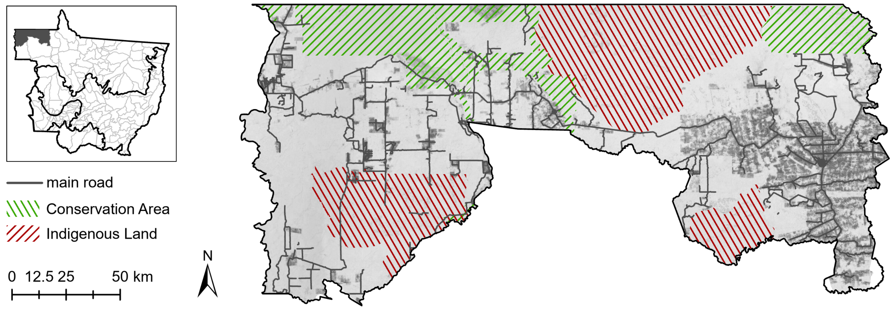
As basis for the fragmentation analysis, the municipality of Colniza was chosen to exemplify different forest fragmentation patterns (Figure 2). Colniza is located in the northwestern part of Mato Grosso within the Amazon biome, on the border to the state of Amazonas and covers an area of around 28,000 km${}^2$ [57]. Five conservation units as well as three indigenous lands are located in this municipality [47]. From an ecological perspective, Colniza is one of the few municipalities in the state with more than 90% of its forested area still preserved in 2004 [58]. Visual inspections of deforestation patterns from satellite imagery show that fishbone fragmentation is predominant, with rectangular patterns also present in some cases.

2.2. Data

For this study, atmospherically corrected surface reflectance from Landsat 5 TM and Landsat 8 OLI/TIRS time series data are used. The data are delivered together with a QA band (quality assessment band) indicating the presence of clouds [59]. Landsat 5 TM was launched on 1 March 1984 and was decommissioned on 5 June 2013. Landsat 8 OLI/TIRS was launched on 11 February 2013 and is still active [59]. Together, they cover a time span of 37 years with a revisit time of 16 days. In 2000 and 2001, a sensor error from Landsat 5 TM was identified over parts of the study area, which affects most of the period in which the annual mosaics are created. For this reason, these two years were not taken into account in all further evaluations. Likewise, change detection for the year 2002 (considering year${}_{2001}$ and year${}_{2002}$) are also affected and therefore not presented. In total, 11,144 scenes from Landsat 5 TM and 5643 scenes from Landsat 8 OLI/TIRS were processed.

The Landsat legacy is particularly suitable for tropical forest monitoring: Due to the medium spatial resolution of 30 m, even smaller-scale natural events and human interventions in forest areas can be detected. In addition, Landsat is the only freely available satellite image archive covering a period of more than three decades of earth observation at this spatial resolution, which allows a long retrospective analysis of land surface changes. In the future, the continuity of Landsat recordings will enable consistent observations [60].

For the accuracy assessment, the classifications created in this work are evaluated against the annual classifications of the Program for Monitoring Deforestation in the Brazilian Amazon (PRODES) with a minimum mapping unit of 6.25 ha, accessible via the National Institute for Space Research (INPE: http://www.obt.inpe.br/OBT/assuntos/programas/amazonia/prodes, accessed on 6 May 2021). The PRODES year of deforestation refers to the period from 1 August of one year to 31 July of the following year, e.g., annual deforestation for the year 2020 is obtained for the period of 1 August 2019 through 31 July 2020 [61]. However, only classifications from 2005 to 2019 are freely available and therefore used for the accuracy assessment. The datasets contain the four classes Forest, Non-Forest, Water, and Cloud. Other forest change dynamics such as forest degradation are not covered.

2.3. Preprocessing

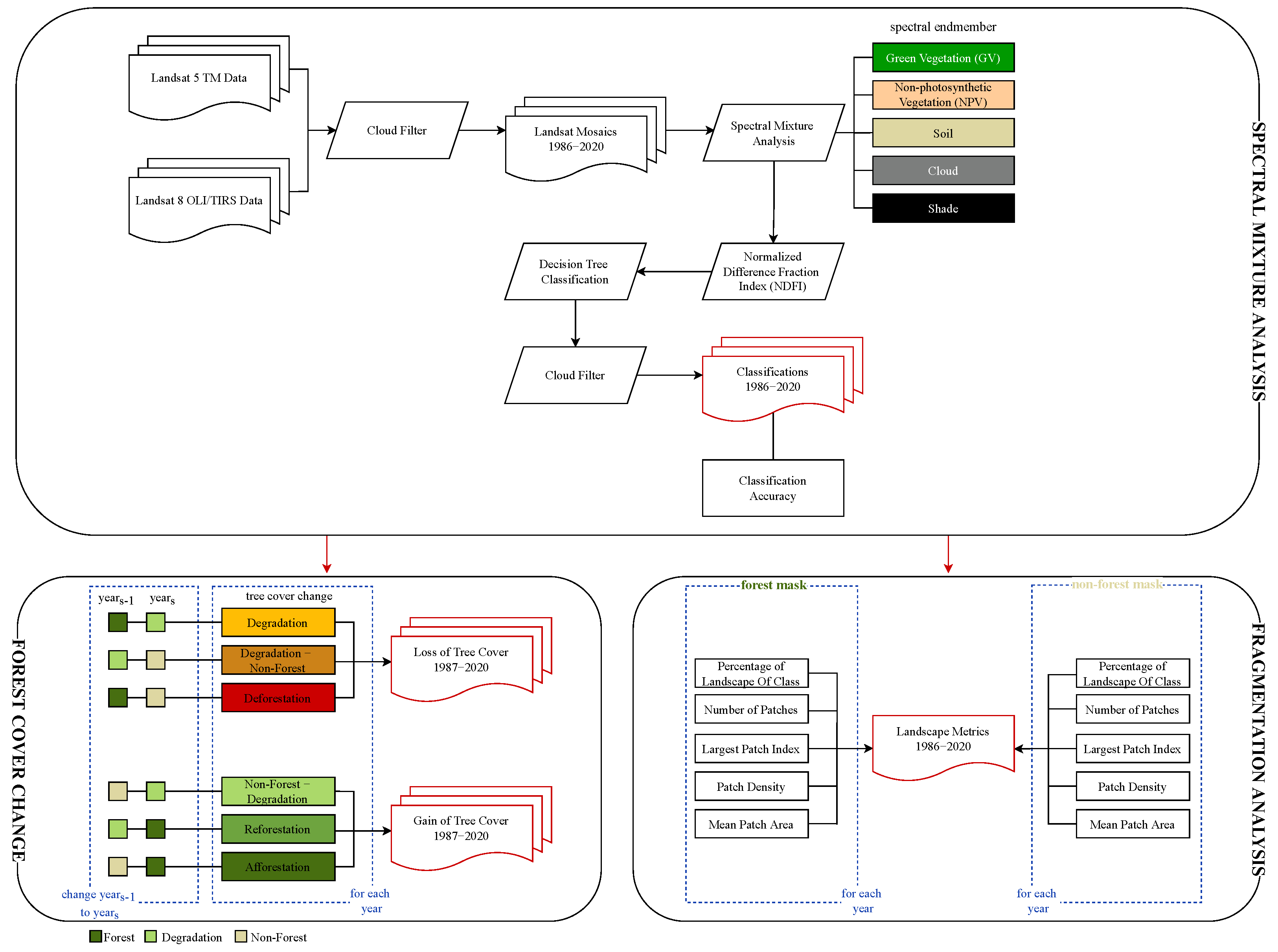
The approach of this work consists of several steps, schematically shown in Figure 3. In a first preprocessing step, annual multitemporal composite mosaics are built for the period between 1986 and 2020 based on the available imagery. Second, a cloud masking is performed. This is crucial because the study area is prone to a high cloud coverage due to the strong influence of the South Atlantic Convergence Zone (SACZ) [62]. The delivered QA band provides bitmasks for clouds and cloud shadows. All pixels containing the respective bit value are removed.

Furthermore, only images between the months of January and September are considered, since the dry season lasts until September in nondrought years, i.e., there are less clouds [49]. In addition, we target the months with high rates of slash-and-burn activities, which are between July and September in the Brazilian Amazon [63]. The annual composites are then created using the principle that the most recent and cloud-free pixel of all filtered scenes is used.

2.4. Spectral Mixture Analysis

2.4.1. Spectral Mixture Derivation

To detect forest degradation by selective logging or forest fires, a spectral mixture analysis (SMA) is applied in Google Earth Engine (GEE), which is described for the first time by Adams (1993) [64]. Thereby, the reflectance values per pixel are decomposed into different constituent spectra of pure materials, the so-called spectral endmembers, and corresponding fractions that correlate linearly with each other. The SMA obtains layers containing the pixelwise fraction for each specified endmember [21,22,65]. Thus, the resulting unmixing of pixels highlights details in subpixels and thereby possibly provides better results than conventional classification methods [65,66]. Spectral endmembers are often related to real-world objects in the study area, such as soil, water, metal, or any other natural or man-made material [65]. The selection of these endmembers is crucial for a representative SMA, since they have to reflect all ground materials present in the study area [30].

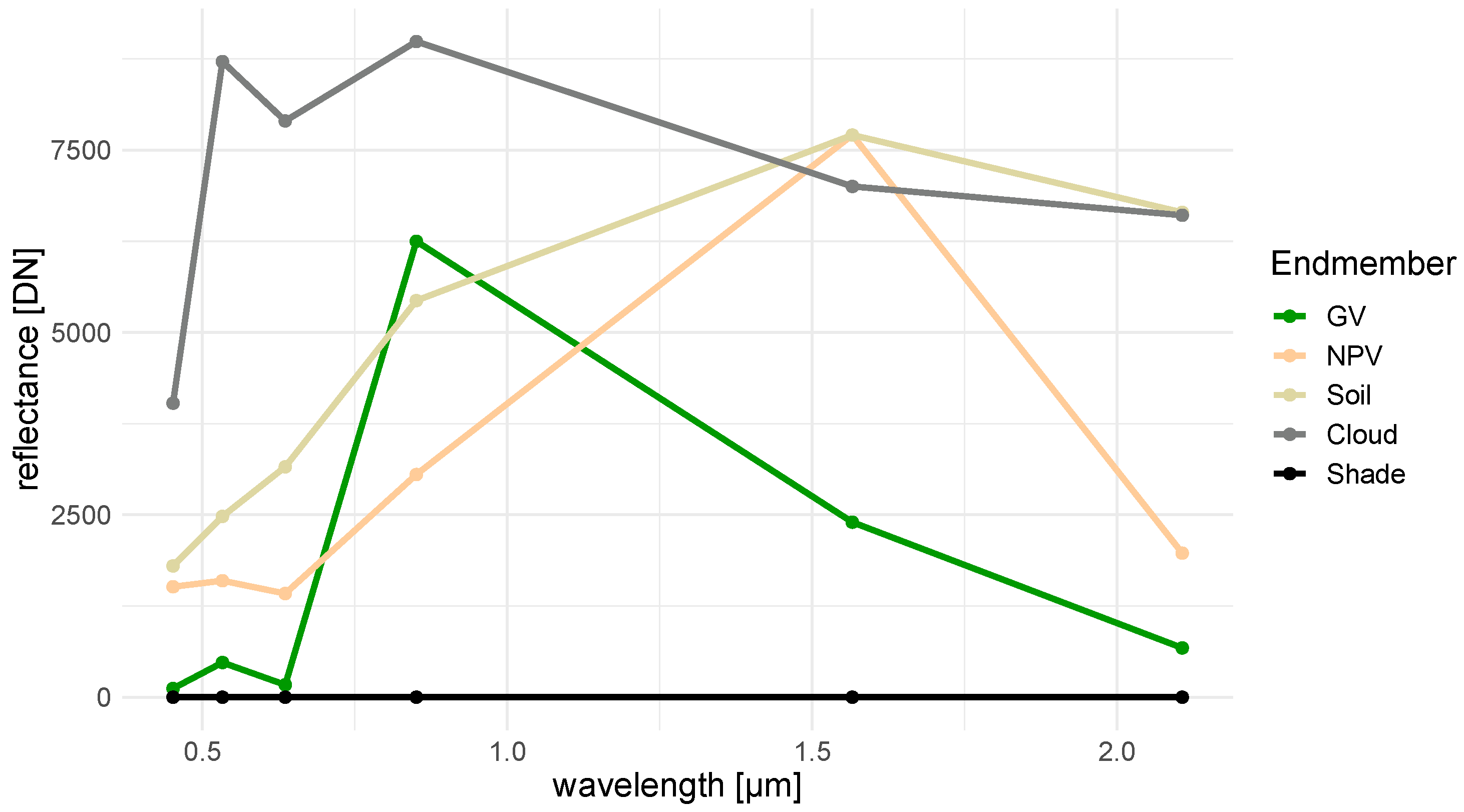
The defined endmembers in this study are Green Vegetation (GV), Non-photosynthetic Vegetation (NPV) (senescent vegetation, like dead trees or bark), Soil, and Shade, whereby the Landsat bands Blue, Green, Red, Near Infrared (NIR), Shortwave Infrared (SWIR) 1, and SWIR 2 were used for creating the spectral endmember curves. A fifth endmember, Cloud, was added afterward to capture clouds that were not detected by the initial masking [21]. The used endmember values in this study are derived by the Institute of People and the Environment of the Amazon (Imazon) [67] within the MapBiomas project (https://github.com/mapbiomas-brazil/amazon/blob/master/modules/SMA_NDFI.py, accesssed on 6 May 2021). This was done using 35,000 samples for the entire Amazon region from the reference database of the Laboratory of Image and Geoprocessing (LAPIG) of the Federal University of Goiás (UFG), trained and validated based on a random forest approach [68,69].

Figure 4 illustrates the reflection curves per endmember. GV shows the typical spectral profile for photosynthetically active vegetation, where reflectance sharply rises between the Red and NIR band, the so-called red edge. The shape of the Soil endmember curve increases with increasing wavelength because of iron oxide absorptions at shorter wavelengths. The NPV curve has tendencies of the GV curve (red edge characteristic), as well as of the soil reflectance curve. The reflectance value in the Red band is higher because of the degradation of chlorophyll pigments [70].

The SMA is based on Equation (1), where the reflectance of a given pixel ${\mathit{R}}_{\mathit{b}}$ in band $\mathit{b}$ is modeled as the sum of the reflectance of each endmember within a pixel multiplied by its fractional cover [64,71,72,73]:

$$\begin{array}{c}\hfill R_b=\sum _{i=1}^n{F}_i·R_{i,b}+{\epsilon }_b\end{array}$$

(1)

where

• ${\mathit{F}}_{\mathit{i}}$ is the fraction of endmember $\mathit{i}$ and
• $\mathit{n}$ is the number of pure spectra (endmembers).
• Unmodeled portions of the spectrum are expressed as residual error ${\epsilon }_b$ in band $\mathit{b}$.

All endmember fractions should sum to 1 and have positive values [74,75]. However, since the endmember Cloud was additionally added in this study, all endmembers add up to 1 plus the portion of the Cloud endmember fraction.

The SMA is applied to the Landsat mosaics throughout the obervation period.

Based on the fraction images resulting from the SMA, the Normalized Difference Fraction Index (NDFI), developed by Souza, Roberts, et al. (2005) [23], is calculated. The NDFI enhances the degradation signal resulting from selective logging or burning and is computed by:

$$\begin{array}{c}\hfill NDFI=\frac{G{V}_{Shade}-(NPV+Soil)}{G{V}_{Shade}+NPV+Soil}\end{array}$$

(2)

where the GV${}_{Shade}$ fraction is given by

$$\begin{array}{c}\hfill G{V}_{Shade}=\frac{GV}{100-Shade}\end{array}$$

(3)

The NDFI values range from −1 to 1. For all further analyses, the NDFI values are rescaled to 0–200. Intact forests show high values (close to 1) due to the combination of high GV${}_{Shade}$ (high GV and canopy Shade) and low NPV and Soil values. In degraded forest regions, the NDFI value decreases as NPV and Soil fractions increase. The NDFI has therefore the potential to identify degraded forest areas; the degradation is caused by burning and selective logging [21,22].

2.4.2. Decision Tree Classification

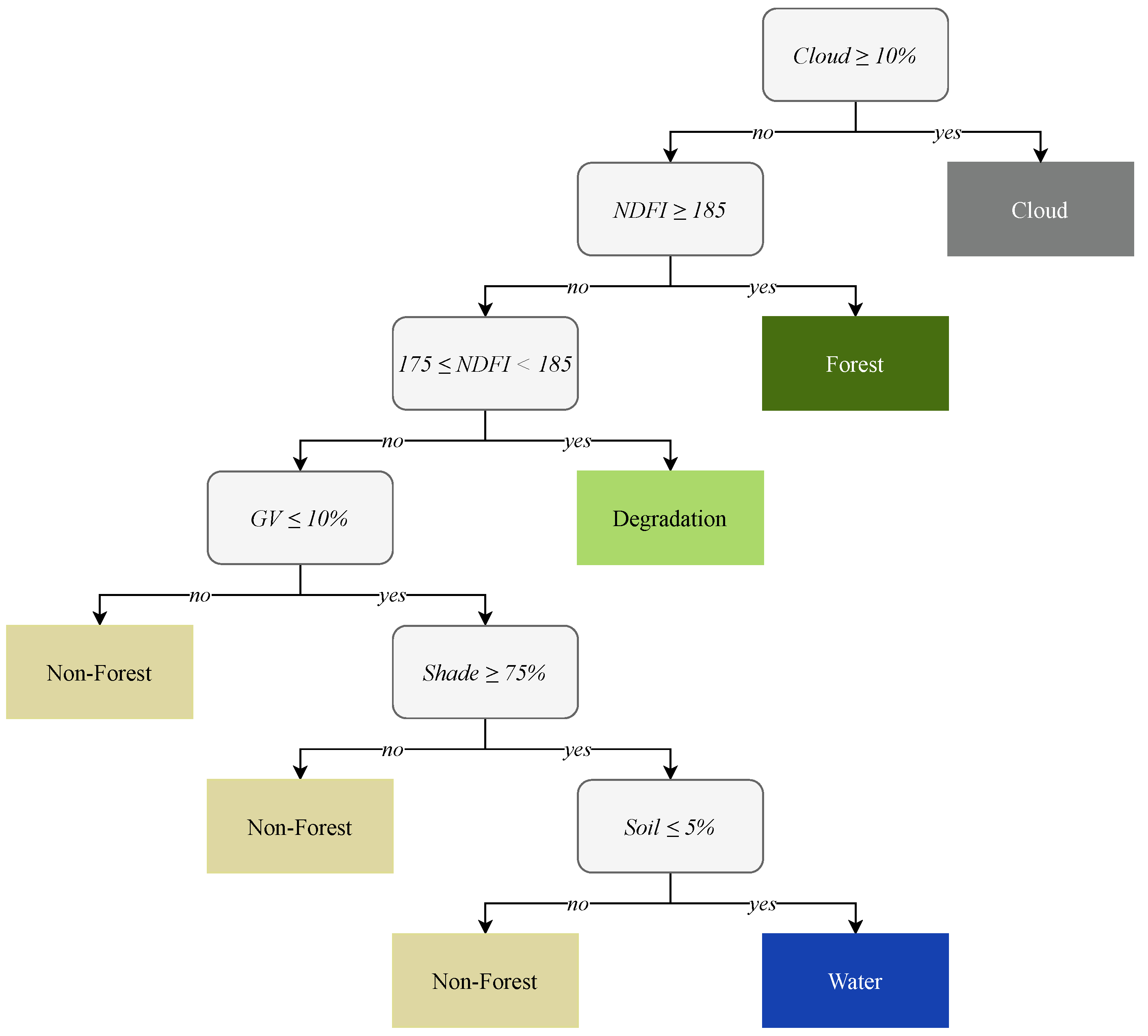
Based on the fraction images and the resulting NDFI, a decision tree classification (DTC) is carried out. The DTC threshold values were empirically derived by Souza and Siqueira (2013) [28] and Souza et al. (2013) [22] and adopted in this study since the thresholds had been developed for a research project in the Brazilian Amazon. Their hierarchical classification rules are based on image classification techniques in their custom-developed remote sensing data analysis software, training samples, and knowledge-based empirical algorithms [28]. For the classification in this study, five target classes are established: Forest, Degradation, Non-Forest, Water, and Cloud. Each of these classes is based on previously defined assumptions, shown in Figure 5: First, all cloudy pixels are masked, where endmember Cloud $\ge$10% is taken into account. All pixels that do not fulfill this condition will be used for all subsequent rules. For the DTC target classes Forest and Degradation the NDFI is utilized: pixels with NDFI $\ge$185 are assigned to the class Forest, pixels in the value range 175 $\le$ NDFI < 185 are assigned to the class Degradation. According to Souza and Siqueira (2013) [28], pixels belonging to the defined Degradation class represent areas of canopy damage larger than 25% caused by selective logging or forest fires. This is followed by the Water class, where endmembers GV and Soil show low fractions (GV $\le$10% and Soil $\le$5%), but high Shade fractions ($\ge$75%). If none of the conditions matches to a pixel, it will be assigned to the class Non-Forest.

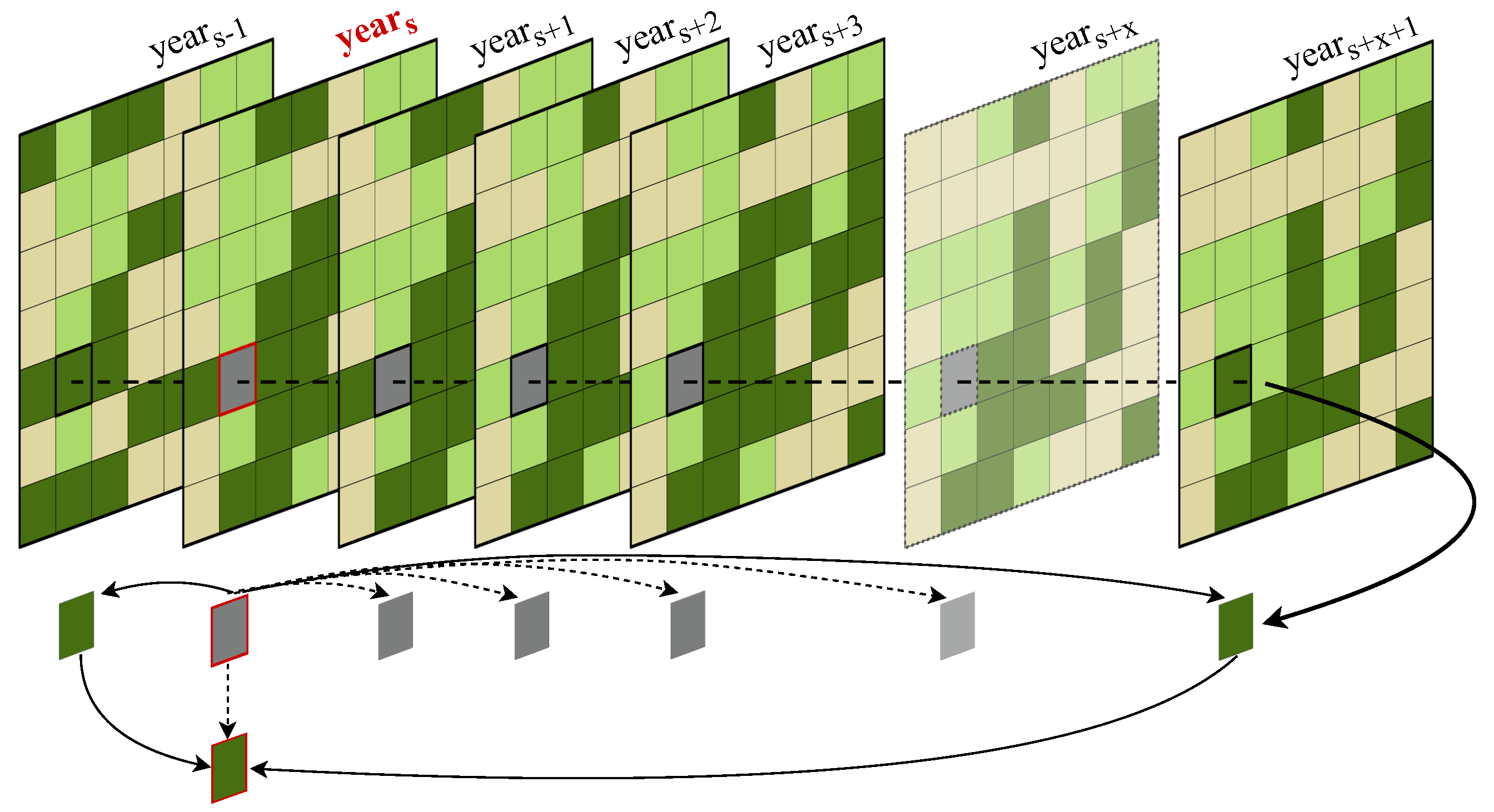
A cloud filter is applied after the DTC. Each pixel, classified as Cloud in the current Year${}_s$, is compared with the same pixel of Year${}_{s-1}$ and the following years (Year${}_{s+x}$).

According to Liebsch et al. (2008) [76] and Rozendaal et al. (2019) [77], a forest needs several hundred years to fully recover after clearing. Therefore, it can be ruled out that forest degrades and returns to its original canopy cover within a period of a few years. Similarly, degraded forest does not densify and noticeably degrade again within a short period of time or disappears entirely and then grows rapidly again. It can therefore be assumed that cloud pixels in the whole analysis period can be replaced by the class as which it was classified both in the year before the first cloud pixel (Year${}_{s-1}$) and in the year after the last successive cloud pixel (Year${}_{s+x+1}$). This means, for example, that if a pixel was classified as Forest in Year${}_{2006}$ and Year${}_{2010}$, but as Cloud in Year${}_{2007}$, Year${}_{2008}$ and Year${}_{2009}$, these three cloud pixels can be replaced by the class Forest. Figure 6 shows a schematic representation of this principle.

Since water bodies in the tropics are subject to high rates of hydrological dynamics, this rule is partially incorrect for the Water class. At the same time, water bodies certainly do not change from water to degraded or dense forest within a few years. Yet, the Water class plays a minor role in this study, as Forest, Degradation, and Non-Forest classes are of primary importance.

2.4.3. Acccuracy Assessment and Plausibility Analysis

For the accuracy assessment, the classifications created in this work are evaluated against the annual classifications of the PRODES dataset. Since the Cloud class, which is included in both classifications, would negatively affect the accuracy assessment and actually does not represent any data values, all cloud pixels in any of the classification (PRODES or classification of this study) were merged and masked out and not included in the accuracy assessment. Consequently, both classifications have the same cloud pixels, which are subsequently replaced by no data values. For the accuracy evaluation, 500,000 stratified random points were selected within each PRODES dataset, i.e., the number of pixels is proportionally distributed across the classes and afterwards compared with the corresponding pixel values of the classification performed in this study.

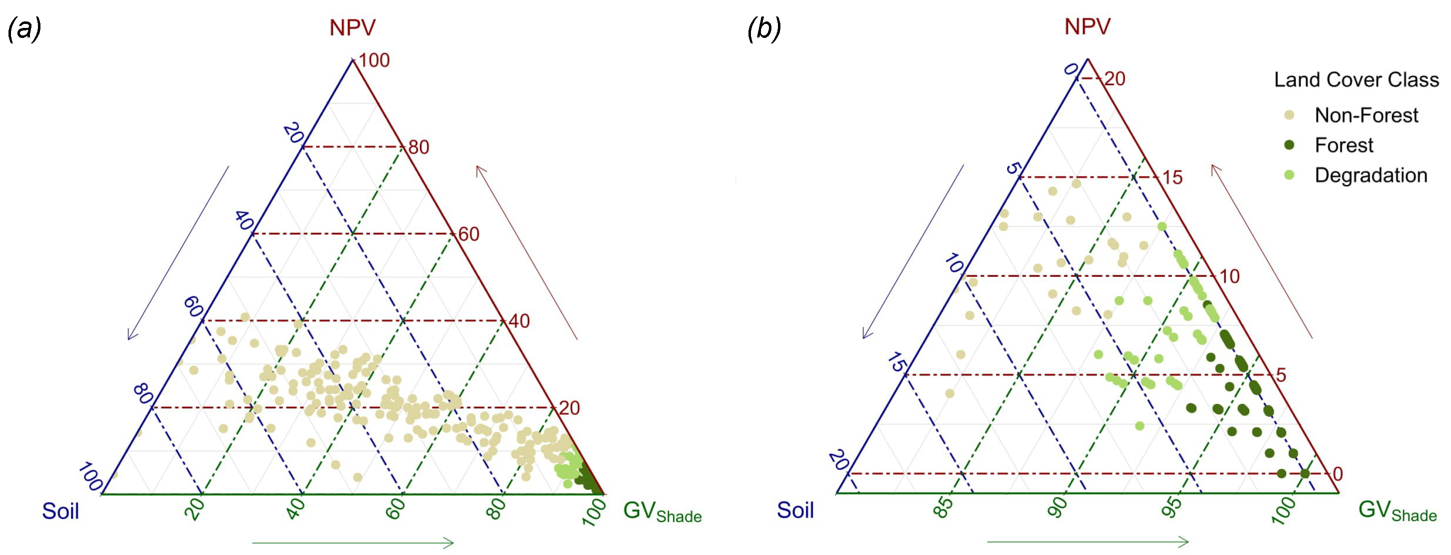
Since the classification of this study also includes the class Degradation, which is not listed in the PRODES dataset, a plausibility analysis of the class Degradation is performed as an additional step. For this purpose, a forest area in eastern Mato Grosso that changes over time was selected. 125 points were then randomly placed within this area for the years 1990, 2002, 2010, and 2020. This results in a total number of 500 pixels over the four selected years. From these pixels, the pixel values of the corresponding classifications were extracted, as were the respective pixel values of the NPV, Soil, and GV${}_{Shade}$ endmember bands. These selected three endmembers are critical for assigning the Landsat pixels to the Forest, Degradation, or Non-Forest classes in the DTC, as they are used in the NDFI (see Figure 5 and Equation (2)). Subsequently, only pixels corresponding to either the Non-Forest, Degradation, or Forest class are retained, resulting in 494 validation pixels.

2.5. Estimation of Forest Cover Change and Degradation

Annual rates of tree cover change are determined by implementing an additional new classification scheme based on the DTC results, consisting of six newly defined change classes, in which tree cover is lost or gained (see Figure 3). The classes Non-Forest, Degradation, and Forest from the DTC target classes are used for the reclassification. For the following analyses, it is disregarded whether the deforestation is of anthropogenic origin or natural. The aim is merely to analyze how the forest areas in Mato Grosso have changed between 1987 and 2020.

Tree cover loss is represented in three change classes: Pixels that were classified as Forest in Year${}_{s-1}$ and as Degradation in Year${}_s$ in the DTC are assigned to the new change class Degradation in Year${}_s$. Pixels that were classified as Degradation in Year${}_{s-1}$ and as Non-Forest in Year${}_s$ are reclassified to the new Degradation- Non-Forest class in Year${}_s$. The third class, Deforestation in Year${}_s$, contains all pixels that were detected as Forest in Year${}_{s-1}$ and Non-Forest in Year${}_s$.

Positive tree cover changes are reclassified as new Non-Forest-Degradation class in Year${}_s$, if Non-Forest pixels in Year${}_{s-1}$ change to Degradation in Year${}_s$. Pixels that were classified as Degradation in Year${}_{s-1}$ and as Forest in Year${}_s$ are reclassified as Reforestation in Year${}_s$. Non-Forest pixels in Year${}_{s-1}$ that changed to Forest in Year${}_s$ are reclassified as Afforestation in Year${}_s$.

Since a comparison is always made between the observed Year${}_s$ and the antecedent Year${}_{s-1}$, tree cover changes can only be detected from 1987 onward, as the first classification from 1986 does not precede any year included in this work.

2.6. Fragmentation Analysis

Fragmentation analyses are designed to study given landscapes and to quantify their changes over time [78]. In this context, landscape metrics are used to investigate and understand the structure, complexity and changes of certain landscapes in more detail [79]. To quantify the fragmentation level and the resulting composition and configuration of the forested and nonforested landscape in the selected municipality of Colniza, five landscape metrics were computed and are described in more detail in

Table 1. Used landscape metrics in this study (adapted from [80,81]).

Landscape metric	Equation	Unit	Short Description
Percentage of Landscape of Class ${\displaystyle PLAND}$	${\displaystyle PLAND=\frac{{\sum }_{j=1}^n{a}_{ij}}{A}\ast 100}$ ${\displaystyle a_{ij}}$ = area of each patch ${\displaystyle A}$ = total landscape area	percent [%]	Percentage of landscape belonging to class i. Describes the composition of the landscape.
Number of Patches ${\displaystyle NP}$	${\displaystyle NP=n_i}$ ${\displaystyle n_i}$ = number of patches	-	Number of patches of class i. Describes the fragmentation of the landscape.
Largest Patch Index ${\displaystyle LPI}$	${\displaystyle LPI=\frac{max{\left(a_{ij}\right)}_{j=1}^n}{A}\ast 100}$ ${\displaystyle max\left(a_{ij}\right)}$ = area of the largest patch ${\displaystyle A}$ = total landscape area	percent [%]	The proportion of total class comprised by the largest patch of class i. Simple measure of dominance.
Patch Density ${\displaystyle PD}$	${\displaystyle PD=\frac{n_i}{A}}$ ${\displaystyle n_i}$ = number of patches ${\displaystyle A}$ = total landscape area	[1/ha]	Density of patches of class i. Describes the fragmentation of the landscape.
Mean Patch Area ${\displaystyle ARE{A}_{MN}}$	${\displaystyle ARE{A}_{MN}=mean\left(AREA\left[patc{h}_{ij}\right]\right)}$ ${\displaystyle AREA\left[patc{h}_{ij}\right]}$ = area of each patch	hectare [ha]	Mean of all  patch areas belonging to class i. Describes the composition of the landscape.

using the Python package PyLandStats, developed by [80]. We aim to analyze how forest area in this community has changed between 1986 and 2020, without focusing on the cause of forest loss, i.e., anthropogenic or natural. To execute the selected landscape metrics, a forest mask is generated from each previously created land classification, as described in Section 2.4.1, which is then used as the input landscape. In addition, a nonforest mask is created for each classified year to be able to draw conclusions about landscape changes based on the analyzed forest fragmentation (Figure 3).

3. Results

3.1. Overall Classification Performance

Results show that the overall classification accuracy using the PRODES dataset for the years 2005 to 2019 is 85.6% and the average Kappa value 71.0%. The lowest Kappa value is 67.2% in 2012, the highest is 77.4% in 2007 (

Table 2. Overall accuracies and Kappa values for classifications from 2005 to 2019.

	2005	2006	2007	2008	2009	2010	2011	2012	2013	2014	2015	2016	2017	2018	2019	Mean
Overall Accuracy	0.859	0.859	0.890	0.859	0.846	0.871	0.859	0.834	0.854	0.845	0.852	0.846	0.853	0.853	0.858	0.856
Kappa	0.717	0.716	0.774	0.715	0.696	0.737	0.714	0.672	0.706	0.691	0.702	0.691	0.701	0.702	0.709	0.710

). According to Landis and Koch (1977) [82], Kappa values between 61.0% and 80.0% reflect a substantial strength of agreement. For the Forest class, the average producer’s accuracy is 90.3%, the user’s accuracy is 79.9%. The class Non-Forest has an average producer’s accuracy of 83.6% and a user’s accuracy of 96.3%.

The endmember fractions GV${}_{Shade}$, NPV, and Soil of the selected 494 points out of the Forest, Degradation, and Non-Forest classes for the plausibility analysis are shown in Figure 7. In Figure 7a, it can be seen that pixels assigned to the Non-Forest class show much higher intraclass variability than the two forest classes. In addition, the zoomed-in section in Figure 7b allows improved visual separation of degraded and forested pixels.

The following differences can be identified from the class statistics in

Table 3. Class statistics as used within the plausibility analysis, extracted from 494 random selected pixels.

Class	Fraction	Minimum (%)	Mean (%)	Maximum (%)	Standard Deviation
Non-Forest	NPV	0	11.2	20	4.4
	GV${\displaystyle {}_{Shade}}$	0	30.5	76	20.2
	Soil	0	18.6	53	10.3
Degradation	NPV	2	6.4	10	1.8
	GV${\displaystyle {}_{Shade}}$	70	77.1	83	3.0
	Soil	0	1.6	5	1.9
Forest	NPV	0	3.6	7	1.6
	GV${\displaystyle {}_{Shade}}$	75	88.3	100	9.3
	Soil	0	0.2	3	0.5

, calculated based on the points in Figure 7. The standard deviation of all displayed endmember fractions is highest for Non-Forest pixels. Furthermore, Forest pixels generally have lower scatter in NPV and Soil fractions than degraded pixels. Non-Forest pixels show the highest mean NPV fractions (mean = 11.2%), followed by degraded forest pixels (mean = 6.4%), whereas Forest pixels have the lowest mean value (mean = 3.6%). The opposite is true for the Soil fractions: Forest pixels show the lowest mean value (mean = 0.2%), Non-Forest pixels the highest (mean = 18.6%). Degraded pixel values are in between (mean = 1.6%) and much closer to Forest values. In addition, Forest pixels have the lowest standard deviation in the Soil fraction (sd = 0.5). A clear ascending mean value distribution is also visible in the GV${}_{Shade}$ fraction. Non-Forest pixels show the lowest mean GV${}_{Shade}$ value (mean = 30.5%), followed by Degradation (mean = 77.1%) and Forest (mean = 88.3%).

As explained in Section 2.4.1, degraded forests consist of mixed pixels, which include both soil and nonphotosynthetic vegetation in addition to green vegetation. The differences of the three classes just presented in Figure 7 confirm the assumption that degraded forest areas can be categorized as a separate class, since the NPV fraction lies between the values of Non-Forest (high NPV fraction) and Forest (low NPV fraction) pixels, although the transitions are smooth. This also testifies that degraded classified pixels cannot be assigned to Non-Forest, the value range for the Soil fractions differs by a great amount (Degradation: 0 ≤ Soil ≤ 5; Non-Forest: 0 ≤ Soil ≤ 53) (Table 3). Furthermore, the mean values of Degradation pixels of the GV${}_{Shade}$ fraction are closer to those of Forest than Non-Forest, indicating that degraded areas still contain significantly more green vegetation than nonforest areas. Nevertheless, the share in the GV${}_{Shade}$ fraction of Degradation pixels is always below 84%, on average at 77% and thus differs from Forest pixels. At the same time, the NPV fraction of the sample points of Degradation pixels is on average higher than that of Forest pixels, which together also indicates a separation of the classes Forest and Degradation.

3.2. Land Cover Change

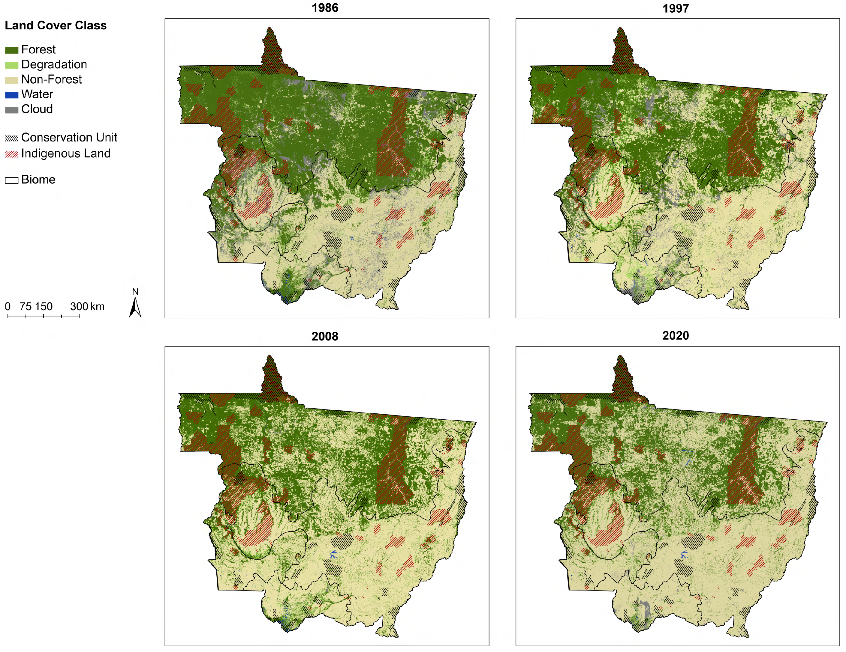
Using the classifications derived from the DTC, class distributions between 1986 and 2020 can be determined. Exemplary spatial visualization of land cover for the years 1986, 1997, 2008, and 2020 is given in Figure 8. In 1986, the forest cover in Mato Grosso comprises 48.7% and is reduced to 34.7% in 2020, representing a loss of more than 126,000 km${}^2$ over the entire analysis period. With increasing time, the southern forest boundary of the Amazon shifts northward until nonforest cover clearly predominates in 2020. Forest cover is also increasingly disappearing in the Pantanal. Comparing the forest cover from 1986 to 2020, it becomes clear that the remaining forest areas are mostly located in protected sites.

Areas classified as Non-Forest behave contrary to the Forest class. At the beginning of the time series, the Non-Forest share was 38.2% (1986) and reached 60.0% in 2020. The first time that the Non-Forest area is larger than the Forest area is in 1997, while the year before the shares were at similar levels with 43.7% Non-Forest and 44.3% Forest, respectively.

Despite increasing deforestation, the proportion of degraded areas remains almost constant (4.5% on average), with the lowest proportion of 2.9% in 2006 and the highest proportion of 6.0% in 1997. Degraded areas of the years shown have mostly disappeared in the subsequent visualized classification and have mainly passed into the class Non-Forest.

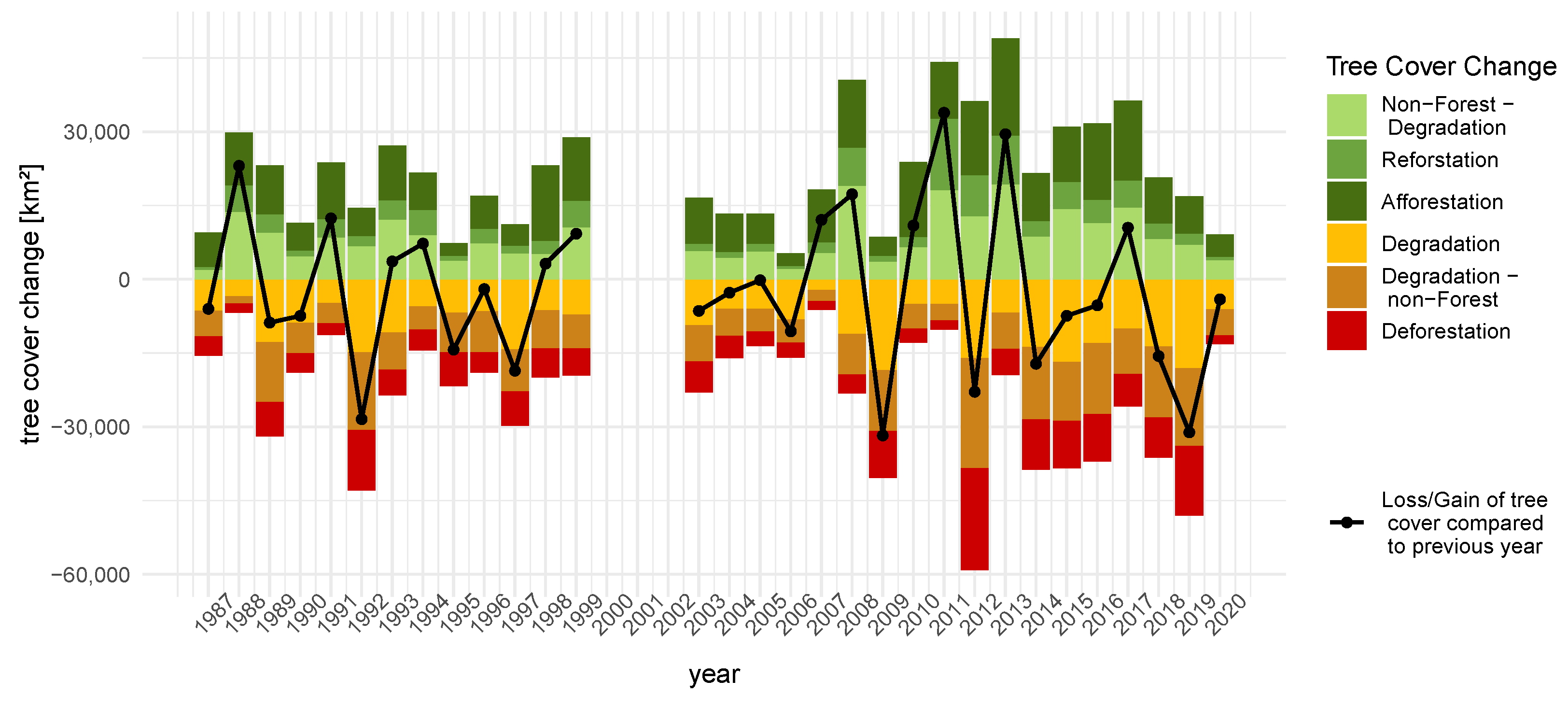
Derived from the classes Non-Forest, Degradation, and Forest from the DTC, tree cover changes per year, and the resulting annual loss or gain of tree coverage, calculated from the previous year’s values, is visualized in Figure 9. From this, 19 of 31 years analyzed experienced a negative trend where more tree cover is lost than gained (black line). Tree cover loss and gain fluctuates periodically in a two- to three-year cycle. Especially the years 1992, 2009, 2012, and 2019 experienced a strong loss of tree cover, between 23,000 km${}^2$ and 32,000 km${}^2$ compared to the previous year. Contrary to that, in 1988, 2011 and 2013, the gain in tree cover, compared to the other years, was highest, between 23,000 km${}^2$ and 34,000 km${}^2$.

The individual change classes provide deeper information on changes in tree cover. In general, the gain in tree cover shows a negative trend in recent years, but the loss shows a positive tendency and thus more tree cover is disappearing.

Gain in tree cover due to densification of degraded forest areas (Reforestation) has the smallest positive proportion in all years. Further positive tree cover changes, visualized as Afforestation and Non-Forest—Degradation classes, often show similar tree cover gains. The largest increase in trees is experienced in the year 2013 with a total of around 48,000 km${}^2$.

Per year, tree cover reductions are relatively evenly distributed within the three loss classes. The years 2012 and 2019 show a particularly high loss of tree cover in all three loss classes, with about 59,000 km${}^2$ and 48,000km${}^2$, respectively. The total amount of deforested areas, which was the smallest in 2007 with about 1800 km${}^2$ (about 2% of the state area of Mato Grosso), increased to its maximum in 2012 with almost 21,000 km${}^2$ (23% of the total area of Mato Grosso). The 70% increase in deforestation in 2019 compared to 2018 is particularly noticeable. Annual rates of areas affected by forest degradation are higher than deforestation rates for the entire period, except for 1995 and 2012, when deforestation rates were 2% and 23% greater, respectively. Forest changes by degradation were the highest with about 18,000 km${}^2$ in 2009, the lowest in 2007 with about 2000 km${}^2$.

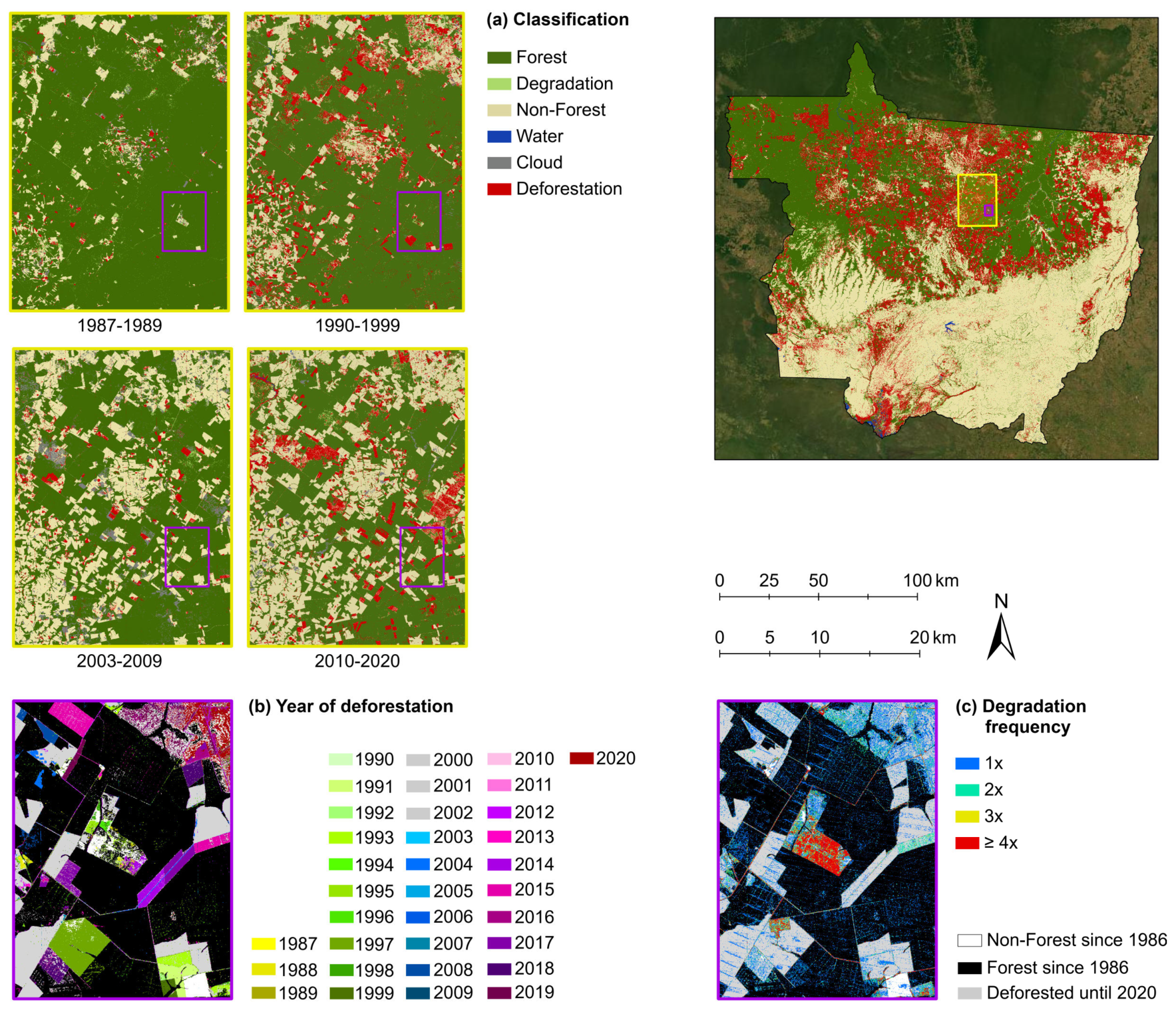
On the basis of annually deforested areas, temporal intensities of deforestation can also be mapped. Figure 10a shows this as an example for an area in the Amazon. The four sections show deforested areas, grouped in decades, where the last classification per analysis period is shown underneath. It is visible that the forest area was particularly present in the beginning of the analysis period. Over time, small areas, adjacent to already cut-down areas, are predominantly cleared, often with additional deforestation along road axes. In 2020, most of the forest has been cleared and nonforest areas dominate.

Figure 10b illustrates the year of deforestation for a selected part of the area in Figure 10a. Cleared areas, visualized in grey, cannot be assigned to a specific year, rather the interval between 2000 and 2002, due to the sensor error in 2000 and 2001. The areas in the Southeast show that areas there were cleared in the 1990s and now result in one large unwooded patch. Areas for the creation of roads were also cleared in different years. Following the new road course of 2004 in the eastern part, newly cleared areas of different years in the 2010s are adjacent on both road sides.

The same site from Figure 10b is also shown in Figure 10c. This map refers to the degradation frequency over the period from 1986 to 2020. Degraded areas of the same frequency often occur in patterns, for example, along logged roads as well as on later or previously cleared areas. It is noticeable that they reflect the spatial limitations and patterns of the deforested areas. The area to the East (turquoise), which has been degraded at least two times, is as densely degraded and has similar dimensions as the area deforested in 2013 in Figure 10b. The same can be observed for the large northeastern area. It is degraded with the same patchiness as the corresponding deforested site in Figure 10b.

3.3. Forest Fragmentation

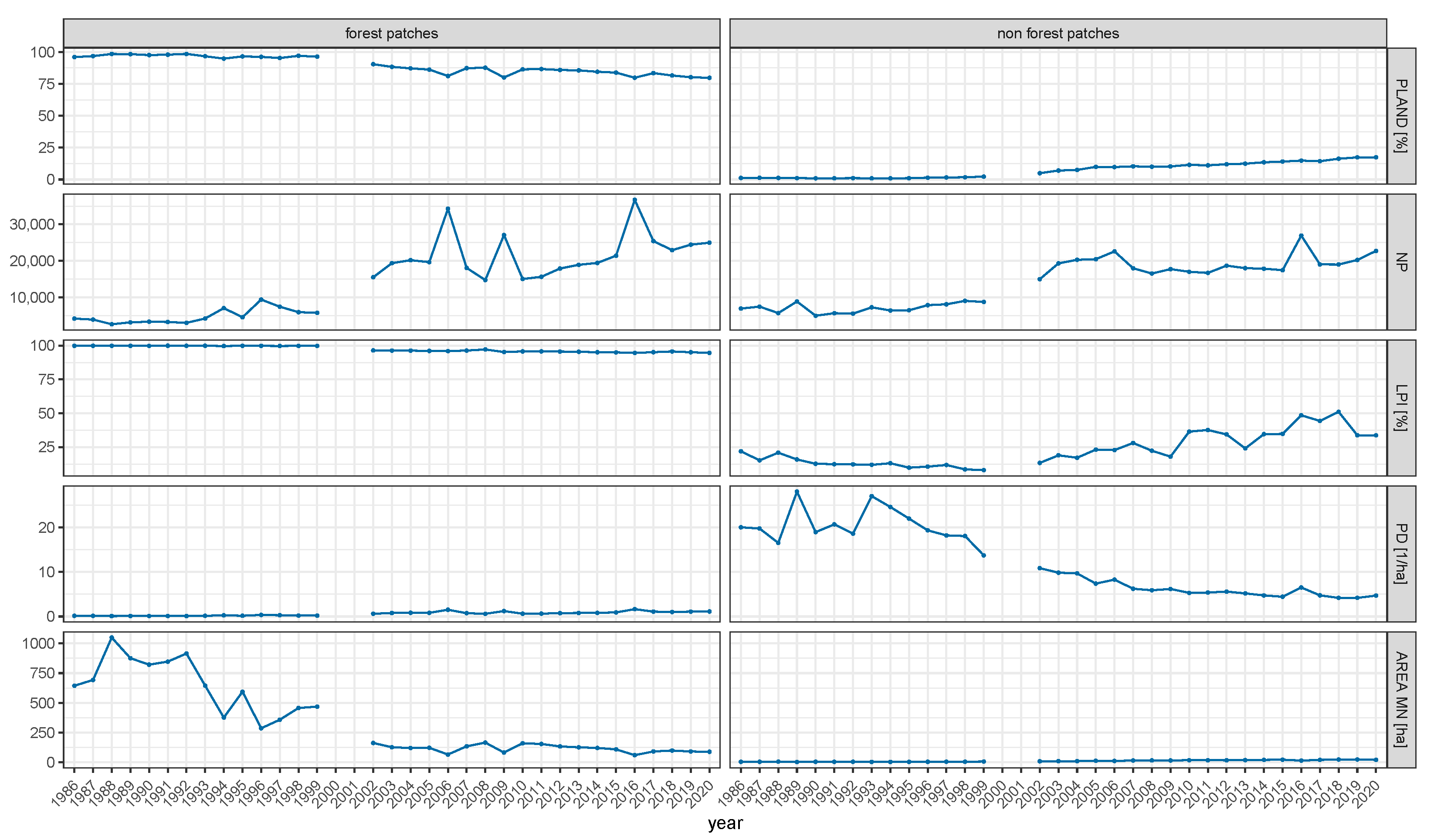
The results of the five processed landscape metrics for the municipality of Colniza are shown in Figure 11. This plot includes a combination of the distribution of the calculated landscape metric values and the change of these over time.

At the beginning of the time series, the forest area comprises nearly 100% (PLAND index). The forest area decreases over time, although it remains above 75% in 2020. Converging to this, the PLAND index increases over time in nonforested areas.

Value distribution of the number of forest patches (NP) varies to a greater extent. More and more forest fragments are created over time. Until 1999, this number is below 10,000; afterward, the number increases and doubles to about 20,000 in 2004. With approximately 34,300 patches, the peak is reached in 2016. Similarly, the number of nonforested areas is increasing over the years.

The largest forest area (LPI) in Colniza remains stable containing over 94% of the total forest area. However, there is a slight downward trend through the years. The LPI of the nonforested areas differs strongly from forested areas. At the beginning of the time series, LPI values are smaller than 25%. Until 2006, values remain below 25%, mostly even below 15%, before increasing up to 50%.

Patch density (PD) in forested areas increases over the years but remains between 0.1 and 1.8 patches/ha throughout the analysis period, with values mostly below 1 patch/ha. In contrast, patch density in nonforested areas decreases steadily from an initial rate of almost 28 patches/ha to about 5 patches/ha in 2020. From 2006, patch density already averages about 6 patches/ha.

The results of AREA${}_{MN}$ in forested areas change significantly. Forest fragments are largest at the beginning of the analysis period (1049 ha in 1988) and decrease continuously until 1999 (468 ha). A subsequent abrupt loss of area per patch to below 250 ha can be observed, reaching its smallest area of 61 ha in 2016.

Hence, it can be summarized that the forest area and largest forest patch are not only decreasing over time, but due to the increasing NP and PD and decreasing AREA${}_{MN}$, the forested landscape becomes more and more fragmented.

Subsequent to these statistical observations, further insights into fragmentation patterns can be obtained. In the first couple of years the percentage of the largest forested patch in the municipality of Colniza changes only slightly, suggesting that contiguous forest areas are not completely separated by deforestation but only incised. This assumption is also supported by the increasing percentage of LPI for unforested patches. Consequently, the largest unwooded patch has probably increased in size over the years as smaller patches were connected by logging of intervening forested areas. Similarly, it is apparent that a break point occurs in 2002. Not only does the average forested patch area decrease by more than 50% from this point, but the number of forest patches almost triples compared to the previous computed year. As the NP of forested land increases, so does the number of patches of nonforested land. A reason could be the effect that the more forest is cleared, the more nonforested patches are created and thus increasing the number of unconnected forest patches.

Changing logging patterns as of 2002 may be one reason for this progression, as it is shown in Figure 12. Until 1999, the predominant logging pattern is marked by the fishbone fragmentation. Especially in the eastern part of the municipality, this logging technique is used (see Section 2.1). At this time, forest patches were logged only sporadically on a small scale and new cutting is predominantly adjacent to existing roads (Figure 12b). As a result, few new patches are created, most of the forest area remains contiguous, and the total forest area decreases only slightly. Due to this method, the PD of deforested areas per hectare is high. However, starting in 2002, many large rectangular, widely distributed, and noncontiguous patches were also increasingly cleared in the West of the municipality, which may explain the high forest loss and decrease in patch density of nonforested areas in Colniza starting that year. This new logging pattern leads to the construction of more and more new roads in the West (see Figure 12a, new road since 2002 in the southwestern part of the map) through previously contiguous forest or protected areas, creating new forest and unforested patches. In addition, the rate of logging in the East of the region is increasing tremendously in the original fishbone fragmentation area (Figure 12b), which in turn is causing many small patches, increasing the number of forest/unforested patches, and decreasing the average forest area. In addition, the initially comparatively small unwooded patches are enlarged by clearing adjacent forests.

4. Discussion

4.1. Spectral Mixture Analysis and Fraction Image Classification

The main objective of this study was the application of a classification methodology for identifying forest and degraded forest areas to draw conclusions on temporal and spatial forest cover changes between 1987 and 2020 in Mato Grosso by using a subpixel analysis. In general, the demarcation of degraded forest to forest and nonforest is difficult due to the combination of different land cover types, such as vegetation, soil, or dead wood, which causes a mixed pixel problem [21]. This challenge could be solved through the SMA, where pixels are divided into individual fractions of previously specified endmembers, which allows them to be assigned to a certain class using a DTC. The success of an SMA highly depends on the accuracy of the spectral endmember’s selection, as they must reflect all ground materials [30]. Endmembers must be chosen in such a way that all ground entities are covered but spectrally differ from each other [83]. The accuracy of an SMA therefore depends on both the within-class variability and the between-class variability of the selected endmembers [84]. The higher the within-class variability, i.e., the variability within an endmember class, the lower the accuracy [84,85]. Likewise, spectrally similar endmembers lead to a high between-class variability and to false results [83,84]. Since Imazon (2019) [67] already defined meaningful endmembers through their expert knowledge within the MapBiomas project for the Amazon, these could be used for this work and meaningful results could be derived.

In order to classify the individual pixels with the help of fraction images, thresholds were defined per class. Previous studies showed that the determination and selection of thresholds used in DTCs can be locally applied to land cover classifications but cannot be adopted in other areas without taking the different vegetation types present there into account [86]. The thresholds of Souza and Siqueira (2013) [28] and Souza et al. (2013) [22], who carried out an SMA with a subsequent DTC in the same study area, could therefore be adopted but cannot be regarded as general rules. The results of the fraction image classification show a mean overall accuracy of 85.6% and a mean producer’s accuracy of 90.3% in mapping forest areas between 2005 and 2019 in Mato Grosso, which correspond well to studies attempting to classify land cover structures for the same study region [27,28,87]. Given that the minimum mapping unit of PRODES, the reference data set used for the accuracy assessment, is 6.25 ha, smaller land cover features are not considered in this dataset. This contributes to partially inaccurate results in the accuracy assessment performed, where mapped small-scale land cover changes of our study could not be considered and were recorded as misclassified.

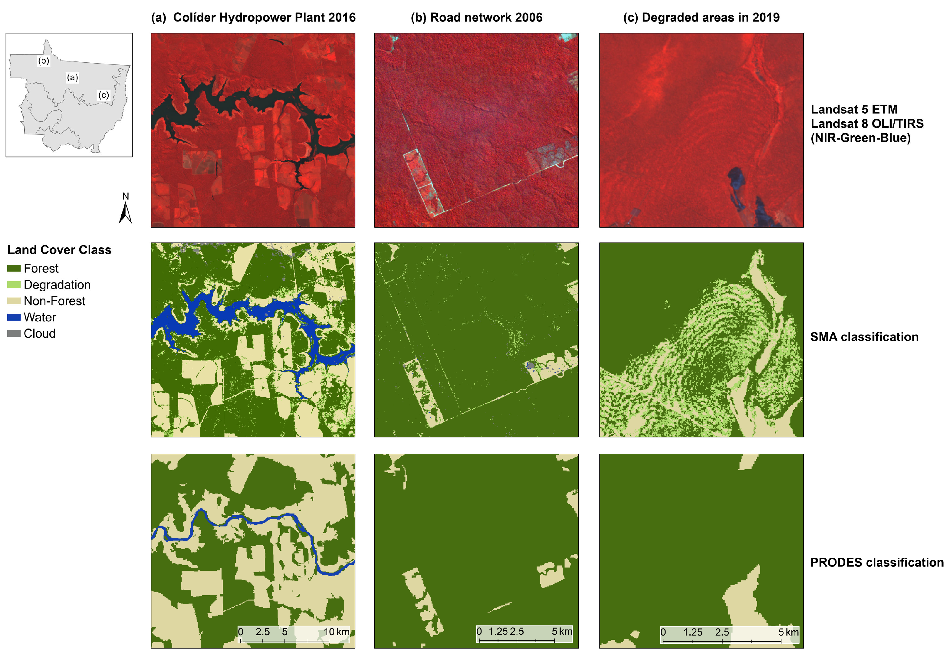
Further errors within the accuracy assessment may result from different time periods in the prediction and reference dataset. In addition, secondary forest regrowth and degraded forest areas are not recorded in PRODES [88]. Consequently, all areas classified as degraded in this study are represented with an accuracy of 0%. Likewise, woodlands in the Cerrado biome are mostly classified as nonforest [88]. It can thus be presumed that the accuracy of the classifications may be even higher than determined by the accuracy assessment. As Tyukavina et al. [88] also describe, the PRODES classifications are spatially not accurate and required manual improvements. Visual inspection also revealed misclassifications of water in this datasets. For example, the Colíder Hydropower Plant is not recorded until 2016 and only the original course of the river is visible (Figure 13a). Therefore, PRODES classifications might be examined more closely in analyses involving deforestation rates in the Brazilian rainforest.

Degraded forest areas in this study were evaluated with the help of a plausibility analysis and visual interpretation. This showed that distinguishing between degraded and intact forest using the NDFI and thresholds is certainly possible, where the required endmember fractions in these two classes can be separated from each other. Nevertheless, it is important to note that the separability of the degradation and forest classes applied here need to be verified by ground truth data to avoid possible erroneous assumptions.

4.2. Change Detection

The change detection analysis showed that forest area decreased by 28.8% between 1987 and 2020.

For the period assessed in this study, different deforestation rates are reported from other analyses or monitoring systems for the same study area. Comparing these different products is challanging because the results are based on various data and methods. For example, it is difficult to compare the deforestation rates collected in this study with the official products of the State of Brazil. As previously mentioned, the minimum mapping unit of deforestation rates determined by PRODES is 6.25 ha, which ignores smaller modified forest areas, but is well captured by the method in this work. Figure 13b shows this clearly: in the satellite image of 2006, narrow streets can be seen that were also captured by the SMA classification but were not recorded in the PRODES dataset of 2006. In addition, different class definitions play an important role. Since PRODES does not take into account degraded areas, these areas are included in other classes, for example, forest or nonforest, leading to erroneous assumptions in direct comparisons. Figure 13c clearly highlights these classification differences: while the SMA classification captured undulating deforested and degraded areas, the same extent is mapped as forested in the PRODES dataset. This difference in data could be the reason for a 62.9% lower deforestation rate between 2004 and 2019 in the PRODES dataset compared to this study. However, even more detailed research is needed to validate this assumption and clearly determine the discrepancies.

The type of forest loss was disregarded in this work, as the focus was on the change and not primarily on the reason for it. Further analyses could provide information on this, for example, whether forest has degraded or disappeared through anthropogenic intervention (manual logging or burning) or has been destroyed by natural factors (wind, wildfire, etc.).

In summary, it can be said that the presented method to determine forest degradation and deforestation can be an important tool to continue monitoring forest changes and to determine, for example, the performance of protected areas and land management measures that should aim to reduce deforestation and forest degradation and curb illegal deforestation.

4.3. Forest Fragmentation

Based on the landscape metrics performed, temporal changes in the landscape could be observed.

The largest patch (LPI) and average patch size (AREA${}_{MN}$) of forested land in Colniza decreased as deforestation increased. Similarly, patch density (PD) of unforested areas decreased with increasing deforestation through the years, with AREA${}_{MN}$ showing little change. The greatest variation is observed in the interannual variation of the number of forested and nonforested patches (NP).

The calculated landscape metrics could also be used to show impacts of different deforestation forms. The fishbone logging pattern in Colniza is especially prominent in decreasing AREA${}_{MN}$ of forest patches and PD of cleared areas. To support the assumption that different deforestation patterns lead to different results of certain landscape metrics, more areas with dominant deforestation patterns would need to be analyzed in terms of representative results.

The data basis is also essential. Due to the Landsat sensor resolution of 30 m, some small-scale changes, such as forest aisles or patches smaller than 90 m${}^2$ cannot be recorded, which can certainly distort the result. For example, patches that are perceived as separate in the classification might be connected in reality by a narrow forest strip and thus the actual number of patches would be smaller. Therefore, a data set with a higher spatial resolution could lead to different results. It should also be mentioned that due to the partionally incomplete eliminated cloud cover, cloudy forest or nonforest areas could not be considered in this analysis. If a forest area is partially covered with clouds in one year, the extracted forest mask delivers distorted results, for example, more patches or a smaller LPI are detected, although they are actually connected. If in the following year this forest patch is free of clouds, this area is included in the analysis and reflects the actual reality. While an in situ field survey would provide the most accurate data for determining individual patches and their potential connectivity, it is nearly impossible to realize it for such a large study area.

Apart from the methodical identification of forest fragmentation, it would certainly be interesting to determine its consequences for flora and fauna and to establish possible actions. Since forest edges represent habitats with different characteristics than forest interiors [90], the identification of edge and core forest could determine consequences for population dynamics or community structures, such as the increased predation from bird nests at forest edges [91].

In fact, there is disagreement among scientists about whether habitat fragmentation is good or bad for biodiversity (e.g., [35,92]), making the results of the fragmentation analysis from this work difficult to interpret. More studies would certainly have to be carried out, considering various factors. It can only be stated that large contiguous habitat patches should be preserved if fragmentation has predominantly negative effects on species diversity. If fragmentation has predominantly positive effects on species, then the focus should be on the preservation of a large number of small patches. In case fragmentation has neither negative nor positive effects on species diversity, the primary objective should be to protect all habitats, regardless of their size or distribution [92]. However, as shown in Section 3.3, it is not necessarily a matter of determining the best logging practice, but of the rapidity and intensity with which forests are disappearing and how this will affect any species in the future [39].

5. Conclusions and Outlook

This study analyzes the temporal and spatial effects of forest loss in Mato Grosso over 34 years. The availability of time series data from the Landsat legacy with high temporal and spatial resolution offers a cost-effective and solid basis for the analysis of interannual forest change. With this dataset, the complete analysis period in Mato Grosso could be covered. Additional cloud filters also help to reduce most of the cloud cover and thus improve the data basis. Nevertheless, the given resolution of 30 m can also be a limiting factor, since small-scale changes cannot be detected.

The fraction image classification provides a good technique to distinguish forest from nonforest and also degraded forest in the Amazon region. For the transferability of the used endmembers to other regions of interest, the ground materials must show the same spectral characteristics of the study area described here. Based on the classification, different processes of temporal forest cover change can be identified. In the majority of the analyzed years, forest loss is greater than gain, with irregular variation between years. To mitigate the resulting impacts in the future, it is important to continue the close monitoring of changes in the rainforest and to take further mandatory policy decisions, not least to achieve the goal of zero illegal deforestation in the Amazon by 2030 [93].

In order to measure altered forest structures in the community of Colniza, the conducted fragmentation analysis shows that different logging patterns result in different forms of fragmentation which are measured by landscape metrics. In general, the fragmentation of forest areas increases, resulting in changing habitats for flora and fauna. These results can help to better observe and analyze forested areas and to take appropriate decisions to protect this fragile ecosystem.

References

1. Simoes, R.; Picoli, M.C.A.; Camara, G.; Maciel, A.; Santos, L.; Andrade, P.R.; Sánchez, A.; Ferreira, K.; Carvalho, A. Land use and cover maps for Mato Grosso State in Brazil from 2001 to 2017. Sci. Data 2020, 7, 34. [Google Scholar] [CrossRef] [PubMed] [Green Version]
2. FAO. The State of Agricultural Commodity Markets 2018: Agricultural Trade, Climate Change and Food Security; FAO: Roma, Italy, 2018. [Google Scholar]
3. Picoli, M.C.A.; Rorato, A.; Leitão, P.; Camara, G.; Maciel, A.; Hostert, P.; Sanches, I.D. Impacts of Public and Private Sector Policies on Soybean and Pasture Expansion in Mato Grosso—Brazil from 2001 to 2017. Land 2020, 9, 20. [Google Scholar] [CrossRef] [Green Version]
4. Lapola, D.M.; Martinelli, L.A.; Peres, C.A.; Ometto, J.P.H.B.; Ferreira, M.E.; Nobre, C.A.; Aguiar, A.P.D.; Bustamante, M.M.C.; Cardoso, M.F.; Costa, M.H.; et al. Pervasive transition of the Brazilian land-use system. Nat. Clim. Chang. 2014, 4, 27–35. [Google Scholar] [CrossRef] [Green Version]
5. Beuchle, R.; Grecchi, R.C.; Shimabukuro, Y.E.; Seliger, R.; Eva, H.D.; Sano, E.; Achard, F. Land cover changes in the Brazilian Cerrado and Caatinga biomes from 1990 to 2010 based on a systematic remote sensing sampling approach. Appl. Geogr. 2015, 58, 116–127. [Google Scholar] [CrossRef]
6. Da Cruz, D.C.; Benayas, J.M.R.; Ferreira, G.C.; Santos, S.R.; Schwartz, G. An overview of forest loss and restoration in the Brazilian Amazon. New For. 2021, 52, 1–16. [Google Scholar] [CrossRef] [Green Version]
7. IBGE. Produção Agrícola Municipal—PAM: Séries históricas. Available online: https://www.ibge.gov.br/estatisticas/economicas/agricultura-e-pecuaria/9117-producao-agricola-municipal-culturas-temporarias-e-permanentes.html?=t=series-historicas (accessed on 10 March 2021).
8. Broadbent, E.N.; Asner, G.P.; Keller, M.; Knapp, D.E.; Oliveira, P.J.; Silva, J.N. Forest fragmentation and edge effects from deforestation and selective logging in the Brazilian Amazon. Biol. Conserv. 2008, 141, 1745–1757. [Google Scholar] [CrossRef]
9. De La Vega-Leinert, A.C.; Huber, C. The Down Side of Cross-Border Integration: The Case of Deforestation in the Brazilian Mato Grosso and Bolivian Santa Cruz Lowlands. Environ. Sci. Policy Sustain. Dev. 2019, 61, 31–44. [Google Scholar] [CrossRef]
10. Bullock, E.L.; Woodcock, C.E.; Souza, C.; Olofsson, P. Satellite-based estimates reveal widespread forest degradation in the Amazon. Global Chang. Biol. 2020, 26, 2956–2969. [Google Scholar] [CrossRef]
11. Nogueira, E.M.; Yanai, A.M.; de Vasconcelos, S.S.; de Alencastro Graça, P.M.L.; Fearnside, P.M. Brazil’s Amazonian protected areas as a bulwark against regional climate change. Reg. Environ. Chang. 2018, 18, 573–579. [Google Scholar] [CrossRef]
12. Cochrane, M.A. Fire science for rainforests. Nature 2003, 421, 913–919. [Google Scholar] [CrossRef]
13. Silvério, D.V.; Brando, P.M.; Bustamante, M.M.C.; Putz, F.E.; Marra, D.M.; Levick, S.R.; Trumbore, S.E. Fire, fragmentation, and windstorms: A recipe for tropical forest degradation. J. Ecol. 2019, 107, 656–667. [Google Scholar] [CrossRef]
14. Bustamante, M.M.C.; Roitman, I.; Aide, T.M.; Alencar, A.; Anderson, L.O.; Aragão, L.; Asner, G.P.; Barlow, J.; Berenguer, E.; Chambers, J.; et al. Toward an integrated monitoring framework to assess the effects of tropical forest degradation and recovery on carbon stocks and biodiversity. Global Chang. Biol. 2016, 22, 92–109. [Google Scholar] [CrossRef] [PubMed]
15. Dupont, S.; Brunet, Y. Impact of forest edge shape on tree stability: A large-eddy simulation study. Forestry 2008, 81, 299–315. [Google Scholar] [CrossRef] [Green Version]
16. Lovejoy, T.E.; Nobre, C. Amazon Tipping Point. Sci. Adv. 2018, 4, eaat2340. [Google Scholar] [CrossRef] [PubMed] [Green Version]
17. DeWalt, S.J.; Maliakal, S.K.; Denslow, J.S. Changes in vegetation structure and composition along a tropical forest chronosequence: Implications for wildlife. For. Ecol. Manag. 2003, 182, 139–151. [Google Scholar] [CrossRef]
18. Laurance, W.F.; Lovejoy, T.E.; Vasconcelos, H.L.; Bruna, E.M.; Didham, R.K.; Stouffer, P.C.; Gascon, C.; Bierregaard, R.O.; Laurance, S.G.; Sampaio, E. Ecosystem Decay of Amazonian Forest Fragments: A 22-Year Investigation. Conserv. Biol. 2002, 16, 605–618. [Google Scholar] [CrossRef] [Green Version]
19. Baccini, A.; Goetz, S.J.; Walker, W.S.; Laporte, N.T.; Sun, M.; Sulla-Menashe, D.; Hackler, J.; Beck, P.S.A.; Dubayah, R.; Friedl, M.A.; et al. Estimated carbon dioxide emissions from tropical deforestation improved by carbon-density maps. Nat. Clim. Chang. 2012, 2, 182–185. [Google Scholar] [CrossRef]
20. Esquivel-Muelbert, A.; Baker, T.R.; Dexter, K.G.; Lewis, S.L.; Brienen, R.J.W.; Feldpausch, T.R.; Lloyd, J.; Monteagudo-Mendoza, A.; Arroyo, L.; Álvarez-Dávila, E.; et al. Compositional response of Amazon forests to climate change. Global Chang. Biol. 2019, 25, 39–56. [Google Scholar] [CrossRef] [Green Version]
21. Achard, F.; Boschetti, L.; Brown, S.; Brady, M.; DeFries, R.; Grassi, G.; Herold, M.; Mollicone, D.; Mora, B.; Pandey, D.; et al. A Sourcebook of Methods and Procedures for Monitoring and Reporting Anthropogenic Greenhouse Gas Emissions and Removals Associated with Deforestation, Gains and Losses of Carbon Stocks in Forests Remaining Forests, and Forestation; Wageningen University: Wageningen, The Netherlands, 2014. [Google Scholar]
22. Souza, C.M.; Siqueira, J.; Sales, M.; Fonseca, A.; Ribeiro, J.; Numata, I.; Cochrane, M.; Barber, C.; Roberts, D.; Barlow, J. Ten-Year Landsat Classification of Deforestation and Forest Degradation in the Brazilian Amazon. Remote Sens. 2013, 5, 5493–5513. [Google Scholar] [CrossRef] [Green Version]
23. Souza, C.M.; Roberts, D.A.; Cochrane, M.A. Combining spectral and spatial information to map canopy damage from selective logging and forest fires. Remote Sens. Environ. 2005, 98, 329–343. [Google Scholar] [CrossRef]
24. Daldegan, G.A.; Roberts, D.A.; Ribeiro, F.d.F. Spectral mixture analysis in Google Earth Engine to model and delineate fire scars over a large extent and a long time-series in a rainforest-savanna transition zone. Remote Sens. Environ. 2019, 232, 111340. [Google Scholar] [CrossRef]
25. Torres, D.L.; Turnes, J.N.; Soto Vega, P.J.; Feitosa, R.Q.; Silva, D.E.; Marcato Junior, J.; Almeida, C. Deforestation Detection with Fully Convolutional Networks in the Amazon Forest from Landsat-8 and Sentinel-2 Images. Remote Sens. 2021, 13, 5084. [Google Scholar] [CrossRef]
26. Matosak, B.M.; Fonseca, L.M.G.; Taquary, E.C.; Maretto, R.V.; Bendini, H.d.N.; Adami, M. Mapping Deforestation in Cerrado Based on Hybrid Deep Learning Architecture and Medium Spatial Resolution Satellite Time Series. Remote Sens. 2022, 14, 209. [Google Scholar] [CrossRef]
27. Souza, C.M. Mapping forest degradation in the Eastern Amazon from SPOT 4 through spectral mixture models. Remote Sens. Environ. 2003, 87, 494–506. [Google Scholar] [CrossRef]
28. Souza, C.M.; Siqueira, J. ImgTools: A Software for Optical Remotely Sensed Data Analysis; Anais XVI Simpósio Brasileiro de Sensoriamento Remoto (SBSR): Foz do Iguaçu, Brasil, 2013; pp. 1571–1578. [Google Scholar]
29. Betbeder, J.; Arvor, D.; Blanc, L.; Cornu, G.; Bourgoin, C.; Le Roux, R.; Mercier, A.; Sist, P.; Lucas, M.; Brenez, C.; et al. Assessing the Causes of Tropical Forest Degradation Using Landsat Time Series: A Case Study in the Brazilian Amazon. In Proceedings of the 2021 IEEE International Geoscience and Remote Sensing Symposium IGARSS, Brussels, Belgium, 11–16 July 2021; pp. 1015–1018. [Google Scholar] [CrossRef]
30. Powell, R.; Roberts, D.; Dennison, P.; Hess, L. Sub-pixel mapping of urban land cover using multiple endmember spectral mixture analysis: Manaus, Brazil. Remote Sens. Environ. 2007, 106, 253–267. [Google Scholar] [CrossRef]
31. Tlapáková, L.; Stejskalová, D.; Karásek, P.; Podhrázská, J. Landscape Metrics as a Tool for Evaluation Landscape Structure—Case Study Hustopeče. Eur. Countrys. 2013, 5, 52–70. [Google Scholar] [CrossRef] [Green Version]
32. Hermosilla, T.; Wulder, M.A.; White, J.C.; Coops, N.C.; Pickell, P.D.; Bolton, D.K. Impact of time on interpretations of forest fragmentation: Three-decades of fragmentation dynamics over Canada. Remote Sens. Environ. 2019, 222, 65–77. [Google Scholar] [CrossRef]
33. Chaplin-Kramer, R.; Ramler, I.; Sharp, R.; Haddad, N.M.; Gerber, J.S.; West, P.C.; Mandle, L.; Engstrom, P.; Baccini, A.; Sim, S.; et al. Degradation in carbon stocks near tropical forest edges. Nat. Commun. 2015, 6, 10158. [Google Scholar] [CrossRef]
34. Laurance, W.F.; Nascimento, H.E.M.; Laurance, S.G.; Andrade, A.; Ribeiro, J.E.L.S.; Giraldo, J.P.; Lovejoy, T.E.; Condit, R.; Chave, J.; Harms, K.E.; et al. Rapid decay of tree-community composition in Amazonian forest fragments. Proc. Natl. Acad. Sci. USA 2006, 103, 19010–19014. [Google Scholar] [CrossRef] [Green Version]
35. Fletcher, R.J.; Didham, R.K.; Banks-Leite, C.; Barlow, J.; Ewers, R.M.; Rosindell, J.; Holt, R.D.; Gonzalez, A.; Pardini, R.; Damschen, E.I. Is habitat fragmentation good for biodiversity? Biol. Conserv. 2018, 226, 9–15. [Google Scholar] [CrossRef] [Green Version]
36. Diaz, J.A.; Carbonell, R.; Virgos, E.; Santos, T.; Telleria, J.L. Effects of forest fragmentation on the distribution of the lizard Psammodromus algirus. Anim. Conserv. 2000, 3, 235–240. [Google Scholar] [CrossRef]
37. Debinski, D.M.; Holt, R.D. A Survey and Overview of Habitat Fragmentation Experiments. Conserv. Biol. 2000, 14, 342–355. [Google Scholar] [CrossRef]
38. Peh, K.S.H.; Lin, Y.; Luke, S.H.; Foster, W.A.; Turner, E.C. Forest Fragmentation and Ecosystem Function. In Global Forest Fragmentation; Kettle, C.J., Koh, L.P., Eds.; CABI: Wallingford, UK, 2014; pp. 96–114. [Google Scholar] [CrossRef]
39. De Filho, F.J.B.O.; Metzger, J.P. Thresholds in landscape structure for three common deforestation patterns in the Brazilian Amazon. Landsc. Ecol. 2006, 21, 1061–1073. [Google Scholar] [CrossRef]
40. Ferreira, I.J.M.; Ferreira, J.H.D.; Bueno, P.A.A.; Vieira, L.M.; Bueno, R.d.O.; do Couto, E.V. Spatial dimension landscape metrics of Atlantic Forest remnants in Paraná State, Brazil. Acta Sci. Technol. 2018, 1, e36503. [Google Scholar] [CrossRef]
41. Slattery, Z.; Fenner, R. Spatial Analysis of the Drivers, Characteristics, and Effects of Forest Fragmentation. Sustainability 2021, 13, 3246. [Google Scholar] [CrossRef]
42. Arvor, D.; Meirelles, M.; Dubreuil, V.; Bégué, A.; Shimabukuro, Y.E. Analyzing the agricultural transition in Mato Grosso, Brazil, using satellite-derived indices. Appl. Geogr. 2012, 32, 702–713. [Google Scholar] [CrossRef] [Green Version]
43. Spera, S.A.; Cohn, A.S.; VanWey, L.K.; Mustard, J.F.; Rudorff, B.F.; Risso, J.; Adami, M. Recent cropping frequency, expansion, and abandonment in Mato Grosso, Brazil had selective land characteristics. Environ. Res. Lett. 2014, 9, 064010. [Google Scholar] [CrossRef] [Green Version]
44. EMBRAPA. Código Florestal: Glossário. Available online: https://www.embrapa.br/codigo-florestal/entenda-o-codigo-florestal/glossario (accessed on 6 May 2021).
45. Arvor, D.; Jonathan, M.; Meirelles, M.S.P.; Dubreuil, V.; Durieux, L. Classification of MODIS EVI time series for crop mapping in the state of Mato Grosso, Brazil. Int. J. Remote Sens. 2011, 32, 7847–7871. [Google Scholar] [CrossRef]
46. Danielson, J.J.; Gesch, D.B. Global Multi-Resolution Terrain Elevation Data 2010 (GMTED2010); US Department of the Interior, US Geological Survey: Washington, DC, USA, 2011. [CrossRef]
47. INTERMAT. Bases Cartográficas. Available online: http://www.intermat.mt.gov.br/-/11303036-bases-cartograficas (accessed on 12 January 2021).
48. Kastens, J.H.; Brown, J.C.; Coutinho, A.C.; Bishop, C.R.; Esquerdo, J.C.D.M. Soy moratorium impacts on soybean and deforestation dynamics in Mato Grosso, Brazil. PLoS ONE 2017, 12, e0176168. [Google Scholar] [CrossRef]
49. Aragão, L.E.O.C.; Malhi, Y.; Barbier, N.; Lima, A.; Shimabukuro, Y.; Anderson, L.; Saatchi, S. Interactions between rainfall, deforestation and fires during recent years in the Brazilian Amazonia. Phil. Trans. R. Soc. B 2008, 363, 1779–1785. [Google Scholar] [CrossRef]
50. Arvor, D.; Dubreuil, V.; Ronchail, J.; Simões, M.; Funatsu, B.M. Spatial patterns of rainfall regimes related to levels of double cropping agriculture systems in Mato Grosso (Brazil). Int. J. Climatol. 2014, 34, 2622–2633. [Google Scholar] [CrossRef]
51. Fick, S.E.; Hijmans, R.J. WorldClim 2: New 1–km spatial resolution climate surfaces for global land areas. Int. J. Climatol. 2017, 37, 4302–4315. [Google Scholar] [CrossRef]
52. OpenStreetMap Contributors. Planet Dump Retrieved from https://planet.osm.org. Available online: https://www.openstreetmap.org (accessed on 6 May 2021).
53. World Bank. Brazil—Road Network (Federal and State Highways). Available online: https://datacatalog.worldbank.org/dataset/brazil-road-network-federal-and-state-highways (accessed on 6 May 2021).
54. IBGE. State Boundary: Mato Grosso, Brasil. Available online: https://maps.princeton.edu/catalog/stanford-mt656st7052 (accessed on 6 May 2021).
55. Global Forest Watch. Brazil Biomes. Available online: https://data.globalforestwatch.org/datasets/54ec099791644be4b273d9d8a853d4524/explore?showTable=true (accessed on 6 May 2021).
56. IBGE. Urbanized Areas. Available online: https://www.ibge.gov.br/en/geosciences/full-list-geosciences/18097-urbanized-areas.html?=t=downloads (accessed on 6 May 2021).
57. IBGE. Conheça Cidades e Estados do Brasil. Available online: https://cidades.ibge.gov.br/ (accessed on 6 May 2021).
58. Ferreira, D.A.C.; Filho, A.C. Modelagem do Desmatamento no Município de Colniza—MT. Anais XIII Simpósio Brasileiro de Sensoriamento Remoto; INPE, Ed.; Instituto Nacional de Pesquisas Espaciais (INPE): São José dos Campos, Brazil, 2007; pp. 2565–2572. [Google Scholar]
59. USGS. Landsat 8 (L8): Data Users Handbook; USGS: Reston, VA, USA, 2019.
60. Hadi, K.A.; Krasovskii, A.; Maus, V.; Yowargana, P.; Pietsch, S.; Rautiainen, M. Monitoring Deforestation in Rainforests Using Satellite Data: A Pilot Study from Kalimantan, Indonesia. Forests 2018, 9, 389. [Google Scholar] [CrossRef] [Green Version]
61. INPE. Metodologia Utilizada nos Projetos PRODES e DETER; Instituto Nacional de Pesquisas Espaciais (INPE): São José dos Campos, Brazil, 2019. [Google Scholar]
62. Carvalho, L.M.V.; Jones, C.; Liebmann, B. The South Atlantic Convergence Zone: Intensity, Form, Persistence, and Relationships with Intraseasonal to Interannual Activity and Extreme Rainfall. J. Clim. 2004, 17, 88–108. [Google Scholar] [CrossRef] [Green Version]
63. Fonseca, M.G.; Alves, L.M.; Aguiar, A.P.D.; Arai, E.; Anderson, L.O.; Rosan, T.M.; Shimabukuro, Y.E.; de Aragão, L.E.O.E.C. Effects of climate and land-use change scenarios on fire probability during the 21st century in the Brazilian Amazon. Global Chang. Biol. 2019, 25, 2931–2946. [Google Scholar] [CrossRef] [PubMed]
64. Adams, J.B.; Smith, M.O.; Gillepsie, A.R. Imaging spectroscopy: Interpretation based on spectral mixture analysis. In Remote Geochemical Analysis; Pieters, C., Englert, P., Eds.; Cambridge University Press: Cambridge, UK, 1993; pp. 145–166. [Google Scholar]
65. Keshava, N. A Survey of Spectral Unmixing Algorithms. Linc. Lab. J. 2003, 14, 55–78. [Google Scholar]
66. Pereira, J.; Chuvieco, E.; Beaudoin, A.; Desbois, N. Remote sensing of burned areas: A review. In A Review of Remote Sensing Methods for the Study of Large Wildland Fires; Chuvieco, E., Ed.; Universidad de Alcalá, Departamento de Geografía: Alcalá de Henares, Spain, 1997; pp. 127–183. [Google Scholar]
67. Imazon. Project MapBiomas—Brazilian Land Cover & Use Map Series; Instituto do Homem e Meio Ambiente da Amazônia. (Imazon): Belém, Brazil, 2019. [Google Scholar]
68. Souza, C.; Oliveira, L.; Fonseca, A.V. Multi-Decadal Annual Land Cover Dynamics and Forest Disturbance in the Brazilian Amazon Biome. In Proceedings of the 2021 IEEE International Geoscience and Remote Sensing Symposium IGARSS, Brussels, Belgium, 11–16 July 2021; p. 665. [Google Scholar] [CrossRef]
69. Souza, C.; Oliveira, L.; Fonseca, A.; Siqueira, J.V.; Pinheiro, S.; Ribeiro, J.; Ferreira, B.; Ferreira, R.; Sales, M. Project MapBiomas—Amazon Appendix, Collection 6.0, Version 1. Available online: https://mapbiomas-br-site.s3.amazonaws.com/Metodologia/Amazon_-_Appendix_-_ATBD_Collection_6.docx.pdf (accessed on 24 March 2022).
70. Huete, A.R. Remote Sensing for Environmental Monitoring. In Environmental Monitoring and Characterization; Elsevier: Amsterdam, The Netherlands, 2004; pp. 183–206. [Google Scholar] [CrossRef]
71. Dennison, P.E.; Halligan, K.Q.; Roberts, D.A. A comparison of error metrics and constraints for multiple endmember spectral mixture analysis and spectral angle mapper. Remote Sens. Environ. 2004, 93, 359–367. [Google Scholar] [CrossRef]
72. Roberts, D.A.; Gardner, M.; Church, R.; Ustin, S.; Scheer, G.; Green, R.O. Mapping Chaparral in the Santa Monica Mountains Using Multiple Endmember Spectral Mixture Models. Remote Sens. Environ. 1998, 65, 267–279. [Google Scholar] [CrossRef]
73. Souza, C.M.; Roberts, D.; Monteiro, A. Multitemporal Analysis of Degraded Forests in the Southern Brazilian Amazon. Earth Interact. 2005, 9, 1–25. [Google Scholar] [CrossRef] [Green Version]
74. Shimabukuro, Y.E.; Smith, J.A. The least-squares mixing models to generate fraction images derived from remote sensing multispectral data. IEEE Trans. Geosci. Remote Sens. 1991, 29, 16–20. [Google Scholar] [CrossRef]
75. Adams, J.B.; Sabol, D.E.; Kapos, V.; Filho, R.A.; Roberts, D.A.; Smith, M.O.; Gillespie, A.R. Classification of multispectral images based on fractions of endmembers: Application to land-cover change in the Brazilian Amazon. Remote Sens. Environ. 1995, 52, 137–154. [Google Scholar] [CrossRef]
76. Liebsch, D.; Marques, M.C.; Goldenberg, R. How long does the Atlantic Rain Forest take to recover after a disturbance? Changes in species composition and ecological features during secondary succession. Biol. Conserv. 2008, 141, 1717–1725. [Google Scholar] [CrossRef]
77. Rozendaal, D.M.A.; Bongers, F.; Aide, T.M.; Alvarez-Dávila, E.; Ascarrunz, N.; Balvanera, P.; Becknell, J.M.; Bentos, T.V.; Brancalion, P.H.S.; Cabral, G.A.L.; et al. Biodiversity recovery of Neotropical secondary forests. Sci. Adv. 2019, 5, eaau3114. [Google Scholar] [CrossRef] [PubMed] [Green Version]
78. Singh, S.K.; Srivastava, P.K.; Szabó, S.; Petropoulos, G.P.; Gupta, M.; Islam, T. Landscape transform and spatial metrics for mapping spatiotemporal land cover dynamics using Earth Observation data-sets. Geocarto Int. 2016, 32, 113–127. [Google Scholar] [CrossRef] [Green Version]
79. Gökyer, E. Understanding Landscape Structure Using Landscape Metrics. In Advances in Landscape Architecture; Ozyavuz, M., Ed.; InTech: London, UK, 2013. [Google Scholar] [CrossRef] [Green Version]
80. Bosch, M. PyLandStats: An open-source Pythonic library to compute landscape metrics. PLoS ONE 2019, 14, e0225734. [Google Scholar] [CrossRef] [Green Version]
81. McGarigal, K.; Cushman, S.; Ene, E. FRAGSTATS: Spatial Pattern Analysis Program for Categorical Maps; USDA: Washington, DC, USA, 2015.
82. Landis, J.R.; Koch, G.G. The measurement of observer agreement for categorical data. Biometrics 1977, 33, 159–174. [Google Scholar] [CrossRef] [Green Version]
83. Mecocci, A. Theoretical and experimental assessment of noise effects on least-squares spectral unmixing of hyperspectral images. Opt. Eng. 2005, 44, 087008. [Google Scholar] [CrossRef]
84. Tits, L.; Somers, B.; Coppin, P. The Potential and Limitations of a Clustering Approach for the Improved Efficiency of Multiple Endmember Spectral Mixture Analysis in Plant Production System Monitoring. IEEE Trans. Geosci. Remote Sens. 2012, 50, 2273–2286. [Google Scholar] [CrossRef]
85. Settle, J. On the effect of variable endmember spectra in the linear mixture model. IEEE Trans. Geosci. Remote Sens. 2006, 44, 389–396. [Google Scholar] [CrossRef]
86. Roberts, D.A.; Batista, G.; Pereira, J.; Waller, E.; Nelson, B. Change Identification Using Multitemporal Spectral Mixture Analysis:Applications in Eastern Amazonia. In Remote Sensing Change Detection; Elvidge, C.D., Lunetta, R.S., Eds.; Ann Arbor Press: Chelsea, MI, USA, 1999; pp. 137–158. [Google Scholar]
87. Shimabukuro, Y.E.; Beuchle, R.; Grecchi, R.C.; Achard, F. Assessment of forest degradation in Brazilian Amazon due to selective logging and fires using time series of fraction images derived from Landsat ETM+ images. Remote Sens. Lett. 2014, 5, 773–782. [Google Scholar] [CrossRef]
88. Tyukavina, A.; Hansen, M.C.; Potapov, P.V.; Stehman, S.V.; Smith-Rodriguez, K.; Okpa, C.; Aguilar, R. Types and rates of forest disturbance in Brazilian Legal Amazon, 2000–2013. Sci. Adv. 2017, 3, e1601047. [Google Scholar] [CrossRef] [PubMed] [Green Version]
89. INPE. Monitoramento da Floresta Amazônica Brasileira por Satélite; Instituto Nacional de Pesquisas Espaciais: São José dos Campos, Brasil, 2020. [Google Scholar]
90. López Barrera, F.; Armesto, J.J.; Williams-Linera, G.; Smith-Ramirez, C.; Manson, R. Fragmentation and Edge Effects on Plant–Animal Interactions, Ecological Processes and Biodiversity. In Biodiversity Loss and Conservation in Fragmented Forest Landscapes; Newton, A.C., Ed.; CABI: Wallingford, UK; Cambridge, MA, USA, 2007; pp. 69–101. [Google Scholar] [CrossRef]
91. Ries, L.; Fletcher, R.J.; Battin, J.; Sisk, T.D. Ecological Responses to Habitat Edges: Mechanisms, Models, and Variability Explained. Annu. Rev. Ecol. Evol. 2004, 35, 491–522. [Google Scholar] [CrossRef] [Green Version]
92. Fahrig, L.; Arroyo-Rodríguez, V.; Bennett, J.R.; Boucher-Lalonde, V.; Cazetta, E.; Currie, D.J.; Eigenbrod, F.; Ford, A.T.; Harrison, S.P.; Jaeger, J.A. Is habitat fragmentation bad for biodiversity? Biol. Conserv. 2019, 230, 179–186. [Google Scholar] [CrossRef] [Green Version]
93. Ministério das Relações Exteriores. Federative Republic of Brazil: Intended Nationally Determined Contribution Towards Achieving the Objective of the United Nations Framework Convention on Climate Change; Ministério das Relações Exteriores: Brasília, Brazil, 2015.
Figure 1. Study area of Mato Grosso: (a) biomes and (b) protected areas, highways and urbanized areas (data from [47,52,53,54,55,56]).
Remotesensing 14 01907 g001
Figure 2. Municipality of Colniza (data from [47,52]. Service Layer Credits: Earthstar Geographics).
Remotesensing 14 01907 g002
Figure 3. Schematic workflow.
Remotesensing 14 01907 g003
Figure 4. Reflectance curves of used spectral endmembers (data from [67]).
Remotesensing 14 01907 g004
Figure 5. Decision tree for mapping Non-Forest, Forest, Degradation, Water and Cloud (adopted from [22,28]).
Remotesensing 14 01907 g005
Figure 6. Schematic illustration of the cloud filter after the classification: Each pixel, classified as Cloud in Year s is compared with the same pixel of Year s 1 and the following years (Year s + x ). Cloud pixels of Year s are replaced by the class which is classified both in the year before the first cloud pixel (Year s 1 ) and the year after the last successive cloud pixel (Year s + x + 1 ). In this example, the cloud pixel of Year s is replaced by a forest pixel.
Remotesensing 14 01907 g006
Figure 7. Fraction image composition of Forest, Degradation, and Non-Forest pixels, plotted in a ternary diagram. Vertices represent fractions of endmember NPV, GV S h a d e , and Soil, where in (a) the entire fractions of endmembers and in (b) a zoomed-in section of endmembers NPV (0–20%), GV S h a d e (70–100%), and Soil (0–20%) are shown.
Remotesensing 14 01907 g007
Figure 8. Land cover classifications of the years 1986, 1997, 2008, and 2020 (data basis: [47,54,55]).
Remotesensing 14 01907 g008
Figure 9. Tree cover changes per year (colored bars) and resulting yearly loss or gain of tree coverage (black line).
Remotesensing 14 01907 g009
Figure 10. Annual deforestation and forest degradation from 1987 to 2020: (a) mapping of deforestation within four decades; (b) annual deforestation visualized by year; (c) forest degradation frequencies (data basis: [54]. Service Layer Credits: Earthstar Geographics).
Remotesensing 14 01907 g010
Figure 11. Line plot of the computed landscape metrics of the forest and nonforest mask for the municipality of Colniza between 1986 and 2020.
Remotesensing 14 01907 g011
Figure 12. Deforestation patterns in Colniza: (a) newly developed roads and rectangular cleared patterns in the West as of 2002; (b) predominant fishbone patterns in the East (data basis: [47,52]).
Remotesensing 14 01907 g012
Figure 13. Comparison of PRODES and SMA classifications: (a) undetected Colíder Hydropower Plant by PRODES in 2016; (b) unmapped road courses in the PRODES dataset of 2006; (c) differences in the classification of degraded forest areas between the SMA and PRODES classification in 2019 (data from [54,55,89], Landsat 5 TM and Landsat 8 OLI/TIRS images from 18 July 2006, 15 June 2017 and 26 July 2019).
Remotesensing 14 01907 g013