Article

Mapping Crop Distribution Patterns and Changes in China from 2000 to 2015 by Fusing Remote-Sensing, Statistics, and Knowledge-Based Crop Phenology

Aerospace Information Research Institute, Chinese Academy of Sciences, Beijing 100094, China
*
Author to whom correspondence should be addressed.
Remote Sens. 2022, 14(8), 1800; https://doi.org/10.3390/rs14081800
Submission received: 16 February 2022 / Revised: 30 March 2022 / Accepted: 31 March 2022 / Published: 8 April 2022

Abstract

:
Maps of different kinds of crops offer information about both crop distribution and crop mix, which support analyses on food security, environmental change, and climate change. Despite the growing capability for mapping specific crops, the majority of studies have focused on a few dominant crops, whereas maps with a greater diversity of crops lack research. Combining cropping seasons derived from MODIS EVI data, regional crop calendar data, and agricultural statistical surveys, we developed an allocation model to map 14 major crops at a 1 km resolution across China for the years 2000, 2010, and 2015. The model was verified based on the fitness between the area of the three typical combinations of region, crop/crop group derived from remote sensing data, and statistical data. The R2, indicating fitness, ranged from 0.51 to 0.75, with a higher value for the crops distributed in plain regions and a lower value in regions with topographically diverse landscapes. Within the same combination of region and crop/crop group, the larger harvest area a province has, the higher its fitness, suggesting an overall reliable result at the national level. A comparison of paddy rice between our results and the National Land Use/Cover Database of China showed a relatively high R2 and slope of fitness (0.67 and 0.71, respectively). Compared with the commonly used average allocation model, and without lending cropping season information, the diversity index of the results from our model is about 30% higher, indicating crop maps with greater spatial details. According to the spatial distribution analysis of the four main crops, the grids showing decreased trends accounted for 74.92%, 57.32%, and 59.00% of the total changed grid for wheat, rice, and soybean crops, respectively, while accounting for only 37.71% for maize. The resulting data sets can be used to improve assessments for nutrient security and sustainability of cropping systems, as well as their resilience in a changing climate.

1. Introduction

Crops planted on croplands play a key role in providing human society with food [1], offering more than 90% of all food calories and approximately 80% of all food protein and fats available in the world by generating food and feed crops [2]. Due to crop-specific physiological characteristics and requirements for management, the environmental consequences [3,4], such as water discharge, risks of excess fertilizer application, and greenhouse gas (GHG) emissions, vary among different cropping systems and among different places. Therefore, identifying how crops are distributed is the basis for recognizing the sustainability of cropping systems [5] and for promoting pathways to food security [6].
China contains approximately 18% of the world’s population [7], but only 8% of global arable land and 5% of global renewable water resources [8]. Efficiently producing sufficient quantities of various foods to fulfill the nutritional needs of its people is of great importance for China, as well as for the world. Crop maps are the basis for investigating food security and its sustainability by helping assess food production and environmental impacts, such as water consumption, non-point pollution, and so on. They also provide information for explicitly estimating the impacts of food security within climate change as different crops perform differently [9]. However, the huge variations in climate conditions and geographic characteristics within China lead to heterogeneity in cropping systems among regions [10]. Mapping the crop distribution of China is thus difficult, though it is critical to understand changes of the cropping systems.
Surveys and censuses, remote sensing techniques, and the combination of these two methods are the three major ways to obtain information on crop distribution. Tradeoffs among scale, spatial resolution, and number of crops of concern always exist when choosing a method. Field surveys and censuses are the traditional methods for obtaining crop information, and they offer an overall understanding of the area for all types of crops at different administrative levels but lack spatial details. For example, FAOSTAT [11] has helped to understand the evolution of cropping systems with detailed information on 14 groups and 173 types of food products around the world and in all countries. In China, the National Bureau of Statistics [12] updates the areas of 27 crops in 9 groups in 31 provinces every year, while the Ministry of Agriculture and Rural Affairs investigates the crop area of these crops every year in more than 2000 counties [13]. This information offers a general picture of the cropping systems around the world and in China; however, this information is not enough to feed the various models designed to detect climatic or environmental impacts on cropping systems sustainability [14].
With the development of remote sensing techniques, the capability of detecting spatially explicit crop types has improved greatly. Heavily relying on temporally resolved information, imagery from MODIS (the moderate resolution imaging spectroradiometer), has been the most popular data in mapping crops at a large scale since the launch of the MODIS satellites, due to its unique combination of temporal, spatial, and spectral resolutions [15,16]. To improve the spatial resolution of the imagery, a method for fusing data between relatively higher resolution remote sensing images (i.e., Landsat) and MODIS, with its higher temporal resolution, has been developed [17,18,19].
In recent years, the free access of moderate–high resolution sensor data, such as Landsat and Sentinel imagery, has largely resolved the tradeoff between spatial and temporal resolutions [20,21]. To enhance temporal resolution, data with similar spatial resolutions have long been combined. Landsat and Sentinel data have commonly been merged for crop mapping, as well as for fusing optical and radar data [20,22,23,24].
Based on low-moderate resolution data, such as MODIS data, or using moderate–high resolution data, such as Landsat and Sentinel data, the crop types that can be successfully identified by remote sensing data at regional or national scales mainly correspond to major crops with large planting areas, such as rice [25,26,27], wheat [28], maize [29], soybean [30], and sugarcane [31], and to different combinations of these crops [32,33,34,35]. Less common crops are generally not included due to their low visibility in the signals from the remote sensing images.
When performing large scale crop mapping with a full range of crop types, studies commonly utilize a combination of remote sensing data and agricultural statistics. This technique takes advantage of both the comprehensive information on crop types from the statistical data and the spatial information of cropland from the remote sensing data [14]. To develop more spatially heterogeneous crop maps, climate factors, soil characteristics, population distribution, and other factors are also introduced into the allocation model [36,37,38].
While most of the large-scale maps of a large number of crops developed by blending remote sensing and census data mainly only involve cropland data derived from remote sensing images, the role of crop phenology reflected by time series remote sensing data in disaggregating census data remains relatively unexplored. Some studies [39,40] have provided an example of mapping various types of crops by employing crop growth processes reflected by time series remote sensing data; however, these studies still focused on several major crops or in small regions. How information obtained from remote sensing data, except for cropland distribution, could be engaged in mapping the distribution of large spans of crop types is still a question.
This study aims to develop a model to map the distribution of various crops at a large scale. This method disaggregates statistical crop areas based on cropping seasons derived from time series remote sensing data and regional crop calendars, thereby making good use of a variety of crop type information from statistical data and spatial details from remote sensing data. For the years 2000, 2010, and 2015, we applied this method in China to develop 1 km resolution maps of 14 crops, including wheat (winter and spring), rice (early, middle, and late), maize, soybean, rapeseed, sugarcane, etc. Combined, these crops comprise 76% of the total harvest area and 87% of the total crop production, nationally. The results contribute to identifying the distribution of crops and their changes between 2000 and 2015, which is critical to understanding the changes in cropping systems, and then adjusting the pathways accordingly to build more sustainable cropping systems and ensuring food security as much as possible in the future.

2. Data and Processing

2.1. Land Use Data

We mapped the crop distribution on top of the national cropland map, which was derived from the national land use/cover database of China (NLCD-C) [41]. The NLCD-C was obtained by visual interpretation based on remote sensing data with a spatial resolution of approximately 30 m. It was originally at a 1:100,000 scale and in vector format. It includes land use maps for approximately every five years from the late 1980s to 2015. We used the maps from 2000, 2010, and 2015, and extracted cropland maps from them to identify cropland grids.

2.2. Remote Sensing Data

The 16 day composite MODIS EVI (MOD13Q1) time series data at a spatial resolution of 250 m was used to obtain the cropping seasons. We obtained MODIS data from the NASA Distributed Active Archive Center (DAAC). A total of 20 titles was included to cover the whole of China, with 23 phases for each title for each year. We projected all MODIS EVI images to the Albers conical equal-area projection to match with the land use data described above. We transformed the land use data from a vector file into a raster file with 250 m × 250 m grid cells to match the MODIS images and identified which grid cells were cropland. Areas without distributed cropland were masked out from all titles separately in each study period.

2.3. Statistical Data

In order to get crop distribution maps, the statistic crop harvest data were allocated onto different kinds of cropland. County-level crop harvest data for four major crops—wheat (including winter wheat and spring wheat), maize, rice (including early rice planted in April, middle rice planted in May or June, and late rice planted in July), and soybean—were obtained for all three periods [42]. For the other ten crops, we obtained the county-level data only for 2000, while provincial data for the other two periods were obtained from the Chinese Statistical Yearbook [43]. We used the provincial data to get the change rate for each province and scaled the county-level harvest area in 2000 to the targeted year by the change rate. For both the county-level data and provincial data, we estimated the value in each study year from the average value of harvested area over a three-year interval, including the base year and the years before and after the base year. For county-level data, we cross-checked the sum of county level data for each province with the provincial value and scaled the value for each county to ensure that the sum matched the value for that province.

2.4. Regional Phenology Data

Phenology data, recording the date of planting, heading, flowering, and harvest for major crops in different provinces, were obtained through the China Agriculture Information Center (http://www.agri.cn/, accessed on 15 February 2022). Twelve crops/subtypes of crops, including winter wheat, spring wheat, maize, early rice, middle rice, late rice, soybean, cotton, rapeseed, groundnut, sugarcane, and sugar beet, were contained in the dataset. We also obtained phenology information for other crops through a literature review. This was integrated with county-level crop calendar information in China from Global Agro-Ecological Zones (GAEZ) data [44]. We finally divided the whole country into six agricultural regions (Figure 1, Table 1), which have different crop calendars. Along with wheat and rice, groundnut and maize have different varieties that can be planted in different seasons in the same region, such as spring groundnut and summer groundnut in the North China Plain and spring maize and summer maize in central western China. Since we do not have access to values for the harvest area of the different varieties of these two crops, we did not separate them.

3. Methods

We allocated the crop harvested areas on to cropland by matching different crops to the corresponding cropping season of different cropping patterns in each agricultural region, and then analyzed the change patterns of crop distribution in China from the years 2000 to 2015. Considering the resolution of the auxiliary information, including the statistical data (county level) and remote sensing data (250 m), we developed crop distribution maps at a spatial resolution of 1 km, for which the value of each grid cell indicates the cropland area in this 1 km2 region. A graphic overview of the methods used is shown in Figure 2.

3.1. Cropping Seasons Detecting

Consistent with Wardlow, Egbert, and Kastens [16], we used a time series of MODIS EVI to detect crop phenology. The phase and amplitude of the crop phenology are commonly used to differentiate crop types [45,46], while the aggregated analysis of the detected crop phenology could be used to define cropping patterns, such as single, double, and triple cropping. Here, we first detected the number of the peaks in the time series curve of the MODIS EVI data and then examined the phase of the peaks. Based on these, we defined the cropping seasons included in each pixel.
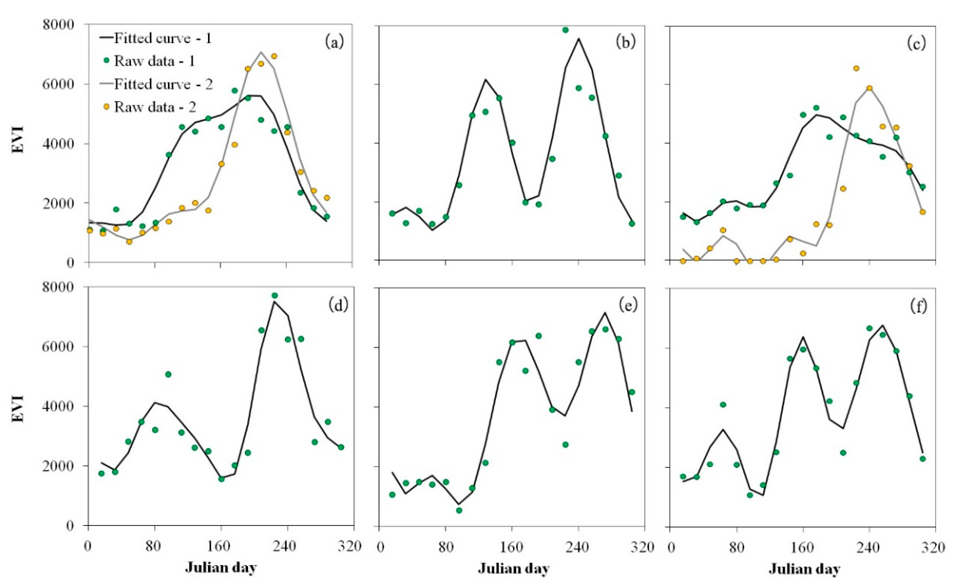
Figure 3 illustrates the existing cropping patterns in regions where double cropping is possible (Figure 3a,b) and those in regions where triple cropping is possible (Figure 3c–f). Curves with yellow dots (Figure 3a,c) indicate patterns in which double or triple cropping is possible, but only one cropping season was used. This circumstance existed, but was not in the majority. Therefore, for plots with a single cropping pattern, we did not differentiate patterns with different phases of the peak. For double cropping curves detected in regions where triple cropping is possible, there might be two circumstances: one is winter crops followed by summer crops (Figure 3d), and the other is double rice or early/late rice with other crops of a short growing season (Table 1) and without winter crops (Figure 3e). We differentiated these two patterns based on the phase of the first peak.
To detect the cropping seasons for each pixel, we firstly used a harmonic analysis of time series (HANTS) [47] to remove interference signals and restructure the time series curve of EVI. We excluded data after November to avoid fake peaks for winter wheat before it hibernates [47,48]. However, there still might be some fake peaks in the reconstructed EVI time series curve, such as the low peak of winter wheat before it hibernates. We additionally introduced some constraints before detecting the actual crop growing peaks. On the one hand, since the crop growth process usually lasts for a certain time, we defined a peak as an actual peak if it followed at least two continuous phases with a rising EVI value, and was followed by two continuous phases with decreasing EVI values. On the other hand, a plot in the triple cropping pattern could only occur in the area where the annual accumulated temperature above a base temperature was 5000 °C [49]. Based on the above terms, we could count the number of actual peaks in the reconstructed image pixel by pixel. For pixels with two peaks in the triple cropping region, we defined the pixel with the first peak occurring after June as the one in which double rice was planted (Figure 3e).
The entire procedure includes four steps:
(1) Defining the relationship between EVI values in adjacent phases is calculated as follows:
Δ a i = { 1       if   a i + 1 > a i 0       if   a i + 1 = a i 1       if   a i + 1 < a i  
where, a i and a i + 1 indicate the EVI values in phases i and i + 1 , and Δ a i denotes the relationship between a i and a i + 1 .
(2) The difference of adjacent Δ a i to determine the position of local peak and vale is calculated as follows:
Δ Δ a i = Δ a i + 1 Δ a i
If Δ Δ a i was less than zero, a local peak occurred in phase i 1 ; if Δ Δ a i was larger than zero, a local vale occurred in phase i 1 .
(3) Removing fake peaks according to the additional requirements mentioned above.
(4) Detecting the phase of the first peak for double cropping pixels in regions where triple cropping is possible.

3.2. Crop Harvest Area Allocation

We distributed the statistic harvest area of different crops onto different types of cropland defined by cropping patterns in each agricultural region. ArcGIS software was used in this process. We determined the harvest area of each crop in each grid by the following formulation:
H A i j = C A j × F c l j k × H I i j  
where H A i j is the harvest area of crop i in grid j in a 1 km × 1 km resolution; C A j is the area of cropland in grid j, which was obtained from the NLCD; F c l j k is the area fraction of cropland with pattern k to total cropland in grid j, which can be obtained from the MODIS-derived cropping pattern information described in Section 3.1; H I i j is the harvest index of crop i on cropland in pattern k, i.e., the harvest area of crop i per unit of cropland in pattern k; and H I i j is county-specific since the smallest granularity of harvest area is county. H I i j was calculated as follows:
H I i j = H A i l / C A k l
where H A i l is the harvest area of crop i in county l and C A k l is the area of cropland in pattern k in county l.
For each county, the cropland obtained from NLCD-C was divided into several cropping patterns based on the methods described in Section 3.1. Areas of cropland in pattern k were calculated by multiplying the proportion of cropland grids in pattern k by the total cropland area in this county. If the crop can be potentially distributed in two types of cropping patterns, such as groundnut in the North China Plain, we equally distributed the harvest area of this crop onto the two types of cropland. This means that only if we can get the harvest area of different varieties of this kind of crop, otherwise, for crops that can be potentially distributed in two cropping patterns in double cropping regions, the results based on our model will be similar to the commonly used average allocation. This situation occurs in 11 crop-region combinations out of the total 68 crop-region combinations.
The cropping patterns in Table 1 and phenology types in Figure 2 were used to allocate harvested area for each crop. Meanwhile, because of the discrepancies between statistical data and data derived from remote sensing images [50], as well as the misclassification of cropping patterns due to noise in the remote sensing data [51,52]), the area of cropland in a certain pattern might be smaller than the sum of the crops that are supposed to be distributed in this type of pattern, i.e., i H I i k   > 1. We developed the following principles, based on the crop calendar, to adjust the results to make it more reasonable:
  • For winter crops, we allocated them onto the cropland with a spring peak, that is, croplands in patterns 2-2, 3-2, and 3-4. If the sum area of the winter crops was larger than croplands with a spring peak, we allocated the excess area of winter crops onto the croplands with one cropping cycle, i.e., the croplands in patterns 2-1 and 3-1. We did not allocate winter crops onto pattern 3-3 because there was no spring peak in this type of cropland, according to our detection.
  • For spring or summer crops existing on single or double cropped lands, we allocated them onto the corresponding type of croplands, according to Table 1. For those counties with i H I i k   > 1 (k denotes patterns 2-2, 3-1, and 3-2), we firstly moved crops that could exist on two kinds of cropland patterns out from the croplands in pattern k, with i H I i k   > 1, to the croplands of pattern k, with i H I i k   < 1, to make sure the HI of all the crops in each grid were less than or equal to 1.
  • For spring or summer crops existing on triple cropped lands, we allocated them onto croplands where triple peaks were detected, or double peaks were detected, after June. For those counties with i H I i k   > 1 (k denotes patterns 3-3 and 3-4), we moved the crops marked in green that were not exclusively located in cropland in patterns 3-3 and 3-4 out onto another pattern where they might be located, so as to make sure the HI of all the crops in each grid were less than or equal to 1.

3.3. Verification and Accuracy Check

The accuracy of the methodologies proposed here is largely determined by the consistency between crop harvest area estimated from an area of cropping patterns derived from remote sensing data and the statistic crop harvest area that was supposed to be located on the corresponding cropping pattern. We applied linear regression to fit the above two sets of data, used the coefficient of determination to check the fitness, and used the slope to examine the consistency of these two sets of data.
We chose three pairs of cropping seasons in zones, with a relatively small group of crop types that can be planted, to examine the fitness (according to Table 1): (1) winter crops in potentially double cropped areas (WCD), exclusively planted with winter wheat and rapeseed; (2) winter crops in potentially triple cropped areas (WCT), exclusively planted with winter wheat, rapeseed, barley, and potato, and soybean in southern China (which can be distributed in both winter and the main season, but with very small area); and (3) main season crops in triple cropped areas (MCT), mainly including early rice, late rice, and some minority crops such as maize, soybean, and groundnut.
Analyses of the accuracy were applied on three levels: first, the overall fitness was obtained for all counties; second, counties of four provinces with the largest harvest area, together accounting for more than 70% of harvest area, were selected to examine the fitness separately; and third, we compared the fitness of each related province with its proportion of the harvest area of the crop of concern against the total area in China in order to test the assumption that the larger the planted area, the higher the accuracy would be.
We also employed paddy field areas from NLCD-C to check the accuracy of rice distribution. Although the paddy fields were not necessarily planting rice, most paddy fields are planted with rice, in China. We again used linear regression to fit these two datasets, the coefficient of determination to check the fitness, and the slope to examine the accuracy.
In order to compare the differences of the results from the different methods, we also employed the Shannon diversity index (SHDI). The SHDI is a measure of the disorder or uncertainty, which indicates the heterogeneity of a landscape or species. Here, we investigated the heterogeneity of patches in terms of harvest area for certain crops at the county level by SHDI. To do this, we compared the SHDI of our results with that of the average allocation model to examine which can offer more spatial details of crop distribution. The SHDI was calculated as follows:
S H D I j = i = 1 n P i j l n P i j
where P i j indicates the proportion of range i of harvest area of crop j at the grid level in the total harvest area of crop j in a county.

4. Results

4.1. Accuracy Assessment

4.1.1. Comparison of Area of Crop Groups Obtained by Remote Sensing with Statistical Data

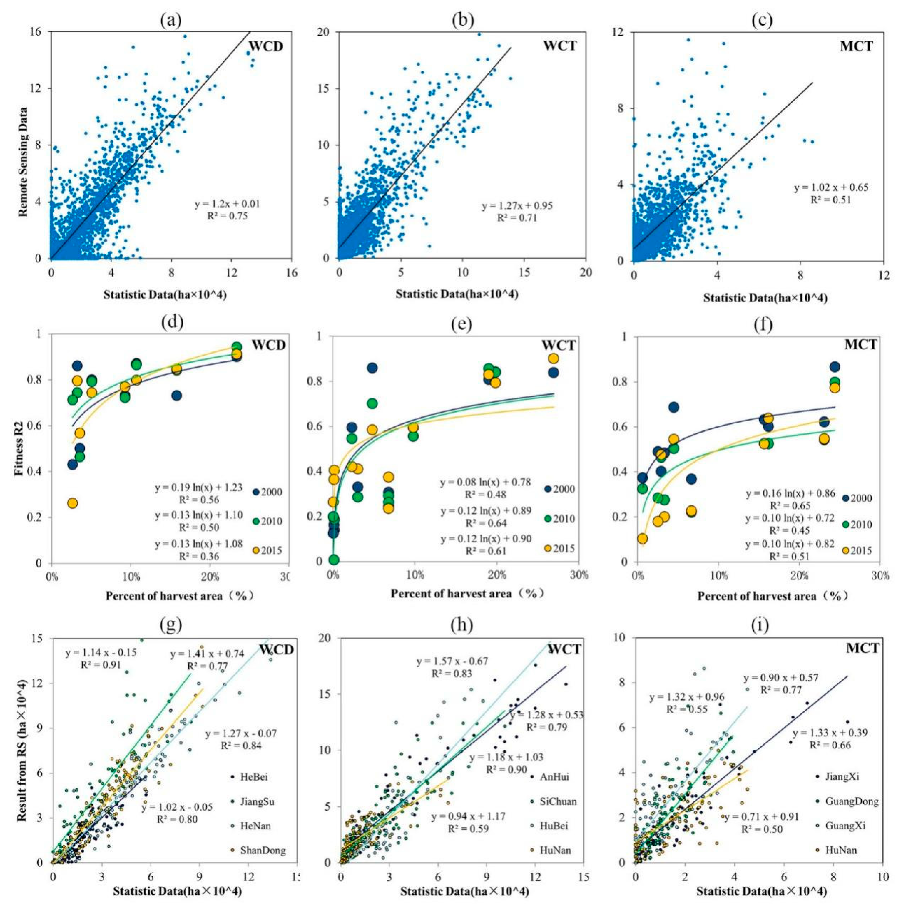
It is almost impossible to find true spatial distribution for all crops at the country level to verify our results. The accuracy of the area of cropland planted with different group of crops obtained from MODIS images is critical for the accuracy of the final results. The process of getting this value didn’t include statistical data, but it will be used to allocate the statistical crop area. Therefore, we checked the consistency between the area of crop groups in certain cropping seasons gained from remote sensing images and the one recoded by statistical data, based on which the reliability of our method could be assessed. The coefficient of determination for the results from the remote sensing images and statistical data across the country is 0.75 for WCD, 0.71 for WCT, and 0.51 for MCT, while the slope of the fitting model is 1.20 for WCD, 1.27 for WCT, and 1.02 for MCT (Figure 4a). Generally, the results obtained from remote sensing images matched the statistical data well.
The fitness of the two winter crops (WCD and WCT) was much better than that of the main season crops in triple cropped regions (MCT). For one thing, MCTs were concentrated in southern China, where landscape was fragile and mixed pixels were commonly found. For another thing, the planting season of MCTs was in the rainy season, which created the noise fluctuation of the EVI time series curve beyond the one reflecting growth process, leading to a relatively lower accuracy on crop seasons extraction in this region. The fitness of WCDs was higher than that of WCTs. Though they are both winter crops, WCDs were mainly concentrated in the North China Plain, where patches of cropland were large and mixed pixels were rare; however, WCTs were mostly located in southern China, where hills and mountains led to fragile landscapes and mixed pixels.
We further checked four provinces with the largest area for each pair in 2015, which together accounted for more than three quarters of the total harvest area of the corresponding crops. Most of these provinces had higher fitness in terms of R2 than the national average (Figure 4g–i), except the province with fourth largest harvest area for WCTs, which accounted for less than 10% of total harvest area. Generally, the ranges of R2 for WCTs (0.59–0.90) and MCTs (0.50–0.76) are larger than for WCDs (0.77–0.86). This can be attributed to the fact that the crop types included in WCDs were merely winter wheat and rapeseed exclusively planted in winter season, while more than three crops were included in WCTs and MCTs and some crops might be planted in other seasons, though with small areas, which will introduce higher uncertainty.
Analysis of the relationship between the fitness in terms of R2 and the proportion of the crop area for the corresponding province in national totals reveals that the model does better in provinces with larger areas of the crops of concern for all the three periods (Figure 4d–f). The R2 for WCDs are high in most provinces and less significant in the correlation with the proportion of crop area. However, the R2 for WCTs and MCTs has larger variation and is more significantly correlated with the proportion of crop area, which is mainly due to large variations in landscape [47], complexity of crop types, and noise in signals in the different provinces.

4.1.2. Comparison of Rice Distribution with Paddy Fields from the NLCD-C

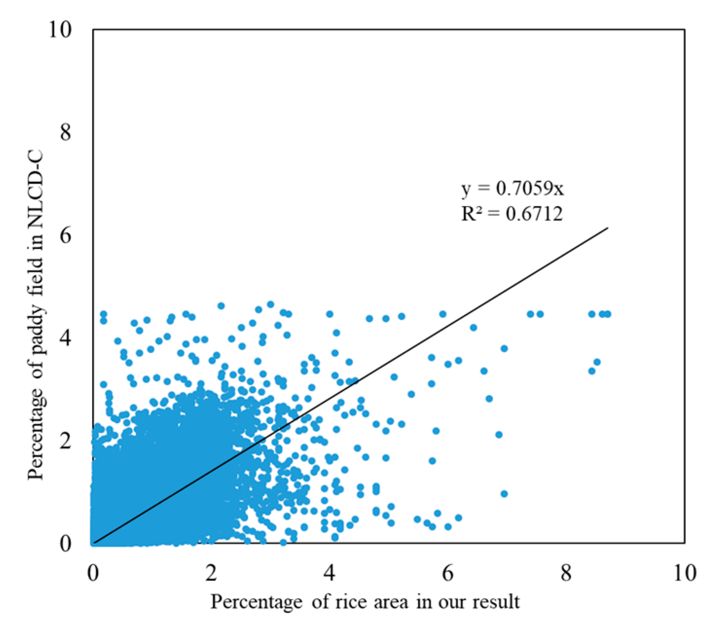
We also carried out quantitative validation when third-party independent crop maps were available. The NLCD-C is a national land use/cover database of China which was obtained by artificial visual interpretation based on remote sensing data with a spatial resolution of approximately 30 m. Rice, one of the most important crops, occupies the largest area of arable land in China. By assuming paddy fields were mostly used for growing rice, we calculate the area of paddy fields at a 1 × 1 km grid level for the NLCD-C. We further calculated the coefficient of determination (R2) and the slope of the fitting between the percent of rice (paddy field) area in each grid for the NLCD-C and our results. The value of R2 is 0.67 and the slope of the fitting is 0.71 (Figure 5), indicating a relatively high reliability. Compared with the validation results of other crop allocation models like SPAM (R2 for rice validation with the NLCD-C is 0.49), the accuracy of our crop allocation results is relatively high. There are potentially many factors affecting the discrepancy if we treat the NLCD-C as the truth, such as the accuracy of the NLCD-C and the difference in spatial resolution between the two datasets.

4.1.3. Comparison with Average Allocation Results

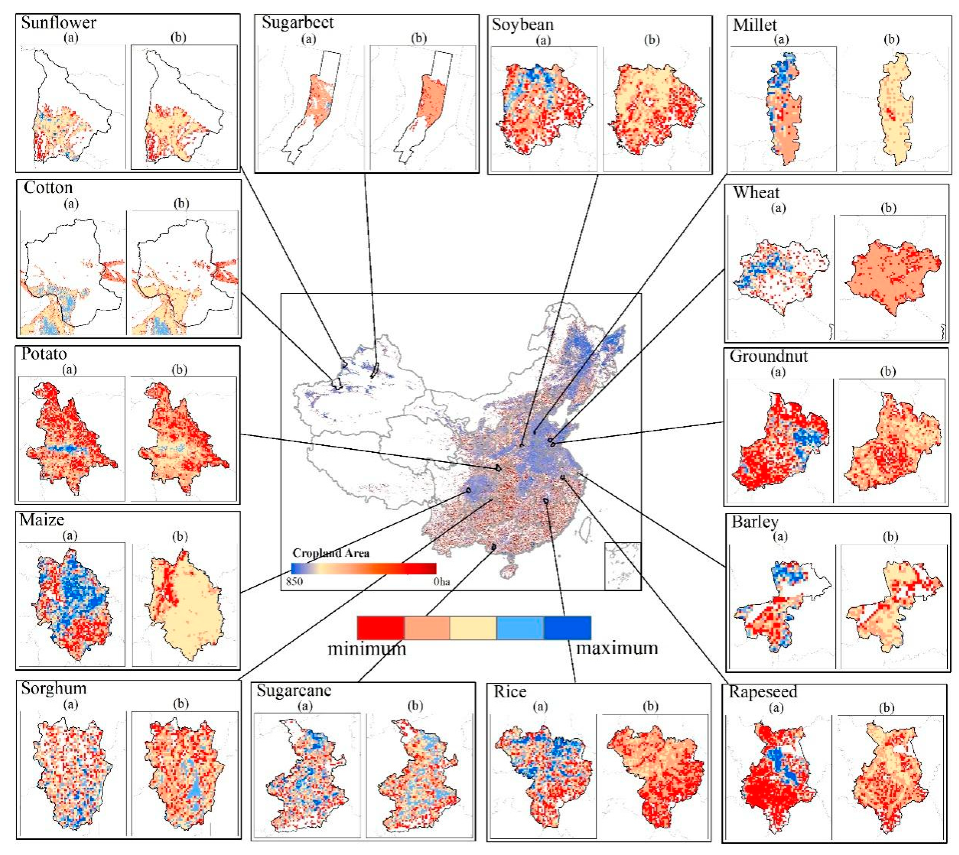
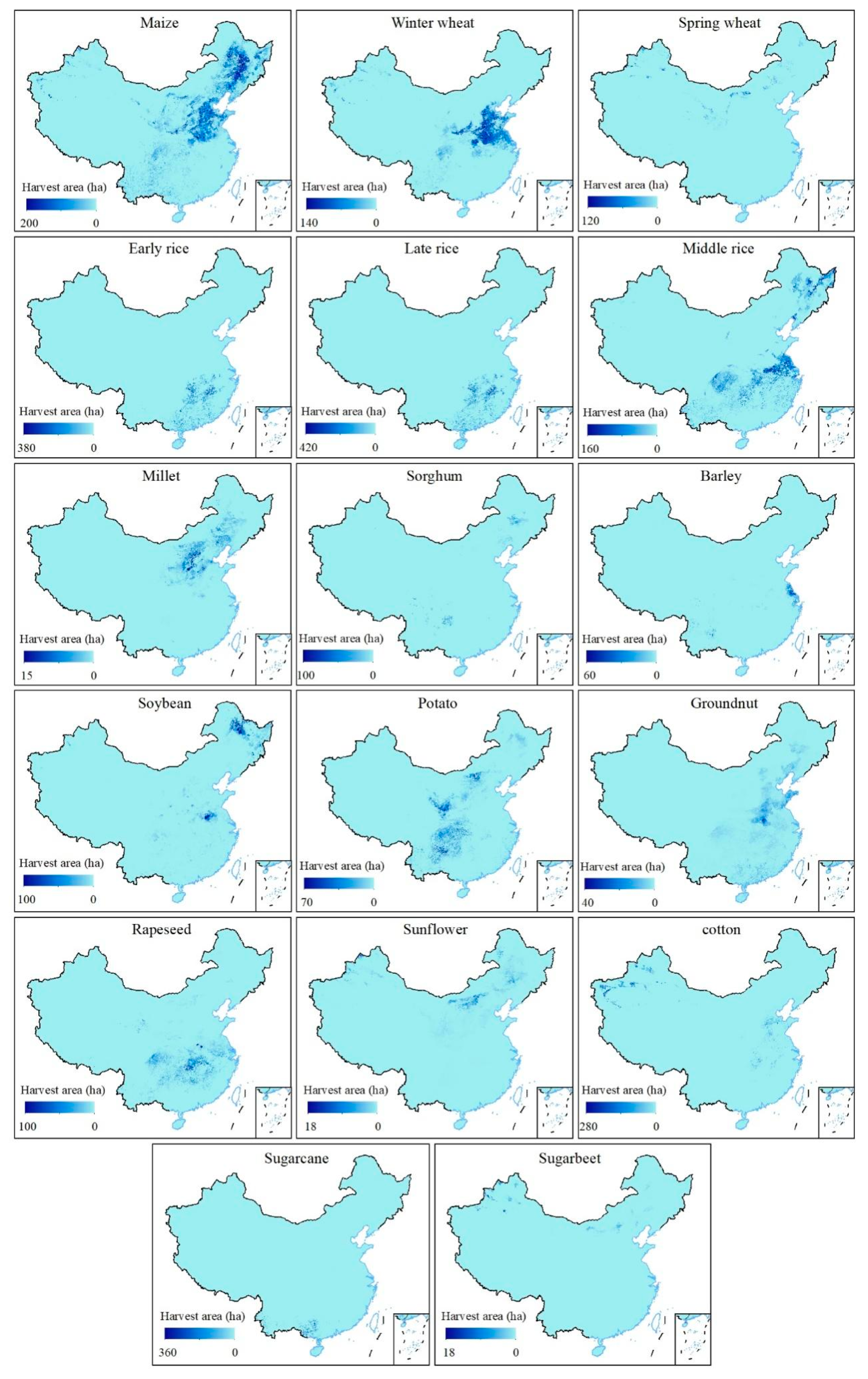
We compared the spatial details of our results with those obtained from the average allocation model both visually and quantitively. Figure 6 shows the distribution from the two models for the 14 crops (early rice, late rice, and middle rice were grouped as rice, and spring wheat and winter wheat were grouped as wheat) in counties with large harvest areas. Obviously, all 14 crops have larger variations in harvest area at the pixel level, and some crops, such as wheat, sugar beet, and barley, were concentratedly distributed in certain areas for our results, which cannot be detected by the average allocation model.
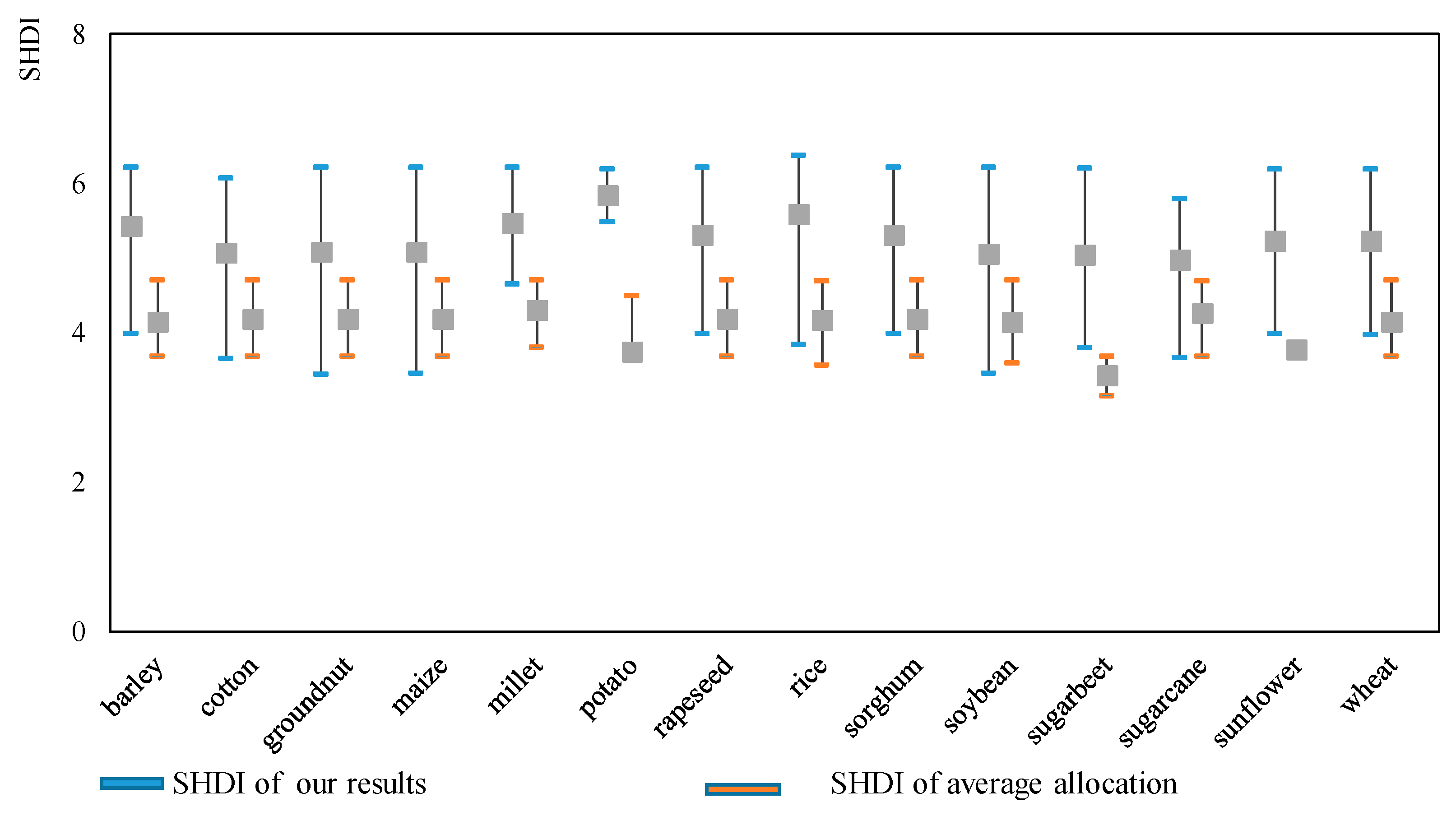
We further randomly chose eight counties to calculate the SHDI for spatial details within each county for each crop, respectively. A much larger SHDI was found in our results, with a maximum value between 6 and 7, while the maximum SHDI for the results based on the average allocation model was less than 5, meaning a higher spatial heterogeneity was detected by our model (Figure 7). The mean value of the SHDI of our results was about 1.3 times those from the average allocation model. Taking wheat in Xintai County of Shandong Province as an example, the SHDI for the average allocation was 4.69, whereas that of our allocation result was 5.97. Therefore, our results offer high spatial heterogeneity by effectively linking cropping seasons with crop types.

4.2. Patterns of Crop Distribution

Different crops are always distributed in different regions due to crop-specific climate suitability. Maize, mainly distributed in the North China Plain and northeastern China (Figure 8), has the largest harvest area, and approximately 32% of cropland was planted with maize for one crop season in 2015. Wheat was concentrated in the North China Plain, northeastern China, and northwestern China, within which less than 10% was spring wheat, which was mainly distributed in northern China, where single cropping was applied. Double cropped rice, including early rice and late rice, was mainly planted south of the Yangtze River, whereas middle rice can also be found in northeastern China. Respectively, 5%, 6%, and 11% of the croplands were planted with early rice, late rice, and middle rice for one crop season in 2015. About 1% of the croplands were planted with the other three types of cereals in one crop season, i.e., millet (the North China Plain), sorghum (southwestern China and northeastern China), and barley (southwestern China and eastern China) (Figure 8).
Besides the three major staple crops, rapeseed and soybean were the two crops with the largest areas, and about 5% of cropland was planted with these two crops in 2015. Rapeseed was mainly concentrated in southern China, while soybean was mostly planted in northeastern China and south of the North China Plain (Figure 8). Potato, planted on 3% of the cropland, was mainly concentrated in the second ladder of topography, where the temperature is moderate. Sunflower and sugar beet were the two crops other than spring wheat that were mainly planted in northern China, while sugarcane was the only one distributed in southern China, especially in Guangxi province.

4.3. Change Patterns of Major Crops

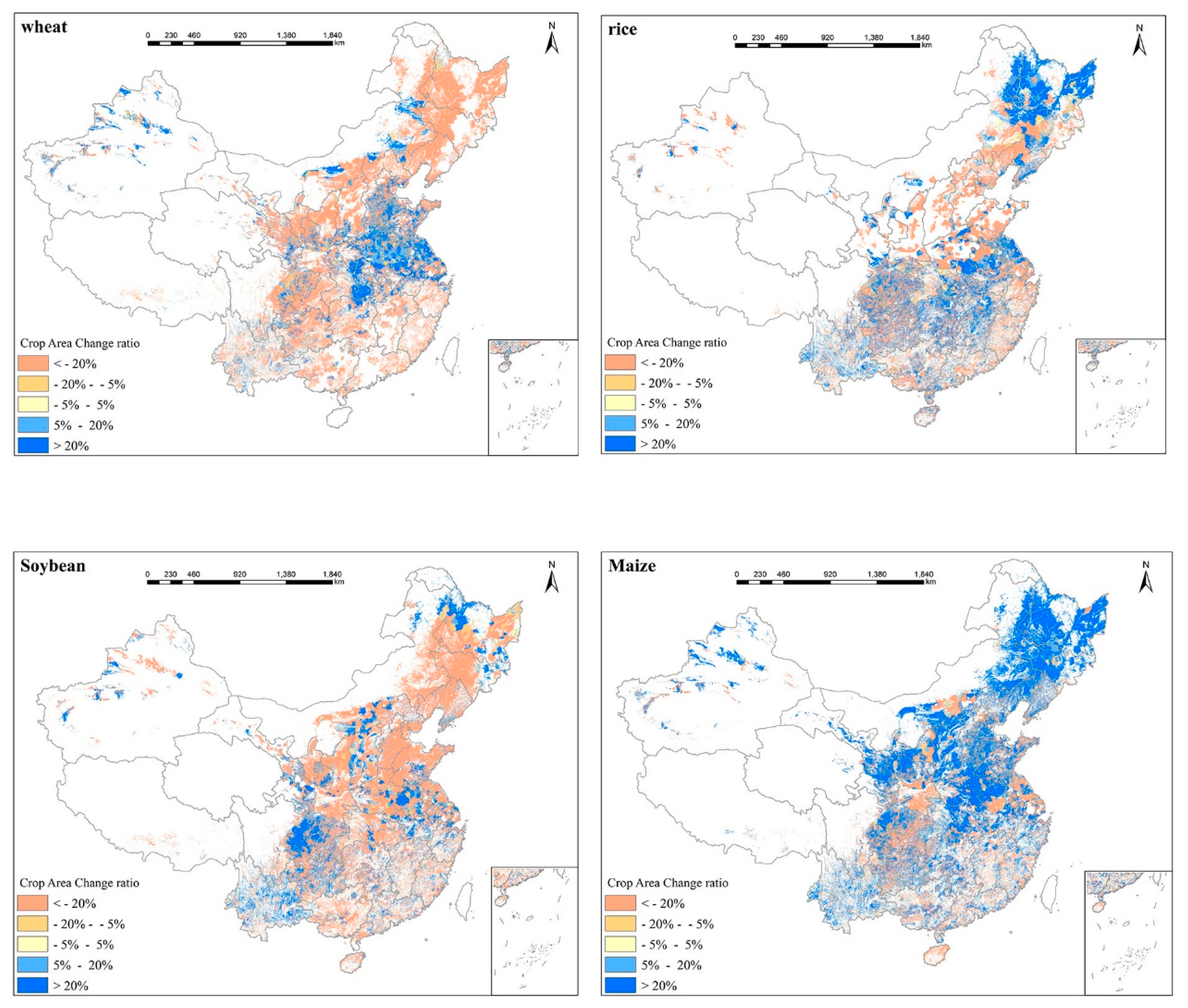
From 2000 to 2015, among the 14 major crops, the planting area of maize increased significantly, and the planting area of potato, sugarcane, peanuts, and rape increased slightly. For other crops, the planting area decreased. Here, we focus on the four major crops, i.e., wheat, rice, maize, and soybean, to dig into the change patterns of their distribution (Figure 9). We separated the grid cells into two types: cells with increased area and cells with decreased area, and we defined the grid cells with area change rates larger than 20% as high change intensity.
For wheat, the cells with decreased area accounted for 74.92% of all cells with area changed. High decrease intensity cells were mainly located in Heilongjiang Province, the Inner Mongolia Autonomous Region, Sichuan Province, and Shaanxi Province, with more than 30% of the cells showing a largely decreased area in these provinces. The high increase intensity cells were mainly located in the Inner Mongolia Autonomous Region, Henan Province, Hubei Province, and Shandong Province, with nearly 40% of the cells showing a largely increased area in these provinces. The Inner Mongolia Autonomous Region had regions with areas of wheat that shifted a lot, as it had plenty of cells with both high decrease intensity and high increase intensity concentratedly distributed.
For rice, the cells with decreased area accounted for 57.32% of all cells with area changed. High decrease intensity cells were mainly located in Sichuan Province, Guizhou Province, the Inner Mongolia Autonomous Region, and Guangxi Province, with more than 20% of the cells showing a largely decreased area in these provinces. The high increase intensity cells were mainly located in Heilongjiang Province, Hunan Province, Yunnan Province, and Sichuan Province, with nearly 40% of the cells showing a largely increased area in these provinces. Sichuan Province had regions with areas of rice that shifted a lot, as it had plenty of cells with both high decrease intensity and high increase intensity concentratedly distributed.
For soybean, the cells with decreased area accounted for 59.00% of all cells with area changed. High decrease intensity cells were mainly located in the Inner Mongolia Autonomous Region, Heilongjiang Province, Shaanxi Province, and Hebei Province, with more than 25% of the cells showing a largely decreased area in these provinces. The high increase intensity cells were mainly located in Sichuan Province, Yunnan Province, Heilongjiang Province, and Anhui Province, with nearly 40% of the cells showing a largely increased area in these provinces. Heilongjiang Province had regions with areas of soybean that shifted a lot, as it had plenty of cells with both high decrease intensity and high increase intensity concentratedly distributed.
For maize, the cells with increased area accounted for 62.29% of all cells with area changed. High decrease intensity cells were mainly located in Shaanxi Province, Sichuan Province, Guizhou Province, and Guangxi Province, with more than 25% of the cells showing a largely decreased area in these provinces. The high increase intensity cells were mainly located in Heilongjiang Province, the Inner Mongolia Autonomous Region, Henan Province, and Jilin Province, with nearly 40% of the cells showing a largely increased area in these provinces.

5. Discussion

Remote sensing techniques have been considered an efficient method for crop distribution mapping. Previous methods mainly focused on the detection of only some major crops [53,54]. When referring to all kinds of crop mapping, fused remote sensing data and statistical data were commonly used; however, the average allocation method [14] or predicting models [36,37,38], such as the cross-entropy approach, were the most popular ones. We mapped 14 crops by combining crop season information derived from remote sensing images and crop harvest area from statistical data. We compared the crop areas estimated from the remote sensing images with national statistical data at the county level. The results showed a high consistency between these two values, meaning that the methodologies proposed here are effective. The error mainly comes from mixed pixels.
Inaccuracy of the results mainly comes from large numbers of mixed pixels in the fragile landscape of areas with complex crop planting patterns. From our results, we could see that the slopes of the fitting model for all three pairs of cropping seasons in zones were larger than 1 (Figure 4), indicating that the results derived from the remote sensing data were mostly larger than those from the statistical data. This is mainly because pixels in the remote sensing images though are recognized as pure cropland that always includes paths, channels, ponds, etc. in fields [47]. Areas of this infrastructure were accounted for in the remote sensing results; however, they were excluded in the statistical data. The more fragile the landscape of cropland is, the higher the inaccuracy that would occur [52,55].
Some studies have explored methods for reducing the impact of mixed pixels on the accuracy of crop mapping [56,57]. One effective way is to integrate images with high spatial resolution with those having lower spatial resolution, such as fusing Landsat data and MODIS data, to improve the spatial resolution of the datasets; however, the large amount of data was generally a challenge when referring to large-scale research [58]. Some studies have employed decision trees to try to use a small amount of data to map cropping information efficiently [59]. Fortunately, the emergence of Google Earth Engine enabled studies based on images with moderate resolution [50]. Another solution is to map fractional crop distribution by building up estimation models that illustrate the relationship between the vegetation index from data with low spatial resolution and the information at a higher resolution. In the future, methods similar to the above, and other effective methods that can improve accuracy, can be used in crop allocation to reduce the impact of mixed pixels on accuracy.
Using low–medium resolution data, such as MODIS data, or using moderate resolution data, such as Landsat and Sentinel, for crop types that were successfully identified by remote sensing data at the regional or national scale are mainly concentrated on some major crops with large planting areas, for example, rice [25,26,27], wheat [28], maize [29], soybean [30], and sugarcane [31], and mostly different combinations of these crops [32,33,34,35]. Crops with low popularity are generally not included due to their lower visibility on the signals from remote sensing images. Based on the crop seasons obtained from remote sensing, statistical data, and the crop phenology information, this paper draws the spatial distribution map of 14 crops. These crops include not only the main food crops, but also some smaller kinds of crops, such as sugarcane, peanut, barley, sunflower, and so on. The spatial distribution maps of these crops can show more detailed spatial distribution information of crops in a larger space.
We also compared our results of area change with those of other researchers. The planting area of rice increased obviously in Heilongjiang Province, which was consistent with Lu’s research results, which found that the total cultivated area of rice in Heilongjiang Province increased largely from 1993 to 2011 and it expanded spatially to the northern and eastern parts of the Sanjiang Plain. Other findings consistent with this study found that the rice planting area in Northeastern China expanded quickly and increased by nearly 4.5 times during the period from 1980–2010.
Some studies also paid attention to cropping patterns in single crop regions. For example, the peak time of time series curves of VIs for spring maize and spring wheat in northern China is usually different from those of soybean and summer maize, which could be used to further differentiate these crops [59]. In the future, we could collect more detailed data on the harvest areas of different crops to utilize this information. Some other studies found that cotton planted in the North China Plain always has a longer cropping season when compared with single cropped maize [60]. This reminds us that the length of cropping season can be used to further distinguish cropping patterns in order to get more detailed crop distribution information. In conclusion, more information about the peak of VIs time series curves and the length of cropping season perhaps can be used to improve the accuracy of crop mapping.

6. Conclusions

Crop distribution has been recognized as an essential basis for evaluating food security, environmental change, and global climate change. Tradeoffs between spatial resolution and the number of crops of concern always exist in crop mapping. In this study, we present an improved crop allocation model by combining cropping season data detected from remote sensing images and the regional crop calendar, aiming to provide more spatially resolved crop maps with a larger span. Verification of the model showed that the harvest areas of crops/crop groups obtained by cropping seasons derived from remote sensing images matched well with the statistical data, indicating that our model is a reliable one for national crop mapping. The fitness between these two datasets on the provincial level was largely affected by landscape characteristics in that the flat areas always had a higher fitness, and thus a high accuracy due to fewer mixed pixels. Moreover, the larger a provincial harvest area is, the higher its fitness. Basically, our proposed model can map crops in a greater detail compared to the commonly used average allocation model, and it is suitable for large-scale crop mapping.

Author Contributions

Conceptualization, L.Z. and Y.W.; methodology, L.Z. and Y.W.; software, Z.Z. and X.Z.; validation, X.Z. and X.W.; formal analysis, Y.W. and L.Z.; investigation, Y.W., F.S., and X.W.; resources, Z.Z.; data curation, Z.Z.; writing—original draft preparation, Y.W.; writing—review and editing, L.Z.; visualization, X.Z. and X.W.; supervision, Z.Z. and L.Z.; project administration, L.Z.; funding acquisition, L.Z. All authors have read and agreed to the published version of the manuscript.

Funding

This research was funded by the National Key R&D Program of China (2017YFE0104600).

Data Availability Statement

The data presented in this study are available on request from the corresponding author. The data are not publicly available due to privacy.

Conflicts of Interest

The authors declare no conflict of interest.

References

  1. Foley, J.A.; DeFries, R.; Asner, G.P.; Barford, C.; Bonan, G.; Carpenter, S.R.; Chapin, F.S.; Coe, M.T.; Daily, G.C.; Gibbs, H.K.; et al. Global Consequences of Land Use. Science 2005, 309, 570–574. [Google Scholar] [CrossRef] [PubMed] [Green Version]
  2. Kastner, T.; Rivas, M.J.I.; Koch, W.; Nonhebel, S. Global changes in diets and the consequences for land requirements for food. Proc. Natl. Acad. Sci. USA 2012, 109, 6868–6872. [Google Scholar] [CrossRef] [PubMed] [Green Version]
  3. West, P.C.; Gerber, J.S.; Engstrom, P.M.; Mueller, N.D.; Brauman, K.A.; Carlson, K.M.; Cassidy, E.S.; Johnston, M.; MacDonald, G.K.; Ray, D.K.; et al. Leverage points for improving global food security and the environment. Science 2014, 345, 325–328. [Google Scholar] [CrossRef] [PubMed] [Green Version]
  4. Zuo, L.; Zhang, Z.; Carlson, K.M.; MacDonald, G.K.; Brauman, K.A.; Liu, Y.; Zhang, W.; Zhang, H.; Wu, W.; Zhao, X.; et al. Progress towards sustainable intensification in China challenged by land-use change. Nat. Sustain. 2018, 1, 304–313. [Google Scholar] [CrossRef]
  5. Zhang, X.; Davidson, E.A.; Mauzerall, D.L.; Searchinger, T.D.; Dumas, P.; Shen, Y. Managing nitrogen for sustainable development. Nature 2015, 528, 51–59. [Google Scholar] [CrossRef] [Green Version]
  6. Wang, S.; Azzari, G.; Lobell, D.B. Crop type mapping without field-level labels: Random forest transfer and unsupervised clustering techniques. Remote Sens. Environ. 2019, 222, 303–317. [Google Scholar] [CrossRef]
  7. United Nations, Department of Economic and Social Affairs, Population Division. World Population Prospects 2019. Online Edition. Rev. 1. 2019. Available online: https://population.un.org/wpp/ (accessed on 15 February 2022).
  8. FAOSTAT. FAOSTAT Online Statistical Service. Available online: http://www.fao.org/faostat/en/#data (accessed on 9 July 2020).
  9. Zhao, C.; Liu, B.; Piao, S.; Wang, X.; Lobell, D.B.; Huang, Y.; Huang, M.; Yao, Y.; Bassu, S.; Ciais, P.; et al. Temperature increase reduces global yields of major crops in four independent estimates. Proc. Natl. Acad. Sci. USA 2017, 114, 9326–9331. [Google Scholar] [CrossRef] [Green Version]
  10. Waldner, F.; De Abelleyra, D.; Verón, S.R.; Zhang, M.; Wu, B.; Plotnikov, D.; Bartalev, S.; Lavreniuk, M.; Skakun, S.; Kussul, N.; et al. Towards a set of agrosystem-specific cropland mapping methods to address the global cropland diversity. Int. J. Remote Sens. 2016, 37, 3196–3231. [Google Scholar] [CrossRef] [Green Version]
  11. FAO. Food and Agriculture Organization of the United Nations. Available online: http://www.fao.org/ (accessed on 15 February 2022).
  12. NBS. China National Statistical Yearbook. Available online: http://www.stats.gov.cn/english/ (accessed on 9 July 2020).
  13. Liu, Z.; Yang, P.; Wu, W.; Li, Z.; You, L. Spatio-temporal changes in Chinese crop patterns over the past three decades. Acta Geogr. Sin. 2016, 71, 840–851. [Google Scholar]
  14. Monfreda, C.; Ramankutty, N.; Foley, J.A. Farming the planet: 2. Geographic distribution of crop areas, yields, physiological types, and net primary production in the year 2000. Glob. Biogeochem. Cycles 2008, 2, 1–19. [Google Scholar] [CrossRef]
  15. Guo, Y.; Xia, H.; Pan, L.; Zhao, X.; Li, R. Mapping the Northern Limit of Double Cropping Using a Phenology-Based Algorithm and Google Earth Engine. Remote Sens. 2022, 14, 1004. [Google Scholar] [CrossRef]
  16. Wardlow, B.D.; Egbert, S.L.; Kastens, J.H. Analysis of time-series MODIS 250 m vegetation index data for crop classification in the U.S. Central Great Plains. Remote Sens. Environ. 2007, 108, 290–310. [Google Scholar] [CrossRef] [Green Version]
  17. Zhu, L.; Radeloff, V.C.; Ives, A.R. Improving the mapping of crop types in the Midwestern U.S. by fusing Landsat and MODIS satellite data. Int. J. Appl. Earth Obs. Geoinf. 2017, 58, 1–11. [Google Scholar] [CrossRef]
  18. Wang, C.; Fan, Q.; Li, Q.; SooHoo, W.M.; Lu, L. Energy crop mapping with enhanced TM/MODIS time series in the BCAP agricultural lands. ISPRS J. Photogramm. Remote Sens. 2017, 124, 133–143. [Google Scholar] [CrossRef] [Green Version]
  19. Li, Q.; Wang, C.; Zhang, B.; Lu, L. Object-Based Crop Classification with Landsat-MODIS Enhanced Time-Series Data. Remote Sens. 2015, 7, 16091–16107. [Google Scholar] [CrossRef] [Green Version]
  20. Griffiths, P.; Nendel, C.; Hostert, P. Intra-annual reflectance composites from Sentinel-2 and Landsat for national-scale crop and land cover mapping. Remote Sens. Environ. 2019, 220, 135–151. [Google Scholar] [CrossRef]
  21. Dong, J.; Xiao, X.; Menarguez, M.A.; Zhang, G.; Qin, Y.; Thau, D.; Biradar, C.; Moore, B., III. Mapping paddy rice planting area in northeastern Asia with Landsat 8 images, phenology-based algorithm and Google Earth Engine. Remote Sens. Environ. 2016, 185, 142–154. [Google Scholar] [CrossRef] [Green Version]
  22. Kussul, N.; Lemoine, G.; Gallego, F.J.; Skakun, S.V.; Lavreniuk, M.; Shelestov, A.Y. Parcel-Based Crop Classification in Ukraine Using Landsat-8 Data and Sentinel-1A Data. IEEE J. Sel. Top. Appl. Earth Obs. Remote Sens. 2016, 9, 2500–2508. [Google Scholar] [CrossRef]
  23. Skakun, S.; Vermote, E.; Roger, J.-C.; Franch, B. Combined use of Landsat-8 and Sentinel-2A images for winter crop mapping and winter wheat yield assessment at regional scale. AIMS Geosci. 2017, 3, 163. [Google Scholar] [CrossRef]
  24. Kpienbaareh, D.; Sun, X.; Wang, J.; Luginaah, I.; Bezner Kerr, R.; Lupafya, E.; Dakishoni, L. Crop type and land cover mapping in northern Malawi using the integration of sentinel-1, sentinel-2, and planetscope satellite data. Remote Sens. 2021, 13, 700. [Google Scholar] [CrossRef]
  25. Xiao, X.; Boles, S.; Frolking, S.; Li, C.; Babu, J.Y.; Salas, W.; Moore, B. Mapping paddy rice agriculture in South and Southeast Asia using multi-temporal MODIS images. Remote Sens. Environ. 2006, 100, 95–113. [Google Scholar] [CrossRef]
  26. Gumma, M.K.; Thenkabail, P.S.; Maunahan, A.; Islam, S.; Nelson, A. Mapping seasonal rice cropland extent and area in the high cropping intensity environment of Bangladesh using MODIS 500 m data for the year 2010. ISPRS J. Photogramm. Remote Sens. 2014, 91, 98–113. [Google Scholar] [CrossRef]
  27. Onojeghuo, A.O.; Blackburn, G.A.; Wang, Q.; Atkinson, P.M.; Kindred, D.; Miao, Y. Rice crop phenology mapping at high spatial and temporal resolution using downscaled MODIS time-series. GIS Sci. 2018, 55, 659–677. [Google Scholar] [CrossRef] [Green Version]
  28. Pan, Y.; Li, L.; Zhang, J.; Liang, S.; Zhu, X.; Sulla-Menashe, D. Winter wheat area estimation from MODIS-EVI time series data using the Crop Proportion Phenology Index. Remote Sens. Environ. 2012, 119, 232–242. [Google Scholar] [CrossRef]
  29. Chen, Y.; Hou, J.; Huang, C.; Zhang, Y.; Li, X. Mapping Maize Area in Heterogeneous Agricultural Landscape with Multi-Temporal Sentinel-1 and Sentinel-2 Images Based on Random Forest. Remote Sens. 2021, 13, 2988. [Google Scholar] [CrossRef]
  30. Song, X.-P.; Potapov, P.V.; Krylov, A.; King, L.; Di Bella, C.M.; Hudson, A.; Khan, A.; Adusei, B.; Stehman, S.V.; Hansen, M.C. National-scale soybean mapping and area estimation in the United States using medium resolution satellite imagery and field survey. Remote Sens. Environ. 2017, 190, 383–395. [Google Scholar] [CrossRef]
  31. Wang, J.; Xiao, X.; Liu, L.; Wu, X.; Qin, Y.; Steiner, J.L.; Dong, J. Mapping sugarcane plantation dynamics in Guangxi, China, by time series Sentinel-1, Sentinel-2 and Landsat images. Remote Sens. Environ. 2020, 247, 111951. [Google Scholar] [CrossRef]
  32. Skakun, S.; Franch, B.; Vermote, E.; Roger, J.-C.; Becker-Reshef, I.; Justice, C.; Kussul, N. Early season large-area winter crop mapping using MODIS NDVI data, growing degree days information and a Gaussian mixture model. Remote Sens. Environ. 2017, 195, 244–258. [Google Scholar] [CrossRef]
  33. Arvor, D.; Jonathan, M.; Meirelles, M.S.P.; Dubreuil, V.; Durieux, L. Classification of MODIS EVI time series for crop mapping in the state of Mato Grosso, Brazil. Int. J. Remote Sens. 2011, 32, 7847–7871. [Google Scholar] [CrossRef]
  34. Zhong, L.; Hu, L.; Yu, L.; Gong, P.; Biging, G.S. Automated mapping of soybean and corn using phenology. ISPRS J. Photogramm. Remote Sens. 2016, 119, 151–164. [Google Scholar] [CrossRef] [Green Version]
  35. Ofori-Ampofo, S.; Pelletier, C.; Lang, S. Crop Type Mapping from Optical and Radar Time Series Using Attention-Based Deep Learning. Remote Sens. 2021, 13, 4668. [Google Scholar] [CrossRef]
  36. Jackson, N.D.; Konar, M.; Debaere, P.; Estes, L. Probabilistic global maps of crop-specific areas from 1961 to 2014. Environ. Res. Lett. 2019, 14, 094023. [Google Scholar] [CrossRef]
  37. You, L.; Wood, S.; Wood-Sichra, U.; Wu, W. Generating global crop distribution maps: From census to grid. Agric. Syst. 2014, 127, 53–60. [Google Scholar] [CrossRef] [Green Version]
  38. Tan, J.; Li, Z.; Yang, P.; Yu, Q.; Zhang, L.; Wu, W.; Tang, P.; Liu, Z.; You, L. Spatial evaluation of crop maps by the spatial production allocation model in China. J. Appl. Remote Sens. 2014, 8, 085197. [Google Scholar] [CrossRef]
  39. Khan, M.R.; De Bie, C.A.; Van Keulen, H.; Smaling, E.M.A.; Real, R. Disaggregating and mapping crop statistics using hypertemporal remote sensing. Int. J. Appl. Earth Obs. 2010, 12, 36–46. [Google Scholar] [CrossRef]
  40. Zhang, Z.; Wang, X.; Zhao, X.; Liu, B.; Yi, L.; Zuo, L.; Wen, Q.; Liu, F.; Xu, J.; Hu, S. A 2010 update of National Land Use/Cover Database of China at 1:100,000 scale using medium spatial resolution satellite images. Remote Sens. Environ. 2014, 149, 142–154. [Google Scholar] [CrossRef]
  41. Hu, Q.; Yin, H.; Friedl, M.A.; You, L.; Li, Z.; Tang, H.; Wu, W. Integrating coarse-resolution images and agricultural statistics to generate sub-pixel crop type maps and reconciled area estimates. Remote Sens. Environ. 2021, 258, 112365. [Google Scholar] [CrossRef]
  42. CAAS. AgriData, (Chinese Academy of Agricultural Sciences, CAAS, 2014). Available online: http://www.agridata.cn/default.aspx (accessed on 7 March 2018).
  43. NBSC. National Data: Online Statistical Service, (National Bureau of Statistics of the People’s Republic of China 2017). Available online: http://data.stats.gov.cn/index.htm (accessed on 12 July 2018).
  44. Tóth, G.; Kozlowski, B.; Prieler, S.; Wiberg, D. Global Agro-ecological Zones. Available online: https://www.gaez.iiasa.ac.at/docs/GAEZ_User_Guide.pdf (accessed on 15 November 2019).
  45. Muhammad, S.; Zhan, Y.; Wang, L.; Hao, P.; Niu, Z. Major crops classification using time series MODIS EVI with adjacent years of ground reference data in the US state of Kansas. Optik 2016, 127, 1071–1077. [Google Scholar] [CrossRef]
  46. Zhang, J.; Feng, L.; Yao, F. Improved maize cultivated area estimation over a large scale combining MODIS-EVI time series data and crop phenological information. Isprs J. Photogramm. Remote Sens. 2014, 94, 102–113. [Google Scholar] [CrossRef]
  47. Zuo, L.-J.; Wang, X.; Liu, F.; Yi, L. Spatial Exploration of Multiple Cropping Efficiency in China Based on Time Series Remote Sensing Data and Econometric Model. J. Integr. Agric. 2013, 12, 903–913. [Google Scholar] [CrossRef]
  48. Guo, Y.; Xia, H.; Pan, L.; Zhao, X.; Li, R.; Bian, X.; Wang, R.; Yu, C. Development of a New Phenology Algorithm for Fine Mapping of Cropping Intensity in Complex Planting Areas Using Sentinel-2 and Google Earth Engine. ISPRS Int. J. Geo-Inf. 2021, 10, 587. [Google Scholar] [CrossRef]
  49. Liu, X. Farming System; China Agriculture Press: Beijing, China, 1982. (In Chinese) [Google Scholar]
  50. Liu, L.; Xiao, X.M.; Qin, Y.W.; Wang, J.; Xu, X.L.; Hu, Y.M.; Qiao, Z. Mapping cropping intensity in China using time series Landsat and Sentinel-2 images and Google Earth Engine. Remote Sens. Environ. 2020, 239, 13. [Google Scholar] [CrossRef]
  51. Chen, Y.L.; Lu, D.S.; Moran, E.; Batistella, M.; Dutra, L.V.; Sanches, I.D.; da Silva, R.F.B.; Huang, J.F.; Luiz, A.J.B.; de Oliveira, M.A.F. Mapping croplands, cropping patterns, and crop types using MODIS time-series data. Int. J. Appl. Earth Obs. Geoinf. 2018, 69, 133–147. [Google Scholar] [CrossRef]
  52. Feyisa, G.L.; Palao, L.K.; Nelson, A.; Gumma, M.K.; Paliwal, A.; Win, K.T.; Nge, K.H.; Johnson, D.E. Characterizing and mapping cropping patterns in a complex agro-ecosystem: An iterative participatory mapping procedure using machine learning algorithms and MODIS vegetation indices. Comput. Electron. Agric. 2020, 175, 105595. [Google Scholar] [CrossRef]
  53. Teluguntla, P.; Thenkabail, P.S.; Xiong, J.; Gumma, M.K.; Congalton, R.G.; Oliphant, A.; Poehnelt, J.; Yadav, K.; Rao, M.; Massey, R. Spectral matching techniques (SMTs) and automated cropland classification algorithms (ACCAs) for mapping croplands of Australia using MODIS 250-m time-series (2000–2015) data. Int. J. Digit. Earth 2017, 10, 944–977. [Google Scholar] [CrossRef] [Green Version]
  54. Brown, J.C.; Kastens, J.H.; Coutinho, A.C.; Victoria, D.D.; Bishop, C.R. Classifying multiyear agricultural land use data from Mato Grosso using time-series MODIS vegetation index data. Remote Sens. Environ. 2013, 130, 39–50. [Google Scholar] [CrossRef] [Green Version]
  55. Chen, Y.; Song, X.; Wang, S.; Huang, J.; Mansaray, L.R. Impacts of spatial heterogeneity on crop area mapping in Canada using MODIS data. ISPRS J. Photogramm. Remote Sens. 2016, 119, 451–461. [Google Scholar] [CrossRef]
  56. Ozdogan, M. The spatial distribution of crop types from MODIS data: Temporal unmixing using Independent Component Analysis. Remote Sens. Environ. 2010, 114, 1190–1204. [Google Scholar] [CrossRef]
  57. Dong, T.F.; Liu, J.G.; Qian, B.D.; Zhao, T.; Jing, Q.; Geng, X.Y.; Wang, J.F.; Huffman, T.; Shang, J.L. Estimating winter wheat biomass by assimilating leaf area index derived from fusion of Landsat-8 and MODIS data. Int. J. Appl. Earth Obs. Geoinf. 2016, 49, 63–74. [Google Scholar] [CrossRef]
  58. Gao, F.; Anderson, M.C.; Zhang, X.; Yang, Z.; Alfieri, J.G.; Kustas, W.P.; Mueller, R.; Johnson, D.M.; Prueger, J.H. Toward mapping crop progress at field scales through fusion of Landsat and MODIS imagery. Remote Sens. Environ. 2017, 188, 9–25. [Google Scholar] [CrossRef] [Green Version]
  59. Zuo, L.; Dong, T.; Wang, X.; Zhao, X.; Yi, L. Multiple cropping index of Northern China based on MODIS/EVI. Trans. Chin. Soc. Agric. Eng. 2009, 25, 141–146. [Google Scholar]
  60. Hao, P.Y.; Tang, H.J.; Chen, Z.X.; Meng, Q.Y.; Kang, Y.P. Early-season crop type mapping using 30-m reference time series. J. Integr. Agric. 2020, 19, 1897–1911. [Google Scholar] [CrossRef]
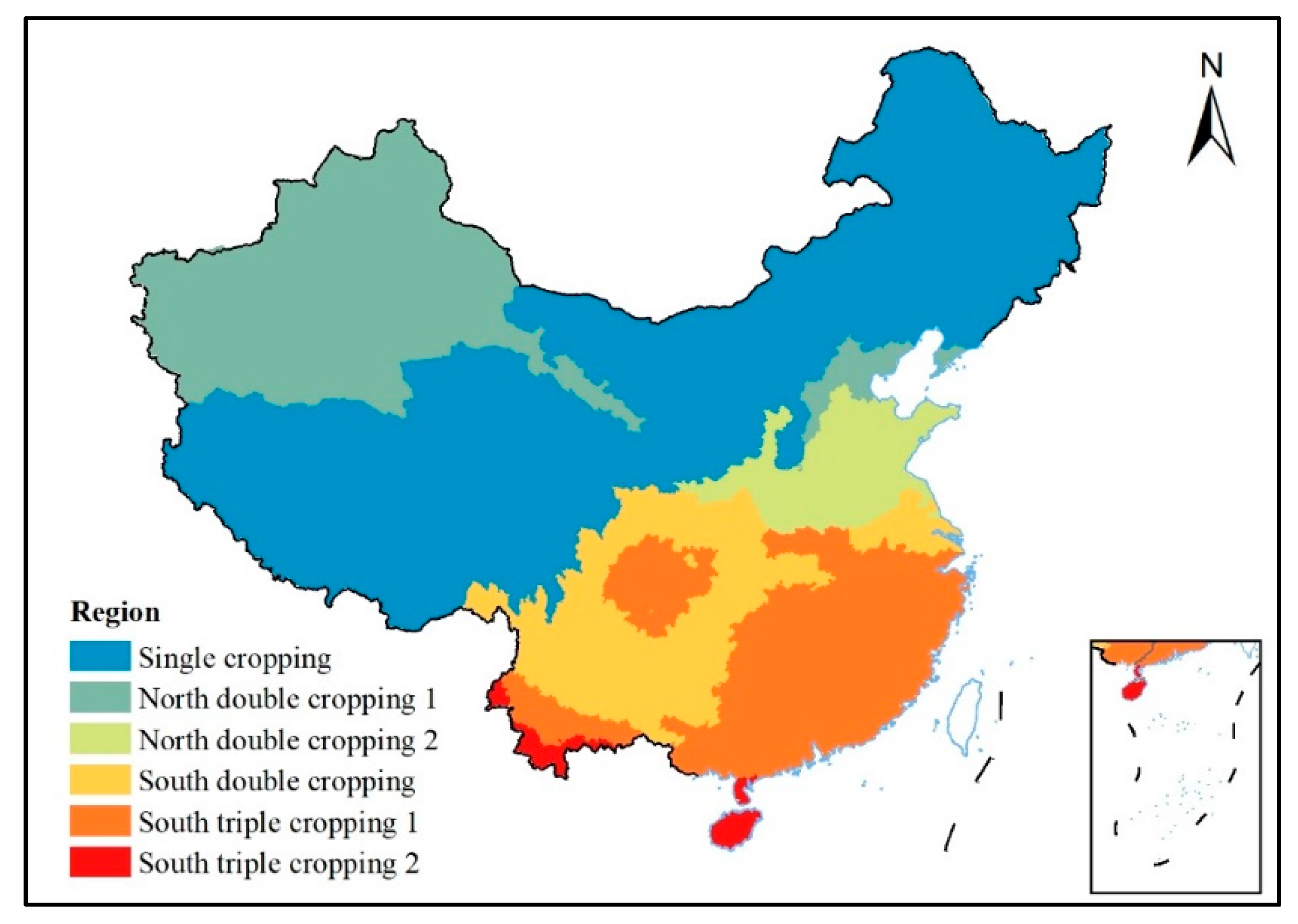
Figure 1. Distribution of the six agricultural regions with different cropping patterns in China.
Remotesensing 14 01800 g001
Figure 2. Workflow schematic for mapping crop distribution based on remote-sensing-derived cropping seasons and a regional crop calendar. Note: EVI, enhanced vegetation index; HANTS, harmonic analysis of time series.
Remotesensing 14 01800 g002
Figure 3. Time series profile curves of the vegetation index in regions where double cropping could potentially be applied, though it is not necessarily applied (a,b) and in regions where triple cropping could potentially be applied, though it is not necessarily applied (cf). Curves with green dots are the major patterns considered in this study. The curves with yellow dots in (a,c) indicate the presence of a single cropping pattern, but these patterns were not the majority and so were not separated from the majority type presented by green dots. We named these patterns as follows: pattern 2-1 (a), pattern 2-2 (b), pattern 3-1 (c), pattern 3-2 (d), pattern 3-3 (e), and pattern 3-4 (f). Consistent with Zuo et al. (2013), we avoided false peaks by discarding data obtained after 320 Julian day, which was especially helpful when winter wheat was planted.
Remotesensing 14 01800 g003
Figure 4. Comparison of remote sensing results with statistical data. WCD: winter crops in potentially double cropped areas; WCT: winter crops in potentially triple cropped areas; MCT: main season crops in triple cropped areas. (ac): comparison at the county level for the whole country; (df): plots of fitness, represented by R2, against the percent of harvest areas of the crops of concern at the province level; (gi): comparisons at the county level for the first four provinces with the highest harvest areas of the crops of concern.
Remotesensing 14 01800 g004
Figure 5. Comparison of rice area from our results and paddy fields extracted from the NLCD-C.
Remotesensing 14 01800 g005
Figure 6. Comparison of the results from the allocation model based on cropping patterns (a) and the results from the average allocation model (b). Counties were randomly chosen from those with high harvest areas: wheat in Xintai County, the Huang-Huai-Hai region; soybean in Jincheng County, the Loess Plateau; rapeseed in Xuncheng County, the Yangtze River Middle and Lower Plain; potato in Ankang County, the southwest region; maize in Renshou County, the southwest region; rice in Fengcheng County, the Yangtze River Middle and Lower Plain; and sugarcane in Shule County, the Southern China region.
Remotesensing 14 01800 g006
Figure 7. Comparison of the variation in SHDI between the results from our model and those from the average allocation model for each crop.
Remotesensing 14 01800 g007
Figure 8. Spatial distribution of the 14 studied crops (including three varieties for rice and two for wheat) in 2015.
Remotesensing 14 01800 g008
Figure 9. Spatial patterns of area change for wheat, rice, soybean, and maize from 2000 to 2015.
Remotesensing 14 01800 g009
Table 1. Cropping patterns in the six agricultural regions.
RegionsCropping Patterns
Winter CropsCrops in Main Season
Single Cropped TypesDouble Cropped TypesTriple Cropped Types
Single cropping areaAll crops
North double cropping area 1Winter wheatSpring wheat, Cotton, Barley, Millet, Sorghum, Sugarbeet, Soybean, Potato, Groundnut, Maize, SunflowerMiddle rice, Maize, Sunflower
North double cropping area 2Winter wheat, RapeseedSpring wheat, Barley, Millet, Sugarbeet, Middle rice, Potato, Sorghum, Maize, Soybean, SunflowerCotton, Groundnut, Maize, Soybean, Sunflower
South double cropping areaWinter wheat, Rapeseed Sugarcane, Groundnut, Maize, PotatoSoybean, Sunflower, Sorghum, Cotton, Middle rice, Early rice, Late rice, Groundnut, Maize, Potato
South triple cropping area 1Winter wheat, Rapeseed, BarleySugarcaneSunflower, Sorghum, Soybean, Middle rice, PotatoMaize, Early rice, Late rice, Groundnut, Soybean, Middle rice, Potato
South triple cropping area 2Winter wheat, Rapeseed, Potato, SoybeanSugarcaneCotton, Sunflower, SorghumMaize, Groundnut, Early rice, Late rice, Middle rice, Soybean
Publisher’s Note: MDPI stays neutral with regard to jurisdictional claims in published maps and institutional affiliations.