
Spatiotemporal Reconstruction of MODIS Normalized Difference Snow Index Products Using U-Net with Partial Convolutions


Abstract
:
1. Introduction
2. Study Area and Data
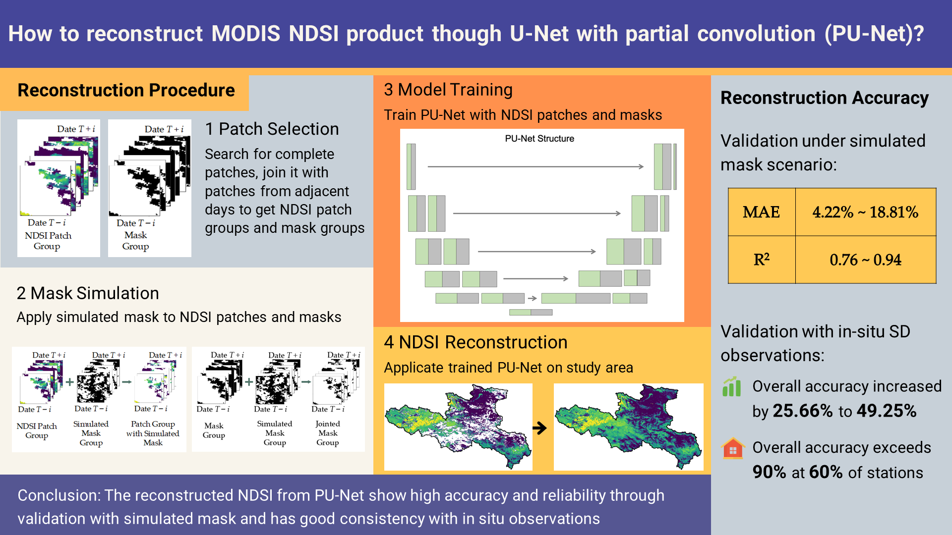
2.1. Study Area
2.2. Data
2.2.1. MODIS C6 Snow Cover Products
2.2.2. Meteorological Snow Depth (SD) Data
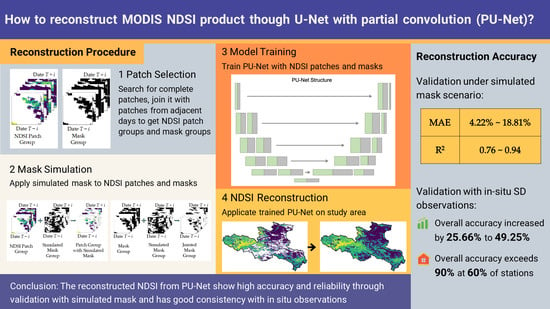
3. Methodology
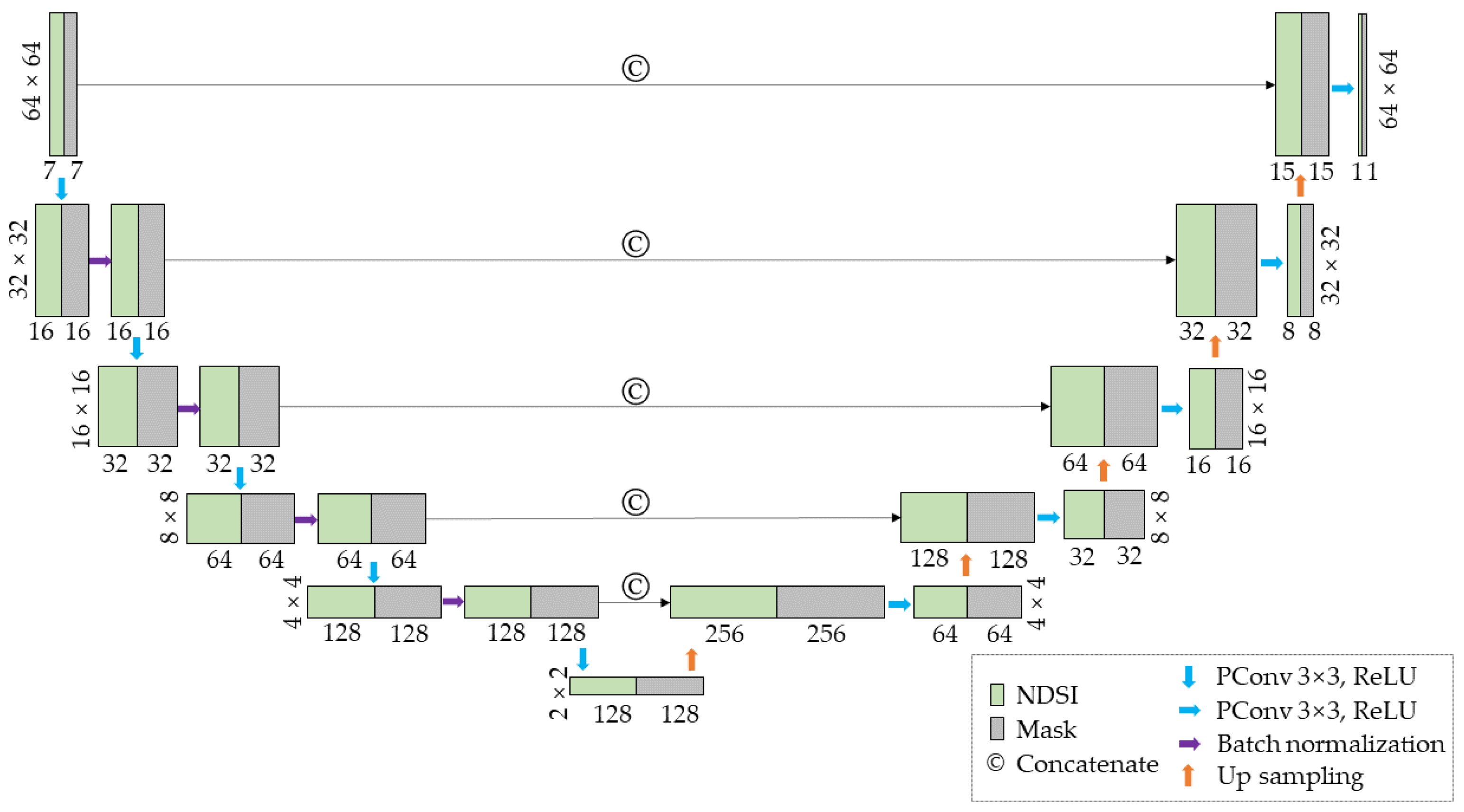
3.1. U-Net
3.2. Partial Convolution
3.3. MODIS NDSI Gap-Filling Framework Based on PU-Net
3.3.1. Preprocessing for Gap-Filling
3.3.2. Gap-Filling Framework

3.4. Model Training and Application
3.5. Validation Methodology
3.5.1. Simulated Cloud Mask
3.5.2. Validation with In-Situ SD Observation
4. Experiment Results
4.1. Visual Results of Reconstruction
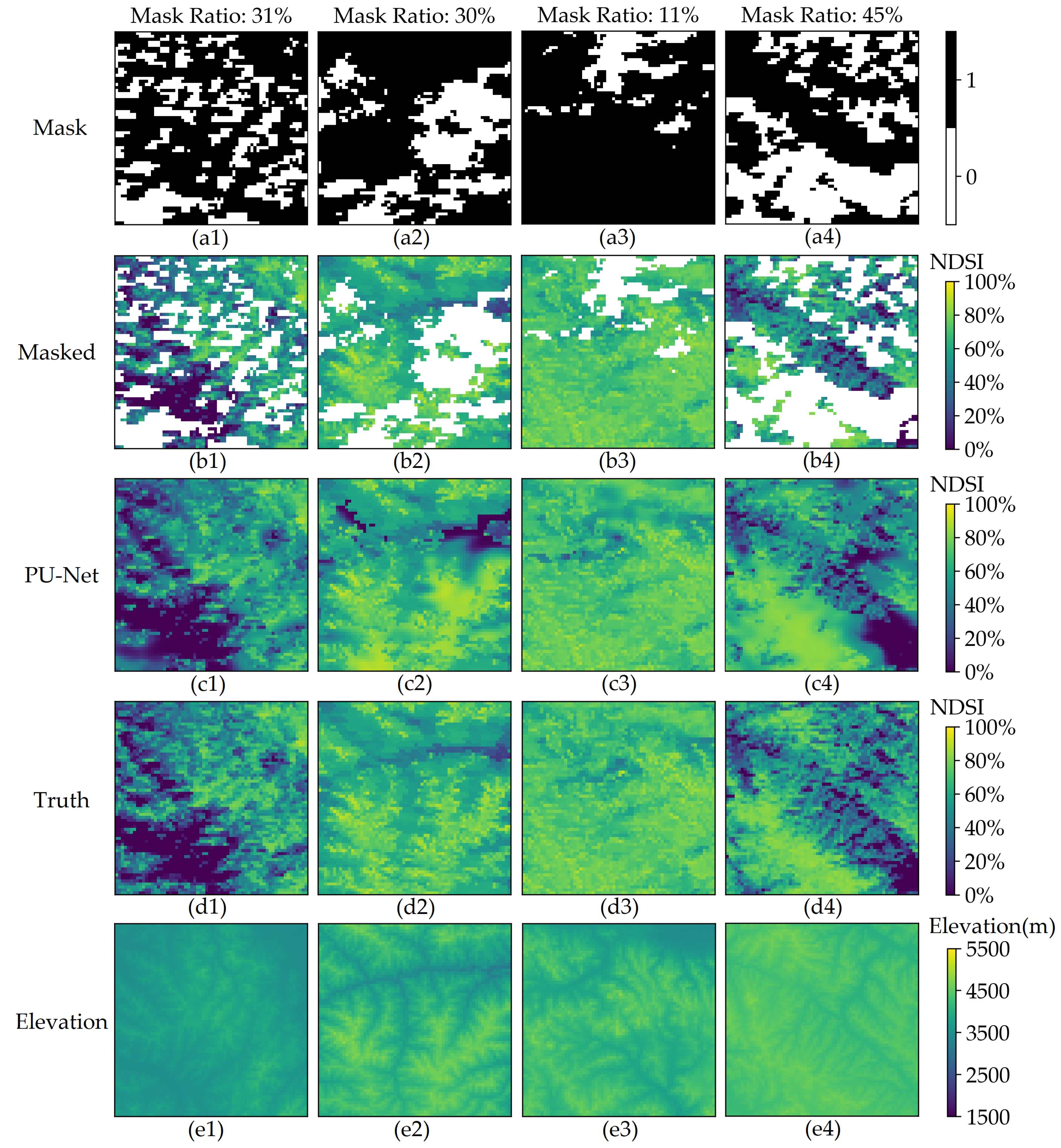
4.1.1. Results on Patches
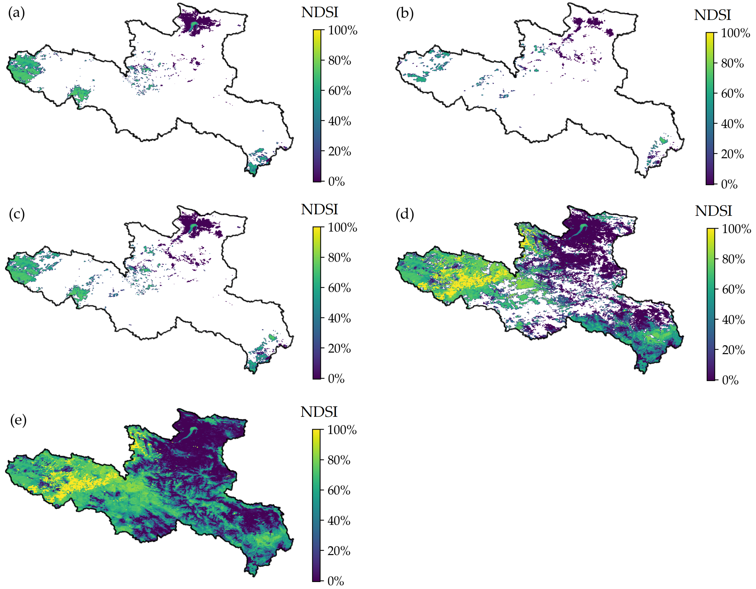
4.1.2. Results on Study Area
4.2. Validation with Simulated Mask
4.2.1. Validation on Patches
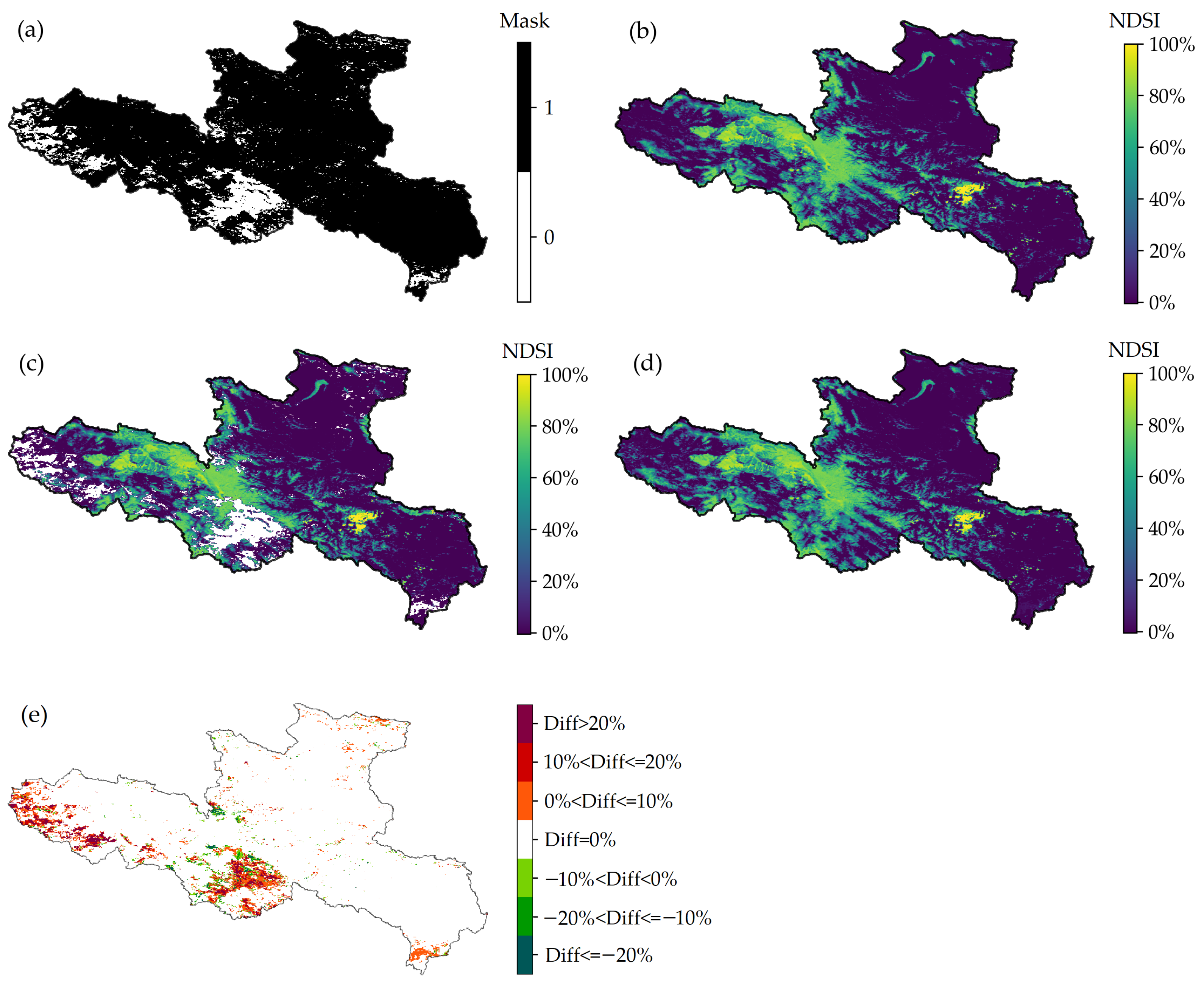
4.2.2. Validation on Entire Study Area
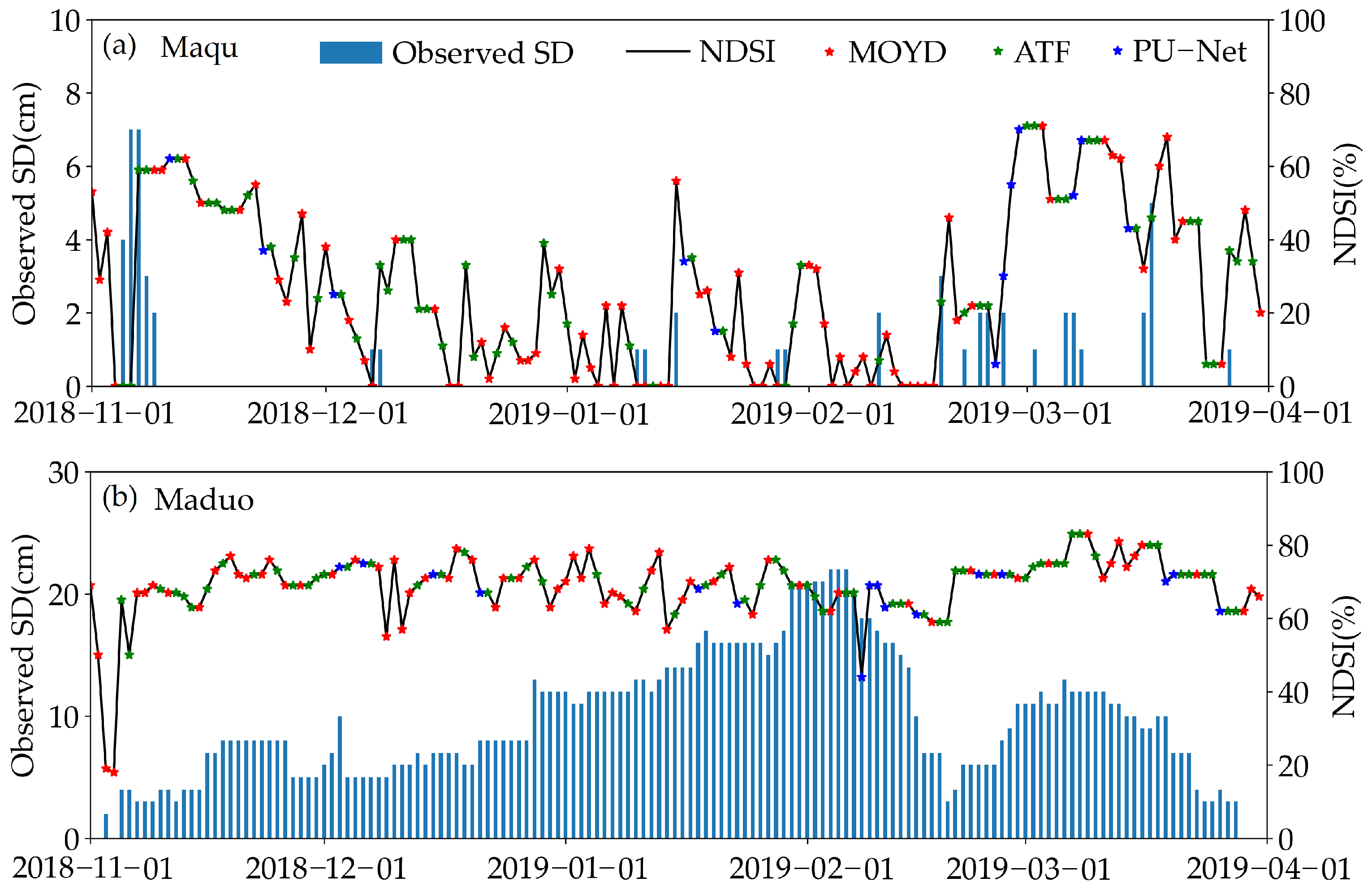
4.3. Validation with In Situ SD Observation
5. Discussion
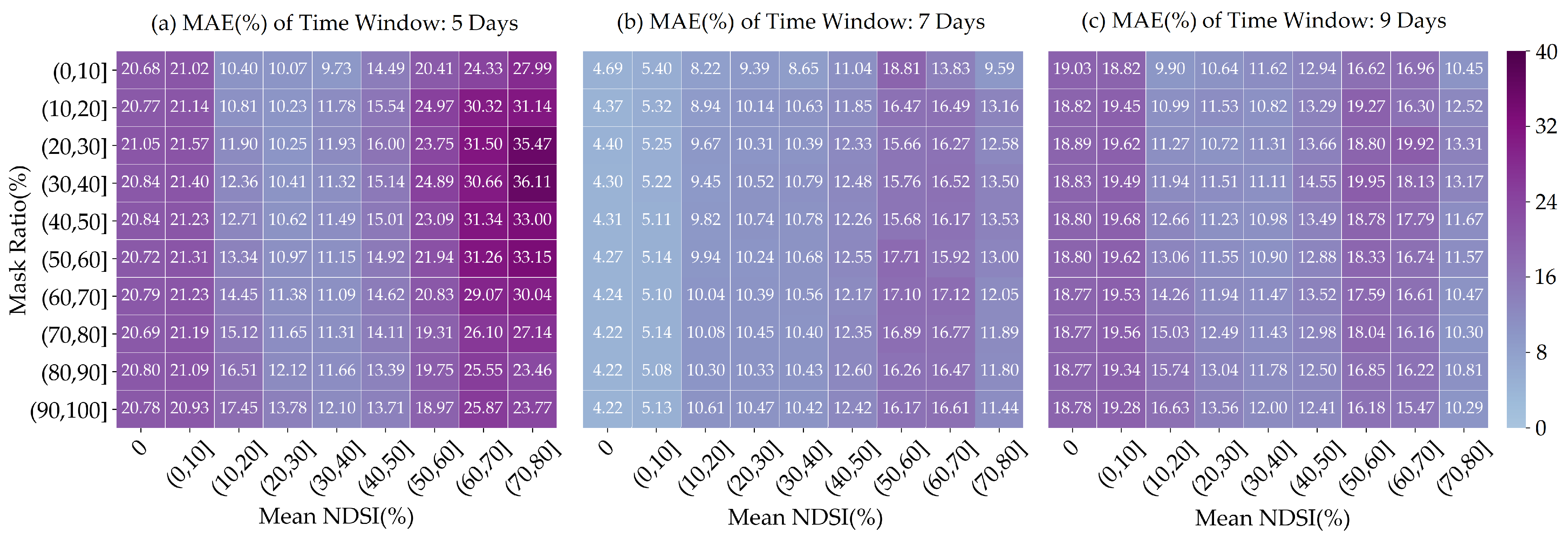
5.1. The Impact of Time Window on Reconstruction Accuracy
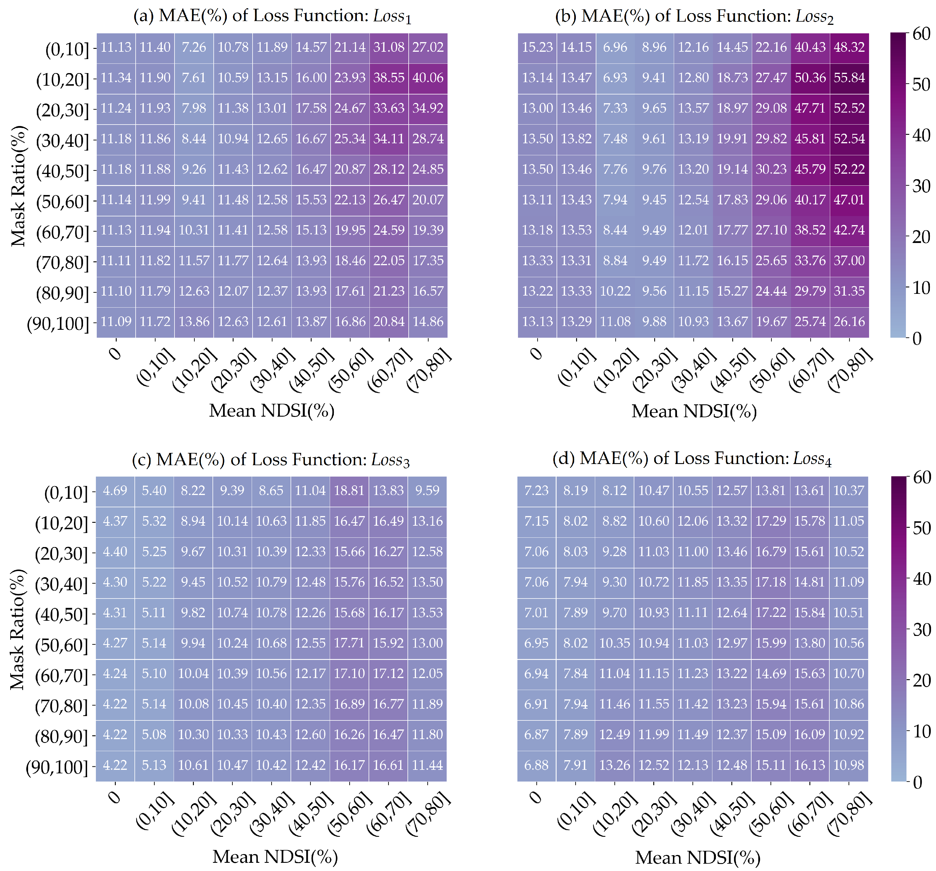
5.2. The Impact of Loss Function on Reconstruction Accuracy
- : L1 penalty with mask boundary loss;
- : L1 penalty without mask boundary loss;
- : L2 penalty with mask boundary loss;
- : L2 penalty without mask boundary loss.
6. Conclusions
Author Contributions
Funding
Data Availability Statement
Acknowledgments
Conflicts of Interest
References
- Dietz, A.J.; Kuenzer, C.; Gessner, U.; Dech, S. Remote sensing of snow—A review of available methods. Int. J. Remote Sens. 2012, 33, 4094–4134. [Google Scholar] [CrossRef]
- Robinson, D.A.; Dewey, K.F.; Heim, R.R., Jr. Global snow cover monitoring: An update. Bull. Am. Meteorol. Soc. 1993, 74, 1689–1696. [Google Scholar] [CrossRef] [Green Version]
- Brown, R.D. Northern Hemisphere snow cover variability and change, 1915–1997. J. Clim. 2000, 13, 2339–2355. [Google Scholar] [CrossRef]
- Brown, R.D.; Mote, P.W. The response of Northern Hemisphere snow cover to a changing climate. J. Clim. 2009, 22, 2124–2145. [Google Scholar] [CrossRef]
- Robock, A. The seasonal cycle of snow cover, sea ice and surface albedo. Mon. Weather. Rev. 1980, 108, 267–285. [Google Scholar] [CrossRef]
- Barnett, T.P.; Adam, J.C.; Lettenmaier, D.P. Potential impacts of a warming climate on water availability in snow-dominated regions. Nature 2005, 438, 303–309. [Google Scholar] [CrossRef]
- Wang, W.; Liang, T.; Huang, X.; Feng, Q.; Xie, H.; Liu, X.; Chen, M.; Wang, X. Early warning of snow-caused disasters in pastoral areas on the Tibetan Plateau. Nat. Hazards Earth Syst. Sci. 2013, 13, 1411–1425. [Google Scholar] [CrossRef]
- Mijinyawa, Y.; Dlamini, S.S. Impact Assessment of Water Scarcity at Somntongo in the Lowveld Region of Swaziland. Sci. Res. Essays 2008, 3, 61. [Google Scholar]
- Hall, D. Remote Sensing of Ice and Snow; Springer Science & Business Media: Berlin/Heidelberg, Germany, 2012. [Google Scholar]
- Hall, D.K.; Riggs, G.A.; Salomonson, V.V.; DiGirolamo, N.E.; Bayr, K.J. MODIS snow-cover products. Remote Sens. Environ. 2002, 83, 181–194. [Google Scholar] [CrossRef] [Green Version]
- Hall, D.K.; Riggs, G.A. Accuracy assessment of the MODIS snow products. Hydrol. Process. Int. J. 2007, 21, 1534–1547. [Google Scholar] [CrossRef]
- Parajka, J.; Blöschl, G. Validation of MODIS snow cover images over Austria. Hydrol. Earth Syst. Sci. 2006, 10, 679–689. [Google Scholar] [CrossRef] [Green Version]
- Huang, X.; Liang, T.; Zhang, X.; Guo, Z. Validation of MODIS snow cover products using Landsat and ground measurements during the 2001–2005 snow seasons over northern Xinjiang, China. Int. J. Remote Sens. 2011, 32, 133–152. [Google Scholar] [CrossRef]
- Klein, A.G.; Barnett, A.C. Validation of daily MODIS snow cover maps of the Upper Rio Grande River Basin for the 2000–2001 snow year. Remote Sens. Environ. 2003, 86, 162–176. [Google Scholar] [CrossRef]
- Flueraru, C.; Stancalie, G.; Craciunescu, V.; Savin, E. A validation of MODIS snowcover products in Romania: Challenges and future directions. Trans. GIS 2007, 11, 927–941. [Google Scholar] [CrossRef]
- Ciancia, E.; Coviello, I.; Di Polito, C.; Lacava, T.; Pergola, N.; Satriano, V.; Tramutoli, V. Investigating the chlorophyll-a variability in the Gulf of Taranto (North-western Ionian Sea) by a multi-temporal analysis of MODIS-Aqua Level 3/Level 2 data. Cont. Shelf Res. 2018, 155, 34–44. [Google Scholar] [CrossRef]
- Li, X.; Shen, H.; Zhang, L.; Zhang, H.; Yuan, Q.; Yang, G. Recovering quantitative remote sensing products contaminated by thick clouds and shadows using multitemporal dictionary learning. IEEE Trans. Geosci. Remote Sens. 2014, 52, 7086–7098. [Google Scholar]
- Li, X.; Jing, Y.; Shen, H.; Zhang, L. The recent developments in cloud removal approaches of MODIS snow cover product. Hydrol. Earth Syst. Sci. 2019, 23, 2401–2416. [Google Scholar] [CrossRef] [Green Version]
- Tong, J.; Déry, S.; Jackson, P. Topographic control of snow distribution in an alpine watershed of western Canada inferred from spatially-filtered MODIS snow products. Hydrol. Earth Syst. Sci. 2009, 13, 319–326. [Google Scholar] [CrossRef] [Green Version]
- Parajka, J.; Pepe, M.; Rampini, A.; Rossi, S.; Blöschl, G. A regional snow-line method for estimating snow cover from MODIS during cloud cover. J. Hydrol. 2010, 381, 203–212. [Google Scholar] [CrossRef]
- López-Burgos, V.; Gupta, H.V.; Clark, M. Reducing cloud obscuration of MODIS snow cover area products by combining spatio-temporal techniques with a probability of snow approach. Hydrol. Earth Syst. Sci. 2013, 17, 1809–1823. [Google Scholar] [CrossRef] [Green Version]
- Jing, Y.; Shen, H.; Li, X.; Guan, X. A two-stage fusion framework to generate a spatio–temporally continuous MODIS NDSI product over the Tibetan Plateau. Remote Sens. 2019, 11, 2261. [Google Scholar] [CrossRef] [Green Version]
- Parajka, J.; Blöschl, G. Spatio-temporal combination of MODIS images–potential for snow cover mapping. Water Resour. Res. 2008, 44, 1–13. [Google Scholar] [CrossRef]
- Chen, S.; Yang, Q.; Xie, H.; Zhang, H.; Lu, P.; Zhou, C. Spatiotemporal variations of snow cover in northeast China based on flexible multiday combinations of moderate resolution imaging spectroradiometer snow cover products. J. Appl. Remote Sens. 2014, 8, 084685. [Google Scholar] [CrossRef]
- Paudel, K.P.; Andersen, P. Monitoring snow cover variability in an agropastoral area in the Trans Himalayan region of Nepal using MODIS data with improved cloud removal methodology. Remote Sens. Environ. 2011, 115, 1234–1246. [Google Scholar] [CrossRef]
- Wang, X.; Zheng, H.; Chen, Y.; Liu, H.; Liu, L.; Huang, H.; Liu, K. Mapping snow cover variations using a MODIS daily cloud-free snow cover product in northeast China. J. Appl. Remote Sens. 2014, 8, 084681. [Google Scholar] [CrossRef] [Green Version]
- Gao, Y.; Xie, H.; Yao, T.; Xue, C. Integrated assessment on multi-temporal and multi-sensor combinations for reducing cloud obscuration of MODIS snow cover products of the Pacific Northwest USA. Remote Sens. Environ. 2010, 114, 1662–1675. [Google Scholar] [CrossRef]
- Hou, J.; Huang, C.; Zhang, Y.; Guo, J.; Gu, J. Gap-filling of modis fractional snow cover products via non-local spatio-temporal filtering based on machine learning techniques. Remote Sens. 2019, 11, 90. [Google Scholar] [CrossRef] [Green Version]
- Li, M.; Zhu, X.; Li, N.; Pan, Y. Gap-Filling of a MODIS Normalized Difference Snow Index Product Based on the Similar Pixel Selecting Algorithm: A Case Study on the Qinghai–Tibetan Plateau. Remote Sens. 2020, 12, 1077. [Google Scholar] [CrossRef] [Green Version]
- Wang, X.; Xie, H.; Liang, T.; Huang, X. Comparison and validation of MODIS standard and new combination of Terra and Aqua snow cover products in northern Xinjiang, China. Hydrol. Process. Int. J. 2009, 23, 419–429. [Google Scholar] [CrossRef]
- Chen, S.; Wang, X.; Guo, H.; Xie, P.; Sirelkhatim, A.M. Spatial and temporal adaptive gap-filling method producing daily cloud-free ndsi time series. IEEE J. Sel. Top. Appl. Earth Obs. Remote Sens. 2020, 13, 2251–2263. [Google Scholar] [CrossRef]
- Liu, G.; Reda, F.A.; Shih, K.J.; Wang, T.C.; Tao, A.; Catanzaro, B. Image inpainting for irregular holes using partial convolutions. In Proceedings of the European Conference on Computer Vision (ECCV), Munich, Germany, 8–14 September 2018; pp. 85–100. [Google Scholar]
- Zhang, Q.; Yuan, Q.; Li, J.; Wang, Y.; Sun, F.; Zhang, L. Generating seamless global daily AMSR2 soil moisture (SGD-SM) long-term products for the years 2013–2019. Earth Syst. Sci. Data 2021, 13, 1385–1401. [Google Scholar] [CrossRef]
- Wu, P.; Yin, Z.; Yang, H.; Wu, Y.; Ma, X. Reconstructing geostationary satellite land surface temperature imagery based on a multiscale feature connected convolutional neural network. Remote Sens. 2019, 11, 300. [Google Scholar] [CrossRef] [Green Version]
- Yu, J.; Lin, Z.; Yang, J.; Shen, X.; Lu, X.; Huang, T.S. Generative image inpainting with contextual attention. In Proceedings of the IEEE Conference on Computer Vision and Pattern Recognition, Salt Lake City, UT, USA, 18–23 June 2018; pp. 5505–5514. [Google Scholar]
- Russakovsky, O.; Deng, J.; Su, H.; Krause, J.; Satheesh, S.; Ma, S.; Huang, Z.; Karpathy, A.; Khosla, A.; Bernstein, M.; et al. Imagenet large scale visual recognition challenge. Int. J. Comput. Vis. 2015, 115, 211–252. [Google Scholar] [CrossRef] [Green Version]
- Song, Y.; Yang, C.; Lin, Z.; Liu, X.; Huang, Q.; Li, H.; Kuo, C.C.J. Contextual-based image inpainting: Infer, match, and translate. In Proceedings of the European Conference on Computer Vision (ECCV), Munich, Germany, 8–14 September 2018; pp. 3–19. [Google Scholar]
- Liu, X.; Chen, B. Climatic warming in the Tibetan Plateau during recent decades. Int. J. Climatol. J. R. Meteorol. Soc. 2000, 20, 1729–1742. [Google Scholar] [CrossRef]
- Ye, D.; Gao, Y. The Meteorology of the Qinghai-Xizang (Tibet) Plateau; Science Press: Beijing, China, 1979; pp. 1–278. (In Chinese) [Google Scholar]
- Yanai, M.; Li, C.; Song, Z. Seasonal heating of the Tibetan Plateau and its effects on the evolution of the Asian summer monsoon. J. Meteorol. Soc. Jpn. Ser. II 1992, 70, 319–351. [Google Scholar] [CrossRef] [Green Version]
- Kutzbach, J.; Prell, W.; Ruddiman, W.F. Sensitivity of Eurasian climate to surface uplift of the Tibetan Plateau. J. Geol. 1993, 101, 177–190. [Google Scholar] [CrossRef]
- Zheng, H.; Zhang, L.; Liu, C.; Shao, Q.; Fukushima, Y. Changes in stream flow regime in headwater catchments of the Yellow River basin since the 1950s. Hydrol. Process. Int. J. 2007, 21, 886–893. [Google Scholar] [CrossRef]
- Sato, Y.; Ma, X.; Xu, J.; Matsuoka, M.; Zheng, H.; Liu, C.; Fukushima, Y. Analysis of long-term water balance in the source area of the Yellow River basin. Hydrol. Process. Int. J. 2008, 22, 1618–1629. [Google Scholar] [CrossRef]
- Qin, Y.; Yang, D.; Gao, B.; Wang, T.; Chen, J.; Chen, Y.; Wang, Y.; Zheng, G. Impacts of climate warming on the frozen ground and eco-hydrology in the Yellow River source region, China. Sci. Total Environ. 2017, 605, 830–841. [Google Scholar] [CrossRef] [Green Version]
- Li, C.; Su, F.; Yang, D.; Tong, K.; Meng, F.; Kan, B. Spatiotemporal variation of snow cover over the Tibetan Plateau based on MODIS snow product, 2001–2014. Int. J. Climatol. 2018, 38, 708–728. [Google Scholar] [CrossRef]
- Hu, Y.; Maskey, S.; Uhlenbrook, S. Trends in temperature and rainfall extremes in the Yellow River source region, China. Clim. Change 2012, 110, 403–429. [Google Scholar] [CrossRef] [Green Version]
- Ronneberger, O.; Fischer, P.; Brox, T. U-net: Convolutional networks for biomedical image segmentation. In International Conference on Medical Image Computing and Computer-Assisted Intervention; Springer: Berlin/Heidelberg, Germany, 2015; pp. 234–241. [Google Scholar]
- Zhang, Q.; Yuan, Q.; Li, J.; Yang, Z.; Ma, X. Learning a dilated residual network for SAR image despeckling. Remote Sens. 2018, 10, 196. [Google Scholar] [CrossRef] [Green Version]
- Yang, J.; Jiang, L.; Ménard, C.B.; Luojus, K.; Lemmetyinen, J.; Pulliainen, J. Evaluation of snow products over the Tibetan Plateau. Hydrol. Process. 2015, 29, 3247–3260. [Google Scholar] [CrossRef]
- Gao, Y.; Xie, H.; Yao, T. Developing snow cover parameters maps from MODIS, AMSR-E, and blended snow products. Photogramm. Eng. Remote Sens. 2011, 77, 351–361. [Google Scholar] [CrossRef]
- Albawi, S.; Mohammed, T.A.; Al-Zawi, S. Understanding of a convolutional neural network. In Proceedings of the 2017 International Conference on Engineering and Technology (ICET), Antalya, Turkey, 21–23 August 2017; pp. 1–6. [Google Scholar]
- Schmidt, R.M.; Schneider, F.; Hennig, P. Descending through a crowded valley-benchmarking deep learning optimizers. In Proceedings of the International Conference on Machine Learning, Virtual Event, 18–24 July 2021; pp. 9367–9376. [Google Scholar]
- Li, Z.; Liu, F.; Yang, W.; Peng, S.; Zhou, J. A survey of convolutional neural networks: Analysis, applications, and prospects. IEEE Trans. Neural Netw. Learn. Syst. 2021, 1, 1–21. [Google Scholar] [CrossRef]
- Bernico, M. Deep Learning Quick Reference: Useful Hacks for Training and Optimizing Deep Neural Networks with TensorFlow and Keras; Packt Publishing Ltd.: Birmingham, UK, 2018. [Google Scholar]
- Wilks, D.S. Statistical Methods in the Atmospheric Sciences; Academic Press: Cambridge, MA, USA, 2011; Volume 100. [Google Scholar]
- Lee, C.S.; Sohn, E.; Park, J.D.; Jang, J.D. Estimation of soil moisture using deep learning based on satellite data: A case study of South Korea. GISci. Remote Sens. 2019, 56, 43–67. [Google Scholar] [CrossRef]


| Observed SD | |||
|---|---|---|---|
| No Snow (< cm) | Snow ( cm) | ||
| No Snow (<) | a | b | |
| MODIS NDSI | Snow() | c | d |
| Cloud | e | f | |
| MAE (%) | Mean NDSI (%) | |||||||||
|---|---|---|---|---|---|---|---|---|---|---|
| 0 | (0, 10] | (10, 20] | (20, 30] | (30, 40] | (40, 50] | (50, 60] | (60, 70] | (70, 80] | ||
| (0, 10] | 4.69 | 5.40 | 8.22 | 9.39 | 8.65 | 11.04 | 18.81 | 13.83 | 9.59 | |
| (10, 20] | 4.37 | 5.32 | 8.94 | 10.14 | 10.63 | 11.85 | 16.47 | 16.49 | 13.16 | |
| (20, 30] | 4.40 | 5.25 | 9.67 | 10.31 | 10.39 | 12.33 | 15.66 | 16.27 | 12.58 | |
| (30, 40] | 4.30 | 5.22 | 9.45 | 10.52 | 10.79 | 12.48 | 15.76 | 16.52 | 13.50 | |
| Mask Ratio (%) | (40, 50] | 4.31 | 5.11 | 9.82 | 10.74 | 10.78 | 12.26 | 15.68 | 16.17 | 13.53 |
| (50, 60] | 4.27 | 5.14 | 9.94 | 10.24 | 10.68 | 12.55 | 17.71 | 15.92 | 13.00 | |
| (60, 70] | 4.24 | 5.10 | 10.04 | 10.39 | 10.56 | 12.17 | 17.10 | 17.12 | 12.05 | |
| (70, 80] | 4.22 | 5.14 | 10.08 | 10.45 | 10.40 | 12.35 | 16.89 | 16.77 | 11.89 | |
| (80, 90] | 4.22 | 5.08 | 10.30 | 10.33 | 10.43 | 12.60 | 16.26 | 16.47 | 11.80 | |
| (90, 100] | 4.22 | 5.13 | 10.61 | 10.47 | 10.42 | 12.42 | 16.17 | 16.61 | 11.44 | |
| R | Mean NDSI (%) | ||||||||
|---|---|---|---|---|---|---|---|---|---|
| (0, 10] | (10, 20] | (20, 30] | (30, 40] | (40, 50] | (50, 60] | (60, 70] | (70, 80] | ||
| (0, 10] | 0.92 | 0.90 | 0.88 | 0.91 | 0.85 | 0.76 | 0.82 | 0.90 | |
| (10, 20] | 0.94 | 0.89 | 0.86 | 0.86 | 0.84 | 0.77 | 0.78 | 0.83 | |
| (20, 30] | 0.92 | 0.89 | 0.87 | 0.86 | 0.84 | 0.79 | 0.78 | 0.84 | |
| (30, 40] | 0.92 | 0.89 | 0.86 | 0.87 | 0.84 | 0.80 | 0.78 | 0.83 | |
| Mask Ratio (%) | (40, 50] | 0.92 | 0.89 | 0.88 | 0.88 | 0.83 | 0.79 | 0.78 | 0.82 |
| (50, 60] | 0.91 | 0.88 | 0.87 | 0.87 | 0.82 | 0.78 | 0.78 | 0.81 | |
| (60, 70] | 0.92 | 0.88 | 0.87 | 0.88 | 0.83 | 0.80 | 0.77 | 0.84 | |
| (70, 80] | 0.91 | 0.89 | 0.88 | 0.88 | 0.83 | 0.80 | 0.77 | 0.85 | |
| (80, 90] | 0.91 | 0.88 | 0.88 | 0.87 | 0.83 | 0.78 | 0.78 | 0.87 | |
| (90, 100] | 0.91 | 0.88 | 0.87 | 0.88 | 0.84 | 0.79 | 0.78 | 0.87 | |
| MAE (%) | MODIS NDSI Date | |||
|---|---|---|---|---|
| 10 October 2018 | 29 November 2018 | 30 March 2019 | ||
| 10 October 2017 | 12.906 | - | - | |
| Mask Date | 29 November 2017 | - | 14.369 | - |
| 30 March 2018 | - | - | 12.106 | |
| R | MODIS NDSI Date | |||
|---|---|---|---|---|
| 10 October 2018 | 29 November 2018 | 30 March 2019 | ||
| 10 October 2017 | 0. 844 | - | - | |
| Mask Date | 29 November 2017 | - | 0. 813 | - |
| 30 March 2018 | - | - | 0.851 | |
| MODIS NDSI | |||||||||
|---|---|---|---|---|---|---|---|---|---|
| MOYD | ATF | PU-Net | |||||||
| Site | OA (%) | MU (%) | MO (%) | OA (%) | MU (%) | MO (%) | OA (%) | MU (%) | MO (%) |
| Gonghe | 55.63 | 1.10 | 6.59 | 88.32 | 3.79 | 4.55 | 91.30 | 4.35 | 4.35 |
| Guide | 70.86 | 0.00 | 0.93 | 96.62 | 0.00 | 0.69 | 99.32 | 0.00 | 0.68 |
| Xinghai | 62.91 | 0.94 | 9.43 | 87.77 | 4.35 | 7.25 | 88.57 | 4.29 | 7.14 |
| Maduo | 43.71 | 0.00 | 7.04 | 84.62 | 0.00 | 7.04 | 92.96 | 0.00 | 7.04 |
| Dari | 41.06 | 7.32 | 17.07 | 73.28 | 11.29 | 11.29 | 76.56 | 12.50 | 10.94 |
| Henan | 62.91 | 2.86 | 6.67 | 89.78 | 4.41 | 5.15 | 90.44 | 4.41 | 5.15 |
| Jiuzhi | 49.01 | 5.68 | 10.23 | 79.70 | 7.26 | 7.26 | 85.04 | 7.87 | 7.09 |
| Maqu | 39.74 | 0.00 | 28.63 | 74.17 | 2.63 | 19.30 | 79.17 | 2.50 | 18.33 |
| Ruoergai | 65.56 | 2.88 | 1.92 | 88.41 | 5.34 | 1.53 | 92.59 | 5.93 | 1.48 |
| Hongyuan | 64.90 | 2.78 | 6.48 | 90.85 | 3.55 | 4.96 | 91.61 | 3.50 | 4.90 |
Publisher’s Note: MDPI stays neutral with regard to jurisdictional claims in published maps and institutional affiliations. |
© 2022 by the authors. Licensee MDPI, Basel, Switzerland. This article is an open access article distributed under the terms and conditions of the Creative Commons Attribution (CC BY) license (https://creativecommons.org/licenses/by/4.0/).
Share and Cite
Xing, D.; Hou, J.; Huang, C.; Zhang, W. Spatiotemporal Reconstruction of MODIS Normalized Difference Snow Index Products Using U-Net with Partial Convolutions. Remote Sens. 2022, 14, 1795. https://doi.org/10.3390/rs14081795
Xing D, Hou J, Huang C, Zhang W. Spatiotemporal Reconstruction of MODIS Normalized Difference Snow Index Products Using U-Net with Partial Convolutions. Remote Sensing. 2022; 14(8):1795. https://doi.org/10.3390/rs14081795
Chicago/Turabian StyleXing, De, Jinliang Hou, Chunlin Huang, and Weimin Zhang. 2022. "Spatiotemporal Reconstruction of MODIS Normalized Difference Snow Index Products Using U-Net with Partial Convolutions" Remote Sensing 14, no. 8: 1795. https://doi.org/10.3390/rs14081795
APA StyleXing, D., Hou, J., Huang, C., & Zhang, W. (2022). Spatiotemporal Reconstruction of MODIS Normalized Difference Snow Index Products Using U-Net with Partial Convolutions. Remote Sensing, 14(8), 1795. https://doi.org/10.3390/rs14081795