1. Introduction
The ocean environment has an important impact on human maritime operations. Having timely information about the current and future ocean environment is of great significance to ships that perform operations at sea. For ships on voyage, shipborne predictions that mean conducting variables predictions of ocean environment on board, are convenient approaches for obtaining marine information relative to receiving huge marine data from shore-based institutions.
In terms of ocean temperature, traditional methods of shipborne predictions are mainly based on statistical analysis of historical data, such as linear regression analysis-based prediction (LRAP). However, in general, traditional statistical methods cannot effectively capture the spatial characteristics of ocean data. Moreover, traditional statistical methods are not able to make effective use of observation data. This makes the prediction results generated through traditional statistical methods less accurate. Under the condition of shipborne predictions, using satellite remote sensing observations is an effective way to obtain more accurate ocean temperature. However, satellite remote sensing observations can only provide surface information and cannot directly provide subsurface information. Moreover, in this context, the acquired satellite remote sensing observations are delayed data points, and the real-time remote sensing information is hardly available. In order to address these issues, it is necessary to conduct information spatial-temporal extension (ISTE) of satellite remote sensing observations. As a result, four-dimensional (4D) prediction data can be generated from two-dimensional (2D) observation data and shipborne predictions driven by satellite remote sensing observations can be realized.
In fact, the information spatial extension (ISE) is equivalent to the spatial inversion of remote sensing data while the information temporal extension (ITE) is equivalent to the temporal prediction of remote sensing data. Previous studies have proposed various algorithms about ISE or ITE, which mainly include empirical analysis methods and artificial intelligence (AI) methods.
The algorithmic principle of Modular Ocean Data Assimilation System (MODAS) [
1] is a typical empirical analysis method for underwater inversion, which can effectively portray the underwater temperature structure using satellite remote sensing observations. With the rapid development of technology, AI represented by deep learning, has shown its strength in many scientific fields, which include geoscience [
2]. Subsequent researchers have attempted to use AI methods to perform underwater inversion. Ali et al. [
3] used artificial neural networks (ANNs) to estimate the subsurface temperature structures from surface variables. Lu et al. [
4] combined a pre-clustering process and a neural network to estimate the subsurface temperature anomaly using ocean surface variables at the global scale. Han et al. [
5] used a convolutional neural network (CNN) to estimate subsurface temperature from satellite remote sensing observations. Sammartino et al. [
6] proposed a Multi-Layer-Perceptron (MLP) network to reconstruct the three-dimensional (3D) fields of temperature.
It can be anticipated that the inversion accuracy will be improved using vertical observations in the inversion process, similar to studies carried out by Wang et al. [
7], which combined Argo profiles with satellite observations to reconstruct weekly three-dimensional temperature fields of the Pacific Ocean. In the situation of shipborne prediction, besides satellite remote sensing observations, it is convenient to obtain the ship survey observations. The ship survey observations data can provide subsurface vertical information. However, these observations are only distributed along the ship route. Meanwhile, the observation information of other locations is difficult to be obtained. In this context, using the limited ship survey observations to supplement the remote sensing observations with a suitable algorithm will further improve the prediction accuracy of the ocean environment.
Although previous studies have carried out research on the fusion of satellite remote sensing information and ocean observation vertical information, most of the vertical information comes from Argo grid data products, which means that these algorithms need enough vertical information data. In the situation of shipborne predictions, the vertical information data is limited along the ship route. For these special limited data, traditional methods with statistical analysis are difficult to fuse the ship survey observations and remote sensing observations [
8]. Therefore, a new scheme for data fusion that can make full use of limited ship survey observations is needed.
In order to obtain the future information of ocean environment, the ITE is required. Temporal intelligent prediction can be seen as an ITE algorithm of remote sensing observations, which can use AI methods to predict the future data. Neetu et al. [
9] proposed a nonlinear data-adaptive approach known by the name of genetic algorithm for predicting satellite-observed sea surface temperature (SST) in the Arabian Sea. Su et al. [
10] proposed a support vector machine approach that can estimate the subsurface temperature anomaly. Zhang et al. [
11] first adopts long short-term memory (LSTM) to predict SST. Xiao et al. [
12] proposed a machine learning method combining the LSTM deep recurrent neural network model and the AdaBoost ensemble learning model (LSTM-AdaBoost) to predict the short and mid-term daily SST. Wei et al. [
13] used ANNs to predict SST of the South China Sea. Sun et al. [
14] proposed a time-series graph network (TSGN) for SST prediction that can jointly capture graph-based spatial correlation and temporal dynamics. All these previous studies have developed various algorithms and achieved great success, which greatly promoted the development of ITE algorithms for remote sensing observations. However, for the temporal intelligent prediction of ocean temperature, most previous studies only focused on SST prediction [
9,
10,
11,
12,
13,
14,
15,
16,
17,
18,
19]. However, sea thermocline has a more important influence on the maritime operation, such as underwater navigation and hydroacoustic communication. A practical and effective prediction method should be applicable to the full range of water depths.
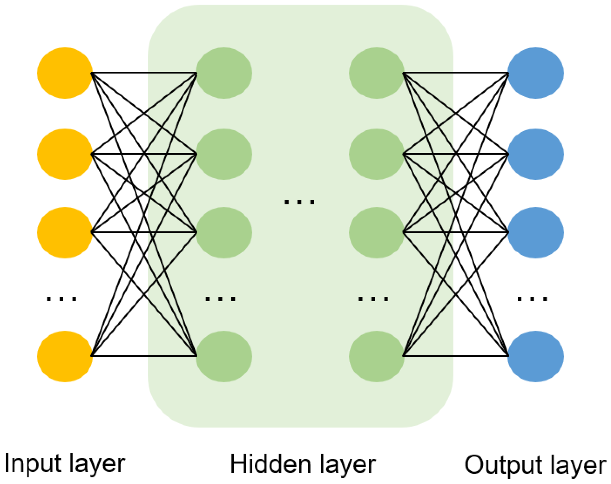
Deep learning, based on deep neural networks (DNNs), is a branch of machine learning. DNNs are ANNs structures with multiple layers, which can learn complex functions by combining nonlinear modules [
20,
21]. In geoscience, deep learning based on DNNs can better capture the spatial and temporal features of data that are difficult to extract by traditional methods with statistical analysis [
2,
22,
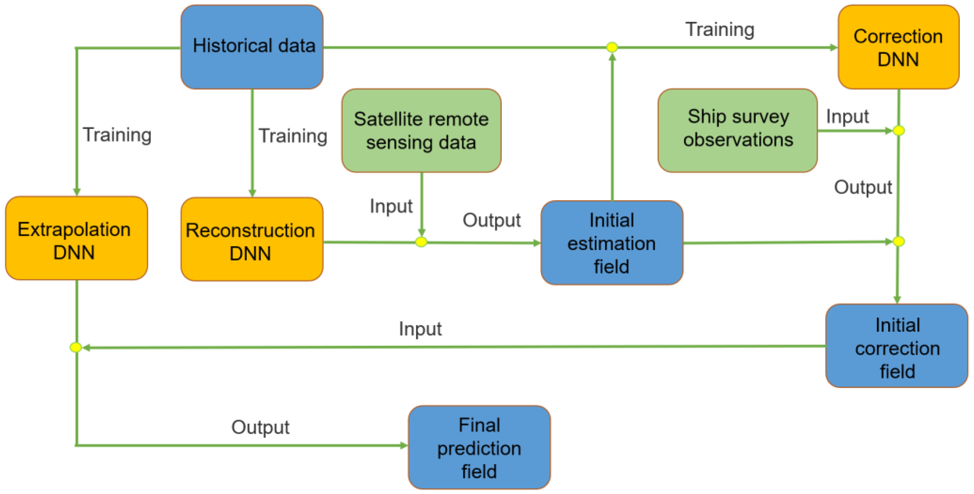
23]. To address the issues above, this study proposes an DNN-based ISTE algorithm for remote sensing SST. The ISTE algorithm can effectively fuse the satellite remote sensing SST data, ship survey observations data and historical data of ocean temperature to generate 4D ocean temperature prediction data. The main contributions of this study are as follows: (1) compared with previous studies, this study effectively integrate the limited ship survey observations using DNNs, which can improve the underwater inversion accuracy of satellite remote sensing SST; (2) this study uses DNNs to achieve temperature predictions over the full water depth, including the mixed layer, thermocline and deep layer; (3) the ISTE algorithm proposed in this study could be a new effective approach for shipborne predictions.
The remainder of this article is organized as follows.
Section 2 describes the ISTE principle and experimental details.
Section 3 presents the experimental results and performance evaluation of the ISTE. A discussion is given in
Section 4. Finally,
Section 5 summarizes this study.
3. Results
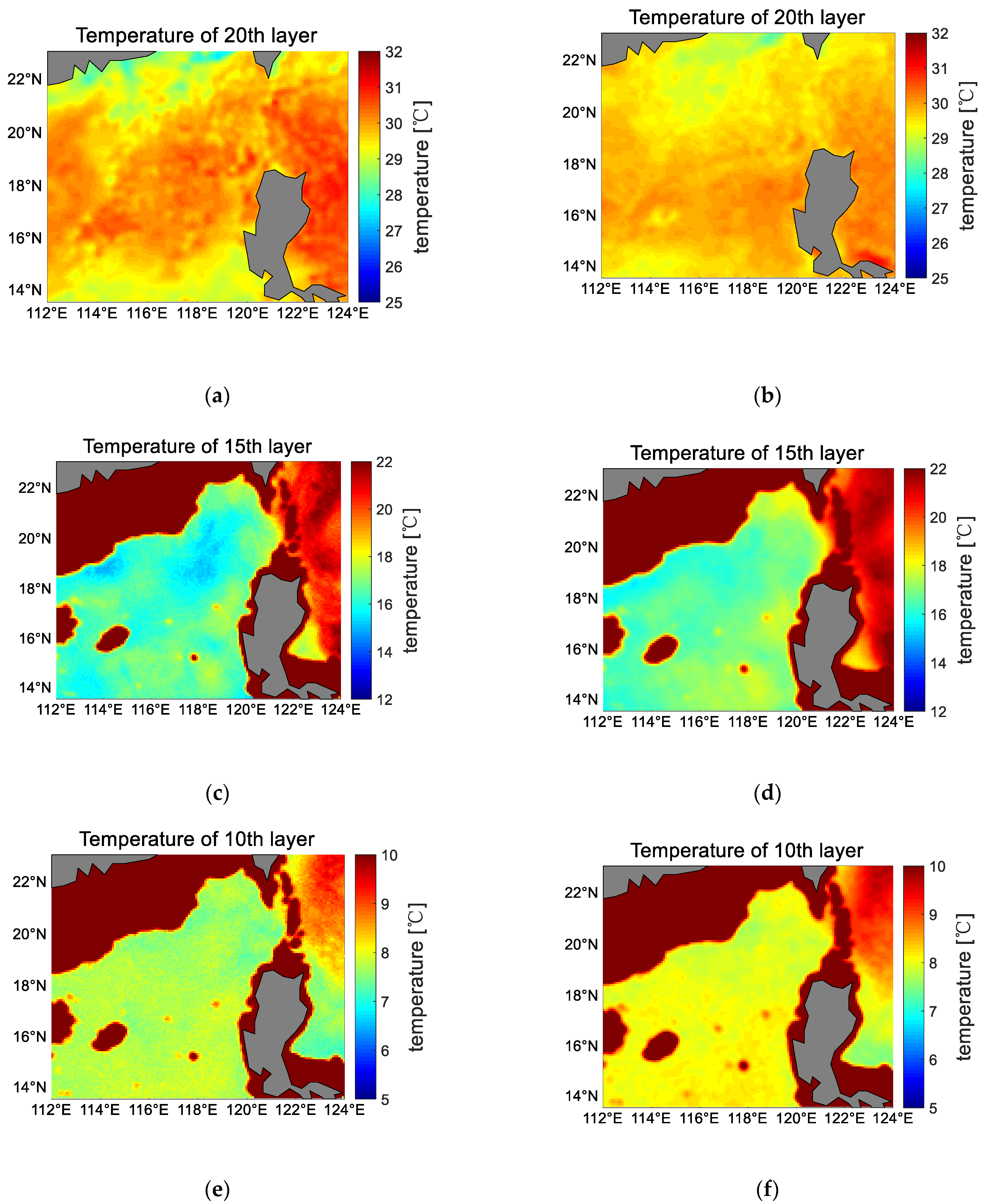
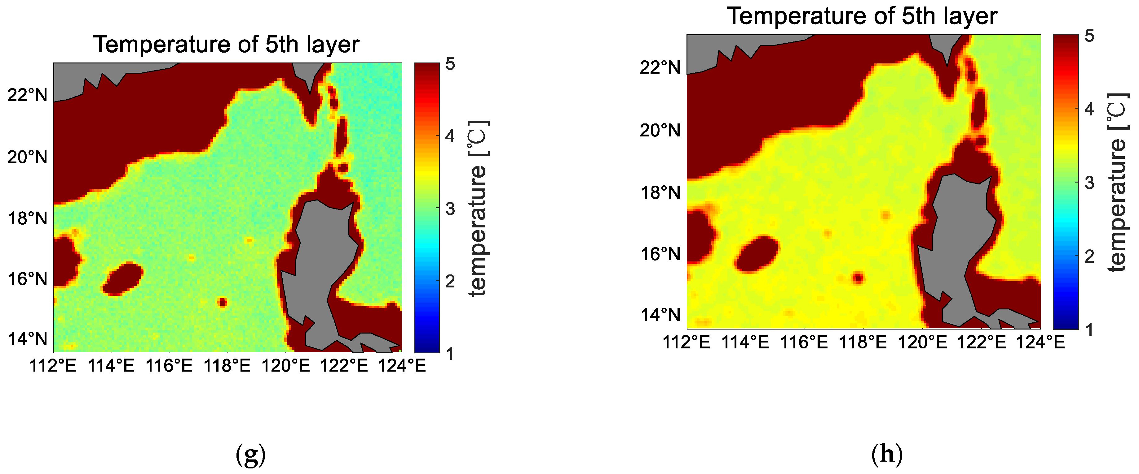
Figure 5 shows the results of the inversion and correction. With the help of DNNs, which is a powerful tool, it is possible to achieve obvious correcting effect with a small amount of vertical information data.
Then, we used a series of Argo observations at different times to evaluate the prediction results through statistics. The evaluation criteria used for following analysis are reported in
Table 1:
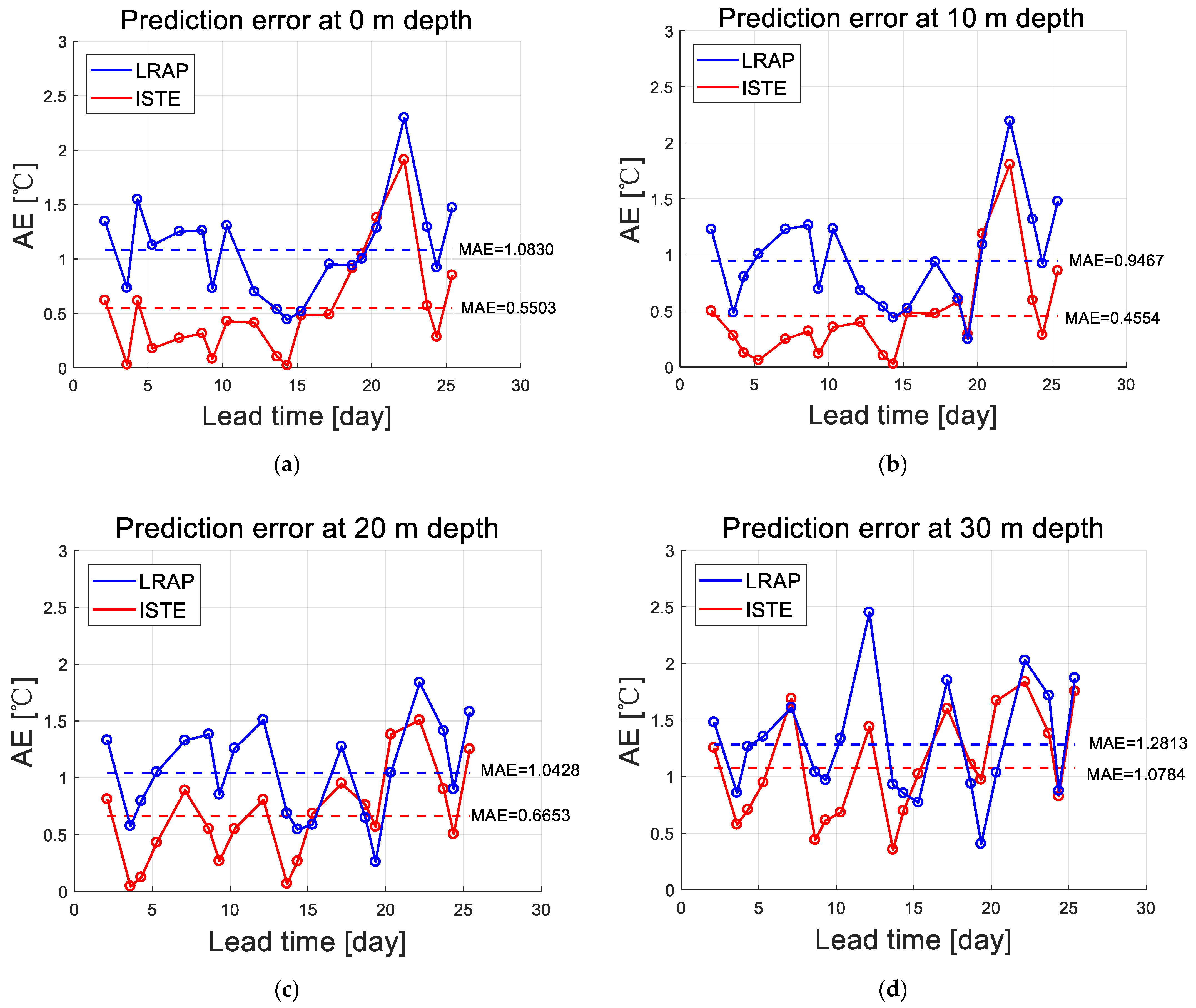
3.1. Mixed Layer
Figure 6 is the prediction errors for mixed layer. We use 0 m, 10 m, 20 m, and 30 m depths to present the prediction errors for mixed layer. The results show that the ISTE method shows a clear superiority over the LRAP method. Compared with the LRAP method, the largest improvement of prediction accuracy in ISTE is at 10 m depth with 52% reduction in error. Additionally, the smallest improvement of prediction accuracy in ISTE is at 30 m depth with 16% reduction in error.
For ISTE, the mean prediction error at 10 m depth is the smallest with the MAE of 0.4554 °C, whereas the mean prediction error at 30 m depth is the largest with the MAE of 1.0784 °C. This is probably because the fluctuations are smallest at 10 m, making it easier for the DNN to capture the pattern hidden in historical data. For 30 m depth, it is closer to the thermocline, which is more volatile and less regular. This results in DNNs not being able to capture data patterns well.
It is also understandable that the error for the sea surface is not the smallest. The sea surface is more influenced by the atmosphere and has more disturbances than the 10 m depth. Therefore, the prediction error at the sea surface is not the smallest.
We also notice that the prediction error is relatively stable in the first 15 days near the sea surface, with an error of around 0.5 °C, whereas there is a significant increase in prediction error after 15 days. As the ISTE algorithm itself does not have the problem of error accumulation over time, this abrupt increase may be due to changes in the background field outside the predicted region. Compared with numerical models, ISTE lacks the information on external changes given by the boundary field. This may lead to a sharp increase in prediction error when there is a dramatic change in the ocean–atmospheric environment outside the region.
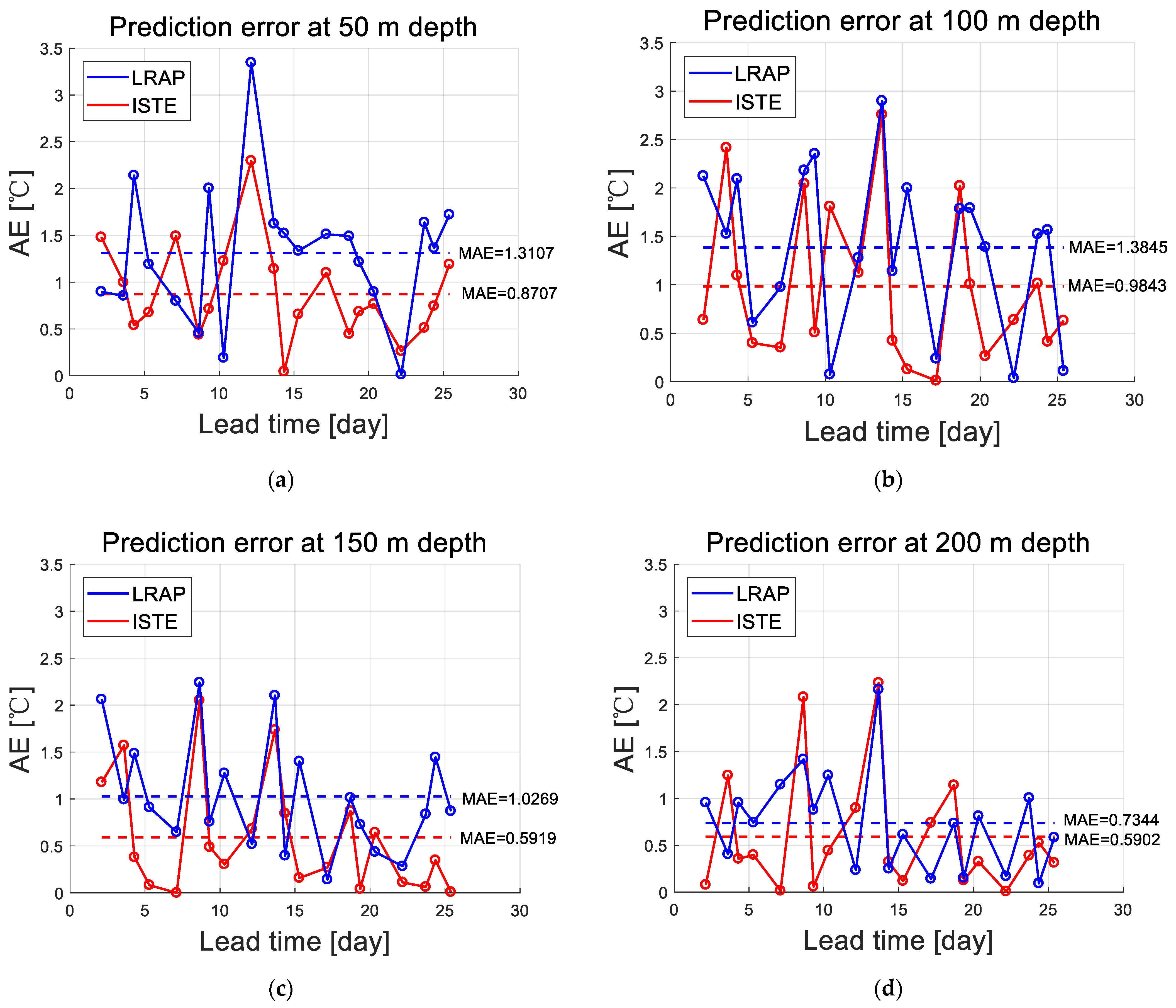
3.2. Thermocline
Figure 7 shows the prediction error for the thermocline. The mean prediction error of ISTE is generally below 1 °C, but there are several extreme errors that greater than 2 °C. This demonstrates that the predictions for the thermocline are more unstable compared with the mixed layer.
The prediction error was greatest at 100 m depth, with an MAE of 0.9843 °C. The prediction error was least at 200 m depth, with an MAE of 0.5902 °C. However, the improvement of ISTE is the smallest at 200 m depth relative to LRAP, where the mean prediction error is reduced by only 20%.
Comparing the predictions of ISTE and LRAP, it can be found that the improvement brought by ISTE is not as visually obvious as the mixed layer and the reduction in mean prediction error is relatively small. This is mainly due to two reasons. The first reason is that the underwater inversion accuracy for SST from satellite remote sensing inevitably decreases when the depth reaches below 50 m, which leads to increasing errors in subsequent prediction. The second reason is that due to the large fluctuations of the thermocline itself. Neither regression nor DNN methods can fully fit the variation pattern. However, even so, the DNN method outperform regression method in terms of mining temperature variation patterns and reducing prediction errors.
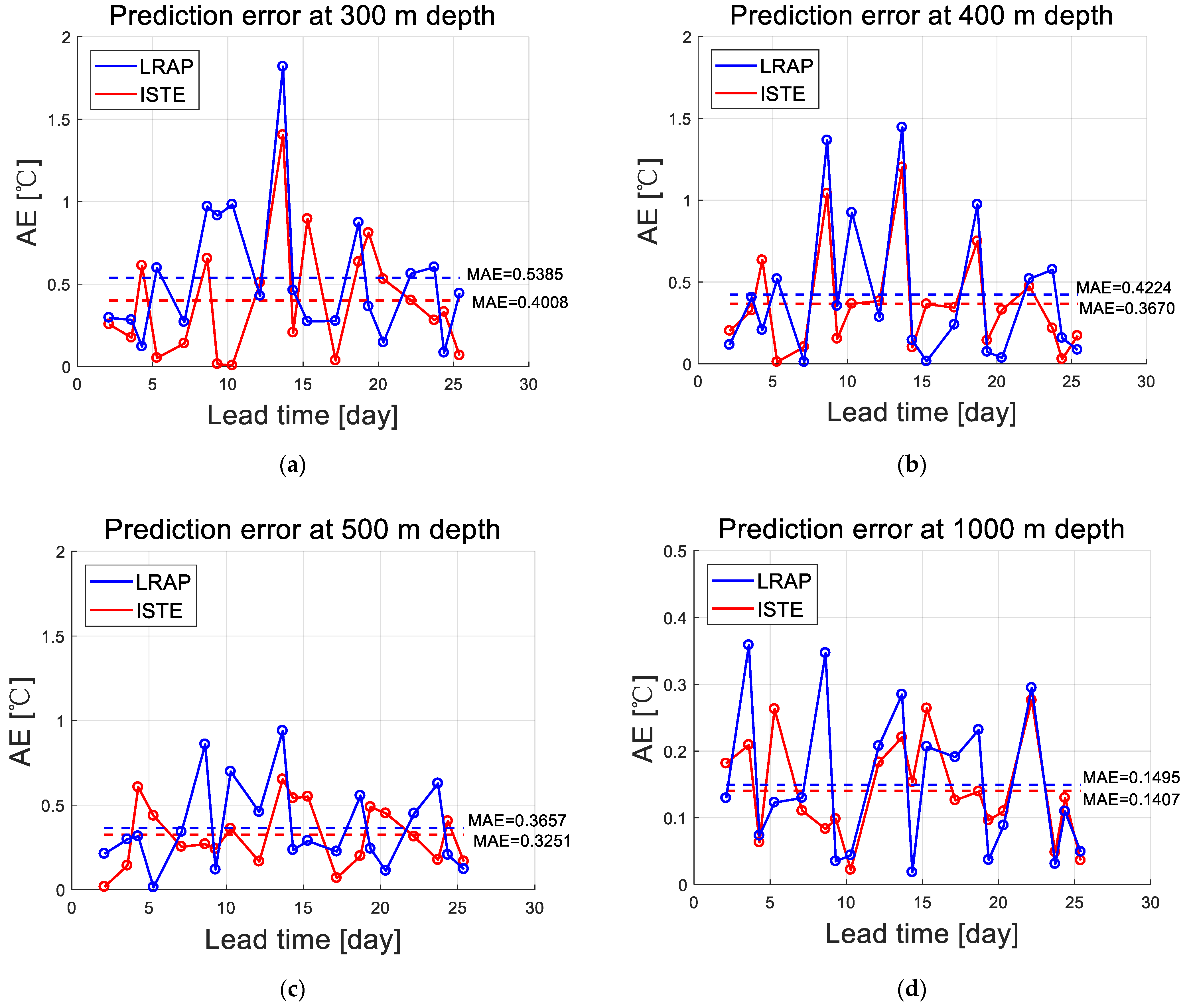
3.3. Deep Layer
Figure 8 shows the prediction errors at the deep layer. The mean prediction error of ISTE remains largely within 0.4 °C. The results show that ISTE still plays a relatively stable role at the deep layer. At the depths of 300, 400, 500, and 1000 m, the prediction errors are smaller than those of LRAP. The results demonstrate that ISTE outperforms LRAP in general. We can also see that as depth increases, ISTE brings very limited improvement at deep layer. This is due to a number of reasons. The temperature fluctuation at deep layer is smaller and therefore the prediction errors are smaller in magnitude. In addition, the reanalysis data used for training does not guarantee high accuracy at deep layer. All these reasons lead to a poorer performance of ISTE at deep layer than in the mixed layer and thermocline.
Although the prediction performance of ISTE at the deeper layers has been reduced, this does not largely affect the value of ISTE applications. It is mainly the mixed layer and thermocline that have a significant impact on human activities at sea, such as sonar detection, offshore fishing, and so on. The improved prediction performance of ISTE for the mixed layer and thermocline will help humans to have a better understanding of the underwater information.
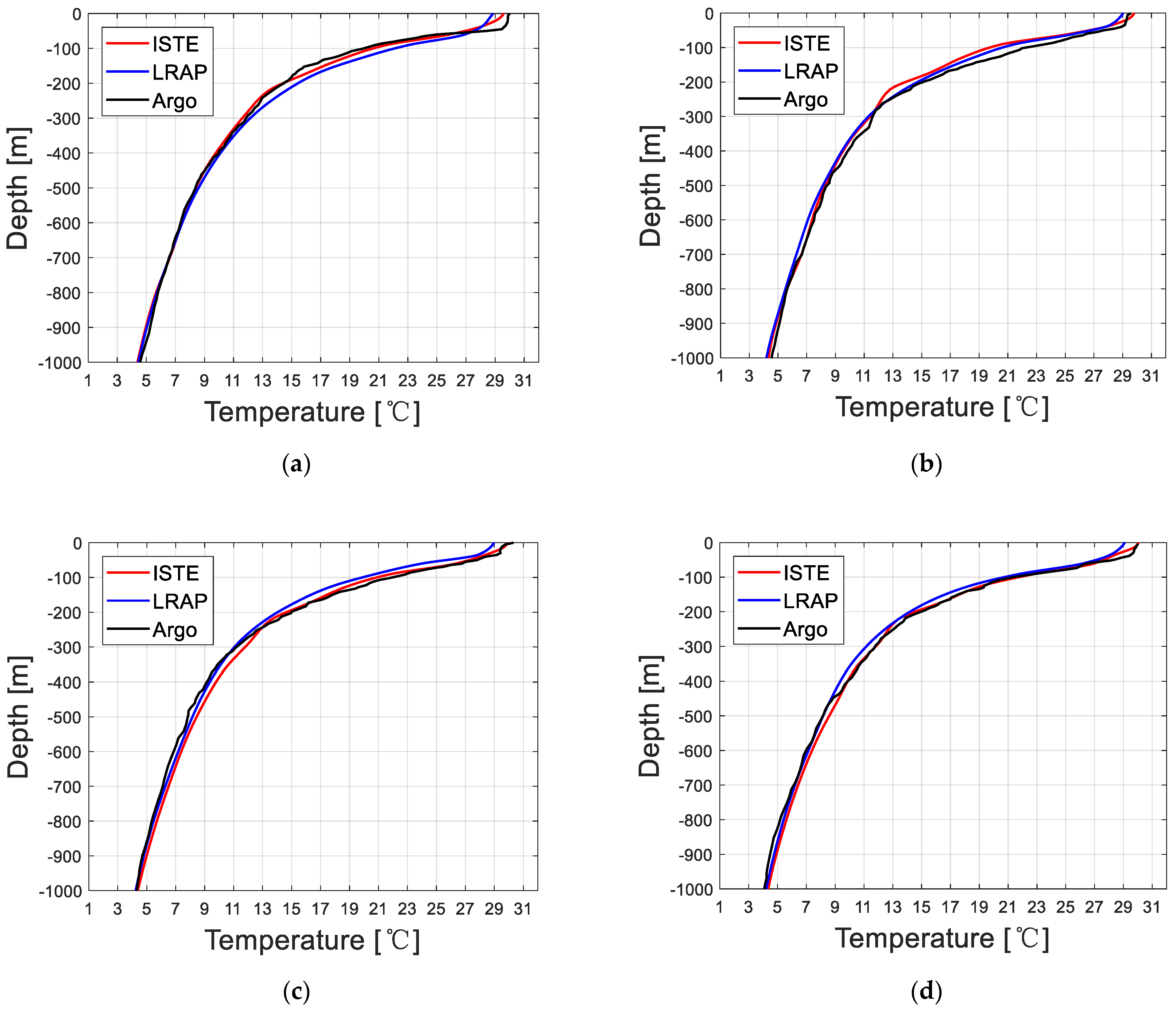
3.4. Vertical Profiles
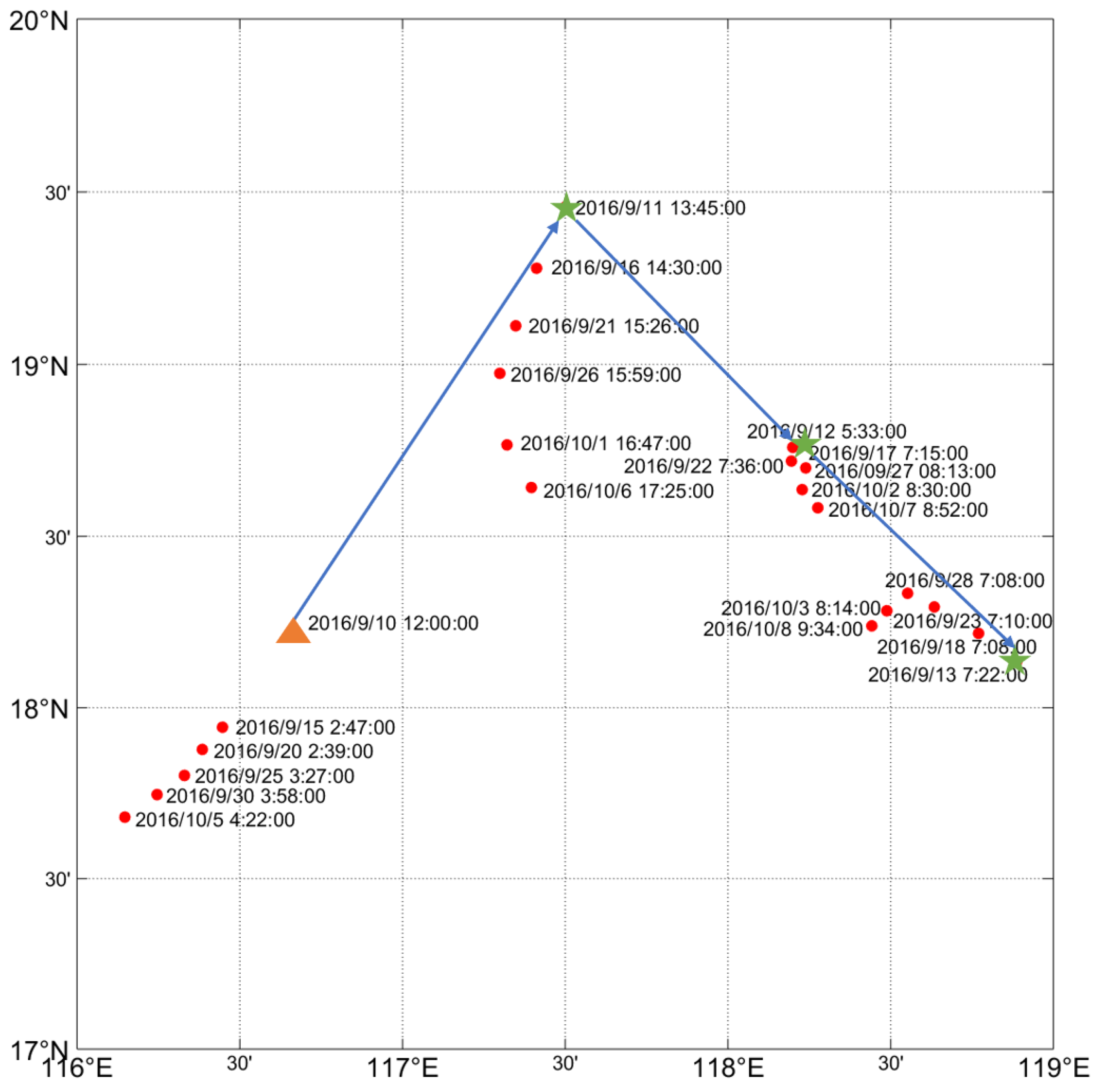
In order to detect the prediction effect in vertical structure, we compare the prediction results with the Argo observation data. In fact, the Argo observations we use are from four Argo buoys, which produce observations every five days. Therefore, we divided the observations into 5 groups to test the prediction effect, as shown in
Figure 9,
Figure 10,
Figure 11,
Figure 12 and
Figure 13. Here, we only present the prediction results for water depths less than 1000 m. The Argo profiles are plotted from all Argo data, the LRAP and ISTE profiles are plotted based on interpolation of the grid data.
The time of group 1 is within 15 September–18 September. In this early stage, ISTE generally match the vertical structure of Argo temperature profiles. In terms of comparing the prediction errors at different depths, the deep layer errors are much smaller than the mixed layer and thermocline.
Figure 9a,c,d show that the ISTE temperature profiles are closer to the Argo temperature profiles compared with LRAP.
The time of group 2 is within 20 September–23 September. In this stage, the SST prediction by ISTE is significantly better than that of LRAP, just like
Figure 9. This proves that we have used the observations effectively.
Figure 10b shows that both ISTE and LRAP present large errors at the thermocline. The maximum error is even more than 2 °C. This may be due to the emergence of temperature changes in this region that are significantly different from its climatic state.
The time of group 3 is within 25 September–28 September.
Figure 11b still shows obvious prediction errors at the thermocline. Meanwhile, the prediction errors of SST are smaller. This also proves that the thermocline temperature is much more difficult to predict than SST. It exhibits more instability.
The time of group 4 is within 30 September–3 October. We notice a significant increase in the prediction error of the ISTE for the SST. This is because the sea surface is more sensitive to the atmospheric environment as time progresses. The accumulated influence of external factors thus leads to a weakening of the correlation between the initial field and the temperature field to be predicted, which in turn increases the prediction error.
The time of group 5 is within 5 October–8 October. We can see that the prediction effect of ISTE generally keep its stability. Additionally, the overall prediction errors of ISTE are smaller than those of LRAP.
Figure 9,
Figure 10,
Figure 11,
Figure 12 and
Figure 13 show that ISTE predicts the structure of the vertical temperature profile in the experimental area well. This demonstrates that ISTE can predict the temperature over the full water depth.
3.5. Statistical Analysis
The above results are the result of training using a 10-year sample of data. In addition to this, sensitivity tests were conducted using 5 and 8 years of sample data, respectively. All the statistical analysis results are shown in
Table 2.
The results show that the ISTE method has a much smaller prediction error. In terms of training results for the 10-year sample, the MAE of ISTE is 0.4949 °C. Compared with LRAP, the MAE of ISTE is reduced by 0.14 °C, whereas the MAPE of ISTE is reduced by 0.6%. ISTE exhibited a lower RMSE of 0.7199 °C, with a 0.21 °C reduction relative to LRAP. ISTE also exhibited a higher R2 of 0.9936, with an improvement of 0.0042 relative to LRAP.
From the results we can also see that the sample length did not have a significant effect on the prediction results, which indicates that the prediction results are not sensitive to the sample length. However, in terms of the characteristics of DNNs, we should use as many sample data as possible to ensure the stability of the data training.
The above experimental results fully demonstrate the effectiveness of the ISTE algorithm, which is significantly better than the traditional LRAP algorithm for the prediction accuracy of ocean temperature.
4. Discussion
Ocean dataset is different from the dataset in other fields such as image and finance. Ocean dataset has its own inherent physical patterns. In terms of ocean temperature, the hidden patterns in temperature data are theoretical vertical modes [
27,
28] or empirical modes [
29] in oceanography. The variation of thermocline or currents are all correlated with the ocean vertical structure changes. It is the correlation between different depth layers that justifies the use of sea surface information to predict the subsurface information [
30,
31]. Thus, AI methods are used to learn these hidden patterns in historical sample data through DNNs and to provide rapid prediction for humans.
In the process of ISE, traditional empirical analysis methods cannot make full use of all SST grid points simultaneously to produce the target inversion field. Besides this, traditional empirical analysis methods can only analyze linear relationships between the SST and subsurface temperature [
8], whereas the AI method are different from the traditional empirical analysis method and have excellent performance that traditional empirical analysis methods do not have.
The driving factor of AI method is the entire SST field, which is a nonlinear correlation with the subsurface temperature field. DNNs can better reflect the spatial correlation characteristics between each grid point of temperature field and capture more structural characteristics of temperature field. Thus, DNN-based ISE can produce a better reconstruction result of temperature field.
In the IC process, the fusion of ship survey observations is superior to traditional linear interpolation. The IC algorithm can largely compensate for missing effective information using the patterns that are mined from historical data. Therefore, the IC process can make full use of the limited ship survey observations to correct the initial estimation field, and thus produce an initial correction field.
For ITE, the DNN-based algorithm can approximate the dynamical equations to some extent. It can fit the patten of historical data and achieve an approximate prediction. This algorithm establishes a one-to-one mapping relationship between the moment to be predicted and the initial field. The advantage of this algorithm is that there is no error accumulation over time. The stability of the prediction error can be guaranteed.
Through experiments, it can be found that the sea thermocline temperature (STT) is more difficult to be predicted compared with SST. The reason is that the ocean is different from a general data set. The real ocean is a 3D fluid affected by gravity, which forms a layered structure due to the difference in density, as shown in
Figure 9,
Figure 10,
Figure 11,
Figure 12 and
Figure 13. When the ocean is affected by external forces, it will cause sharp fluctuations in the thermocline. The SST change is relatively stable compared with STT and the SST changing regulations is easier to be captured by DNNs, which can lead to better prediction effects. Therefore, since the thermocline has stronger volatility and uncertainty, the STT changing regulations with time is more difficult to be captured compared with SST.
Taken together, the ISTE algorithm can makes full use of satellite remote sensing observations and limited ship survey observation data. Then, achieve the spatial and temporal extension of available information. In fact, this process achieves 4D temperature prediction. Therefore, the ISTE algorithm can be as an effective shipborne prediction method. The prediction performance of ISTE is significantly better than the traditional LRAP methods.
In this article, only an experimental study of the ISTE algorithm for temperature prediction has been carried out. In practice, we can obtain more types of observational data, including sea surface height (SSH) and sea surface salinity (SSS). Based on these facts, we will consider these factors in the next step.
- (1)
Develop ISE algorithms that can fuse all satellite remote sensing data, including SST, SSH and SSS.
- (2)
Develop IC algorithms with temperature and salt constraints.
- (3)
Develop multi-factor coupled ITE prediction algorithms.
- (4)
Consider exploring more advanced DNN structures that combine multiple neural networks.
We expect that these works will further improve the prediction accuracy for ocean environment. The more advanced technology will enable the ISTE algorithm to be used in a wider application context, including weather prediction and climate prediction.
5. Conclusions
Satellite remote sensing data can provide data with high temporal and spatial resolution, but they are limited to the surface and cannot provide underwater information. For shipborne prediction, it is convenient to obtain ship survey observations to access accurate vertical information. The ISTE algorithm can be used to fully integrate the satellite remote sensing data and ship survey observation data to achieve a 4D ocean environment prediction.
This paper demonstrates the effectiveness of the ISTE algorithm through prediction experiments on ocean temperatures. The experimental results show that the MAE of ISTE is around 0.5 °C, the MAPE is around 4%, the RMSE is around 0.7 °C and the R2 is 0.9936, Relative to the observations. Compared with the traditional LRAP method, the prediction accuracy of ISTE has been significantly improved.
The ISTE algorithm is a convenient, practical, and effective method for shipborne prediction. We anticipate that the DNN-based ISTE algorithm will help humans to obtain timely information about the ocean environment and further benefit relevant marine operations, including but not limited to sonar detection and offshore fishing.


