Article

Hyperspectral Image Denoising via Adversarial Learning

1
Key Laboratory of Specialty Fiber Optics and Optical Access Networks, Joint International Research Laboratory of Specialty Fiber Optics and Advanced Communication, Shanghai Institute of Advanced Communication and Data Science, Shanghai University, Shanghai 200444, China
2
Hangzhou Institute for Advanced Study, University of Chinese Academy of Sciences, Hangzhou 310024, China
*
Author to whom correspondence should be addressed.
Remote Sens. 2022, 14(8), 1790; https://doi.org/10.3390/rs14081790
Submission received: 25 February 2022 / Revised: 30 March 2022 / Accepted: 3 April 2022 / Published: 7 April 2022
(This article belongs to the Special Issue Remote Sensing Image Denoising, Restoration and Reconstruction)

Abstract

:
Due to sensor instability and atmospheric interference, hyperspectral images (HSIs) often suffer from different kinds of noise which degrade the performance of downstream tasks. Therefore, HSI denoising has become an essential part of HSI preprocessing. Traditional methods tend to tackle one specific type of noise and remove it iteratively, resulting in drawbacks including inefficiency when dealing with mixed noise. Most recently, deep neural network-based models, especially generative adversarial networks, have demonstrated promising performance in generic image denoising. However, in contrast to generic RGB images, HSIs often possess abundant spectral information; thus, it is non-trivial to design a denoising network to effectively explore both spatial and spectral characteristics simultaneously. To address the above issues, in this paper, we propose an end-to-end HSI denoising model via adversarial learning. More specifically, to capture the subtle noise distribution from both spatial and spectral dimensions, we designed a Residual Spatial-Spectral Module (RSSM) and embed it in an UNet-like structure as the generator to obtain clean images. To distinguish the real image from the generated one, we designed a discriminator based on the Multiscale Feature Fusion Module (MFFM) to further improve the quality of the denoising results. The generator was trained with joint loss functions, including reconstruction loss, structural loss and adversarial loss. Moreover, considering the lack of publicly available training data for the HSI denoising task, we collected an additional benchmark dataset denoted as the Shandong Feicheng Denoising (SFD) dataset. We evaluated five types of mixed noise across several datasets in comparative experiments, and comprehensive experimental results on both simulated and real data demonstrate that the proposed model achieves competitive results against state-of-the-art methods. For ablation studies, we investigated the structure of the generator as well as the training process with joint losses and different amounts of training data, further validating the rationality and effectiveness of the proposed method.

Graphical Abstract

1. Introduction

Hyperspectral sensors collect spatial and spectral information from the Earth’s surface, producing hyperspectral images (HSIs) with massive discrete wavebands. Compared to general RGB images, HSIs often contain abundant spectral information, the exploration of which is critical for various remote sensing applications [1] such as classification [2,3], unmixing [4] and tracking [5]. However, due to sensor instability and atmospheric interference, HSIs often suffer from various kinds of noise [6] such as Gaussian noise, impulse noise, stripe noise and deadlines. Gaussian noise represents statistical noise with a normal distribution. The impulse noise is the white or black pixel that occurs randomly, due to the circuit failure, power switching, etc. The stripe noise is the one with striped distributions which are often caused by instrument instability and light interference. Furthermore, deadlines can be regarded as a special case of stripe noise. Kinds of noise reduce the quality of HSIs, which easily degrades the performance of downstream HSI tasks.
To overcome the above issue, various methods have been proposed for HSI denoising from different perspectives. Early works considered HSI denoising as the extension of gray or RGB image denoising. They often utilize the existing denoising methods band-wisely to remove noise in HSIs, e.g., block-matching, 3D filtering (BM3D) [7] and weighted nuclear norm minimization (WNNM) [8]. However, only the spatial information is considered in these works, while the rich spectral information is neglected, resulting in spectral distortion in the outputs.
To model the correlation in the spectral dimension, researchers have proposed spatial-spectral-based methods which jointly utilize spatial and spectral information to reduce the HSI noise. Othman et al. [9] proposed a hybrid spatial-spectral noise removal (HSSNR) method working with wavelet shrinkage, which benefits from both the spatial and spectral information. A denoising framework with bivariate wavelet thresholding and principal component analysis was proposed by Chen et al. [10] to reduce the dimensionality of HSIs and simultaneously remove the noise. Considering the noise intensity difference in different bands, Yuan et al. [11] proposed a spectral-spatial adaptive total variation (TV) model. As the extension of the BM3D algorithm, Maggioni et al. [12] presented the BM4D algorithm with the grouping and collaborative filtering paradigm for the 3D cube data noise reduction. He et al. [13] proposed the removal of mixed noise via the TV-regularized low-rank matrix factorization.
Since an HSI can be viewed as a collection of multiple 2D images, tensor-based denoising methods have been proposed by treating the HSI as a 3D tensor. Liu et al. [14] presented the parallel factor analysis (PARAFAC) method to estimate the clean HSIs with a powerful multilinear algebra model. By explicitly considering the spatial nonlocal similarity and the correlation among bands of multispectral images, Peng et al. [15] constructed the decomposable nonlocal tensor dictionary learning model for denoising. Wang et al. [16] proposed the low-rank tensor decomposition with the anisotropic spatial-spectral TV (LRTDTV) method by identifying the structures of noise-free images and the noise for the HSI denoising task. Fan et al. [17] proposed the spatial-spectral TV regularized low-rank tensor factorization (SSTV-LRTF) method which can maintain the spatial smoothness while removing the Gaussian noise. Though existing methods have obtained decent performance in certain cases, there are still several bottlenecks that need to be addressed. First of all, these methods manage to achieve better results in relatively simple cases and are unable to satisfy the complex mixed noise. Secondly, HSI denoising tasks are generally regarded as an optimization problem to be solved iteratively in traditional algorithms, bringing time-consuming drawbacks. Therefore, it is necessary to find an efficient and robust method to address the aforementioned issues.
In recent years, deep learning-based methods have been successfully applied in the image processing field due to the better capability of the graphics processing unit (GPU) with advanced results in various vision tasks such as classification, detection and image synthesis. Most recently, some researchers have applied deep neural network-based methods in HSI denoising tasks. Xie et al. [18] employed a deep stage convolutional neural network (CNN) with trainable non-linearity functions in an HSI denoising task for the first time and confirmed its reliability. Yuan et al. [19] proposed a spatial-spectral convolutional neural network named HSID-CNN to learn a non-linear mapping between the noisy and noise-free images, simultaneously considering the spatial and spectral information. Inspired by the structure of UNet [20], Dong et al. [21] proposed a modified 3D UNet to fully exploit the multiscale information of HSIs and decompose 3D convolutional kernels to reduce the computational complexity. Zhang et al. [22] presented a spatial-spectral gradient network (SSGN), which simultaneously handles different types of noise.
Apart from optimizing the generated predictions towards given objectives, the generative adversarial network (GAN) [23] consists of a generator and a discriminator trained in an adversarial fashion. The generator learns from the distribution of real data to generate the synthetic data, and the discriminator tries to distinguish the output of the generator from the real data [24]. With the joint training, the generator and discriminator finally reach the Nash Equilibrium. GAN has been widely utilized in image synthesis-related tasks such as super-resolution [25], face synthesis [26] and image restoration [27]. Jelmer et al. [28] trained a CNN jointly with a discriminator in a medical images-denoising task to improve the CNN ability to generate noise-free medical images. Chen et al. [29] proposed a GAN-based network to reduce the speckle noise and preserve the texture details in the optical coherence tomography images. Lyu et al. [30] proposed a novel denoising GAN-based model to remove the mixed noise in RGB images and the generator learns the direct mapping from the noisy images to clean ones. To solve the blurriness issue caused by current CNNs, Niu et al. [31] applied the GAN-based network in the cell image denoising task which can recover feature details in the cell images.
In contrast with general RGB images, the abundant spectral information of HSIs needs to be leveraged during the denoising process. Inspired by the architecture of GANs, we proposed an adversarial learning-based residual network for handling the complex cases of mixed-noise removal including Gaussian noise, impulse noise, stripe noise, deadlines and their mixture. The main contributions of our proposed model can be summarized as follows:
  • We designed an adversarial learning-based network architecture to model the difference between noisy and noise-free HSIs. The adversarial learning mechanism encourages the network to generate more realistic clean HSIs.
  • For the generator, we designed a Residual Spatial-Spectral Module (RSSM) with an UNet-like structure to capture the subtle noise distribution of each HSI by fully exploring both spatial and spectral features at multiple stages. The generator is trained with joint loss functions including the reconstruction loss to recover the details of images, the structural loss to maintain the structural similarity and the adversarial loss to improve the realistic degree of the generated images. For the discriminator, to distinguish between the generated and ground-truth clean data, we propose a Multiscale Feature Fusion Module (MFFM) to enhance the discrimination ability by leveraging the features across scales.
  • Due to the lack of training data for the HSI denoising task, we collected an additional dataset named Shandong Feicheng dataset. Comprehensive experiments were conducted on public and collected datasets, and the experimental results demonstrate that the proposed model achieves results rivalling those of state-of-the-art methods.
The remainder of this paper is organized as follows. Section 2 introduces the proposed network in detail. Section 3 presents the investigated datasets and reports the experimental results including comparisons with state-of-the-arts denoising methods, comprehensive ablation results, and real-data experiments. Finally, Section 4 concludes the proposed method of our work.

2. Materials and Methods

2.1. HSIs Degradation

Generally, an HSI can be denoted by a 3D tensor Y R H × W × C and can be described as
Y = X + N ,
where X R H × W × C is the noise-free HSI data, N R H × W × C is the noise of HSI data including Gaussian noise, impulse noise, stripe noise and deadlines, H and W are the height and width of the HSI, respectively, C represents the number of spectral bands. Naturally, the HSI denoising task is to estimate the noise-free HSI data X from the noisy HSI data Y.

2.2. Model Overview

Inspired by the advanced image restoration ability of adversarial learning, we designed a GAN-based model for the HSI denoising task. For a general GAN, the generator G learns the distribution of noisy data whilst the discriminator D estimates the probability that the data come from the clean ground truth or the generator. When D cannot judge whether the image is true or fake and G cannot generate a more realistic image to deceive D, the training process reaches stability. Considering the abundant spatial-spectral information of HSIs, appropriate designs for the generator and discriminator are necessary. To improve the network’s estimation of noisy areas and noise intensity, we adopt the residual blocks [32] to each layer of the generator, so that the generator can capture nuanced details while reducing the gradient-vanishing problem. In terms of the discriminator, to make the network fully utilize the spatial-spectral information of HSIs, the multiscale feature extraction mechanism is employed in the discriminator. In part of the loss function, to constrain the training process from diverse perspectives, we jointly consider the pixel-wise difference, structural similarity and adversarial penalty as the combined loss function with appropriate weights. The overall network architecture is shown in Figure 1.

2.3. Generative Network

As shown in Figure 1, the generator is a UNet-based network with a residual learning mechanism. Considering the sparsity of the noise, instead of learning the complex direct mapping from noisy HSIs to their noise-free counterparts, the noise distributions can be relatively easier to capture. More specifically, the generator mainly consists of three parts, including the initial convolutional layer, the UNet-based feature extraction module and the recovering convolutional layer. In the initial convolutional layer, 3 × 3 convolutional kernels are used to acquire the initial feature maps with 64 channels. These feature maps are then fed to the UNet-based feature extraction module, which is composed of an encoder part and a decoder part. To obtain the feature maps of the noise distribution, we downsampled the input three times by maxpooling operation with 2 × 2 kernel size in the encoder part. Accordingly, we upsampled the encoded features three times by deconvolutional operation with a 2 × 2 kernel size to obtain the spatial information of noise.
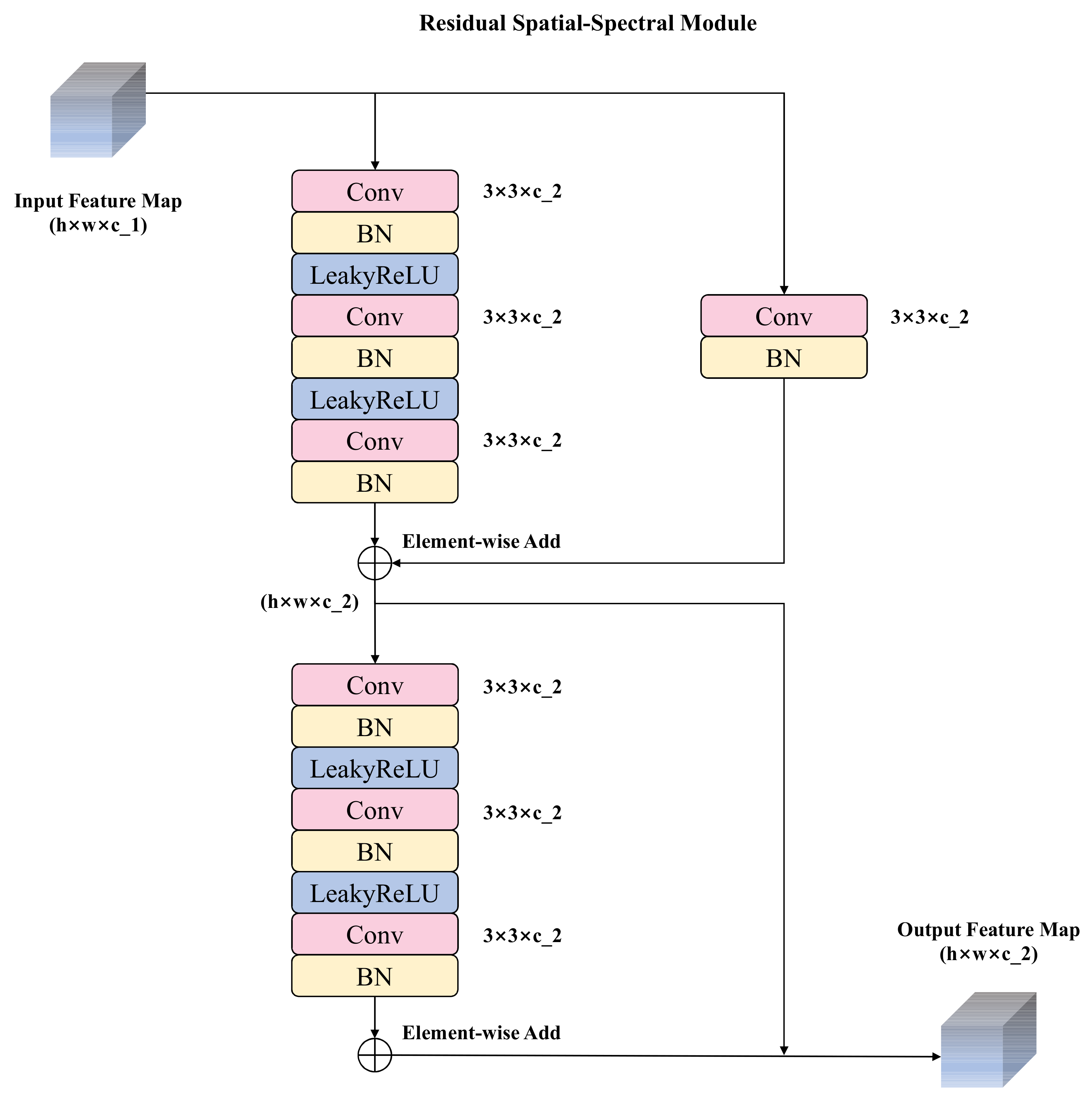
Between the adjacent downsampling layers and upsampling layers, the RSSM are proposed to extract feature maps. As shown in Figure 2, there are two cascaded residual blocks in the RSSM.
The first residual block consists of two branches including three convolutional layers and a shortcut connection with a linear projection in which we expand the number of feature map channels and extract essential spectral features. The second one consists of two branches including three convolutional layers and a shortcut connection, in which higher-level features and larger receptive fields are obtained to enhance the spatial features. It can be described as:
y = C 3 2 ( C 3 1 ( x ) + S ( x ) ) + C 3 1 ( x ) + S ( x ) ,
where x is the input, y is the output of the first residual block, C 3 1 ( · ) , C 3 2 ( · ) denotes the three convolutional layers in the first residual block and the second block, respectively, and S ( · ) indicates the shortcut connection operation with a linear projection. Moreover, 3 × 3 convolutional kernels are utilized in all convolutional layers in RSSM that the spectral information and the neighborhood information can be fully exploited. With the multiple connected convolutional layers in RSSM, the receptive field becomes larger so that the spatial information can also be fully considered simultaneously. Taking advantage of the different levels of the feature maps, we concatenate the same-sized feature maps as skip connections.
It is worth noting that the noise values in the HSIs are not significantly larger than zero; thus, we utilize the LeakyReLU as the activation function in the whole generator. Meanwhile, the LeakyReLU function can also prevent the network from zero gradients. The LeakyReLU function we adopted is defined as:
y = x , x 0 , a x , x < 0 ,
where x is the input, y is the output of the LeakyReLU function and a is a constant parameter in the range of ( 0 , 1 ) , which is empirically set to 0.2 . The last recovering convolutional layer is added to keep the size of the output feature maps the same as the input images, and the output feature maps are finally added to the input images.

2.4. Discriminative Network

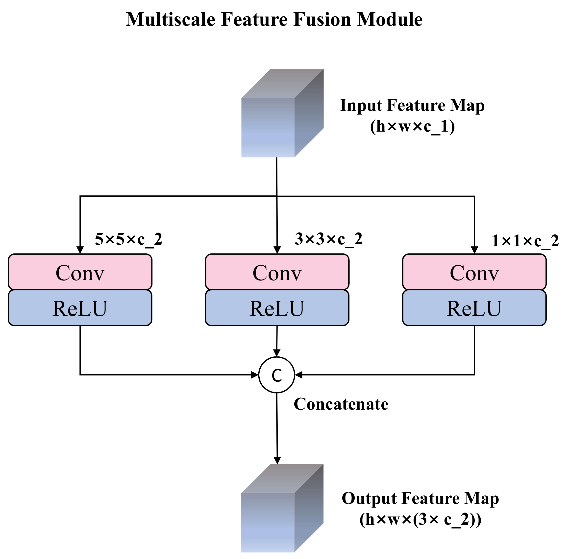
To obtain more realistic denoising results via adversarial learning, we designed a fully convolutional network with MFFM as our discriminator. The MFFM structure is shown in Figure 3.
Taking both spatial and spectral information into consideration, we utilized two multiscale feature extraction blocks with three different convolutional kernel sizes. To exploit the correlation in the spectral dimension, 1 × 1 convolutional kernels are utilized to extract the spectral feature of each pixel. For leveraging the spatial information, 3 × 3 convolutional kernels focus on the neighboring features around the center pixel, and 5 × 5 convolutional kernels can obtain more abundant spatial features with large receptive fields. The multiscale feature maps are then aggregated to generate representative features. Instead of element-wisely addition, we employed the concatenation operation of multiscale feature maps on the channel dimension to preserve more detailed information. The MFFM is defined as:
y = C a t [ R e L u ( C 1 ( x ) ) , R e L U ( C 3 ( x ) ) , R e L U ( C 5 ( x ) ) ] ,
where x is the input feature map, y is the output of the MFFM, C a t [ · ] represents the concatenation operation, R e L u ( · ) denotes the ReLu activation function and C n ( · ) represents the convolutional layer with an n × n kernel size. To obtain more accurate local details, we designed a 32 × 32 matrix instead of one value as the final output of the discriminator inspired by PatchGAN [33]. Each spatial element of output represents a 16 × 16 receptive field in the input data and the value measures whether the given region from the input data is true.

2.5. Loss Function

To ensure the network generates realistic hyperspectral images, three types of loss functions were jointly considered, including reconstruction loss structural loss and adversarial loss. The reconstruction loss was utilized to measure the distance between the generated HSIs and ground truth. The structural loss captures the structural differences between the generated HSIs and ground truth, while the adversarial loss measures the authenticity of generated HSIs, which improves the image quality.
We utilized the Mean Square Error (MSE) as the reconstruction loss function to reduce the difference between the generated HSIs and noise-free ones:
L r = ( X G ( Y ) ) 2 ,
where G ( · ) means the generator, X is the noise-free HSIs and Y is the input HSIs. Reconstruction loss is the most commonly used loss function for general image reconstruction. However, the reconstruction loss often produces blurry results indicating that only utilizing the reconstruction loss is not enough.
For structural loss, we employed the structural similarity (SSIM) to reduce the structural differences between the generated HSIs and noise-free ground-truth. Details of the SSIM index can be found in [34]. The value of the SSIM index ranges from 0 to 1, and the larger SSIM index means a more similar structure between the two images. Therefore, L s is defined as:
L s = 1 S S I M ( X , Y ) ,
where S S I M ( X , Y ) indicates the similarity between X and Y.
As for the adversarial loss, the objective of a general GAN can be expressed as
m i n G m a x D E x P d a t a ( x ) [ l o g D ( X ) ] + E x P G ( x ) [ l o g ( 1 D ( G ( X ) ) ) ] ,
where D ( · ) represents the discriminator. For the discriminator, we maximize the objective function to identify the real data or the false data. For the generator, we minimize the objective function so that the generator can fool the discriminator. We train G ( · ) and D ( · ) simultaneously to make the generated image close to the real data. Therefore, the adversarial loss in our case can be described as:
L a = m a x D E x P d a t a ( x ) [ l o g D ( X ) + l o g ( 1 D ( G ( X ) ) ) ] .
In summary, we define the joint loss function as:
L = λ r L r + λ s L s + λ a L a .
where λ r , λ s and λ a represent the weights of the reconstruction loss, the structural loss and the adversarial loss, respectively.

2.6. Implementation Details

In the network training process, we utilized Adam [35] to optimize the proposed network with momentum parameters of 0.9 and 0.99, while the initial learning rate was set to 0.001. We employed the stage-wise training strategy, i.e., training the generator and the discriminator separately first, and then the generator and the discriminator were trained jointly to further finetune the performance of the generated HSIs. The batch size and the maximum number of epochs were set to 16 and 300, respectively. It is worth noting that the weights of the reconstruction loss, the structural loss and the adversarial loss were empirically set to 100, 1, 0.001, respectively. The training process of the proposed network takes approximately 30 h on the Ubuntu 18.04 operating system with a GTX 3090 GPU. Under the same setting, the proposed model can process approximately 672 HSIs with the size of 128 × 128 × 63 per second for inference.

3. Results and Discussion

3.1. Datasets

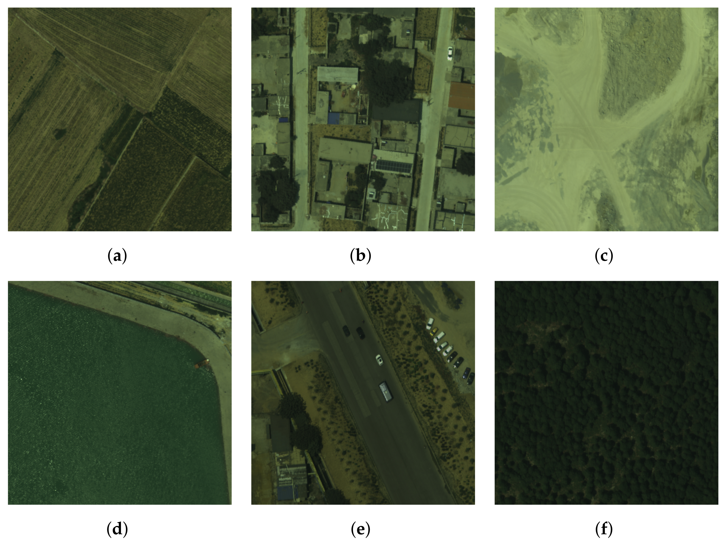
The evaluation of denoising models was conducted on both public and collected datasets for training and testing. Currently available HSI datasets are mostly used to evaluate hyperspectral classification and unmixing tasks. Given the lack of abundant hyperspectral dataset for the denoising task, we collected a relatively large-scale hyperspectral dataset in Feicheng City, Shandong Province, China. The Feicheng Hyperspectral Dataset was obtained by China’s new generation of airborne high-resolution imaging spectrometer (high score special aviation hyperspectral spectrometer). The wavelength range is from 0.4 to 1 μ m, containing 63 wavebands, and the spatial resolution is 12.5 cm per pixel. The size of the whole hyperspectral image is 262,748 × 10,983. To obtain a dataset with diverse scenes, we chose six of them and cropped them to the size of 128 × 128 , resulting in a denoising dataset containing 1596 HSIs, named Shandong Feicheng Denoising (SFD) dataset. As shown in Figure 4, the six scenes are farmland, building, dirt, lake, road and tree. Each scene apart from the road of the SFD dataset consists of three hundred images and the road scene consists of 96 HSIs.
Apart from the collected dataset, five public HSI datasets were employed in this paper, including the Washington DC Mall, Pavia University, Xiongan New Area [36], Indian Pines, Urban and EO-1 Hyperion datasets; the details of these datasets are described as follows:
  • Washington DC Mall dataset was obtained by the Hyperspectral Digital Imagery Collection Experiment (HYDICE) airborne sensor with a wavelength range of 0.4–2.4 μ m containing 191 wavebands after removing the water absorption bands. The image size is 1208 × 307 with a spatial resolution of 5 m per pixel.
  • Pavia University dataset, a 610 × 610 pixels image, was collected by the Reflective Optics System Imaging Spectrometer (ROSIS), where the wavelength ranges from 0.43 to 0.86 μ m and includes 103 wavebands. The spatial resolution is approximately 1.3 m per pixel.
  • Xiongan New Area dataset was acquired by the visible and near-infrared imaging spectrometer and its spectral range is from 0.4 to 1 μ m with 250 wavebands. The image size is 3750 × 1580 pixels with a spatial resolution of 0.5 m per pixel.
  • Indian Pines dataset was gathered by the AVIRIS sensor in northwestern Indiana consisting of 145 × 145 pixels. The spectral range is from 0.4 to 2.5 μ m with 200 wavebands after removing the water absorption bands. The spatial resolution is 20 m per pixel.
  • Urban dataset was obtained by HYDICE airborne sensor, containing 307 × 307 pixels. The wavelength of the hyperspectral image ranges from 0.4 μ m to 2.5 μ m with 210 wavebands, and the spatial resolution is 2 m per pixel.
  • EO-1 Hyperion dataset covers 166 wavebands after removing the water absorption bands, consisting of 400 × 200 pixels.

3.2. Experimental Setup

By referring to the experimental protocols in [21,22,37,38], to validate the performance of the proposed network for the HSI denoising task, the simulated noisy HSIs and real noisy HSIs were employed. The commonly used public HSIs datasets including Washington DC Mall, Pavia University, Xiongan New Area and the proposed SFD were used for training and testing on simulated cases. Moreover, we utilized the Indian Pines, Urban and EO-1 Hyperion datasets to verify the effectiveness of the proposed network and conduct comparisons against state-of-the-art methods for the real data.
During the simulated HSI denoising process, different types of noise were added to the noise-free images. Similar to [22,37,38], in this paper, we simulated five mixed-noise cases of noise as follows:
  • Case 1 (Gaussian noise): All wavebands were corrupted by Gaussian noise with a signal-to-noise rate (SNR) value of 20 dB.
  • Case 2 (Gaussian + impulse noise): All wavebands were corrupted by Gaussian noise as in Case 1, and 10 wavebands were randomly chosen to add the impulse noise. In our experiments, impulse noise was randomly set to 0 or 1.
  • Case 3 (Gaussian + impulse + stripe noise): All wavebands were corrupted by Gaussian and impulse noise as in Case 2, and 10 wavebands were randomly chosen to add the stripe noise. In each band, stripe noise was randomly added to 20–40 lines.
  • Case 4 (Gaussian + impulse + deadline noise): All wavebands were corrupted by the Gaussian and impulse noise as in Case 2, and 10 wavebands were randomly chosen to add deadlines. In each band, deadlines were randomly added to 0–5 lines.
  • Case 5 (All mixed noise): Four kinds of noise were added to the HSIs. Impulse noise, stripe noise and deadline were added as previously described. All wavebands were corrupted by Gaussian noise with SNR values of 10, 20, 30, 40 dB in Case 5_1, 5_2, 5_3, 5_4, respectively.
The four datasets we used for training and testing were normalized to 0–1 with the min–max normalization method. There are 3597 samples in the training and validation sets, 90% of the data are used for training and 10% for validation and another 1334 samples are utilized for testing. In detail, we trained the proposed network on four datasets simultaneously. Since images from different datasets were acquired with different sensors, the HSIs in four datasets vary with the number of wavebands. During data preprocessing, we selected 63 bands for each dataset to ensure all that HSIs have a similar spectral range. The number 63 was selected since the smallest band size is 63 among all used datasets.

3.3. Comparative Experiment with Simulated Data

In comparative experiments, the proposed network was compared with eight HSIs’ denoising methods including nuclear norm minimization (NNM) [39], block-matching and 4-D filtering (BM4D) [12], weighted nuclear norm minimization (WNNM) [8], low-rank total variation (LRTV) [13], weighted Schatten p-Norm minimization (WSNM) [40], low-rank tensor decomposition total variation (LRTDTV) [16], 3D total variation (3DTV) [37] and fast hyperspectral denoising (FastHyDe) [41]. For fair comparisons, the compared works were implemented by referring to the publicly released code. To measure the performance of our results, three indicators were used: mean peak signal-to-noise ratio (MPSNR), mean structural similarity (MSSIM), mean spectral angle distance (MSAD). MPSNR represents the intensity of the noise in the image. MSSIM indicates the structural similarity of two images. MSAD denotes the spectral difference of each pixel in two images. It should be denoted that the higher MPSNR values represent the lower noise intensity, namely the better performance. Furthermore, the higher MSSIM values indicate that the denoising HSIs are closer to the noise-free HSIs in structure. Lower MSAD values mean a smaller spectral distance between the denoising HSIs and noise-free HSIs.
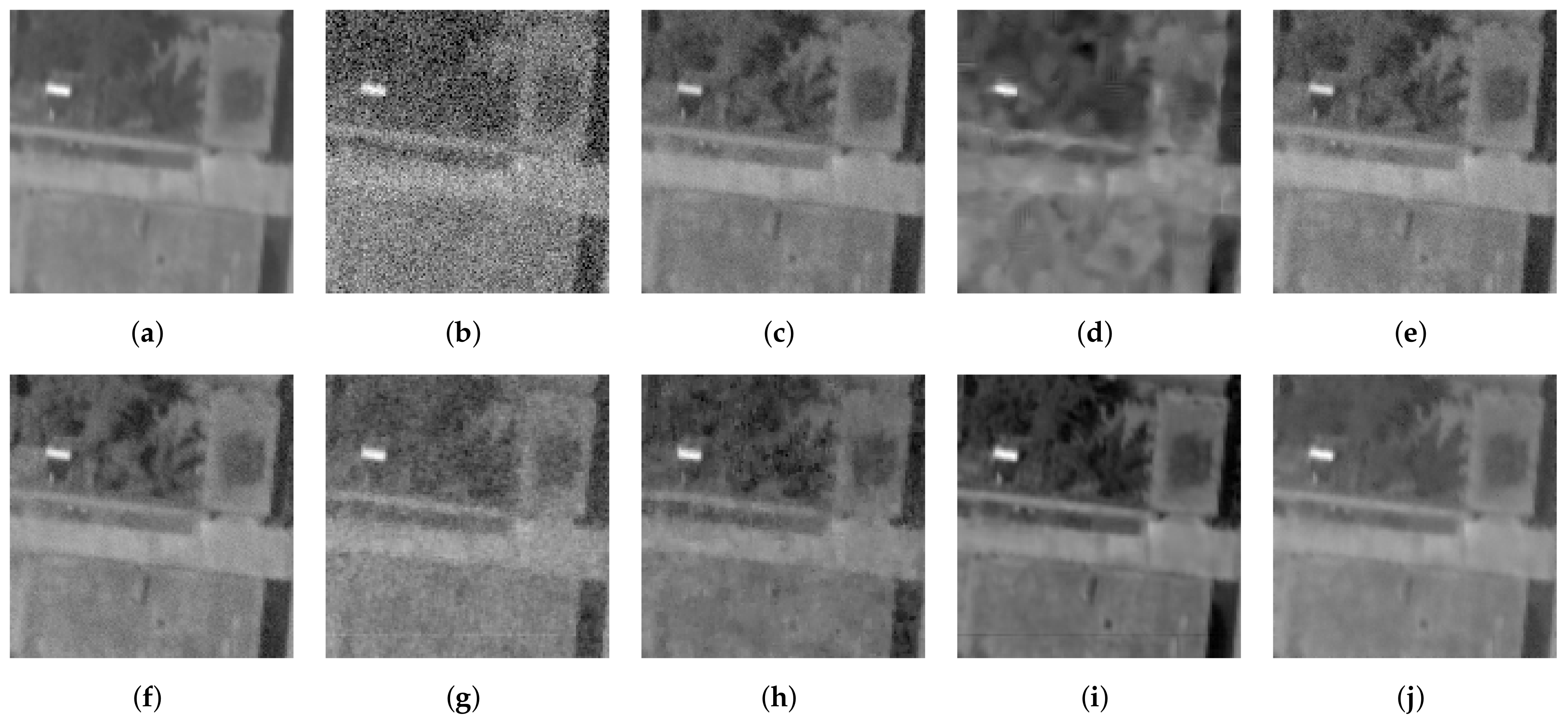
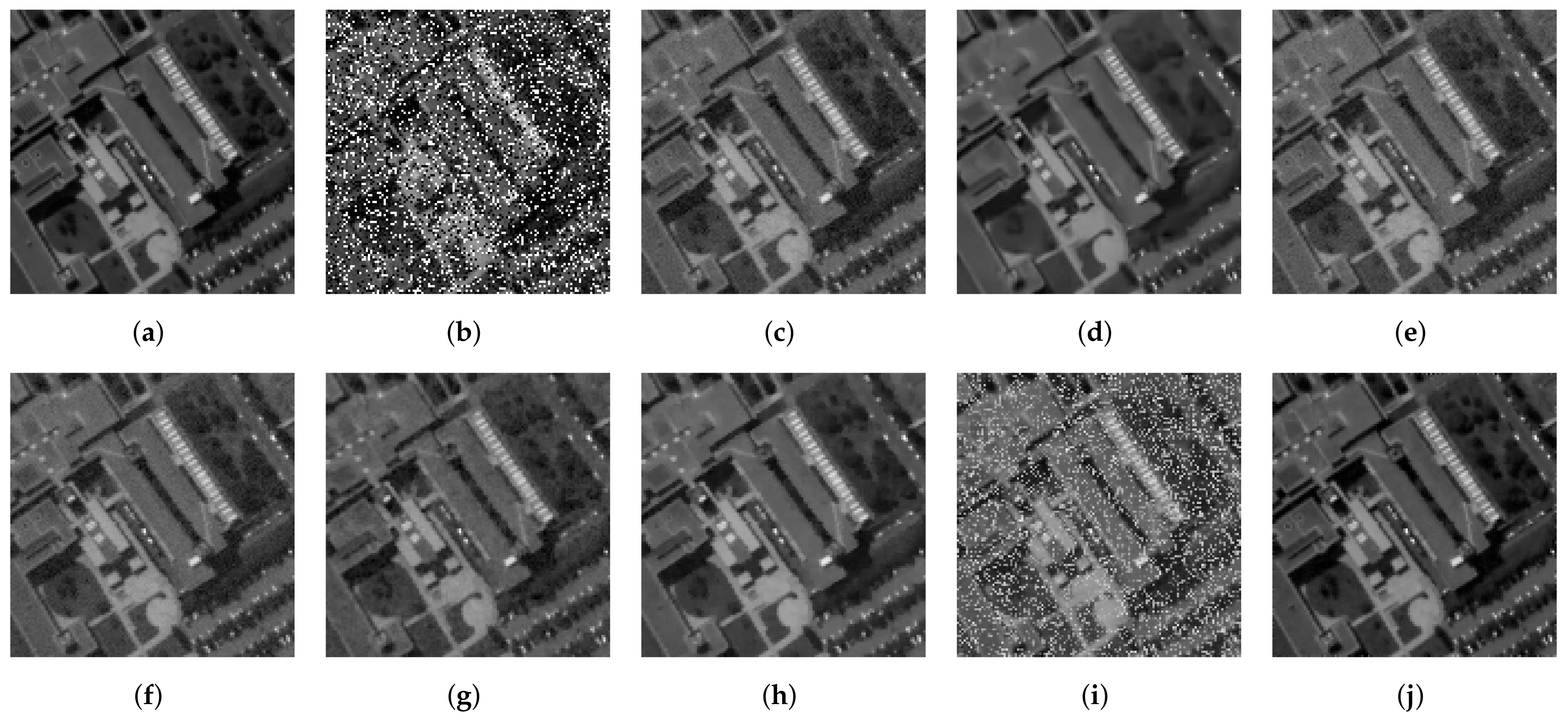
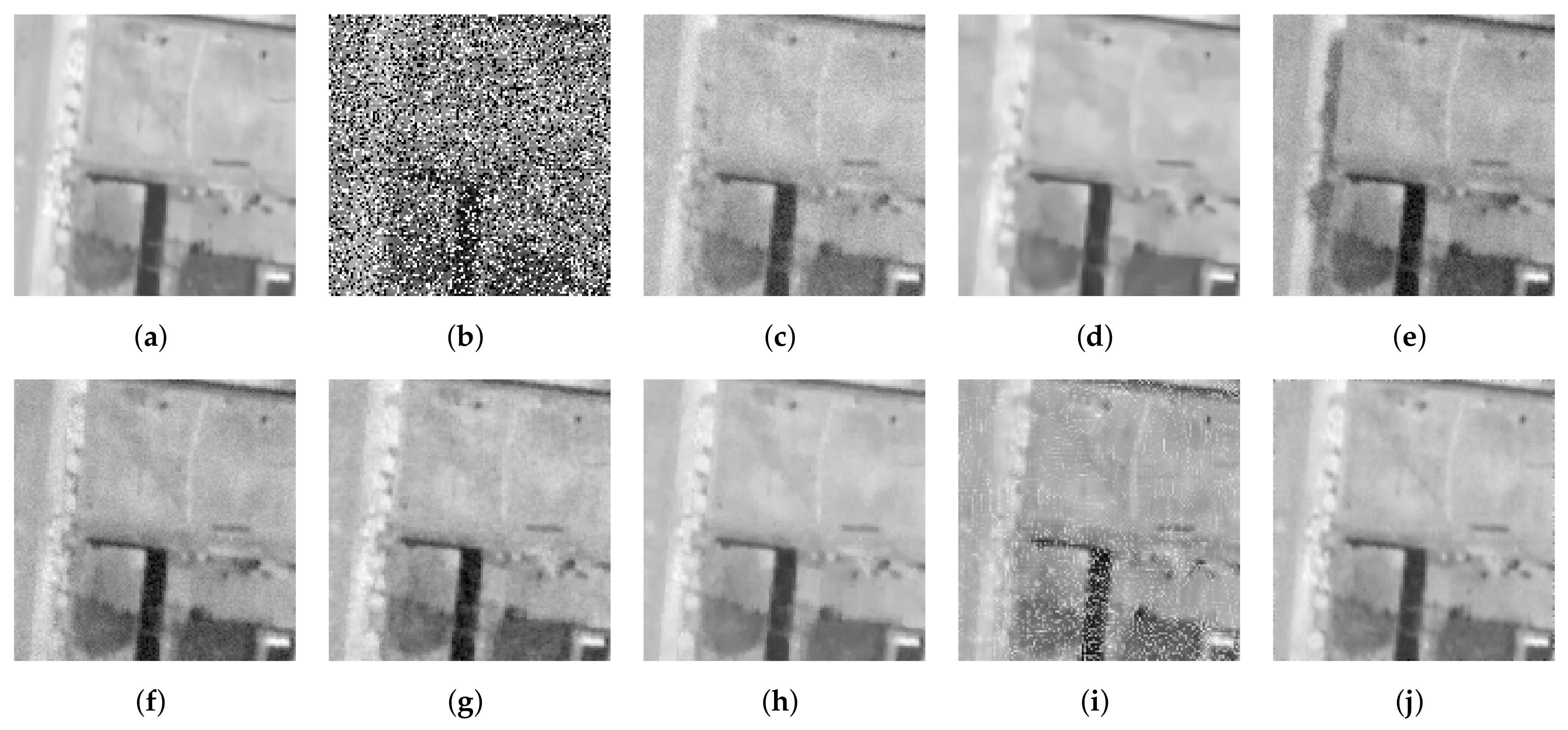
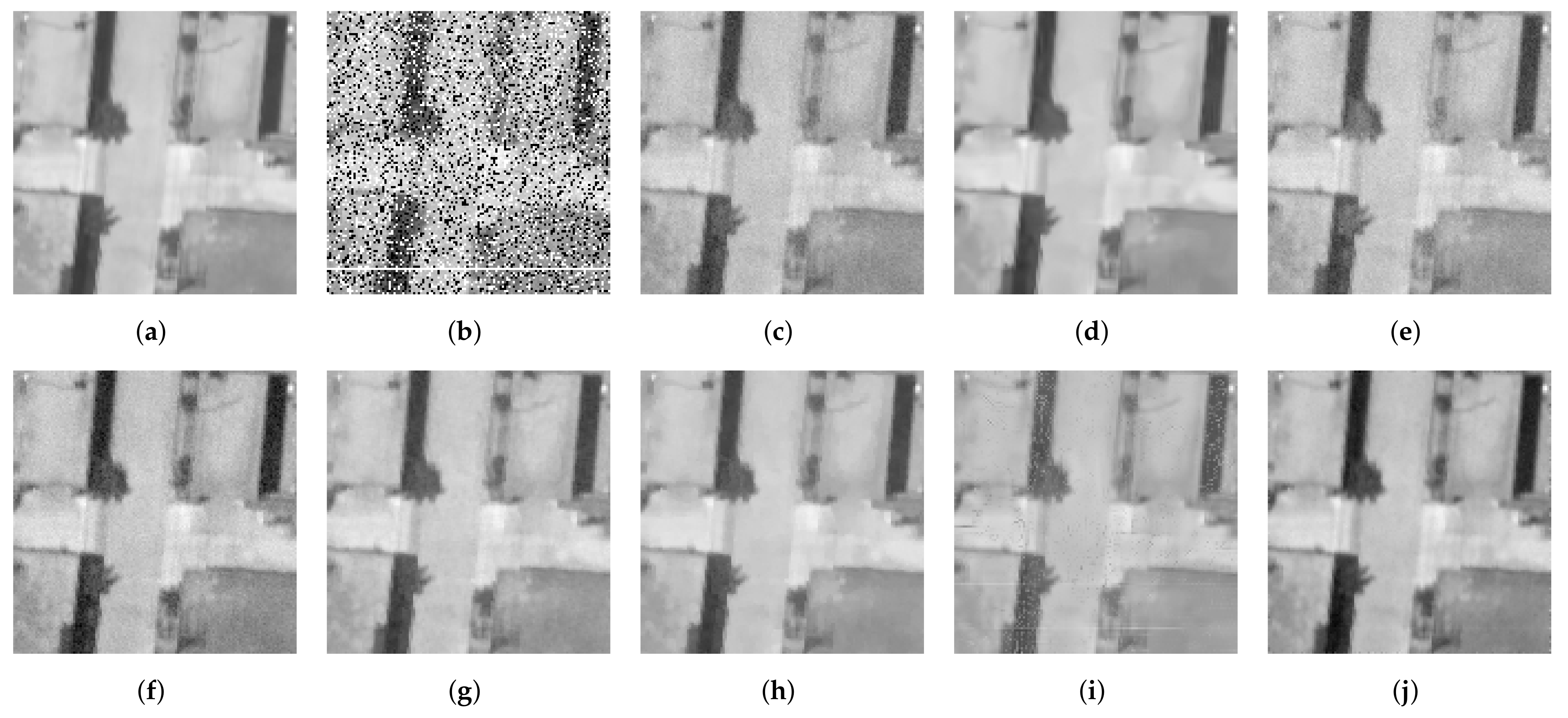
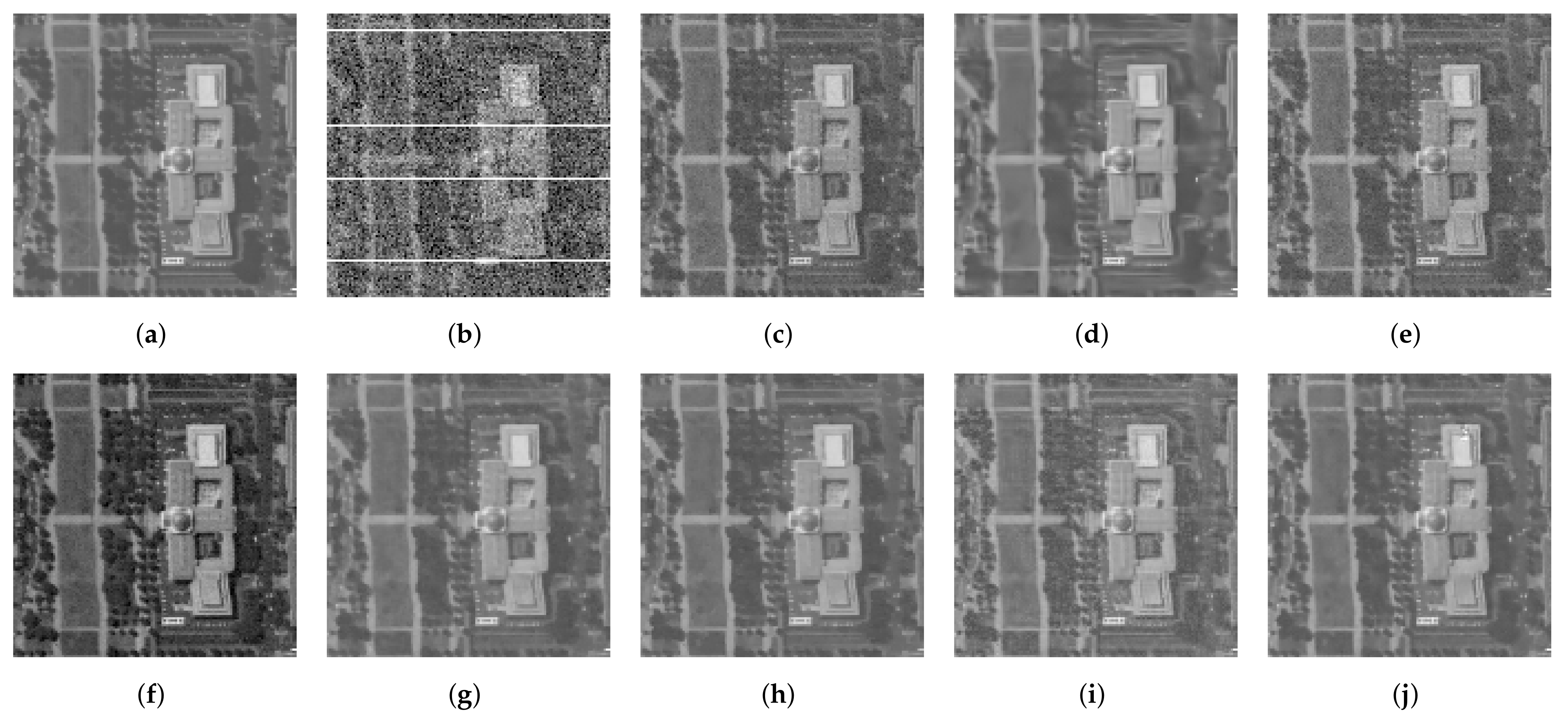
We performed comparative experiments on the SFD, Washington DC Mall, Pavia University and Xiongan New Area datasets. The detailed experimental results are shown in Table 1, in which the best performance for each noise case is marked in bold and the second best performance is underlined. Compared with these denoising methods, the proposed network achieves the highest MPSNR & MSSIM values, and the lowest MSAD values in most cases. We selected one HSI band in several noise cases to demonstrate the visual quality in Figure 5, Figure 6, Figure 7, Figure 8, Figure 9 and Figure 10, respectively.
In Figure 5, we can observe that Gaussian noise cannot be removed completely by NNM, WNNM, WSNM, LRTDTV and 3DTV, and that the generated images are blurred by BM4D. FastHyDe method suppresses the Gaussian noise better but brings the extra noise to the bottom of the image. The proposed method not only suppresses the Gaussian noise but also retains detailed image information.
As shown in Figure 6, although the FastHyDe method shows an effective noise reduction ability in handling the Gaussian noise, we found that the denoising image still contains the residual impulse noise. Similar results are observed from NNM, WNNM, WSNM and LRTDTV methods. Though other methods better manage suppress noise in this noise case, they often result in relatively low-quality indicators compared to the proposed method.
In Figure 7, the Gaussian noise cannot be completely removed by the NNM, WNNM, WSNM and LRTDTV methods and the FastHyDe method cannot remove impulse noise. In Figure 8, impulse noise and deadlines cannot be completely reduced by FastHyDe method, and Gaussian noise is still in the images denoised by the NNM, WNNM and WSNM methods. The proposed method achieves better performance compared with these existing methods.
In Figure 9, the noisy image suffered from the mixed noise, especially the high-intensity Gaussian noise. The NNM, WNNM and WSNM methods are ineffective given the complex noise distributions. The images denoised by the BM4D and FastHyDe methods still contain the slight stripe noise. In contrast with these, our proposed method can preserve the detailed image information, especially on the road part of the images.
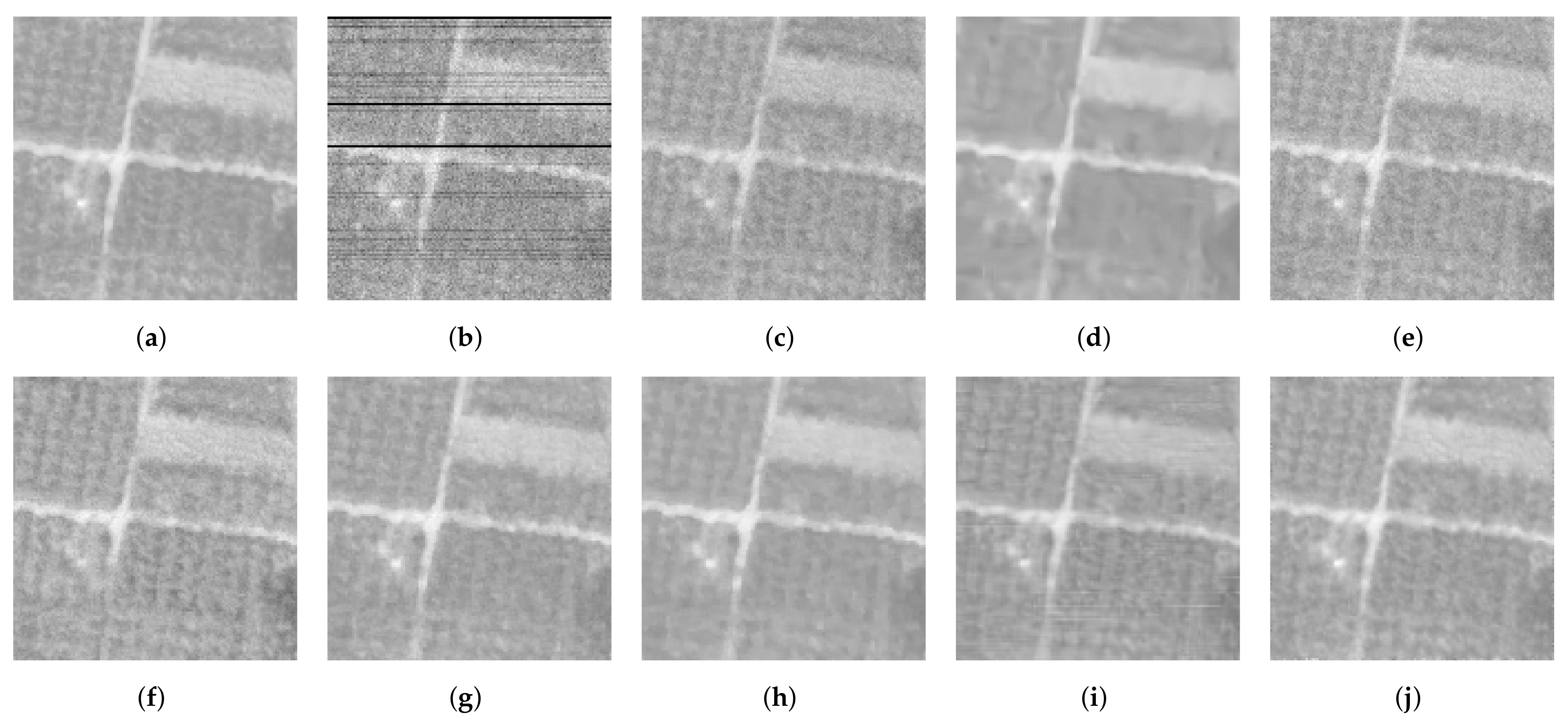
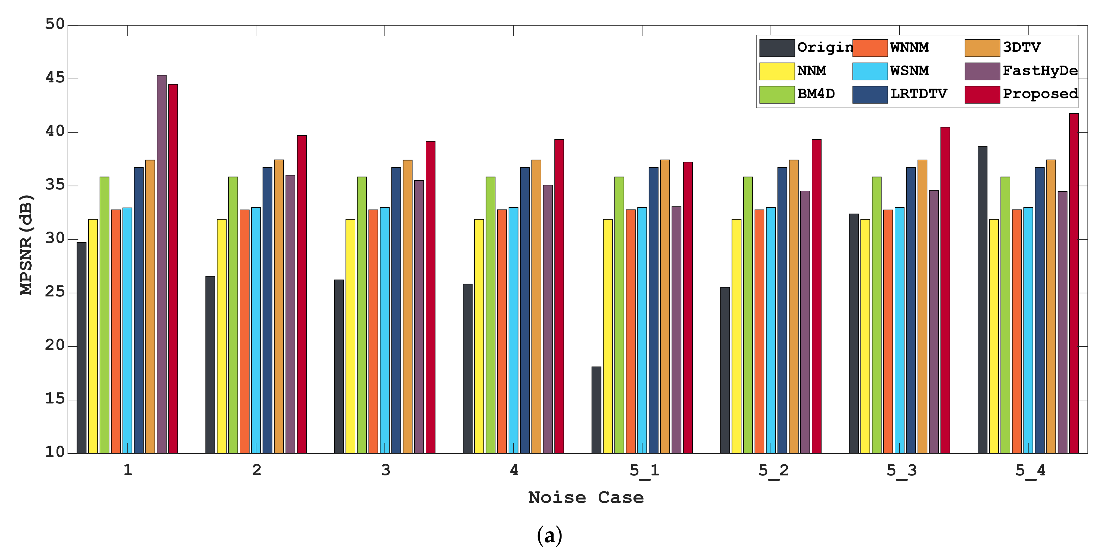
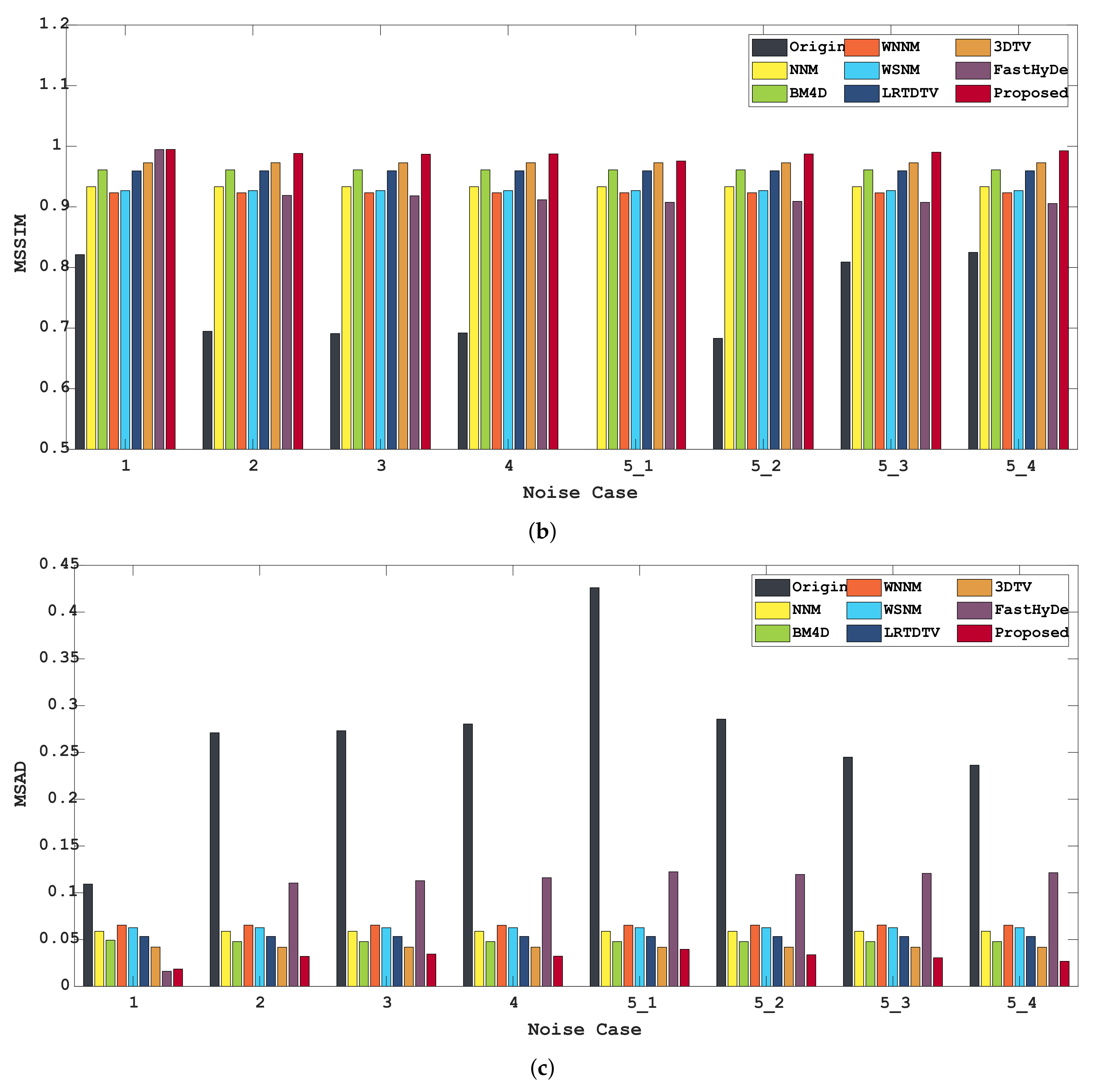
The denoising images of Case 5_2 are presented in Figure 10. The existing methods cannot completely remove the mixed noise. For example, the FastHyDe method performs less satisfactorily when dealing with the stripe noise and deadlines. Compared with these, the proposed denoising method achieves a significantly better performance in restoring the image details. To more clearly demonstrate the numerical results, Figure 11 shows the bar charts of the quantitative evaluation of different HSI denoising methods.
To discuss the denoising efficiency among wavebands, we selected Case 5_2 to show that the line charts of denoising efficiency vary with the waveband compared with existing methods on the SFD dataset in Figure 12. It can be observed that the denoising efficiency varies with the wavelength since the quality of each band in the original images is different. The indicators of the proposed model have the smallest fluctuation range compared with existing methods. For PSNR, the denoising indicator of the proposed model varies by approximately 3 dB. Furthermore, for SSIM, the denoising indicator of the proposed model varies less than 0.01. Moreover, the proposed model can attain higher MPSNR and MSSIM values for most wavebands.

3.4. Ablation Experiments

To validate the effectiveness of the proposed network, our ablation experiments were constituted of three aspects, including the network architecture, the joint loss functions and the amount of training data.
For the network architecture, we used the UNet-based architecture and improved the feature extraction by adding the RSSM residual blocks. Therefore, we compared UNet with and without the residual blocks as the generator in the first ablation experiment. To learn the noise distribution of the noisy images, we utilized the residual blocks instead of the double convolutional layers. We believe that residual learning can focus on the detailed differences between noisy images and noise-free images. Table 2 shows the first ablation experimental results, including the mean values and deviations in which the best performance for each noise case is marked in bold. As shown in Table 2, the quantitative indicators of the proposed network with residual learning are better in all mixed noise cases, proving that the residual blocks of UNet-based architecture are effective for the HSI denoising task.
For the loss function, we combined the reconstruction loss, the structural loss and the adversarial loss to jointly train the network with the total loss as L = λ r L r + λ s L s + λ a L a where we empirically set the λ r = 100 , λ s = 1 and λ a = 0.001 to keep the magnitude of different losses to the same level, which is a common practice in the neural network training with multiple losses. To further investigate the rationality and stability of the weight ratio, we conducted additional experiments by varying the ratio of the weights to the balanced and reversed order. Furthermore, we observed that the training process became much less optimal and even unstable, which demonstrates the importance of keeping the magnitude of losses at the same level. Moreover, the second ablation experiment was implemented by using single loss (Re/St/Ad) and two combined losses (Re + St/Re + Ad/St + Ad), respectively. Table 3 shows the second ablation experimental results, including mean values and deviations, in which the best performance for each noise case is marked in bold. We do not include the results of single loss St or Ad, and the combined loss St + Ad. This is because the reconstruction loss is crucial for obtaining a decent denoising effect as it minimizes the pixel-wise distance between generated images and noise-free images. The training without the reconstruction loss easily leads to divergency. It is observed that, in most mixed noise cases, the experimental results are gradually improved when the losses are added, proving that each loss plays a necessary role in improving the final performance of HSI denoising, especially with regard to the reconstruction loss.
For the amount of training data, we utilized 90% of the 3597 samples to train the proposed network. To further investigate the amount of training data required for the proposed model to start providing equivalent or even better results than the other methods compared, we conducted the third ablation experiment on the percentage of training data. We randomly selected 30%, 50% and 70% training data to train the proposed network with the same settings as in Case 5_2. The experimental results are shown in Table 4. Three line charts are plotted to demonstrate the results more clearly in Figure 13. From these results, we can find that with approximately 30% training data, the performance of our model already rivals those of compared methods, and more training data lead to results with higher denoising quality.

3.5. Experiments on Real Data

To further verify the effectiveness of the proposed network, Indian Pines, EO-1 Hyperion and Urban datasets were used in real-data experiments. The performance of the denoising was measured by the visual denoising images and mean digital number (DN) values.
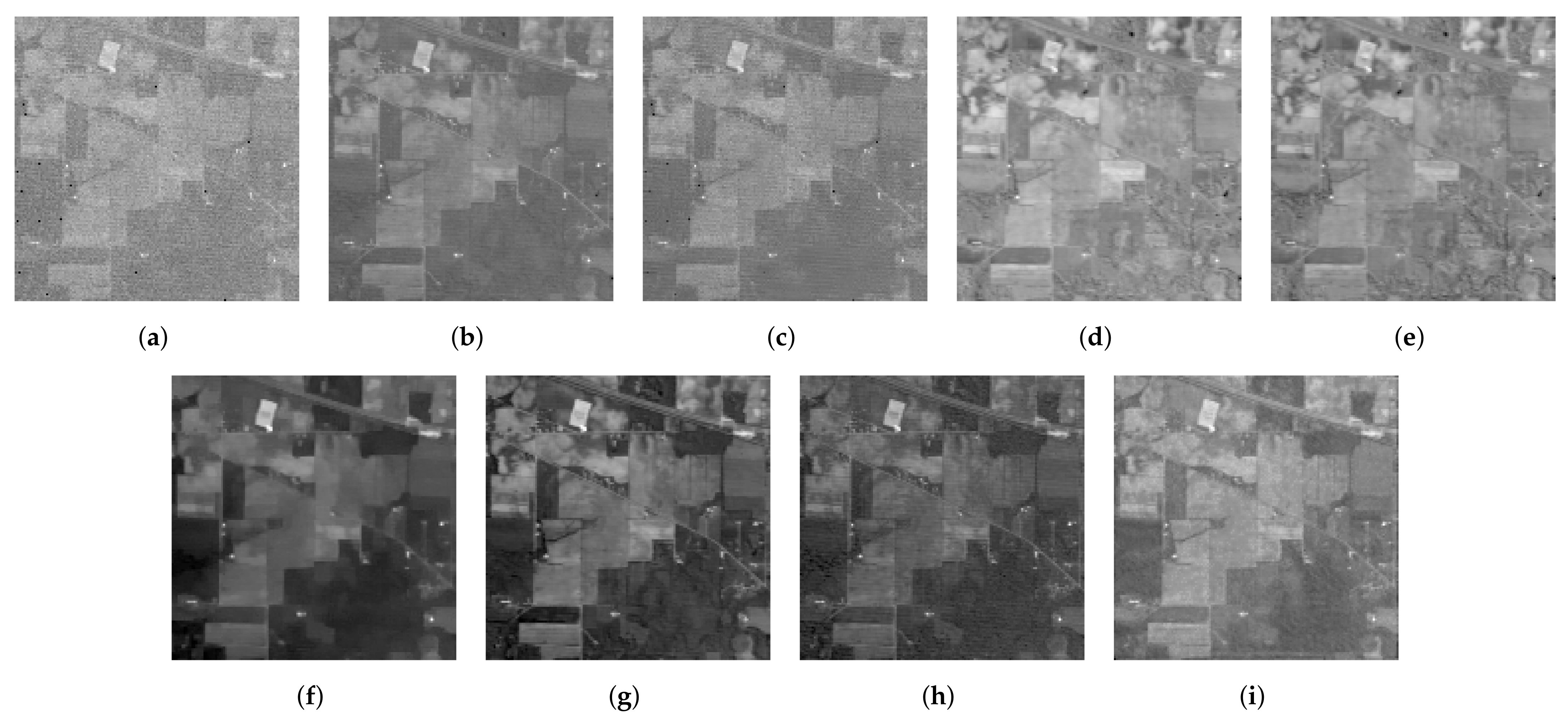
In the Indian Pines dataset, the first few bands and several of the middle bands suffered from Gaussian noise and impulse noise. We chose band 1 to show the denoising results of existing methods and the proposed method. Figure 14 shows the visual results of the denoising image on the Indian Pines dataset. It can be observed that Gaussian noise and impulse noise remain in the denoising image with the NNM, WNNM, WSNM and FastHyDe methods, and the BM4D method cannot remove the impulse noise in the original image. LRTDTV and 3DTV generate blurry images and lose some detailed information. The proposed method not only achieves the best performance on Gaussian and impulse noise removal but also maintains detailed information of the whole image.
In the Urban dataset, some middle bands strictly suffered from Gaussian noise, impulse noise, stripe noise and deadlines. We chose band 108 of the Urban dataset to demonstrate the visualized results against the compared methods. As shown in Figure 15, we observe that the original image of band 108 is severely degraded by the noise. The NNM, BM4D, WSNM, LRTDTV and FastHyDe methods cannot handle such mixed noise well, and there are still kinds of noise that remain in the processed images. Although the WNNM and 3DTV methods remove the mixed noise relatively well in the Urban dataset, the detailed information of the original image is simultaneously lost. Compared with these methods, the proposed model not only reduces the severe mixed noise but also maintains detailed image information.
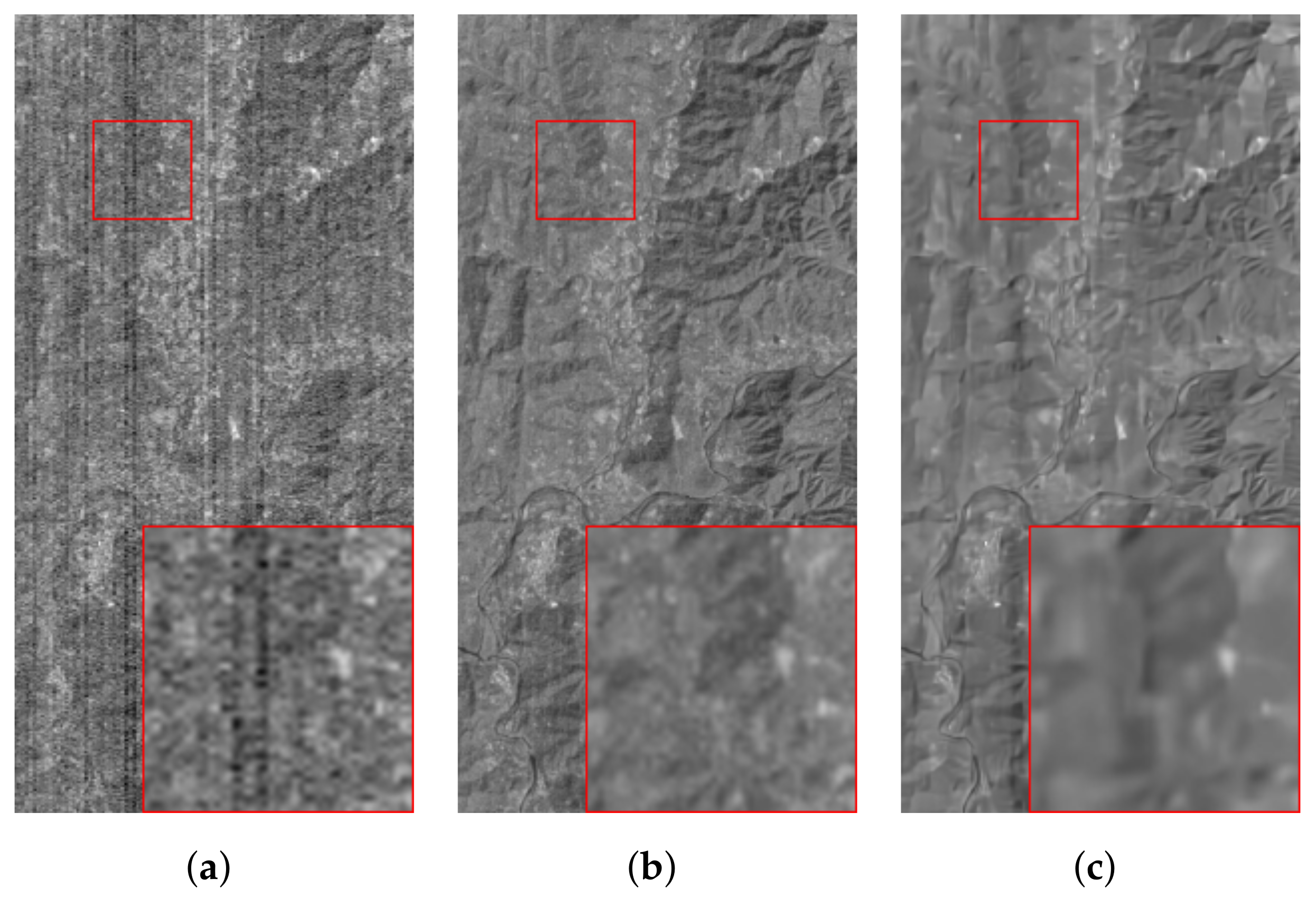
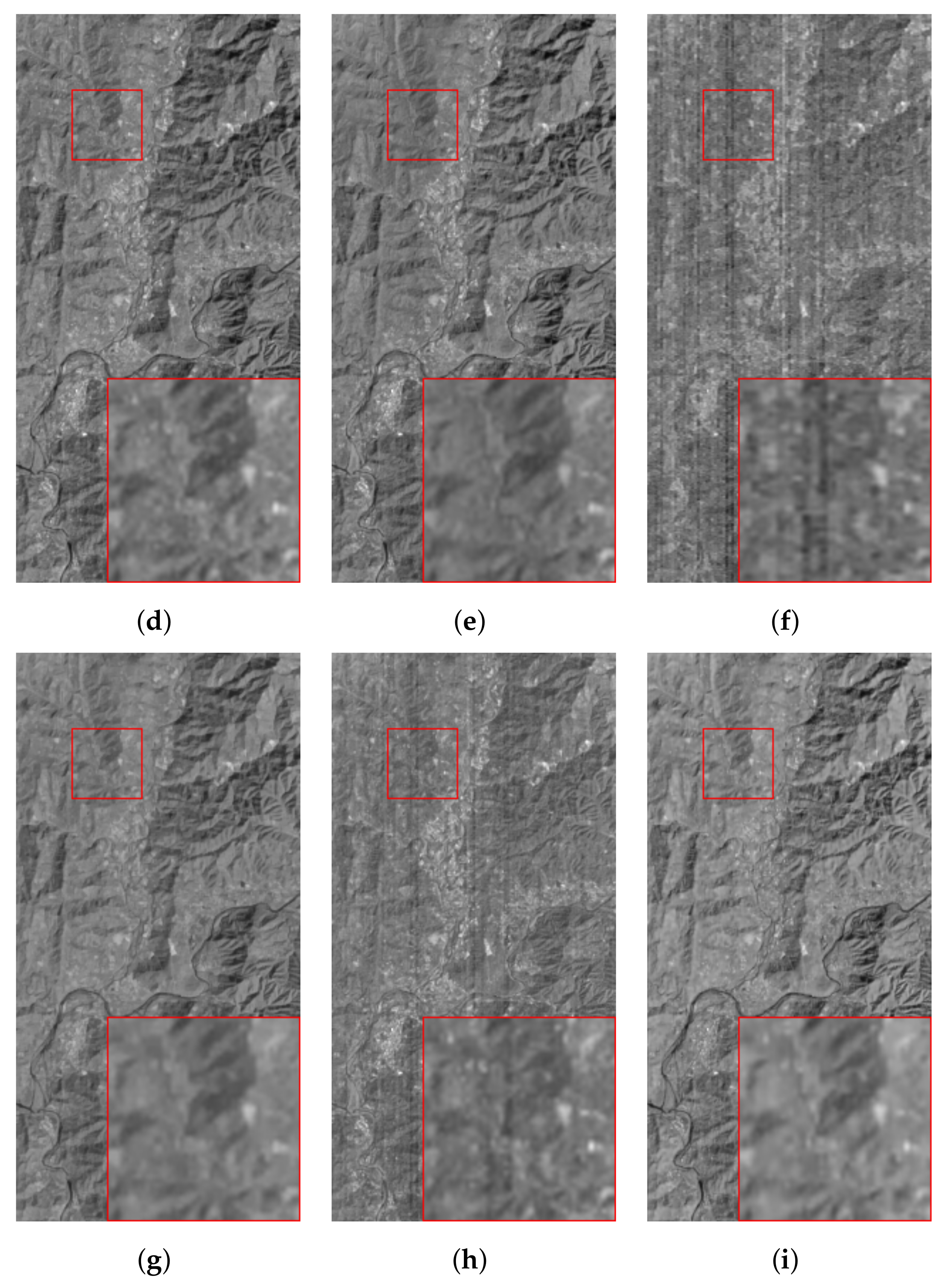
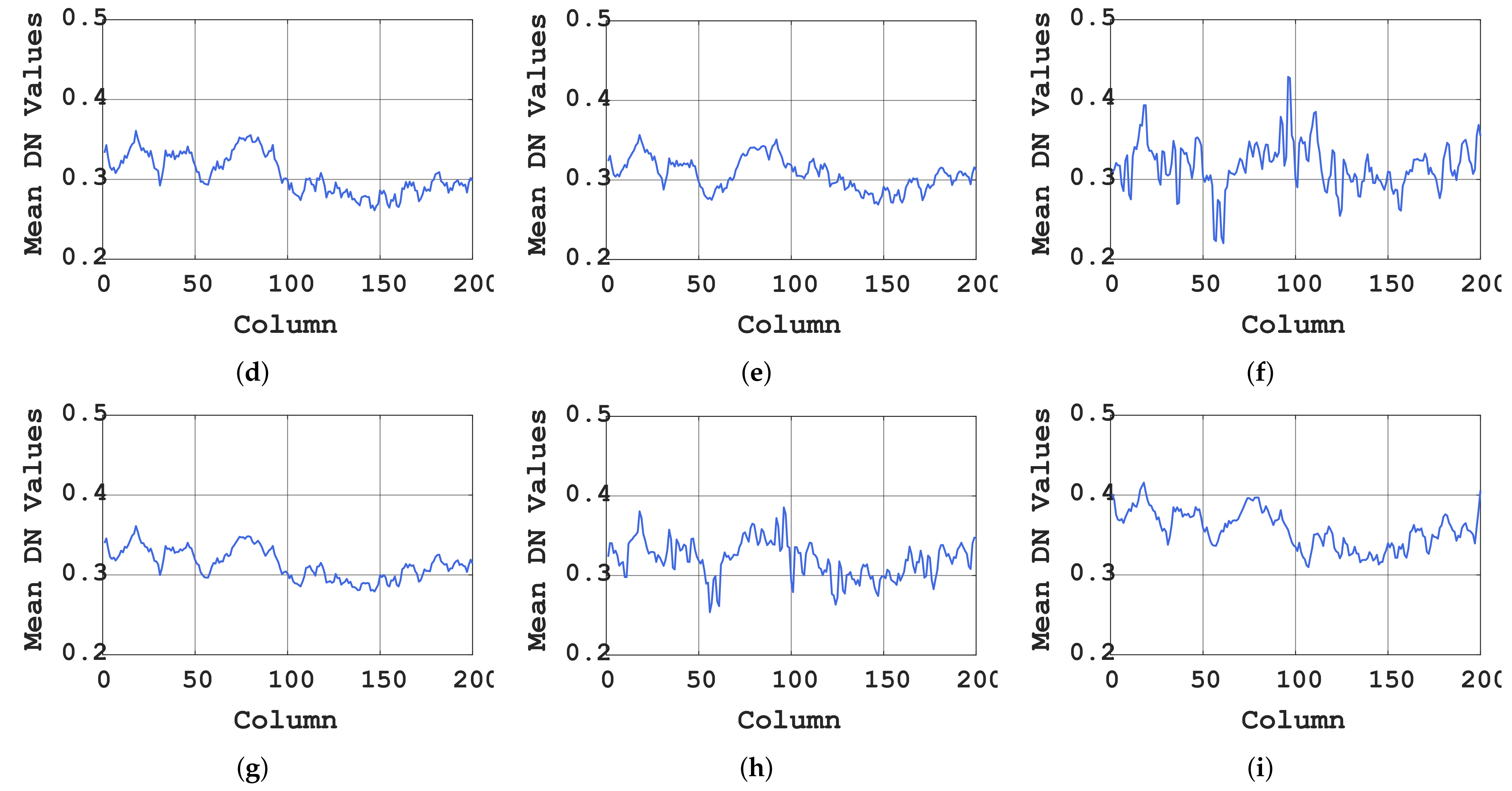
In the EO-1 Hyperion dataset, some of the bands are seriously affected by the Gaussian noise, stripe noise and deadlines. We chose band 36 to show the denoising results of the compared methods and proposed method. Figure 16 shows the visual results of the denoising image on the EO-1 Hyperion dataset, including partially enlarged details marked with red rectangles. As shown in Figure 16a, band 36 is corrupted by Gaussian noise, stripe noise and deadlines. In a remote sensing image, the DN values of pixels on the same column are often derived from the same detector pixel. Therefore, the smoothness of the vertical mean DN value curves represent the noise intensity of the images, especially for the stripe noise and deadlines. To evaluate the denoising performance and the detailed information reservation of HSIs, the vertical mean DN value curves are given in Figure 17. Although the BM4D, LRTDTV and FastHyDe methods can reduce certain noise, the mixed noise remains in the denoising images. The NNM, WNNM, WSNM and 3DTV methods can reduce most noise in the image yet lose the detailed information. Compared with the above methods, the proposed method achieves the best performance in reducing mixed noise while maintaining the local details.

4. Conclusions

In this paper, we propose an adversarial learning-based model for HSI denoising tasks, especially the mixed noise cases. The proposed network consists of a generator and a discriminator. For the generator, we improved the basic UNet structure by adding the RSSM to capture the noise distribution in the original HSIs instead of learning the direct mapping from noisy HSIs to noise-free HSIs. For the discriminator, a network with the MFFM was employed to extract the multiscale feature information to distinguish whether the generated HSIs were real or not. To focus on the structural similarity and reality of the generated images, joint loss functions are utilized during training including reconstruction loss, structural loss and adversarial loss.
We test five types of simulated noise cases including Gaussian noise, impulse noise, stripe noise, deadlines and their mixture. To evaluate the performance of the proposed network, we experiment on both public HSI datasets and the proposed SFD dataset. Comprehensive experiments including comparative experiments and ablation experiments verified the advantages of the proposed network against existing HSI denoising methods and the effectiveness of the proposed network. As for future work, we will further investigate the design of a light-weighted version of the proposed network architecture to maintain the model performance under constrained computation scenarios.

Author Contributions

Conceptualization, methodology, formal analysis and validation, J.Z. and Z.C.; investigation, software, visualization and writing—original draft preparation, Z.C.; data curation, F.C.; resources and supervision, J.Z. and D.Z.; writing—review and editing, J.Z., Z.C. and D.Z.; project administration and funding acquisition, D.Z. All authors have read and agreed to the published version of the manuscript.

Funding

This research was funded by the National Natural Science Foundation of China (No. 61572307).

Institutional Review Board Statement

Not applicable.

Informed Consent Statement

Not applicable.

Data Availability Statement

Public datasets are available at these links: http://www.ehu.eus/ccwintco/index.php/Hyperspectral_Remote_Sensing_Scenes (accessed on 24 February 2022), http://www.hrs-cas.com/a/share/shujuchanpin/2019/0501/1049.html (accessed on 24 February 2022) and https://engineering.purdue.edu/~biehl/MultiSpec/hyperspectral.html (accessed on 24 February 2022).

Conflicts of Interest

The authors declare no conflict of interest.

References

  1. Bioucas-Dias, J.M.; Plaza, A.; Camps-Valls, G.; Scheunders, P.; Nasrabadi, N.; Chanussot, J. Hyperspectral remote sensing data analysis and future challenges. IEEE Geosci. Remote Sens. Mag. 2013, 1, 6–36. [Google Scholar] [CrossRef] [Green Version]
  2. Chen, Y.; Lin, Z.; Zhao, X.; Wang, G.; Gu, Y. Deep learning-based classification of hyperspectral data. IEEE J. Sel. Top. Appl. Earth Obs. Remote Sens. 2014, 7, 2094–2107. [Google Scholar] [CrossRef]
  3. Chang, Y.L.; Tan, T.H.; Lee, W.H.; Chang, L.; Chen, Y.N.; Fan, K.C.; Alkhaleefah, M. Consolidated Convolutional Neural Network for Hyperspectral Image Classification. Remote Sens. 2022, 14, 1571. [Google Scholar] [CrossRef]
  4. Bioucas-Dias, J.M.; Plaza, A.; Dobigeon, N.; Parente, M.; Du, Q.; Gader, P.; Chanussot, J. Hyperspectral unmixing overview: Geometrical, statistical, and sparse regression-based approaches. IEEE J. Sel. Top. Appl. Earth Obs. Remote Sens. 2012, 5, 354–379. [Google Scholar] [CrossRef] [Green Version]
  5. Van Nguyen, H.; Banerjee, A.; Chellappa, R. Tracking via object reflectance using a hyperspectral video camera. In Proceedings of the 2010 IEEE Computer Society Conference on Computer Vision and Pattern Recognition-Workshops, San Francisco, CA, USA, 13–18 June 2010; pp. 44–51. [Google Scholar]
  6. Rasti, B.; Scheunders, P.; Ghamisi, P.; Licciardi, G.; Chanussot, J. Noise reduction in hyperspectral imagery: Overview and application. Remote Sens. 2018, 10, 482. [Google Scholar] [CrossRef] [Green Version]
  7. Dabov, K.; Foi, A.; Katkovnik, V.; Egiazarian, K. Image denoising by sparse 3-D transform-domain collaborative filtering. IEEE Trans. Image Process. 2007, 16, 2080–2095. [Google Scholar] [CrossRef]
  8. Gu, S.; Zhang, L.; Zuo, W.; Feng, X. Weighted nuclear norm minimization with application to image denoising. In Proceedings of the IEEE Conference on Computer Vision and Pattern Recognition, Columbus, OH, USA, 23–28 June 2014; pp. 2862–2869. [Google Scholar]
  9. Othman, H.; Qian, S.E. Noise reduction of hyperspectral imagery using hybrid spatial-spectral derivative-domain wavelet shrinkage. IEEE Trans. Geosci. Remote Sens. 2006, 44, 397–408. [Google Scholar] [CrossRef]
  10. Chen, G.; Qian, S.E. Simultaneous dimensionality reduction and denoising of hyperspectral imagery using bivariate wavelet shrinking and principal component analysis. Can. J. Remote Sens. 2008, 34, 447–454. [Google Scholar] [CrossRef]
  11. Yuan, Q.; Zhang, L.; Shen, H. Hyperspectral image denoising employing a spectral–spatial adaptive total variation model. IEEE Trans. Geosci. Remote Sens. 2012, 50, 3660–3677. [Google Scholar] [CrossRef]
  12. Maggioni, M.; Katkovnik, V.; Egiazarian, K.; Foi, A. Nonlocal transform-domain filter for volumetric data denoising and reconstruction. IEEE Trans. Image Process. 2012, 22, 119–133. [Google Scholar] [CrossRef]
  13. He, W.; Zhang, H.; Zhang, L.; Shen, H. Total-variation-regularized low-rank matrix factorization for hyperspectral image restoration. IEEE Trans. Geosci. Remote Sens. 2015, 54, 178–188. [Google Scholar] [CrossRef]
  14. Liu, X.; Bourennane, S.; Fossati, C. Denoising of hyperspectral images using the PARAFAC model and statistical performance analysis. IEEE Trans. Geosci. Remote Sens. 2012, 50, 3717–3724. [Google Scholar] [CrossRef]
  15. Peng, Y.; Meng, D.; Xu, Z.; Gao, C.; Yang, Y.; Zhang, B. Decomposable nonlocal tensor dictionary learning for multispectral image denoising. In Proceedings of the IEEE Conference on Computer Vision and Pattern Recognition, Columbus, OH, USA, 23–28 June 2014; pp. 2949–2956. [Google Scholar]
  16. Wang, Y.; Peng, J.; Zhao, Q.; Leung, Y.; Zhao, X.L.; Meng, D. Hyperspectral image restoration via total variation regularized low-rank tensor decomposition. IEEE J. Sel. Top. Appl. Earth Obs. Remote Sens. 2017, 11, 1227–1243. [Google Scholar] [CrossRef] [Green Version]
  17. Fan, H.; Li, C.; Guo, Y.; Kuang, G.; Ma, J. Spatial–spectral total variation regularized low-rank tensor decomposition for hyperspectral image denoising. IEEE Trans. Geosci. Remote Sens. 2018, 56, 6196–6213. [Google Scholar] [CrossRef]
  18. Xie, W.; Li, Y. Hyperspectral imagery denoising by deep learning with trainable nonlinearity function. IEEE Geosci. Remote Sens. Lett. 2017, 14, 1963–1967. [Google Scholar] [CrossRef]
  19. Yuan, Q.; Zhang, Q.; Li, J.; Shen, H.; Zhang, L. Hyperspectral image denoising employing a spatial–spectral deep residual convolutional neural network. IEEE Trans. Geosci. Remote Sens. 2018, 57, 1205–1218. [Google Scholar] [CrossRef] [Green Version]
  20. Ronneberger, O.; Fischer, P.; Brox, T. U-net: Convolutional networks for biomedical image segmentation. In Proceedings of the International Conference on Medical Image Computing and Computer-Assisted Intervention, Munich, Germany, 5–9 October 2015; Springer: Berlin/Heidelberg, Germany, 2015; pp. 234–241. [Google Scholar]
  21. Dong, W.; Wang, H.; Wu, F.; Shi, G.; Li, X. Deep spatial–spectral representation learning for hyperspectral image denoising. IEEE Trans. Comput. Imaging 2019, 5, 635–648. [Google Scholar] [CrossRef]
  22. Zhang, Q.; Yuan, Q.; Li, J.; Liu, X.; Shen, H.; Zhang, L. Hybrid noise removal in hyperspectral imagery with a spatial–spectral gradient network. IEEE Trans. Geosci. Remote Sens. 2019, 57, 7317–7329. [Google Scholar] [CrossRef]
  23. Goodfellow, I.; Pouget-Abadie, J.; Mirza, M.; Xu, B.; Warde-Farley, D.; Ozair, S.; Courville, A.; Bengio, Y. Generative adversarial nets. In Proceedings of the Advances in Neural Information Processing Systems, Montreal, QC, USA, 8–13 December 2014; Volume 27. [Google Scholar]
  24. Gulrajani, I.; Ahmed, F.; Arjovsky, M.; Dumoulin, V.; Courville, A. Improved training of wasserstein gans. arXiv 2017, arXiv:1704.00028. [Google Scholar]
  25. Ledig, C.; Theis, L.; Huszár, F.; Caballero, J.; Cunningham, A.; Acosta, A.; Aitken, A.; Tejani, A.; Totz, J.; Wang, Z.; et al. Photo-realistic single image super-resolution using a generative adversarial network. In Proceedings of the IEEE Conference on Computer Vision and Pattern Recognition, Honolulu, HI, USA, 21–26 July 2017; pp. 4681–4690. [Google Scholar]
  26. Radford, A.; Metz, L.; Chintala, S. Unsupervised representation learning with deep convolutional generative adversarial networks. arXiv 2015, arXiv:1511.06434. [Google Scholar]
  27. Yang, Q.; Yan, P.; Zhang, Y.; Yu, H.; Shi, Y.; Mou, X.; Kalra, M.K.; Zhang, Y.; Sun, L.; Wang, G. Low-dose CT image denoising using a generative adversarial network with Wasserstein distance and perceptual loss. IEEE Trans. Med. Imaging 2018, 37, 1348–1357. [Google Scholar] [CrossRef] [PubMed]
  28. Wolterink, J.M.; Leiner, T.; Viergever, M.A.; Išgum, I. Generative adversarial networks for noise reduction in low-dose CT. IEEE Trans. Med. Imaging 2017, 36, 2536–2545. [Google Scholar] [CrossRef] [PubMed]
  29. Chen, Z.; Zeng, Z.; Shen, H.; Zheng, X.; Dai, P.; Ouyang, P. DN-GAN: Denoising generative adversarial networks for speckle noise reduction in optical coherence tomography images. Biomed. Signal Process. Control 2020, 55, 101632. [Google Scholar] [CrossRef]
  30. Lyu, Q.; Guo, M.; Pei, Z. DeGAN: Mixed noise removal via generative adversarial networks. Appl. Soft Comput. 2020, 95, 106478. [Google Scholar] [CrossRef]
  31. Chen, S.; Shi, D.; Sadiq, M.; Cheng, X. Image Denoising With Generative Adversarial Networks and its Application to Cell Image Enhancement. IEEE Access 2020, 8, 82819–82831. [Google Scholar] [CrossRef]
  32. He, K.; Zhang, X.; Ren, S.; Sun, J. Deep residual learning for image recognition. In Proceedings of the IEEE Conference on Computer Vision and Pattern Recognition, Las Vegas, NV, USA, 27–30 June 2016; pp. 770–778. [Google Scholar]
  33. Isola, P.; Zhu, J.Y.; Zhou, T.; Efros, A.A. Image-to-image translation with conditional adversarial networks. In Proceedings of the IEEE Conference on Computer Vision and Pattern Recognition, Honolulu, HI, USA, 21–26 July 2017; pp. 1125–1134. [Google Scholar]
  34. Wang, Z.; Bovik, A.C.; Sheikh, H.R.; Simoncelli, E.P. Image quality assessment: From error visibility to structural similarity. IEEE Trans. Image Process. 2004, 13, 600–612. [Google Scholar] [CrossRef] [Green Version]
  35. Kingma, D.P.; Ba, J. Adam: A method for stochastic optimization. arXiv 2014, arXiv:1412.6980. [Google Scholar]
  36. Cen, Y.; Zhang, L.; Zhang, X.; Wang, Y.; Qi, W.; Tang, S.; Zhang, P. Aerial hyperspectral remote sensing classification dataset of Xiongan New Area (Matiwan Village). J. Remote Sens. 2020, 24, 1299–1306. [Google Scholar]
  37. Peng, J.; Xie, Q.; Zhao, Q.; Wang, Y.; Meng, D.; Leung, Y. Enhanced 3DTV regularization and its applications on hyper-spectral image denoising and compressed sensing. arXiv 2018, arXiv:1809.06591. [Google Scholar]
  38. Wei, K.; Fu, Y.; Huang, H. 3-D quasi-recurrent neural network for hyperspectral image denoising. IEEE Trans. Neural Netw. Learn. Syst. 2020, 32, 363–375. [Google Scholar] [CrossRef] [Green Version]
  39. Wright, J.; Ganesh, A.; Rao, S.R.; Peng, Y.; Ma, Y. Robust principal component analysis: Exact recovery of corrupted low-rank matrices via convex optimization. In Proceedings of the Advances in Neural Information Processing Systems, Vancouver, BC, Canada, 7–10 December 2009; Volume 58, pp. 289–298. [Google Scholar]
  40. Xie, Y.; Qu, Y.; Tao, D.; Wu, W.; Yuan, Q.; Zhang, W. Hyperspectral image restoration via iteratively regularized weighted schatten p-norm minimization. IEEE Trans. Geosci. Remote Sens. 2016, 54, 4642–4659. [Google Scholar] [CrossRef]
  41. Zhuang, L.; Bioucas-Dias, J.M. Fast hyperspectral image denoising and inpainting based on low-rank and sparse representations. IEEE J. Sel. Top. Appl. Earth Obs. Remote Sens. 2018, 11, 730–742. [Google Scholar] [CrossRef]
Figure 1. The proposed network architecture including the generator and the discriminator. The noisy HSIs are fed to the generator, and the denoising HSIs are then generated and fed to the discriminator. The discriminator learns to distinguish whether the input HSIs are from the generator or ground truth. The generator intends to generate more realistic HSIs to deceive the discriminator.
Remotesensing 14 01790 g001
Figure 2. The architecture of the Residual Spatial-Spectral Module, where h, w and c represent the sizes of the feature maps and the kernel size of each convolutional layer is marked out.
Remotesensing 14 01790 g002
Figure 3. The architecture of Multiscale Feature Fusion Module, where h, w and c represent the sizes of feature maps and the kernel size of each convolutional layer is marked out.
Remotesensing 14 01790 g003
Figure 4. Shandong Feicheng Denoising (SFD) dataset: (a) farmland; (b) building; (c) dirt; (d) lake; (e) road; and (f) tree.
Remotesensing 14 01790 g004
Figure 5. Case 1: The comparison of hyperspectral images (HSIs) denoising results with existing methods on the SFD dataset: (a) ground truth of band 3; (b) noisy image; (c) NNM; (d) BM4D; (e) WNNM; (f) WSNM; (g) LRTDTV; (h) 3DTV; (i) FastHyDel and (j) the proposed method.
Remotesensing 14 01790 g005
Figure 6. Case 2: The comparison of HSIs denoising results with existing methods on the Pavia University dataset: (a) ground truth of band 27; (b) noisy image; (c) NNM; (d) BM4D; (e) WNNM; (f) WSNM; (g) LRTDTV; (h) 3DTV; (i) FastHyDe; and (j) the proposed method.
Remotesensing 14 01790 g006
Figure 7. Case 3: The comparison of HSIs denoising results with existing methods on the SFD dataset: (a) ground truth of band 35; (b) noisy image; (c) NNM; (d) BM4D; (e) WNNM; (f) WSNM; (g) LRTDTV; (h) 3DTV; (i) FastHyDe; and (j) the proposed method.
Remotesensing 14 01790 g007
Figure 8. Case 4: The comparison of HSIs denoising results with existing methods on the SFD dataset: (a) ground truth of band 21; (b) noisy image; (c) NNM; (d) BM4D; (e) WNNM; (f) WSNM; (g) LRTDTV; (h) 3DTV; (i) FastHyDe; and (j) the proposed method.
Remotesensing 14 01790 g008
Figure 9. Case 5_1: The comparison of HSIs denoising results with existing methods on the Washington DC Mall dataset: (a) ground truth of band 18; (b) noisy image; (c) NNM; (d) BM4D; (e) WNNM; (f) WSNM; (g) LRTDTV; (h) 3DTV; (i) FastHyDe; and (j) the proposed method.
Remotesensing 14 01790 g009
Figure 10. Case 5_2: The comparison of HSIs denoising results with existing methods on the Xiongan New Area dataset: (a) ground truth of band 15; (b) noisy image; (c) NNM; (d) BM4D; (e) WNNM; (f) WSNM; (g) LRTDTV; (h) 3DTV; (i) FastHyDe; and (j) the proposed method.
Remotesensing 14 01790 g010
Figure 11. The bar charts of the quantitative evaluation of different HSI denoising methods on five noise cases: (a) MPSNR (dB); (b) MSSIM; and (c) MSAD.
Remotesensing 14 01790 g011aRemotesensing 14 01790 g011b
Figure 12. The line charts of the denoising efficiency vary with the waveband compared with existing methods on the SFD dataset (Case 5_2): (a) PSNR (dB); and (b) SSIM.
Remotesensing 14 01790 g012
Figure 13. The line charts of the percentage of training samples and indicators (Case 5_2): (a) MPSNR (dB); (b) MSSIM; and (c) MSAD.
Remotesensing 14 01790 g013
Figure 14. Real-data experiments of HSI denoising results against existing methods on the Indian Pines dataset: (a) original image of band 1; (b) NNM; (c) BM4D; (d) WNNM; (e) WSNM; (f) LRTDTV; (g) 3DTV; (h) FastHyDe; and (i) the proposed method.
Remotesensing 14 01790 g014
Figure 15. Real-data experiments of HSI denoising results against existing methods on the Urban dataset: (a) original image of band 108; (b) NNM; (c) BM4D; (d) WNNM; (e) WSNM; (f) LRTDTV; (g) 3DTV; (h) FastHyDe; and (i) the proposed method.
Remotesensing 14 01790 g015aRemotesensing 14 01790 g015b
Figure 16. Real-data experiment of HSI denoising results compared with existing methods on the EO-1 Hyperion dataset: (a) original image of band 36; (b) NNM; (c) BM4D; (d) WNNM; (e) WSNM; (f) LRTDTV; (g) 3DTV; (h) FastHyDe; and (i) the proposed method.
Remotesensing 14 01790 g016aRemotesensing 14 01790 g016b
Figure 17. Vertical mean DN value on the EO-1 Hyperion dataset: (a) original image of band 36; (b) NNM; (c) BM4D; (d) WNNM; (e) WSNM; (f) LRTDTV; (g) 3DTV; (h) FastHyDe; and (i) the proposed method.
Remotesensing 14 01790 g017aRemotesensing 14 01790 g017b
Table 1. Quantitative evaluation of the denoising results of different methods on five noise cases.
Noise CaseIndexNoisyNNMBM4DWNNMWSNMLRTDTV3DTVFastHyDeProposed
Case 1MPSNR29.718331.880235.839332.768332.956236.720237.418645.346344.4981
MSSIM0.82120.93320.96100.92320.92680.95930.97270.99450.9947
MSAD0.10930.05880.04930.06540.06270.05330.04200.01610.0185
Case 2MPSNR26.561031.880535.839532.764332.980936.726137.440236.007339.7086
MSSIM0.69470.93320.96100.92320.92680.95950.97280.91890.9882
MSAD0.27100.05880.04790.06540.06270.05340.04180.11040.0321
Case 3MPSNR26.229131.879635.839132.768732.985936.723637.413735.512839.1681
MSSIM0.69100.93330.96100.92330.92690.95950.97270.91820.9869
MSAD0.27320.05890.04790.06540.06260.05340.04190.11290.0345
Case 4MPSNR25.833431.879435.838232.775032.984236.726837.425935.076439.3436
MSSIM0.69200.93320.96100.92330.92680.95950.97280.91170.9874
MSAD0.28040.05890.04790.06530.06270.05340.04190.11610.0322
Case 5_1MPSNR18.107631.879135.838232.774632.984436.724637.437933.062437.2248
MSSIM0.31740.93320.96100.92330.92680.95950.97280.90750.9756
MSAD0.42600.05890.04790.06530.06270.05340.04180.12240.0396
Case 5_2MPSNR25.536531.880335.838732.769132.985336.724537.424034.528039.3337
MSSIM0.68310.93330.96100.92320.92690.95950.97270.90910.9872
MSAD0.28560.05890.04790.06540.06270.05330.04190.11960.0338
Case 5_3MPSNR32.387131.877935.839132.760332.984536.721737.431634.591840.4928
MSSIM0.80900.93330.96100.92310.92690.95950.97270.90740.9902
MSAD0.24490.05890.04790.06550.06270.05330.04190.12080.0305
Case 5_4MPSNR38.676831.877435.838932.775032.984236.724037.439034.481941.7679
MSSIM0.82490.93330.96100.92330.92680.95950.97270.90550.9925
MSAD0.23640.05890.04790.06530.06270.05330.04180.12150.0268
Table 2. Quantitative evaluation of the ablation experiment on the SFD dataset: architecture.
Noise CaseIndexOriginU-NetProposed
Case 1MPSNR29.806730.9705 ± 0.016444.9872 ± 0.0697
MSSIM0.82840.8602 ± 0.00030.9957 ± 0.0002
MSAD0.11210.0987 ± 0.00010.0176 ± 0.0001
Case 2MPSNR26.611537.2653 ± 0.071239.9983 ± 0.0625
MSSIM0.69670.9788 ± 0.00030.9895 ± 0.0002
MSAD0.28230.0431 ± 0.00040.0313 ± 0.0004
Case 3MPSNR26.276436.4807 ± 0.064639.1705 ± 0.0562
MSSIM0.69670.9772 ± 0.00070.9877 ± 0.0003
MSAD0.28230.0446 ± 0.00060.0356 ± 0.0004
Case 4MPSNR25.888636.2525 ± 0.092839.3835 ± 0.0762
MSSIM0.69830.9766 ± 0.00040.9881 ± 0.0003
MSAD0.29000.0457 ± 0.00080.0318 ± 0.0003
Case 5_1MPSNR18.270034.8893 ± 0.087737.6784 ± 0.0163
MSSIM0.32810.9678 ± 0.00070.9793 ± 0.0003
MSAD0.43300.0486 ± 0.00080.0387 ± 0.0004
Case 5_2MPSNR25.590436.3373 ± 0.041239.5645 ± 0.0421
MSSIM0.68920.9725 ± 0.00020.9883 ± 0.0001
MSAD0.29450.0459 ± 0.00030.0333 ± 0.0005
Case 5_3MPSNR32.406337.0978 ± 0.097940.6836 ± 0.0794
MSSIM0.81000.9832 ± 0.00060.9908 ± 0.0003
MSAD0.25370.0401 ± 0.00110.0301 ± 0.0006
Case 5_4MPSNR38.690938.7968 ± 0.066941.9246 ± 0.0590
MSSIM0.82480.9862 ± 0.00080.9930 ± 0.0002
MSAD0.24380.0383 ± 0.00060.0263 ± 0.0002
Table 3. Quantitative evaluation of the ablation experiment on the SFD dataset: loss functions. Re means the reconstruction loss; St means the structural loss; and Ad means the adversarial loss.
Noise CaseIndexOriginReRe + StRe+AdRe + St + Ad
Case 1MPSNR29.806743.4532 ± 0.089644.5108 ± 0.090344.691 ± 0.064944.9872 ± 0.0697
MSSIM0.82840.9950 ± 0.00020.9956 ± 0.00000.9957 ± 0.00000.9957 ± 0.0002
MSAD0.11210.0228 ± 0.00020.0193 ± 0.00020.0185 ± 0.00010.0176 ± 0.0001
Case 2MPSNR26.611537.0614 ± 0.076839.7972 ± 0.075239.9942 ± 0.057539.9983 ± 0.0625
MSSIM0.69670.9834 ± 0.00360.9892 ± 0.00020.9885 ± 0.00020.9895 ± 0.0002
MSAD0.28230.0514 ± 0.00120.0327 ± 0.00030.0311 ± 0.00040.0313 ± 0.0004
Case 3MPSNR26.276436.6589 ± 0.064138.9176 ± 0.054238.9326 ± 0.054739.1705 ± 0.0562
MSSIM0.69670.9805 ± 0.00110.9882 ± 0.00020.9872 ± 0.00050.9877 ± 0.0003
MSAD0.28230.0530 ± 0.00060.0359 ± 0.00030.0360 ± 0.00050.0356 ± 0.0004
Case 4MPSNR25.888636.5323 ± 0.094239.1839 ± 0.073839.2645 ± 0.099639.3835 ± 0.0762
MSSIM0.69830.9746 ± 0.00180.9887 ± 0.00040.9877 ± 0.00050.9881 ± 0.0003
MSAD0.29000.0539 ± 0.00230.0362 ± 0.00090.0338 ± 0.00080.0318 ± 0.0003
Case 5_1MPSNR18.270034.669 ± 0.078037.6474 ± 0.033336.2212 ± 0.060937.6784 ± 0.0163
MSSIM0.32810.9724 ± 0.00160.9796 ± 0.00030.9735 ± 0.00030.9793 ± 0.0003
MSAD0.43300.0651 ± 0.00280.0394 ± 0.00010.0459 ± 0.00090.0387 ± 0.0004
Case 5_2MPSNR25.590436.417 ± 0.099938.951 ± 0.053438.247 ± 0.083139.5645 ± 0.0421
MSSIM0.68920.9803 ± 0.00140.9872 ± 0.00020.9848 ± 0.00010.9883 ± 0.0001
MSAD0.29450.0495 ± 0.00230.0379 ± 0.00050.0365 ± 0.00090.0333 ± 0.0005
Case 5_3MPSNR32.406336.9874 ± 0.081540.1688 ± 0.089739.2202 ± 0.062240.6836 ± 0.0794
MSSIM0.81000.9816 ± 0.00320.9903 ± 0.00010.9885 ± 0.00030.9908 ± 0.0003
MSAD0.25370.0522 ± 0.00220.0320 ± 0.00060.0329 ± 0.00090.0301 ± 0.0006
Case 5_4MPSNR38.690936.8787 ± 0.085441.0764 ± 0.096940.8984 ± 0.082641.9246 ± 0.0590
MSSIM0.82480.9844 ± 0.00260.9925 ± 0.00010.9913 ± 0.00020.9930 ± 0.0002
MSAD0.24380.0564 ± 0.00150.0307 ± 0.00010.0294 ± 0.00030.0263 ± 0.0002
Table 4. Quantitative evaluation of the ablation experiment: training percent, where 30%, 50% and 70% and 90% denote the percent of training samples (Case 5_2).
Train PercentOrigin30%50%70%90%
MPSNR25.590436.735438.044639.051939.5645
MSSIM0.68920.97780.98470.98750.9883
MSAD0.29450.04080.03820.03470.0333
Publisher’s Note: MDPI stays neutral with regard to jurisdictional claims in published maps and institutional affiliations.