Article

Semi-Supervised Adversarial Semantic Segmentation Network Using Transformer and Multiscale Convolution for High-Resolution Remote Sensing Imagery

1
Key Laboratory of Virtual Geographic Environment (Nanjing Normal University), Ministry of Education, Nanjing 210023, China
2
School of Geography, Nanjing Normal University, Nanjing 210023, China
3
Jiangsu Center for Collaborative Innovation in Geographical Information Resource Development and Application, Nanjing 210023, China
4
State Key Laboratory Cultivation Base of Geographical Environment Evolution (Jiangsu Province), Nanjing 210023, China
5
School of Artificial Intelligence, Nanjing Normal University, Nanjing 210097, China
6
Aerospace Information Research Institute, Chinese Academy of Sciences, Beijing 100101, China
*
Author to whom correspondence should be addressed.
Remote Sens. 2022, 14(8), 1786; https://doi.org/10.3390/rs14081786
Submission received: 2 March 2022 / Revised: 30 March 2022 / Accepted: 6 April 2022 / Published: 7 April 2022
(This article belongs to the Section Remote Sensing Image Processing)

Abstract

:
Semantic segmentation is a crucial approach for remote sensing interpretation. High-precision semantic segmentation results are obtained at the cost of manually collecting massive pixelwise annotations. Remote sensing imagery contains complex and variable ground objects and obtaining abundant manual annotations is expensive and arduous. The semi-supervised learning (SSL) strategy can enhance the generalization capability of a model with a small number of labeled samples. In this study, a novel semi-supervised adversarial semantic segmentation network is developed for remote sensing information extraction. A multiscale input convolution module (MICM) is designed to extract sufficient local features, while a Transformer module (TM) is applied for long-range dependency modeling. These modules are integrated to construct a segmentation network with a double-branch encoder. Additionally, a double-branch discriminator network with different convolution kernel sizes is proposed. The segmentation network and discriminator network are jointly trained under the semi-supervised adversarial learning (SSAL) framework to improve its segmentation accuracy in cases with small amounts of labeled data. Taking building extraction as a case study, experiments on three datasets with different resolutions are conducted to validate the proposed network. Semi-supervised semantic segmentation models, in which DeepLabv2, the pyramid scene parsing network (PSPNet), UNet and TransUNet are taken as backbone networks, are utilized for performance comparisons. The results suggest that the approach effectively improves the accuracy of semantic segmentation. The F1 and mean intersection over union (mIoU) accuracy measures are improved by 0.82–11.83% and 0.74–7.5%, respectively, over those of other methods.

Graphical Abstract

1. Introduction

Massive quantities of high-resolution remote sensing data are collected every day, along with the progress of sensor technology, which creates great challenges to fast and accurate remote sensing imagery information acquisition. Recently, convolutional neural networks (CNNs) have realized excellent presentation on remote sensing imagery interpretation, with their powerful feature representation capability [1,2]. Semantic segmentation techniques represented by fully convolutional networks (FCNs) [3] can achieve accurate pixelwise image classification with sufficient training data, which has become the mainstream technology in the information extraction field and is widely used for remote sensing imagery object extraction, including buildings, roads, and water bodies [4,5,6].
Classical semantic segmentation networks, such as the pyramid scene parsing network (PSPNet) [7], DeepLabs [8] and dual attention network (DANet) [9], are trained in a fully supervised mode, which relies on massive manual annotations. Remote sensing imagery is characterized by multisource, multitemporal and complex scenes and acquiring adequate pixelwise annotations is extremely expensive. Although some datasets have been established for remote sensing semantic segmentation, such as the Gaofen Image Dataset (GID) [10], the EVLab-Semantic Segmentation (EVLab-SS) Dataset [11], and the International Society for Photogrammetry and Remote Sensing (ISPRS) Potsdam datasets [12], the quantity of training data for semantic segmentation is still small, considering the complexity of remote sensing information extraction tasks. The existing datasets have difficulty in covering different regions and image types simultaneously, which seriously affects the generalization capability of models. Therefore, many existing approaches rely on semi-supervised training schemes to reduce annotation requirements [13,14]. Research on using unlabeled samples to assist model training and improving the accuracy of object extraction with a small quantity of annotated data, namely, semi-supervised learning (SSL) strategies, is of great significance.
SSL can automatically utilize unlabeled samples to enhance the generalization ability of learners, without interacting with the outside world. End-to-end semi-supervised deep learning methods include proxy-label methods [15,16], consistency regularization [17,18], hybrid methods [19,20], and SSL methods combined with generative adversarial networks (GANs) [21]. GAN-based SSL methods, namely semi-supervised adversarial learning (SSAL) techniques, have become popular in recent years and have been applied for remote sensing tasks, involving image segmentation and image interpretation [22,23]. Figure 1 shows a typical SSAL framework for image semantic segmentation [24]. The generator in an initial GAN framework [25] is replaced by a segmentation network, which inputs labeled and unlabeled data and outputs the corresponding prediction maps. The discriminator network inputs the prediction maps and ground-truth maps and outputs confidence maps, which are taken as supervisory signals for the unlabeled data to guide the SSL process. Some studies [24] have shown that this framework enables segmentation networks to learn higher-order structural information without postprocessing, thereby improving the generalization ability of the networks.
FCNs are commonly used to construct segmentation networks and discriminator networks under the SSAL framework. FCNs have powerful feature extraction capabilities. However, restricted by the given receptive fields, convolution operations have difficulty acquiring global contextual information [26]. To overcome this limitation, some multiscale modules [7,8] have been proposed to improve the feature extraction capability of the resulting models. In addition, utilizing deep networks with complex components [27] and integrating attention modules into FCN architectures, such as DANet [9] and the squeeze-and-excitation network (SENet) [28], can provide effective global context. However, these approaches cannot avoid the loss of details when the resolutions of feature maps are gradually reduced during the encoding phase.
The Transformer first appeared in machine translation tasks and has recently raised much concern in the computer vision field [29,30,31,32]. Transformer layers [33], which contain stacked multi-head self-attention (MSA) and multilayer perceptron (MLP) blocks, can capture global contextual information and the long-range dependencies between objects. In complex remote sensing scenes, acquiring contextual long-range dependencies is important for accurate object recognition and extraction. Methods combining convolutions with a Transformer can acquire both the local feature and the global contextual relationship simultaneously. Some works have shown that this combination effectively improves image segmentation accuracy [26,34]. However, such studies are rare in semi-supervised remote sensing image segmentation.
In this article, we develop a novel semi-supervised adversarial semantic segmentation approach for remote sensing information extraction that combines the advantages of both convolution and Transformer, called TRANet. The main contributions include the following:
  • A multiscale input convolution module (MICM) and an improved strip-max pooling (SMP) structure are provided. The MICM adopts multiscale downsampling and skip connections to capture information of different input scales, while maintaining the spatial details of objects in complex remote sensing scenes. The SMP preserves both the global and horizontal/vertical information during feature extraction, thereby reducing the information loss when the resolutions of the feature maps are gradually reduced.
  • TRANet is developed with two subnetworks. The segmentation network is characterized by a double-branch encoder, which integrates the Transformer module (TM) and the MICM. The discriminator network is designed by using a parallel convolution architecture with different kernel sizes. Two subnetworks are trained under the SSAL framework. TRANet can extract local features and long-range contextual information simultaneously and improve generalization capability with the assistance of unlabeled data.
  • Taking building extraction as a case study, experiments on the WHU Building Dataset (WBD) [35], Massachusetts Building Dataset (MBD) [36] and GID [10] are carried out to validate TRANet. DeepLabv2, PSPNet, UNet and TransUNet are used as segmentation networks for a performance comparison under the same SSAL scheme. The results demonstrate that TRANet improves segmentation accuracy compared to other approaches when only a few labeled samples are available.
The remainder of this article is arranged as follows. Section 2 introduces some related works. The design of the proposed approach is detailed in Section 3. The experimental setup and results are illustrated in Section 4. Section 5 discusses ablation experiments and parameter selections. Section 6 summarizes this article.

2. Related Work

2.1. Semi-Supervised Semantic Segmentation

Many existing methods rely on the SSL scheme to reduce the workload of manual annotation [37,38]. Currently, end-to-end SSL methods can be roughly divided into four categories (1) Proxy-label methods. Such methods use trained models with labeled data to produce pseudo-labels for unlabeled data; examples include pseudo-label [15] and co-training [16]. Their training depends on experience. (2) Consistency regularization. These approaches assume that if noise is applied to samples, the predictions for noisy and non-noisy samples should be as consistent as possible, such as the temporal ensembling [17] and mean teacher methods [18]. They require high robustness to perturbations to achieve improved generalization ability. (3) Hybrid methods. These techniques, such as MixMatch [19] and FixMatch [20], integrate the aforementioned two SSL methods into one framework and have complex model structures. (4) SSL methods combined with GANs [21]. Such methods use the discriminator to facilitate the training of the generator, thereby improving the performance of the resulting models.
SSL methods combined with GANs have been widely applied in semantic segmentation tasks and have achieved good performance. Souly et al. [39] used a GAN generator to create pseudosamples and used a discriminator to classify the pixels into different semantic categories. Four datasets were used to verify the developed method. Hung et al. [24] replaced the generator in a GAN framework with the DeepLabv2 model and designed a fully convolutional discriminator. They utilized the confidence maps generated by the discriminator as the supervisory signals for the unlabeled data to improve the segmentation accuracy under adversarial training. Zhang et al. [40] utilized a segmentation network with two self-attention modules to learn the spatial semantic relationship. They simultaneously used a discriminator containing spectral normalization to improve the training performance. Sun et al. [41] designed a segmentation network with a channel-weighted multiscale feature module and a discriminator network integrating a boundary attention module and residual blocks. Their method alleviated the boundary blur of objects and obtained improved segmentation accuracy on remote sensing datasets.

2.2. Convolution Neural Network and Variants

FCN-based architectures are used to construct both the segmentation and discriminator networks in the classical semi-supervised adversarial semantic segmentation framework. CNN is a hierarchical data representation method that gradually abstracts features with rich semantic information from shallow to deep. FCNs [3], which are extended on the basis of CNNs, contain encoder-decoder structures and replace the fully connected layers of CNNs with convolution layers for image segmentation. FCNs can automatically obtain precise local features and abstract high-level features via end-to-end training, and they have strong feature representation ability for specific tasks.
Deep learning-based semantic segmentation networks are mostly implemented with FCNs. However, restricted by the receptive fields, the features captured by the convolution layers fail to effectively learn long-range dependency information. To overcome this limitation, multiscale modules, such as the atrous convolution module [7] and spatial pyramid pooling [8], use convolution or pooling operations with different scales to obtain features with different receptive fields, thereby enhancing the feature representation ability of the resulting model. In addition, simply increasing the depths of networks [27], acquiring multiscale image characteristics, and integrating attention modules into FCN architectures can provide effective global context. For instance, Luo et al. [42] utilized two uniform residual networks with five levels in the encoder to process input images and auxiliary feature data. They also added the channel attention mechanism into the decoder for remote sensing image feature selection. Huang et al. [43] used a channel-wise attention mechanism to refine coarse labels of different scales and fused features of different levels via an attention-based module. Their method reduced the feature differences and improved the segmentation accuracy in remote sensing datasets. However, the attention modules are usually placed at the top of the employed convolution architecture, which restricts attention learning to high-level features. Such strategies still cannot prevent the loss of details when the resolutions of feature maps are gradually reduced.

2.3. Transformer

The vision Transformer (ViT) [29] was the first work to apply a pure Transformer with self-attention to image classification. ViT divides the input image into a series of image patches for sequence-to-sequence prediction and has achieved state-of-the-art performance on the ImageNet dataset. Context modeling is extremely important for semantic segmentation. The Transformer can capture global contextual information via self-attention, which compensates for the deficiency of convolution operations. Therefore, some scholars have studied combining Transformers with CNNs to improve semantic segmentation accuracy. Zheng et al. [26] proposed a segmentation model with a Transformer-alone encoder, which replaced the stacked convolution layers with a pure Transformer to extract features and combined it with a convolution-based decoder for image segmentation. Chen et al. [44] inserted a Transformer into the top of the encoder in UNet to extract global information and then upsampled the features by a convolution-based decoder to obtain precise segmentation results. However, the aforementioned methods are applied to natural scenes and medical images in a fully supervised training mode. Few studies have used the Transformer to segment high-resolution remote sensing images containing complex objects. Furthermore, few studies have focused on constructing semi-supervised segmentation networks by using Transformers.
The proposed TRANet is mainly characterized by its double-branch encoder segmentation network. The unique MICM enables the network to acquire features of different input scales and maintain spatial information. Furthermore, the long-range modeling advantages of the Transformer compensate for the deficiency regarding the limited receptive fields of convolution operations. Relying on the SSAL framework, TRANet uses the confidence map generated by the unique double-branch discriminator network to guide the training of unlabeled data and further refines the segmentation network, thereby achieving increased image segmentation accuracy.

3. Methodology

3.1. Algorithm Overview

The semi-supervised adversarial semantic segmentation task is expressed as follows. Given (m + n) images with sizes of H × W × C and corresponding labels as inputs:
X = x l 1 , x l 2 , , x l m ; x u 1 , x u 2 , , x u n Y = y l 1 , y l 2 , , y l m ,
where x l m and x u n denote m labeled images x l and n unlabeled images x u , respectively. Generally, n m ; that is, unlabeled data are far more abundant than labeled data. y l m is the binary label map corresponding to x l m , which contains a target value of 1 and a background value of 0. The segmentation network generates prediction maps by training with the labeled and unlabeled data. The discriminator network distinguishes the approximation degree between segmented results and sample labels and optimizes the segmentation model during adversarial training.
Figure 2 illustrates the TRANet graphically. The segmentation network comprises a classical encoder-decoder structure, and the discriminator network includes double-branch convolution structures with different kernel sizes. The two networks are combined for image segmentation under the SSAL framework (Figure 1).

3.2. Segmentation Network

As shown in part I of Figure 2, the encoder of the segmentation network contains a TM and an MICM. The TM acquires the global contextual features FA by self-attention. The MICM obtains the spatial information of multiscale input images and extracts local features FB through convolution and pooling operations. The joint feature F is obtained by Equation (2):
F = F A F B ,
where denotes the feature concatenation operation.

3.2.1. Transformer Module

The TM serializes the input images and captures global contextual information by using self-attention, which maintains the complete object features and alleviates the detail loss while gradually reducing the resolutions of the feature maps. The standard Transformer [33] receives a 1D sequence as input. As displayed in Figure 3, to handle a 2D image [29], we divide the input X R H × W × C into a series of image patches X p R N × ( P × P × C ) and then flatten them into a sequence, where (H, W) indicates the size of the input images, N = H × W / P 2 indicates the patch number, C indicates the channel number, and P represents the length and width of each patch, which is set as 16 in our study.
Each vector patch is mapped to D dimensions with a learnable linear projection, resulting in a patch embedding. Then a 1D position embedding is added to this patch embedding to reserve the associated location information, as displayed in Equation (3):
z 0 = [ X p 1 E ; X p 2 E ; X p N E ] + E p o s , E R ( P 2 C ) × D , E p o s R ( N + 1 ) × D ,
where E and E p o s denote linear projection functions of the patch embedding and position embedding, respectively, and X p N denotes the N-th image patch.
Subsequently, the resulting embedding sequences are input into the Transformer layers. Each layer is composed of stacked MSA and MLP blocks. Layer normalization (LN) is used before each block, and residual connections are applied after each block [29]. The hidden feature representations are obtained by Equations (4) and (5):
z l = MSA ( LN ( z l 1 ) ) + z l 1 , l = 1 L ,
z l = MLP ( LN ( z l ) ) + z l , l = 1 L ,
where z l represents the l-th encoder feature. A hidden feature representation of size ( H × W / P 2 ) × D is obtained by processing the L Transformer layers and reshaping to ( H / P ) × ( W / P ) × D , resulting in the middle feature FA. In this study, D is set to 768, and the TM module contains 12 Transformer layers and 8 heads in each MSA layer. Section 5 analyses and discusses the parameter selection.

3.2.2. Multiscale Input Convolution Module

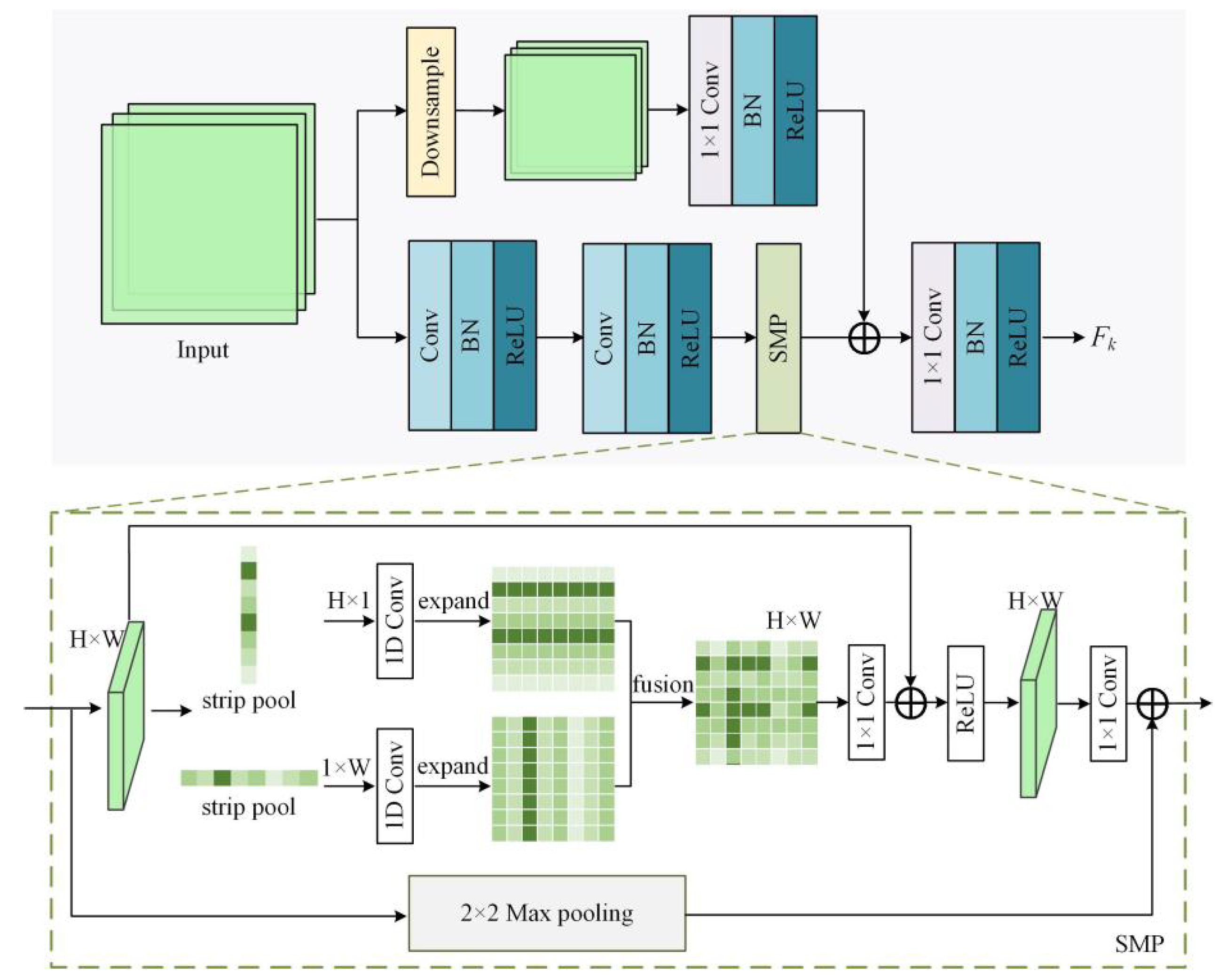
The MICM consists of four submodules, each of which has the same double-branch architecture (Figure 4). Taking X as an input, the lower branch extracts features δ k by using two convolution layers, each of which contains a batch normalization (BN) layer and a rectified linear unit (ReLU) activation function.
δ k = g ( δ k 1 ) , k = { 1 , 2 , 3 , 4 } ,
where g ( ) denotes the double convolution operations and δ k denotes the convolution feature of the k-th submodule when k = 1 ,   δ 0 = X . Then, the SMP is employed for feature abstraction and dimensionality reduction.
In this article, SMP is used to replace the max pooling operations of classical networks. Max pooling probes information within square windows, which limits the flexibility in capturing anisotropic context features. Strip pooling [45] resolves this problem well. The given convolution feature δ k is fed into a horizontal and vertical strip pooling layer simultaneously, resulting in two 1D features δ k h R C × H and δ k v R C × W :
δ k   i h = 1 W 0 j < W δ k ( i , j ) ,
δ k   j v = 1 H 0 i < H δ k ( i , j ) ,
Subsequently, δ k h and δ k v are converted into feature matrices with sizes of H × W via a 1D convolution. Then, the feature map δ k of the SMP structure in the k-th submodule is obtained by Equation (9):
δ k = MP ( δ k ) f s t = 2 ( ReLU ( δ k f s t = 1 ( δ k   i h + δ k   j v ) ) ) , k = { 1 , 2 , 3 , 4 } ,
where MP ( ) denotes a max pooling, f s t ( ) denotes a 1 × 1 convolution with a stride size of st, and represents the feature concatenation operation.
The upper branch downsamples the input and reshapes the feature dimensions to make them consistent with δ k . The resulting feature maps are connected with δ k , and subsequently a 1 × 1 convolution is utilized to acquire the subfeature Fk:
F k = f ( d s k ( F k 1 ) δ k ) , k = { 1 , 2 , 3 , 4 } ,
where F k denotes the intermediate feature of the k-th submodule when k = 1 ,   F 0 = X , d ( ) denotes the downsampling operation, s = { 1 2 , 1 4 , 1 8 , 1 16 } is the downsampling parameter, f ( ) denotes a 1 × 1 convolution, and represents the feature concatenation operation. The sizes of the four intermediate feature maps are {1282,642,322,162} pixels, and the numbers of channels are {128,256,512,1024}. Finally, the convolution feature FB with a size of 16 × 16 × 1024 is obtained via two convolution layers.

3.2.3. Decoder

The decoder takes the joint feature F, which concatenates the outputs of the TM and MICM, as the input for feature restoration (Figure 2). Two convolution layers are used to reshape the feature dimensions to 16 × 16 × 1024 . The resulting feature is restored to the same dimension as the input image by Equation (11):
γ k = ReLU ( BN ( TransposeConv ( γ k 1 ) ) ) , k = { 1 , 2 , 3 , 4 } ,
where γ k denotes the feature map of the k-th upsampling step, when k = 1 ,   γ 0 = F , and TransposeConv ( ) denotes the transposed convolution layer. Four skip connections [46] are adopted to combine the convolution features in the MICM with the upsampled feature maps. Such an operation effectively alleviates the loss of features over successive convolution and pooling operations.
γ ˜ k = ReLU ( BN ( Conv ( γ k δ k ) ) ) , k = { 1 , 2 , 3 , 4 } ,
where γ ˜ k denotes the feature map of the k-th double convolution, and the numbers of feature channels are {512,256,128,64}. Finally, the feature maps with 2 channels are acquired via a 1 × 1 convolution, and these maps are fed into the sigmoid layer to obtain the prediction result R.

3.3. Discriminator Network

An FCN-based discriminator network is designed; it contains a double-branch structure with different convolution kernel sizes. More information about different receptive fields can be obtained by multiscale inputs and convolution kernels with different sizes. The discriminator network receives the segmentation result R or ground-truth maps as input, as shown in part II of Figure 2. Features are extracted from the upper and lower branches (Equations (13) and (14)):
F k U = LeakyReLU ( Con v k e = 4 s t = 2 ( F k 1 U ) ) , k = { 1 , 2 , 3 , 4 } ,
F k D = LeakyReLU ( Con v k e = 2 s t = 2 ( d s ( R ) k 1 ) ) , k = { 2 , 3 , 4 } ,
where F k U and F k D denote the features obtained by the k-th convolution in the upper and lower branches, respectively. When k = 1, F 0 U = R , Con v k e s t ( ) represents a convolution with strides of st and kernel sizes of ke, LeakyReLU ( ) denotes the leaky ReLU activation function, and d s ( ) denotes the downsampling operation with a parameter s = 1 / 2 . The numbers of channels in the resulting four feature maps are {64,128,256,512}. Subsequently, the feature maps generated by the two branches are concatenated and fed into a 1 × 1 convolution and a classification layer. Last, the confidence map is acquired via a sigmoid operation, in which each pixel represents the approximation degree of the pixels in the segmented map with respect to the sample label. This map is utilized as a supervisory signal for unlabeled data.

3.4. Loss Function

The segmentation network and discriminator network are trained jointly via labeled samples. When inputting unlabeled samples, the discriminator network generates confidence maps to supervise the training of the segmentation network in a self-taught mechanism. The discriminator network is optimized by minimizing the binary cross-entropy loss L D :
L D = i , j ( ( 1 y ) log ( 1 O ( i , j ) R ) + y log O ( i , j ) Y ) , i H , j W ,
where O ( i , j ) R and O ( i , j ) Y represent confidence maps for the prediction maps R and ground-truth labels Y, respectively, (i, j) denotes pixel locations, and y represents the label of each pixel.
The multitask loss in [24] is optimized to train the segmentation network:
L S e g = L C E + λ a d v L a d v + λ s e m i L s e m i ,
where L C E , L a d v and L s e m i respectively indicate the cross-entropy loss, adversarial loss, and semi-supervised loss, and λ a d v and λ s e m i are weights utilized for adjusting L S e g . In this study, λ a d v is respectively set to 0.01 and 0.001 while using labeled and unlabeled samples. λ s e m i is equal to 0.1. Taking C as the number of categories, L C E is obtained by Equation (17):
L C E = i , j c C Y ( i , j , c ) log ( R ( i , j , c ) ) , i H , j W
The adversarial loss and semi-supervised loss are shown in Equations (18) and (19), respectively:
L a d v = i , j log O ( i , j ) R ,
L s e m i = i , j , c Y c u log R ( i , j , c ) u ,   if   O ( i , j ) τ 0 ,   otherwise ,
where R ( i , j , c ) u denotes the class c prediction results of the unlabeled data at location (i, j), Y c u denotes the pseudo-label of the class c of unlabeled data, O ( i , j ) represents the confidence map, and τ is a threshold value of 0.2.

4. Results

4.1. Datasets

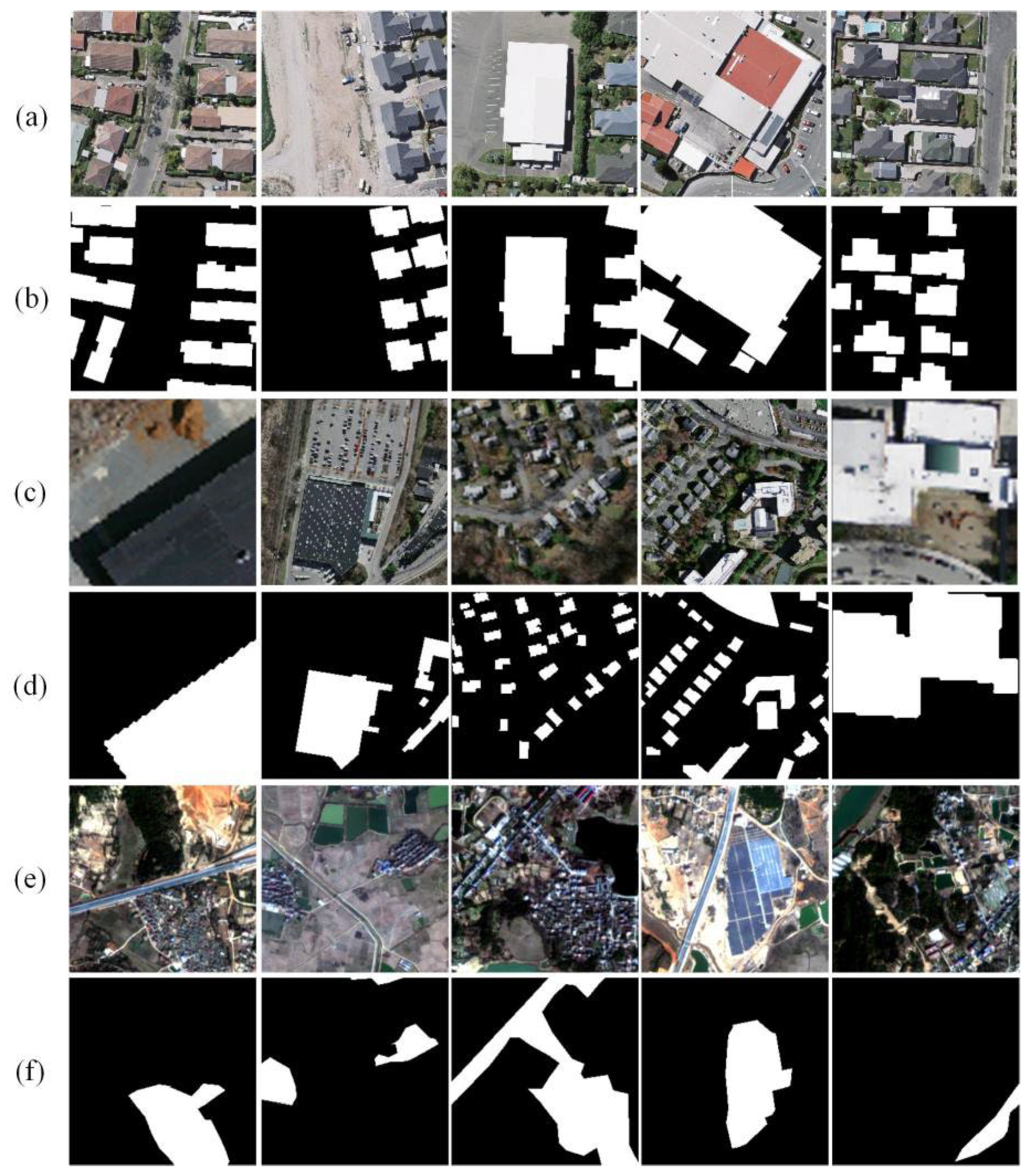
Three open-source remote sensing datasets with different spatial resolutions, including the WBD [35], MBD [36] and GID [10], were used for method verification. We clipped all images and labels into 256 × 256 image patches for model training and classification. Some building examples contained in the three datasets are shown in Figure 5. The labels were uniformly processed into binary images with a target value of 1 and a background value of 0.
  • WBD: This building dataset consists of 8189 aerial image tiles and contains 187,000 buildings with diverse usages, sizes and colors in Christchurch, New Zealand. The spatial resolution is 0.3 m. After cropping without overlap, 15,256 image patches were selected and randomly split into 14,256 patches for training and 1000 patches for testing.
  • MBD: The MBD is a large dataset for building segmentation that consists of 151 aerial images of the Boston area with 1500 × 1500 pixels. The spatial resolution is 1 m. A total of 11,384 image patches containing buildings with 256 × 256 pixels were chosen after cropping. These patches were further randomly divided into 10,384 patches for training and 1000 patches for testing.
  • GID: This land-use dataset contains 5 land-use categories and 150 Gaofen-2 satellite images, obtained from more than 60 different cities in China. The spatial resolution is 4 m. We extracted the building class and constructed a dataset containing 13,671 image patches for our experiments, among which 12,175 patches were used for training and 1496 were used for testing.

4.2. Experimental Procedure

4.2.1. Method Implementation

Several well-known semantic segmentation networks, i.e., DeepLabv2 [8], PSPNet [7], UNet [46], and TransUNet [44], with combinations of Transformer and convolution, were used for method comparisons under the SSAL framework. ResNet-101 was used as the backbone for DeepLabv2 and PSPNet. The numbers of Transformer layers and attention heads in TransUNet are set to 12 [44]. To validate the proposed method, we randomly sampled 1/8, 1/4 and 1/2 of images as labeled data and the remainder as unlabeled data. The quantities of labeled data are displayed in Table 1.
All models were implemented with Python 3.6 and PyTorch 1.2.0, which were powered by a 24-GB NVIDIA GeForce RTX 3090 GPU. The segmentation network was optimized using the stochastic gradient descent approach. The original learning rate was 2.5 × 10⁻⁴ and was declined via polynomial decay with a power of 0.9. The Adam optimizer [47], where the learning rate is 1 × 10⁻⁴, was utilized to optimize the discriminator network. All networks were trained over 80 K iterations and the batch size was 4. Adopting the same strategy used in [24], we started SSL after training 5000 iterations with labeled samples to avoid the model being influenced by the original noisy masks and predictions.

4.2.2. Method Evaluation Measures

Four assessment indices, precision, recall, F1 and mean intersection over union (mIoU), were utilized to evaluate the different methods. Equation (20) gives the definitions of these metrics:
Precision = T P T P + F P Recall = T P T P + F N F 1 = 2 × Precision × Recall Precision + Recall mIoU = 1 C c = 1 C T P T P + F P + F N ,
where TP indicates the quantity of building pixels correctly categorized, FP indicates the quantity of nonbuilding pixels categorized as buildings, FN indicates the quantity of building pixels incorrectly categorized as nonbuildings, and C is the quantity of categories. The F1 and mIoU metrics were utilized to comprehensively assess the model performance.

4.3. Experimental Results and Analysis

All the networks were trained on the WBD, MBD and GID using different quantities of labeled samples under the SSAL framework. The test sets did not participate in the model training and were used for evaluating and comparing the method performance.

4.3.1. Quantitative Analyses

Table 2, Table 3 and Table 4 show the building extraction accuracies achieved on the three datasets. In general, adding the quantity of labeled samples increases the accuracy measures of each approach. The F1 and mIoU measures of the proposed TRANet were the best on the three datasets, and this finding was consistent with the subsequent visualization analysis.
As shown in Table 2, the building extraction accuracies of all methods on the WBD were higher than 90%, except DeepLabv2 and PSPNet. PSPNet performed worst among all the models. When trained with fully labeled data, the four measures yielded by TRANet increased by 5.51%, 11.27%, 8.53% and 8.82%, compared with those of PSPNet. The UNet model performed the second best. With only 1/8 of the labeled data, UNet’s F1 and mIoU values were 92.88% and 91.82%, respectively, which were 0.5% lower than those of TRANet. The accuracy of TransUNet was slightly lower than that of UNet. The Transformer structure is added only at the top of the TransUNet encoder, resulting in limited global information. TRANet, which combines the Transformer and convolution, performed the best on the WBD.
Table 3 lists the accuracy measures produced by the different methods on the MBD. The accuracies of all models were lower than 80%. With 1/8 of the labeled data, the F1 and mIoU measures of TRANet were 72.21% and 74.54%, respectively, which were 5% lower than those obtained using fully labeled data. However, this method still performed the best. TRANet’s F1 and mIoU increased by approximately 0.82%~11.83% and 0.74%~7.5%, respectively, compared with those of other methods. The UNet model performed suboptimally. The F1 and mIoU measures of TransUNet were 3.19% and 2.24% lower than those of UNet, respectively, under 1/8 of the labeled data. The performances of DeepLabv2 and PSPNet were poor, and all the F1 and mIoU values were lower than 70%. The DeepLabv2 model performed slightly better than PSPNet.
On the GID, as shown in Table 4, TransUNet, using the Transformer structure, achieved better building extraction accuracy than UNet. When trained with 1/8 labeled samples, TransUNet’s F1 and mIoU values were 1.63% and 1.44% better than those of UNet, respectively. DeepLabv2 performed better than PSPNet and UNet. When trained with fully labeled data, DeepLabv2’s F1 and mIoU were 1.51% and 1.29% less than those of TRANet, respectively. TRANet performed the best. The four measures of TRANet, when training with 1/2 labeled data, decreased by 0.27%, 1.23%, 0.8%, and 0.68% relative to the metrics obtained when training with fully labeled data, where TRANet achieved an accuracy similar to that of using fully supervised training.

4.3.2. Qualitative Analyses

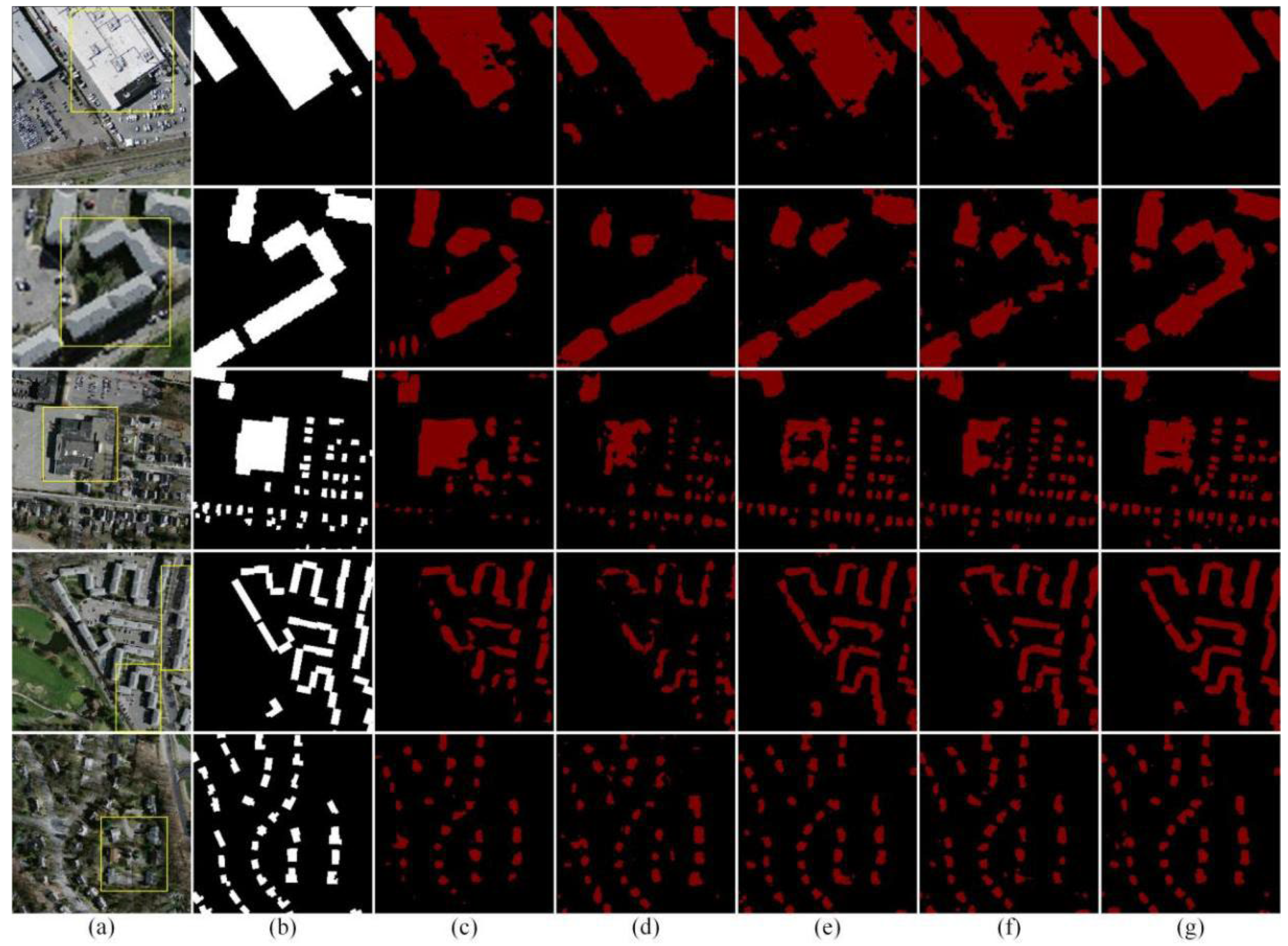
The semantic segmentation results obtained when training with 1/8 labeled samples under the SSAL framework were used for visual analysis. Figure 6, Figure 7 and Figure 8 show the representative building regions derived with the three datasets.
The WBD has high resolution and good image quality. Figure 6c,d show that the results obtained by DeepLabv2 and PSPNet exhibited many missed extractions and falsely extracted areas, and obvious distortions were present on the edges of buildings, especially in subregions 1 and 2. The extraction results of UNet and TransUNet had fewer missed extractions (subregions 1 and 2) and falsely extracted areas (subregion 4). TRANet extracted more complete building surfaces in subregions 2–5, and the details were closer to the reference labels.
The resolution of the MBD is 1 m. Many buildings with small areas are represented by only a few to more than a dozen pixels in the corresponding images; this situation brings difficulties to the fine extraction of buildings. As shown in Figure 7c,d, all results obtained by PSPNet and DeepLabv2 had large numbers of missed extractions, and the extracted buildings had irregular shapes and fuzzy boundaries. UNet extracted more complete small buildings with clear boundaries, as shown in Figure 7e, but obvious losses existed in the large buildings of subregion 3. In addition, the strip buildings in subregions 1, 2, and 4 were extracted incompletely. TRANet extracted complete buildings, especially in subregions 4 and 5 of Figure 7g, and the boundaries of small buildings and the surfaces of strip buildings demonstrated the better performance of this method, although small, missed extractions existed in subregions 2 and 3.
The GID has good image quality but relatively low resolution. Multiple complex objects, i.e., water bodies, roads, farmland, bare land, etc., are contained in one image. Buildings have irregular edges and are mostly distributed in pieces, which are easily mixed with other types of objects. Such a situation increases the difficulty of building extraction. Overall, all extraction results had missed extractions and falsely extracted areas. The falsely extracted areas in the results obtained by DeepLabv2, PSPNet, UNet and TransUNet were smaller, as shown in Figure 8c–f, but there were more missed extractions in subregions 2, 4 and 5. TRANet extracted more complete buildings than other models.
Based on the aforementioned quantitative and qualitative analyses, the proposed TRANet performed the best. TRANet uses the Transformer to obtain global contextual information and the MICM to extract local multiscale features simultaneously. The proposed SMP structure is designed to retain horizontal and vertical features, which alleviates the loss of details over continuous convolution operations. All these designs facilitate improvements in the building extraction accuracy.

5. Discussion

We performed four groups of ablation experiments to validate the performance of the designed double-branch segmentation network, the MICM, the SMP, and the discriminator network. The double-branch encoder is the core of TRANet, and it was verified by semi-supervised experiments with the WBD, MBD and GID under different amounts of labeled data, to fully illustrate the advantages of the Transformer combined with convolution. For the other three groups, 7128 labeled samples and 7128 unlabeled samples from the WBD were selected for the ablation experiments.

5.1. Comparison between Single/Double-Branch Encoder Structures

The encoder of the TRANet segmentation network contains a parallel TM and MICM, and it was verified via module replacement, along with the fixed decoder and discriminator network under the SSAL framework. Table 5 shows that the accuracies were low when the TM was used alone as the encoder, among which the F1 and mIoU were approximately 8.11~18.96% and 8.44~12.69% less than those obtained by the encoder using the MICM alone, respectively. The Transformer focuses on context modeling during the encoding phase and ignores the detailed localization of low-level features, which is hardly restored by upsampling. Convolution operations can extract rich low-level features. Combining the Transformer with convolution facilitates the improvement in the segmentation accuracy. The F1 and mIoU increased by approximately 0.13~19.44% and 0.14~13.09%, respectively, over the results obtained by using the single encoder. Therefore, TRANet utilizes the advantages of the Transformer and convolution to extract robust features, thereby improving semantic segmentation accuracy.

5.2. Comparison among Different Pooling Modules

The proposed SMP was verified by module replacement along with the fixed decoder and discriminator network under the SSAL framework. One set of experiments used a single-branch encoder, containing four simple “convolution-pooling” architectures, where the pooling layer was successively replaced by max pooling, strip pooling [45], and the SMP structure. These corresponding alternates were represented by CNN_MP, CNN_SP, and CNN_SMP. Another set of experiments used a double-branch encoder combining the TM and the aforementioned “convolution-pooling” architectures, which were represented by TM+CNN_MP, TM+CNN_SP, and TM+CNN_SMP. The achieved accuracy measures are listed in Table 6. The single- or double-branch encoders using the SMP performed the best when compared with those using other pooling structures, thereby proving the proposed SMP structure.

5.3. Comparison among Different Multiscale Modules

The MICM was verified by module replacement along with the fixed decoder and discriminator network under the SSAL framework. One set of experiments used a single-branch encoder, containing four simple “convolution-pooling” architectures and added atrous spatial pyramid pooling (ASPP) [8], selective kernel (SK) [48], and MICM modules to the encoder, which were represented by CNN, CNN+ASPP, CNN+SK, and CNN+MICM, respectively. Another set of experiments used the aforementioned double-branch encoder with different multiscale modules, which were represented by TM+CNN, TM+CNN+ASPP, TM+CNN+SK, and TM+CNN+MICM. Table 7 shows that the methods using multiscale modules achieved higher accuracy than those that did not utilize multiscale modules. Both the single- and double-branch encoders using the MICM performed better than those using other multiscale modules. The MICM captures multiscale input maps before feature extraction, which reduces the loss of details caused by continuous convolution operations with limited receptive fields.

5.4. Comparison among Different Discriminator Networks

The discriminator network in [24] and that proposed in this paper (represented by an additional *), along with five segmentation networks, including DeepLabv2, PSPNet, UNet, TransUNet and TRANet, were utilized for model training under the SSAL framework. Table 8 presents the achieved accuracy measures. The developed discriminator network facilitated the same segmentation network to obtain higher segmentation accuracy. This strategy was effective for all five segmentation networks. The proposed discriminator network can capture more information with different receptive fields by utilizing multiscale inputs and convolutions with different kernel sizes.

5.5. Model Parameter Discussions

Two important parameters in the TM of TRANet, the number of Transformer layers and number of heads, are represented by layer_num and head_num, respectively. We used 7128 labeled data and 7128 unlabeled data from the WBD for semi-supervised training, with different parameter settings, and analyzed the network performance. When the influence of layer_num was analyzed, head_num was fixed to 8, and layer_num was set to {4,8,12,16,20}. When the influence of head_num was analyzed, layer_num was fixed to 12, and head_num was set to {2,4,8,12,16}. Table 9 and Table 10 show that the highest accuracy was obtained when layer_num was 12 and head_num was 8. Therefore, this set of values was used in all experiments in this study.

6. Conclusions

In this article, we designed a novel semi-supervised adversarial semantic segmentation network for object extraction, from high-resolution remote sensing imagery, which leverages both the local feature extraction advantages of CNNs and the global context modeling abilities of the Transformer. Experimental results on three datasets with different spatial resolutions show that TRANet significantly increases the building extraction accuracies and makes the acquired segmentation results close to those obtained via fully supervised learning when a small number of labeled data are available. Future works will further fuse the multilevel features of the Transformer and CNNs to obtain more refined object information, thereby enhancing the performance of the segmentation network and applying it to segmentation tasks involving other objects in high-resolution remote sensing imagery.

Author Contributions

Conceptualization, Y.Z., M.W., X.Q., X.Z. and W.D.; methodology, Y.Z. and M.W.; validation, Y.Z. and M.Y.; formal analysis, Y.Z. and M.W.; data curation, Y.Z. and R.Y.; writing—original draft preparation, Y.Z.; writing—review and editing, Y.Z., M.Y. and M.W.; supervision, Y.Z. and M.W.; visualization, Y.Z.; funding acquisition, M.W. and Y.Z.; project administration, M.W. All authors have read and agreed to the published version of the manuscript.

Funding

This research was funded by the National Key R&D Program of China (grant number 2021YFB3901300), the National Natural Science Foundation of China (grant numbers 42071301, 41671341), the Jiangsu Province Water Conservancy Science and Technology Project (grant number 2021064), the Chongqing Agricultural Industry Digital Map Project (grant number 21C00346), and the Postgraduate Research and Practice Innovation Program of Jiangsu Province (KYCX21_1349).

Data Availability Statement

The data provided in this work are available from the corresponding authors.

Acknowledgments

We would like to sincerely thank the editors and reviewers for their time.

Conflicts of Interest

The authors declare no conflict of interest.

References

  1. Kang, J.; Wang, Z.; Zhu, R.; Sun, X.; Fernandez-Beltran, R.; Plaza, A. PiCoCo: Pixelwise Contrast and Consistency Learning for Semisupervised Building Footprint Segmentation. IEEE J. Sel. Top. Appl. Earth Obs. Remote Sens. 2021, 14, 10548–10559. [Google Scholar] [CrossRef]
  2. Su, Y.; Cheng, J.; Bai, H.; Liu, H.; He, C. Semantic Segmentation of Very-High-Resolution Remote Sensing Images via Deep Multi-Feature Learning. Remote Sens. 2022, 14, 533. [Google Scholar] [CrossRef]
  3. Long, J.; Shelhamer, E.; Darrell, T. Fully convolutional networks for semantic segmentation. IEEE Trans. Pattern Anal. Mach. Intell. 2015, 39, 640–651. [Google Scholar] [CrossRef]
  4. Alshehhi, R.; Marpu, P.R.; Woon, W.L.; Mura, M.D. Simultaneous extraction of roads and buildings in remote sensing imagery with convolutional neural networks. ISPRS J. Photogramm. Remote Sens. 2017, 130, 139–149. [Google Scholar] [CrossRef]
  5. Li, Y.; Lu, H.; Liu, Q.; Zhang, Y.; Liu, X. SSDBN: A Single-Side Dual-Branch Network with Encoder–Decoder for Building Extraction. Remote Sens. 2022, 14, 768. [Google Scholar] [CrossRef]
  6. Kang, J.; Guan, H.; Peng, D.; Chen, Z. Multi-scale context extractor network for water-body extraction from high-resolution optical remotely sensed images. Int. J. Appl. Earth Obs. Geoinf. 2021, 103, 102499. [Google Scholar] [CrossRef]
  7. Zhao, H.; Shi, J.; Qi, X.; Wang, X.; Jia, J. Pyramid scene parsing network. In Proceedings of the IEEE Conference on Computer Vision and Pattern Recognition, Honolulu, HI, USA, 21–26 July 2017; pp. 6230–6239. [Google Scholar] [CrossRef] [Green Version]
  8. Chen, L.C.; Papandreou, G.; Kokkinos, I.; Murphy, K.; Yuille, A.L. DeepLab: Semantic image segmentation with deep convolutional nets, atrous convolution, and fully connected CRFs. IEEE Trans. Pattern Anal. Mach. Intell. 2018, 40, 834–848. [Google Scholar] [CrossRef] [Green Version]
  9. Fu, J.; Liu, J.; Tian, H.; Li, Y.; Bao, Y.; Fang, Z.; Lu, H. Dual Attention Network for Scene Segmentation. In Proceedings of the IEEE Conference on Computer Vision and Pattern Recognition, Long Beach, NY, USA, 15–20 June 2019; pp. 3141–3149. [Google Scholar] [CrossRef] [Green Version]
  10. Tong, X.; Xia, G.; Lu, Q.; Shen, H.; Li, S.; You, S.; Zhang, L. Land-Cover Classification with High-Resolution Remote Sensing Images Using Transferable Deep Models. arXiv 2019, arXiv:1807.05713. Available online: https://arxiv.org/abs/1807.05713 (accessed on 20 November 2019). [CrossRef] [Green Version]
  11. Zhang, M.; Hu, X.; Zhao, L.; Lv, Y.; Luo, M. Learning dual multi-scale manifold ranking for semantic segmentation of high-resolution images. Remote Sens. 2017, 9, 500. [Google Scholar] [CrossRef] [Green Version]
  12. Gerke, M.; Rottensteiner, F.; Wegner, J.D.; Sohn, G. ISPRS Semantic Labeling Contest. 2014. Available online: https://www.isprs.org/education/benchmarks/UrbanSemLab/2d-sem-label-potsdam.aspx (accessed on 7 September 2014).
  13. Kemker, R.; Luu, R.; Kanan, C. Low-shot learning for the semantic segmentation of remote sensing imagery. IEEE Trans. Geosci. Remote Sens. 2018, 56, 6214–6223. [Google Scholar] [CrossRef] [Green Version]
  14. Wambugu, N.; Chen, Y.; Xiao, Z.; Tan, K.; Wei, M.; Liu, X.; Li, J. Hyperspectral image classification on insufficient-sample and feature learning using deep neural networks: A review. Int. J. Appl. Earth Obs. Geoinf. 2021, 105, 102603. [Google Scholar] [CrossRef]
  15. Lee, D.H. Pseudo-Label: The Simple and Efficient Semi-Supervised Learning Method for Deep Neural Networks. In Proceedings of the 30th International Conference on Machine Learning, Atlanta, GA, USA, 16–21 June 2013. [Google Scholar]
  16. Qiao, S.; Shen, W.; Zhang, Z.; Wang, B.; Yuille, A. Deep Co-Training for Semi-Supervised Image Recognition. In Proceedings of the 15th European Conference on Computer Vision, Munich, Germany, 8–14 September 2018; pp. 142–159. [Google Scholar] [CrossRef] [Green Version]
  17. Laine, S.; Aila, T. Temporal ensembling for semisupervised learning. arXiv 2017, arXiv:1610.02242. Available online: https://arxiv.org/abs/1610.02242 (accessed on 15 March 2017).
  18. Tarvainen, A.; Valpola, H. Mean teachers are better role models: Weight-averaged consistency targets improve semisupervised deep learning results. arXiv 2017, arXiv:1703.01780. Available online: https://arxiv.org/abs/1703.01780 (accessed on 6 March 2017).
  19. Berthelot, D.; Carlini, N.; Goodfellow, I.; Oliver, A.; Papernot, N.; Raffel, C. MixMatch: A holistic approach to semi-supervised learning. arXiv 2019, arXiv:1905.02249. Available online: https://arxiv.org/abs/1905.02249 (accessed on 23 October 2019).
  20. Sohn, K.; Berthelot, D.; Li, C.; Zhang, Z.; Carlini, N.; Cubuk, E.D.; Kurakin, A.; Zhang, H.; Raffel, C. FixMatch: Simplifying semi-supervised learning with consistency and confidence. arXiv 2020, arXiv:2001.07685v2. Available online: https://arxiv.org/abs/2001.07685v2 (accessed on 25 November 2020).
  21. Odena, A. Semi-supervised learning with generative adversarial networks. arXiv 2016, arXiv:1606.01583. [Google Scholar]
  22. Wang, L.; Sun, Y.; Wang, Z. CCS-GAN: A semi-supervised generative adversarial network for image classification. Vis. Comput. 2021, 4, 1–13. [Google Scholar] [CrossRef]
  23. Luc, P.; Couprie, C.; Chintala, S.; Verbeek, J. Semantic segmentation using adversarial networks. arXiv 2016, arXiv:1611.08408. Available online: https://arxiv.org/abs/1611.08408 (accessed on 25 November 2016).
  24. Hung, W.C.; Tsai, Y.H.; Liou, Y.T.; Lin, Y.Y.; Yang, M.H. Adversarial learning for semi-supervised semantic segmentation. arXiv 2018, arXiv:1802.07934. Available online: https://arxiv.org/abs/1802.07934 (accessed on 24 July 2018).
  25. Goodfellow, I.J.; Pouget-Abadie, J.; Mirza, M.; Xu, B.; Warde-Farley, D.; Ozair, S.; Courville, A.; Bengio, Y. Generative adversarial networks. arXiv 2014, arXiv:1406.2661. [Google Scholar] [CrossRef]
  26. Zheng, S.; Lu, J.; Zhao, H.; Zhu, X.; Zhang, L. Rethinking semantic segmentation from a sequence-to-sequence perspective with transformers. arXiv 2020, arXiv:2012.15840. Available online: https://arxiv.org/abs/2012.15840 (accessed on 31 December 2020).
  27. Chen, Z.; Wang, C.; Li, J.; Fan, W.; Du, J.; Zhong, B. Adaboost-like End-to-End multiple lightweight U-nets for road extraction from optical remote sensing images. Int. J. Appl. Earth Obs. Geoinf. 2021, 100, 2341. [Google Scholar] [CrossRef]
  28. Hu, J.; Shen, L.; Albanie, S.; Sun, G.; Wu, E. Squeeze-and-excitation networks. IEEE Trans. Pattern Anal. Mach. Intell. 2020, 42, 2011–2023. [Google Scholar] [CrossRef] [PubMed] [Green Version]
  29. Dosovitskiy, A.; Beyer, L.; Kolesnikov, A.; Weissenborn, D.; Zhai, X.; Unterthiner, T.; Dehghani, M.; Minderer, M.; Heigold, G.; Gelly, S.; et al. An image is worth 16 × 16 words: Transformers for image recognition at scale. arXiv 2020, arXiv:2010.11929. [Google Scholar] [CrossRef]
  30. Liu, Z.; Lin, Y.; Cao, Y.; Hu, H.; Wei, Y.; Zhang, Z.; Lin, S.; Guo, B. Swin Transformer: Hierarchical vision transformer using shifted windows. arXiv 2021, arXiv:2103.14030. [Google Scholar] [CrossRef]
  31. Yang, F.; Yang, H.; Fu, J.; Lu, H.; Guo, B. Learning texture transformer network for image super-resolution. In Proceedings of the Conference on Computer Vision and Pattern Recognition, Seattle, DC, USA, 13–19 June 2020; pp. 5790–5799. [Google Scholar] [CrossRef]
  32. Wang, Z.; Zhao, J.; Zhang, R.; Li, Z.; Lin, Q.; Wang, X. UATNet: U-Shape Attention-Based Transformer Net for Meteorological Satellite Cloud Recognition. Remote Sens. 2022, 14, 104. [Google Scholar] [CrossRef]
  33. Vaswani, A.; Shazeer, N.; Parmar, N.; Uszkoreit, J.; Jones, L.; Gomez, A.N.; Kaiser, L.; Polosukhin, I. Attention is All you Need. In Proceedings of the 31st Conference on Neural Information Processing Systems, Long Beach, NY, USA, 4–9 December 2017; pp. 6000–6010. [Google Scholar] [CrossRef]
  34. Zhang, Y.; Liu, H.; Hu, Q. TransFuse: Fusing transformers and cnns for medical image segmentation. arXiv 2021, arXiv:2102.08005. [Google Scholar] [CrossRef]
  35. Ji, S.; Wei, S.; Lu, M. Fully convolutional networks for multi-source building extraction from an open aerial and satellite imagery dataset. IEEE Trans. Geosci. Remote Sens. 2019, 57, 574–586. [Google Scholar] [CrossRef]
  36. Mnih, V. Machine Learning for Aerial Image Labeling. Ph.D. Dissertation, Department Computer Science, Toronto University, Toronto, ON, Canada, 2013. [Google Scholar]
  37. Mittal, S.; Tatarchenko, M.; Brox, T. Semi-supervised semantic segmentation with high- and low-level consistency. IEEE Trans. Pattern Anal. Mach. Intell. 2021, 43, 1369–1379. [Google Scholar] [CrossRef] [Green Version]
  38. He, Y.; Wang, J.; Liao, C.; Shan, B.; Zhou, X. ClassHyPer: ClassMix-Based Hybrid Perturbations for Deep Semi-Supervised Semantic Segmentation of Remote Sensing Imagery. Remote Sens. 2022, 14, 879. [Google Scholar] [CrossRef]
  39. Souly, N.; Spampinato, C.; Shah, M. Semi Supervised Semantic Segmentation Using Generative Adversarial Network. In Proceedings of the IEEE International Conference on Computer Vision, Venice, Italy, 22–29 October 2017; pp. 5689–5697. [Google Scholar] [CrossRef]
  40. Zhang, J.; Li, Z.; Zhang, C.; Ma, H. Robust Adversarial Learning for Semi-Supervised Semantic Segmentation. In Proceedings of the IEEE International Conference on Image Processing, Abu Dhabi, United Arab Emirates, 25–28 October 2020; pp. 728–732. [Google Scholar] [CrossRef]
  41. Sun, X.; Shi, A.; Huang, H.; Mayer, H. BAS4Net: Boundary-aware semi-supervised semantic segmentation network for very high resolution remote sensing images. IEEE J. Sel. Top. Appl. Earth Obs. Remote Sens. 2020, 13, 5398–5413. [Google Scholar] [CrossRef]
  42. Luo, H.; Chen, C.; Fang, L.; Zhu, X.; Lu, L. High-resolution aerial images semantic segmentation using deep fully convolutional network with channel attention mechanism. IEEE J. Sel. Top. Appl. Earth Obs. Remote Sens. 2019, 12, 3492–3507. [Google Scholar] [CrossRef]
  43. Huang, J.; Zhang, X.; Sun, Y.; Xin, Q. Attention-guided label refinement network for semantic segmentation of very high resolution aerial orthoimages. IEEE J. Sel. Top. Appl. Earth Obs. Remote Sens. 2021, 14, 4490–4503. [Google Scholar] [CrossRef]
  44. Chen, J.; Lu, Y.; Yu, Q.; Luo, X.; Adeli, E.; Wang, Y.; Lu, L.; Yuille, L.A.; Zhou, Y. TransUNet: Transformers make strong encoders for medical image segmentation. arXiv 2021, arXiv:2102.04306. [Google Scholar]
  45. Hou, Q.; Zhang, L.; Cheng, M.; Feng, J. Strip Pooling: Rethinking Spatial Pooling for Scene Parsing. In Proceedings of the IEEE Conference on Computer Vision and Pattern Recognition, Seattle, WA, USA, 13–19 June 2020; pp. 4002–4011. [Google Scholar] [CrossRef]
  46. Ronneberger, O.; Fischer, P.; Brox, T. U-Net: Convolutional Networks for Biomedical Image Segmentation. In Proceedings of the Medical Image Computing and Computer Assisted Intervention, Munich, Germany, 5–9 October 2015; pp. 234–241. [Google Scholar] [CrossRef] [Green Version]
  47. Kingma, D.; Ba, J. Adam: A method for stochastic optimization. arXiv 2014, arXiv:1412.6980. Available online: https://arxiv.org/abs/1412.6980 (accessed on 22 December 2014).
  48. Li, X.; Wang, W.; Hu, X.; Yang, J. Selective Kernel Networks. In Proceedings of the IEEE Conference on Computer Vision and Pattern Recognition, Long Beach, NY, USA, 15–20 June 2019; pp. 510–519. [Google Scholar] [CrossRef] [Green Version]
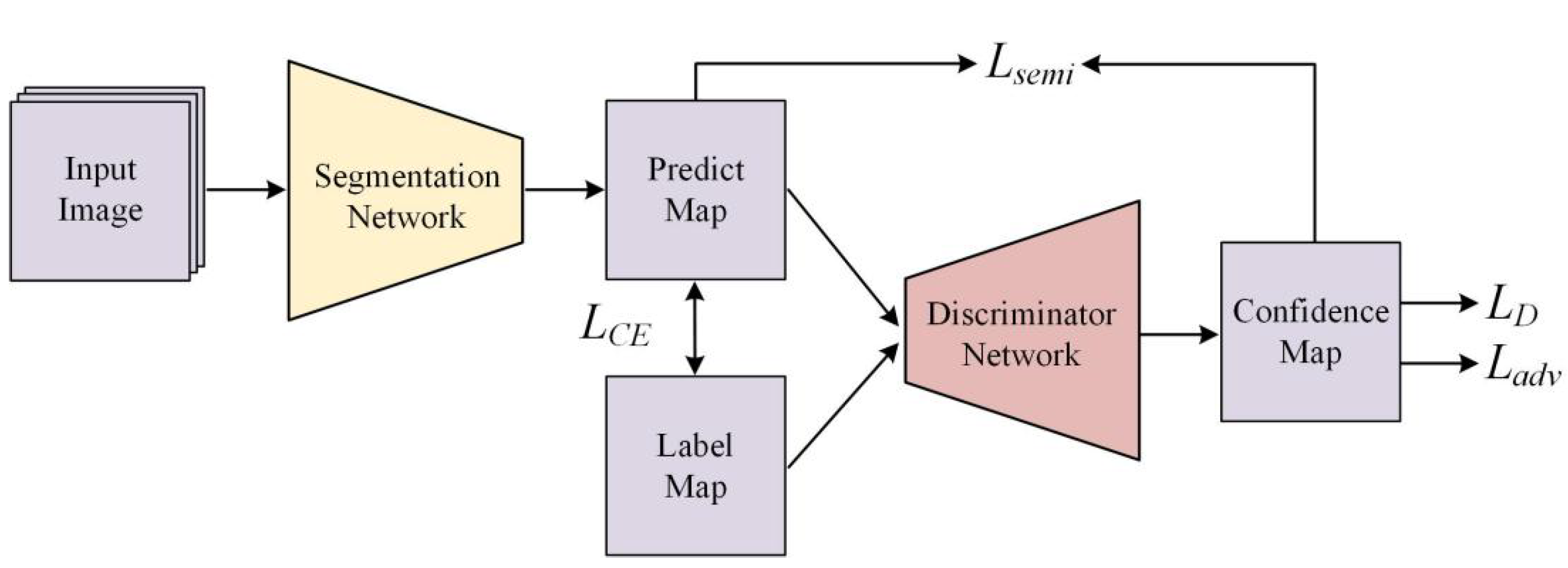
Figure 1. A typical SSAL framework, where L C E , L D , L a d v and L s e m i respectively represent cross-entropy loss, discriminator loss, adversarial loss, and semi-supervised loss, respectively.
Remotesensing 14 01786 g001
Figure 2. Architecture of TRANet.
Remotesensing 14 01786 g002
Figure 3. Transformer module.
Remotesensing 14 01786 g003
Figure 4. The MICM submodule and SMP architecture.
Remotesensing 14 01786 g004
Figure 5. Different buildings in the three datasets: (a,b) are WBD building images and corresponding labels, (c,d) are MBD building images and corresponding labels, and (e,f) are GID building images and corresponding labels, respectively.
Remotesensing 14 01786 g005
Figure 6. Typical building extraction results on the WBD. (a) Images. (b) Labels. (c) DeepLabv2. (d) PSPNet. (e) UNet. (f) TransUNet. (g) TRANet. Yellow boxes identify partial differences between the different methods.
Remotesensing 14 01786 g006
Figure 7. Typical building extraction results on the MBD. (a) Images. (b) Labels. (c) DeepLabv2. (d) PSPNet. (e) UNet. (f) TransUNet. (g) TRANet. Yellow boxes identify partial differences between the different methods.
Remotesensing 14 01786 g007
Figure 8. Typical building extraction results on the GID. (a) Images. (b) Labels. (c) DeepLabv2. (d) PSPNet. (e) UNet. (f) TransUNet. (g) TRANet. Yellow boxes identify partial differences between the different methods.
Remotesensing 14 01786 g008
Table 1. Amounts of labeled data.
DatasetsLabeled Data Amount
1/81/41/2Full
WBD17823564712814,256
MBD12982596519210,384
GID15223044608812,671
Table 2. Building extraction accuracies obtained with different quantities of labeled data on the WBD. The highest accuracy is displayed in bold.
MethodLabeled Data Amount
1/81/4
RecallPrecisionF1mIoURecallPrecisionF1mIoU
DeepLabv20.89650.87130.88370.87140.91870.85860.88760.8759
PSPNet0.88340.82670.85410.84290.88860.83010.85830.8470
UNet0.92930.92840.92880.91820.94210.93520.93870.9290
TransUNet0.91930.92020.91970.90840.93620.92820.93220.9219
TRANet0.93640.93010.93320.92300.94950.93460.94200.9327
Method1/2Full
RecallPrecisionF1mIoURecallPrecisionF1mIoU
DeepLabv20.89730.89240.89490.88240.92040.88310.90130.8895
PSPNet0.90020.82200.85930.84830.90200.82940.86420.8529
UNet0.95120.93940.94530.93640.95540.94080.94800.9394
TransUNet0.94570.93170.9387 0.9290 0.94960.93370.94160.9323
TRANet0.95470.94020.94740.93870.95710.94210.94950.9411
Table 3. Building extraction accuracies obtained with different quantities of labeled data on the MBD. The highest accuracy is displayed in bold.
MethodLabeled Data Amount
1/81/4
RecallPrecisionF1mIoURecallPrecisionF1mIoU
DeepLabv20.77060.49640.60380.67040.70320.57990.63560.6856
PSPNet0.72960.52240.60880.67140.75760.49230.59680.6659
UNet0.74900.68190.71390.73800.77520.69430.73250.7523
TransUNet0.72520.64370.68200.71560.76300.68520.72200.7443
TRANet0.78390.66930.72210.74540.77850.71780.74690.7627
Method1/2Full
RecallPrecisionF1mIoURecallPrecisionF1mIoU
DeepLabv20.73980.55260.63260.68580.72920.63120.67660.7124
PSPNet0.75900.50620.60730.67200.76230.50600.60830.6726
UNet0.79880.72250.75880.77230.81270.74020.77480.7848
TransUNet0.79260.70010.74350.76080.80470.71800.75890.7726
TRANet 0.7987 0.73550.76580.77750.81600.74820.78060.7894
Table 4. Building extraction accuracies obtained with different quantities of labeled data on the GID. The highest accuracy is displayed in bold.
MethodLabeled Data Amount
1/81/4
RecallPrecisionF1mIoURecallPrecisionF1mIoU
DeepLabv20.85600.69460.76690.76790.82810.73810.78050.7773
PSPNet0.80030.65530.72050.73020.80640.67010.73200.7388
UNet0.76470.74600.75520.75350.77310.74420.75830.7565
TransUNet0.79040.75340.77150.76790.75380.77110.76240.7582
TRANet0.76590.79390.77970.77280.77650.80520.79050.7823
Method1/2Full
RecallPrecisionF1mIoURecallPrecisionF1mIoU
DeepLabv20.82880.75330.78930.78440.83580.75070.79100.7862
PSPNet0.78500.71220.74680.74860.82680.68510.74930.7530
UNet0.81540.73260.77180.76970.83260.75320.79090.7860
TransUNet0.83680.75190.79210.78720.82400.76870.79540.7892
TRANet0.84060.75970.79810.79230.84330.77200.80610.7991
Table 5. Building extraction accuracies with single/double-branch encoders. The highest accuracy is displayed in bold.
DatasetEncoderLabeled Data Amount
1/81/41/2
RecallPrecisionF1mIoURecallPrecisionF1mIoURecallPrecisionF1mIoU
WBDTM0.82580.82050.82310.81250.85990.84650.85320.84110.88010.85050.8650 0.8529
MICM0.93550.92930.93240.92210.93640.93960.93800.92820.95620.93610.94610.9373
TM+MICM0.93640.93010.93320.92300.94950.93460.94200.93270.95470.94020.94740.9387
MBDTM0.54610.51870.53210.61690.61610.48590.54330.62910.65790.5050 0.57140.6466
MICM0.74770.66880.7060 0.73270.7809 0.7103 0.74390.76070.78920.73480.7610.7735
TM+MICM0.78390.66930.72210.74540.77850.71780.74690.76270.79870.73550.76580.7775
GIDTM0.72280.58780.64830.67620.75340.6269 0.68430.70190.7630 0.62990.69010.7065
MICM0.75840.77340.7658 0.76130.78150.77020.77580.77080.80390.77870.79110.7846
TM+MICM0.76590.79390.77970.77280.7765 0.80520.79050.78230.84060.75970.79810.7923
Table 6. Accuracy assessment of TRANet in terms of building extraction with different pooling modules. The highest accuracy is displayed in bold.
MethodRecallPrecisionF1mIoU
CNN_MP0.94760.93600.94180.9325
CNN_SP0.95020.93460.94240.9332
CNN_SMP0.95320.93910.94610.9373
TM+CNN_MP0.9518 0.93980.94580.9369
TM+CNN_SP0.94530.93660.94090.9315
TM+CNN_SMP0.95470.94020.94740.9387
Table 7. Building extraction accuracies with different multiscale modules. The highest accuracy is displayed in bold.
MethodRecallPrecisionF1mIoU
CNN0.94760.9360 0.94180.9325
CNN+ASPP0.95150.93570.94350.9344
CNN+SK0.95460.93790.94620.9374
CNN+MICM0.95590.93790.94680.9381
TM+CNN0.95180.93980.94580.9369
TM+CNN+ASPP0.95400.93770.94580.9370
TM+CNN+SK0.95390.93910.94640.9377
TM+CNN+MICM0.95470.94020.94740.9387
Table 8. Building extraction accuracies with different discriminator networks. The highest accuracy is displayed in bold.
MethodRecallPrecisionF1mIoUMethodRecallPrecisionF1mIoU
DeepLabv20.90420.85640.87970.8677DeepLabv2 *0.89730.89240.89490.8824
PSPNet0.87380.82830.85040.8391PSPNet *0.90020.82200.85930.8483
UNet0.94150.93290.93720.9274UNet *0.95120.93940.94530.9364
TransUNet0.94510.93020.93760.9279TransUNet *0.94570.93170.93870.9290
TRANet0.95040.93860.94450.9354TRANet *0.95470.94020.94740.9387
Table 9. Building extraction accuracies under different layer_num settings when head_num = 8. The highest accuracy is displayed in bold.
layer_numRecallPrecisionF1mIoU
40.94770.92360.93550.9257
80.95020.92820.93910.9296
120.95470.94020.94740.9387
160.94430.93610.94020.9307
200.94530.92780.93650.9267
Table 10. Building extraction accuracies under different head_num settings when layer_num = 12. The highest accuracy is displayed in bold.
head_numRecallPrecisionF1mIoU
20.94610.93360.93980.9303
40.94670.93470.94070.9313
80.95470.94020.94740.9387
120.94560.93270.93910.9295
160.93280.94070.93670.9268
Publisher’s Note: MDPI stays neutral with regard to jurisdictional claims in published maps and institutional affiliations.