Article

Optimal Band Selection for Airborne Hyperspectral Imagery to Retrieve a Wide Range of Cyanobacterial Pigment Concentration Using a Data-Driven Approach

1
Graduate School of Civil, Environmental and Plant Engineering, Konkuk University, Seoul 05029, Korea
2
Division of Civil and Environmental and Plant Engineering, Konkuk University, Seoul 05029, Korea
3
Center for Environmental Data Strategy, Korea Environment Institute, Sejong 30147, Korea
4
Water Quality Assessment Research Division, National Institute of Environmental Research, Incheon 22689, Korea
5
School of Urban and Environmental Engineering, Ulsan National Institute of Science and Technology, Ulsan 44919, Korea
6
Office for Busan Region Management of the Nakdong River, Korea Water Resources Corporation (K-Water), Busan 49300, Korea
*
Author to whom correspondence should be addressed.
Remote Sens. 2022, 14(7), 1754; https://doi.org/10.3390/rs14071754
Submission received: 23 February 2022 / Revised: 29 March 2022 / Accepted: 4 April 2022 / Published: 6 April 2022
(This article belongs to the Special Issue Optical Remote Sensing for Surface Water Parameters Retrieval)

Abstract

:
Understanding the concentration and distribution of cyanobacteria blooms is an important aspect of managing water quality problems and protecting aquatic ecosystems. Airborne hyperspectral imagery (HSI)—which has high temporal, spatial, and spectral resolutions—is widely used to remotely sense cyanobacteria bloom, and it provides the distribution of the bloom over a wide area. In this study, we determined the input spectral bands that were relevant in effectively estimating the main two pigments (PC, Phycocyanin; Chl-a, Chlorophyll-a) of cyanobacteria by applying data-driven algorithms to HSI and then evaluating the change in the spatio-temporal distribution of cyanobacteria. The input variables for the algorithms consisted of reflectance band ratios associated with the optical properties of PC and Chl-a, which were calculated by the selected hyperspectral bands using a feature selection method. The selected input variable was composed of six reflectance bands (465.7–589.6, 603.6–631.8, 641.2–655.35, 664.8–679.0, 698.0–712.3, and 731.4–784.1 nm). The artificial neural network showed the best results for the estimation of the two pigments with average coefficients of determination 0.80 and 0.74. This study proposes relevant input spectral information and an algorithm that can effectively detect the occurrence of cyanobacteria in the weir pool along the Geum river, South Korea. The algorithm is expected to help establish a preemptive response to the formation of cyanobacterial blooms, and to contribute to the preparation of suitable water quality management plans for freshwater environments.

Graphical Abstract

1. Introduction

Cyanobacterial blooms, also named algal blooms, are massive growths of cyanobacteria in eutrophic lakes or rivers with low flow rates which change the color of the water surface to green. Recently, the duration, intensity, and frequency of algal blooms have gradually been increasing due to global warming, urbanization, and changes in precipitation patterns [1]. Excessive occurrence of algae poses environmental, societal, and economic threats due to the resulting damage to the aquatic ecosystems and the health of the aquatic animals and plants therein, as well as increased water purification costs due to harmful algal blooms (HABs)-associated toxins [2,3]. Understanding the patterns of distribution of algal blooms is very important for reducing the negative effects of the blooms on aquatic environments [4]. The study area, Baekje weir (BJW) pool along the Geum river, South Korea, has problems due to the periodic occurrence of algal blooms and is in need of improved monitoring and management tools.
Conventional water quality monitoring in rivers and lakes is implemented at a specific time and location to measure concentrations. Single-point sampling methods are limited in their ability to identify the spatial and temporal distributions of HABs. Fixed sensors have also been widely used as real-time and automatic systems for monitoring HABs. In situ sensor networks are limited in terms of their spatial and temporal resolutions and reliability, which is due to the maintenance problem involving the water quality observation sensor. To address these monitoring issues, many researchers have applied remote sensing techniques. Remote sensing can achieve regular-interval monitoring and detection of a wide area by measuring the reflectance or emission of objects.
Various types of multispectral and hyperspectral imagery have been used to remotely detect harmful algal blooms in coastal and inland waters [5,6,7,8,9]. In particular, hyperspectral imageries provide fine spectral data, thereby leading us to investigate the detailed statistical relations. Many empirical models, such as a band ratio algorithm that considers the relationship between spectral reflectance and algal pigments, were constructed to estimate algal pigments using spectral reflectance from remotely sensed data [10]. The band ratios in these models have typically been calculated using a small number of bands (less than four bands, e.g., 443, 665, 704, and 740 nm) due to the limited number of reflectance bands available from 400 nm to 900 nm. Eight different bands from satellite data were applied to machine learning models to estimate Chlorophyll-a (Chl-a) in coastal water [11,12]. A few of these studies have used airborne hyperspectral imagery with a fine spectral resolution (4 to 7 nm). Kutser et al. [13] used AISA hyperspectral spectrometer to obtain fine spectral data (7 nm resolution), but they applied an inverse model using a specific spectral band data to estimate Chl-a. Lunetta et al. [14] and Li et al. [15] retrieved Chl-a using a band ratio algorithm based on 673, 675, 693, and 704 nm, which were values obtained from AVIRIS and AISA hyperspectral imagery. Pyo et al. [16,17] obtained 86 reflectance bands from 400 to 800 nm taken by the AISA eagle sensor (4–5 nm resolution) and they applied all band data to construct machine learning models to estimate Chl-a and phycocyanin (PC) in a reservoir. Keller et al. [18] used 111 spectral bands from the hyperspectral snapshot sensor Cubert UHD 285, and the band data was used to develop linear and nonlinear bio-optical models for Chl-a in a river. Airborne hyperspectral imagery may provide fine spectral data, which can be used to investigate the statistical relations in detail. However, the existing literature studies have rarely evaluated the statistical relationships between fine-resolution spectral reflectance and each algal pigment. Some studies have used conventional spectral reflectance data to construct band ratio algorithms based on a small number of bands even though they observed fine-resolution hyperspectral [13,14,15]. Some studies have applied numerous spectral reflectance (more than 86 bands) data to a machine learning model [16,17,18]. Applying numerous reflectance bands may lead to increases in complexity, uncertainty, and input noise in the model and cause overfitting, low accuracy, and difficult interpretation [19]. That is, there have been few studies examining relevant feature selection for inputs of empirical models among fine-resolution hyperspectral data.
Therefore, to construct accurate and reliable empirical models, it is important to select relevant input reflectance bands. PC estimation mainly uses the wavelengths from 600 to 625 nm and from 700 to 720 nm in fresh water, and the 625 to 650 nm wavelength is used in some cases as well [20,21,22]. In the case of Chl-a, the wavelength range from 670 to 700 nm was used [23,24]. In general, the reflectivity of the eutrophic water surface shows low reflectance at 600 to 620 nm and 670 to 675 nm, and reflectance at around 650 nm. It also shows a peak at 700 to 724 nm, which is attributed to the strong absorption and fluorescence of PC and Chl-a [25,26]. The spectral wavelengths used to estimate PC or Chl-a vary according to the sites and concentration levels. In a high Chl-a concentration condition, the peak at 550 to 580 nm is slightly shifted to higher wavelengths, and the magnitude of the peak near 700 nm is significantly higher than it is for the low condition. Moreover, the magnitude of peaks is shifted depending on the spatial distribution of cyanobacterial density [25,27].
Therefore, the objectives of this study are to (a) determine relevant spectral bands within the range of 400–800 nm for use in empirical algorithms to effectively retrieve two pigments, (b) apply the selected input spectral reflectance data to empirical algorithms such as data-driven models, (c) evaluate the performance of the algorithms, and (d) suggest the best input spectral band combination and an algorithm that shows good performance for understanding the characteristics of the spatial distribution in a weir pool.

2. Materials and Methods

2.1. Study Area

BJW in South Korea was constructed in October 2011 to secure water storage in Geum river and reduce flood and drought damage (Figure 1). The weir is located 60 km upstream from the river estuary, and the basin area of the weir is 7976 km2 while its width and height are 311 m (movable 120 m, fixed 191 m), and 5.5 m, respectively. The manageable water level and storage capacity of water are 4.2 m and 24.2 × 10⁶ m3, respectively. Since the construction of the weir, cyanobacteria blooms have become a major concern due to continued drought, increases in water temperature, accumulation of nutrients load, and increased residence time. The algae alert based on an increase in the density of cyanobacteria has been steadily issued from 2012 to 2018.

2.2. Data Acquisition

A total of nine monitoring events were conducted to collect water samples, field hyperspectral reflectance, and airborne hyperspectral imagery during the 2-year period from 2016 to 2017 in the BJW (Figure 1 and Table 1). Water sampling and field hyperspectral measurement were performed concurrently with image acquisition by an aircraft equipped hyperspectral sensor. Water samples were analyzed for PC, Chl-a, and suspended solid.

2.2.1. Hyperspectral Imagery

Hyperspectral sensors measure reflectivity over hundreds of spectral bands for inland water. The high spectral resolution data of water surface reflectance are ideal data for the development and validation of PC algorithms [28,29]. The hyperspectral image sensor (AISA Eagle, SPECIM Inc., Oulu, Finland) has a spectral range of 400 to 970 nm, and a (4–5) nm spectral resolution. The spatial resolution of the hyperspectral imageries taken from the aircraft is 2 m, and the average river width in the 23 km upstream, where the observation was conducted, is 310 m (150 cells). Field hyperspectral reflectance data were collected using hand-held spectroradiometer (FieldSpec HandHeld2, ASD, Inc., Longmont, CO, USA). Field hyperspectral reflectance includes water surface reflectance, sky radiance, and irradiance [30]. Geometry correction and atmospheric correction using field hyperspectral data and MODTRAN 6 software were performed to improve the surface reflectance of the captured hyperspectral image [31].

2.2.2. Chl-a and PC Sampling

Concentrations of chlorophyll-a and phycocyanin were measured for a total of 134 samples collected through in situ monitoring (Table 1). The concentration of Chl-a was measured using the following equation [32]:
Chlorophyll a   ( mg / m 3 ) = ( 11.64 a 663 a 750 2.16 a 645 a 750 + 0.10 a 630 a 750 ) × V 1 V 2
where V 1 is the volume of supernatant, V 2 is the total volume of filtered sample, and a is the absorbance by each wavelength of supernatant. The supernatant was extracted using the solvent-extraction method and centrifugation. PC was measured using the following equation with a laboratory experiment:
Phycocyanin   ( mg / m 3 ) = a 620 ( 0.474 × a 652 ) 5.34
where a is the absorbance by each wavelength of supernatant. The supernatant was extracted by physical force using the freezing and thawing method and centrifugation [33,34]. The absorbance of the sample was measured using a Cary 5000 UV-vis-NIR Spectrophotometer (Agilent Inc., Santa Clara, CA, USA) that provided a wavelength range from 200 to 3300 nm.

2.3. Selection of Input Bands

Input data of the PC and Chl-a optical models were extracted from the hyperspectral imagery (HSI) of the same location at which water sampling had been conducted (Figure 2). The band selection was performed using random forest feature selection (RFFS) for more efficient and improved Chl-a and PC estimations with varying concentrations according to time and space from his (theoretical background for random forest is described in Section 2.4.2). After calculating the importance for each variable in a regression problem, RFFS removes insignificant variables. It is particularly effective for the dimensionality reduction in data with hundreds of consecutive data volumes, such as hyperspectral images [35,36]. Further, the reflectivity of 400 to 450 nm and above 900 nm were removed due to the influence of atmospheric scattering, absorption of colored dissolved organic matter, and noise [37,38,39]. In addition, RFFS was performed for three concentration sections for each of PC and Chl-a. The input variables consisted of a total of 9 band ratio from cyanobacteria two pigments (PC, Chl-a) key feature reflectance (Rpp/Rpa, Rcp/Rpa, Rgp/Rpa, Rpp/Rca, Rcp/Rca, Rgp/Rca, Rpp/Rwa, Rcp/Rwa, and Rgp/Rwa). Band ratio data were used to reduce the effects of atmospheric and irradiance [20,40,41,42].

2.4. Development of Optical Models to Retrieve Pigments

Six regression models were used to predict the concentrations of the two pigments (i.e., PC and Chl-a) for cyanobacteria detection. The models include Partial Least Squares (PLS), tree-based ensemble regressions (Random Forest (RF), Gradient Boosting (GB), Support Vector Machine (SVM), K-Nearest Neighbor regression (KNN), and Artificial Neural Network (ANN). All models are implemented in Python open-source library scikit-learn and Keras.

2.4.1. Partial Least Squares

PLS regression is a method of generalizing and combining the features of principal components analysis and multiple regression to predict dependent variables by extracting a set of orthogonal factors—called latent variables—with the best predictive power from the predictors [43,44]. The PLS regression predictor is:
Y = β · X + ε
where Y is the vector of dependent (predictable) variables, X is the matrix of independent (predictors) variables, β is the matrix of regression coefficient, and ε is the matrix of error.

2.4.2. Tree-Based Ensemble Regression

Random Forest (RF) regression is an ensemble learning method that combines a set of regression trees. Ensemble models aim to reduce bias and/or variance of such weak learners by combining several of them together to create a strong learner that achieves better performance. RF can handle many data sets in a short time, and it has both high prediction accuracy and the capability of determining variable importance [45,46]. The RF regression predictor is:
Y p r = 1 N n = 1 N T ( x )
where Y p r is the predictable variable, N is the number of regression trees, T ( x ) is the result of each regression tree, and x is the input variables. RF increases tree diversity by growing trees from different training data sets that are generated through a procedure called bagging; this is to avoid correlation between trees. Bagging is used to generate training data by randomly resampling the original data set. Gradient Boosting regression tree (GB) is a model that is improved by applying a boosting statistical technique to the RF, and it sequentially creates a new regression tree that minimizes the residual of the existing tree. The sequential tree creation process is the form of gradient descent; i.e., a new tree is added to optimize the model at each step to minimize the loss function [47].

2.4.3. K-Nearest Neighbors Regression

K-nearest neighbors (KNN) regression is a nonparametric regression method that is a kind of instance-based lazy learning algorithm. Nonparametric regression is characterized by the fast learning of complex target functions without loss of information, because no assumptions are made about the distribution of the data during the training phase. KNN works based on the weighted average of the k-nearest neighbors, which applies the inverse of their distance [48]. The learning method of KNN calculates the Euclidean distance of the input data, then rearranges the existing data by increasing or decreasing the distance. Next, the inverse distance weighted average is calculated by considering the K-nearest neighbors, and the number K of nearest neighbors is optimized to minimize the loss function.

2.4.4. Support Vector Machine

Support Vector Machine (SVM) is machine learning that is specialized in pattern recognition for classification, but it can be employed in regression analysis for nonlinear and high-dimensional data using kernel functions [49]. The principle of SVM is to (1) create a linear non-probabilistic decision boundary that can classify data sets, (2) calculate the vertical distance (margin) between a support vector (a vector that determines a decision boundary) and the decision boundary, and (3) optimize to maximize the margin by adjusting the boundary. Support Vector Regression (SVR) applies an ε-insensitive loss function to the SVM [50,51]. As a result, data are located closer than ε from the regression function, and data located at a distance greater than ε are penalized. In the same way as SVM, the optimization process determines a regression function that maximizes margin while minimizing penalty.

2.4.5. Artificial Neural Network

Artificial Neural Network (ANN) is a machine learning model based on the information processing system in the biological brain [52]. It is mainly composed of an input layer, a hidden layer, and an output layer; here, a layer is a collection of nodes called artificial neurons. ANN is widely applied to solve the nonlinear function approximation problem, and it has the features of creating large-scale parallel networks to explore the characteristics of data and learning relationships directly from the data [53]. Further, it is not very sensitive to noise in data. In this study, single layer perceptron was constructed to predict PC and Chl-a concentrations.

2.4.6. Regression Model Optimization

The following parameters are used for optimization for each regression technique: Tree ensemble (min sample leaf, depth, number of estimators, and minimum ratio of sample split), SVM (kernel function, C, and gamma), KNN (number of neighbors, weight, and leaf size), and ANN—single layer perceptron structure (activation function of the input and output layers, and number of nodes). The input data of the models were divided into training and test sets in a 7:3 ratio; 94 were used for training data and 40 were used for test data. The input data (water surface reflectance) were normalized with Standardscaler using the mean and standard deviation, while the output data (PC, Chl-a concentration) were normalized with MinMaxscaler to have a range of (0–1). The training loss function of the models was set to be Mean Square Error (MSE), and parameter optimization was performed for each of the six models using 100 randomly selected data sets. For more detailed descriptions of the parameters and libraries used in this study, refer to Pedregosa et al. [54].

2.5. Performance Evaluation Parameters

The model performances were evaluated using the four statistics of the coefficient of determination (R2), Nash–Sutcliffe efficiency (NSE), and root mean square error (RMSE). The statistics are computed as shown in the following equations:
R 2 = ( i = 1 n ( O i O ¯ ) ( P i P ¯ ) i = 1 n ( O i O ¯ ) 2 i = 1 n ( P i P ¯ ) 2 ) 2
NSE = 1 i = 1 n ( O i P i ) 2 i = 1 n ( O i O ¯ ) 2
RMSE = 1 n i = 1 n ( O i P i ) 2
where O i is the observed value for algae concentration (Chl-a, PC); P i is the estimated value for algae concentration; O ¯ and P ¯ are the averages of the observed and estimated values, respectively; and n is the total number of data. R2 expresses how well the estimated values of the model describe the observed values, and it ranges from 0 to 1; a value close to 1 indicates the best-fit model, and values greater than 0.5 are typically considered acceptable [55,56]. NSE is used to evaluate the efficiency of the model. NSE has a range of (−∞ to 1), and when the value of NSE is 1, this means that the observed value and the estimated value are perfectly matched. Further, for NSE values greater than 0, the values calculated from the model are acceptable, but values less than 0 are judged to be unacceptable [57]. RMSE is a statistical value that judges the error between the observed value and the simulated value. The closer RMSE is to 0, the less error there is in the model result. If the value of RMSE is less than half of the standard deviation of the observed value, then the performance of the model is determined to be suitable [58].

3. Results

3.1. Band Selection

The ranges of concentrations obtained from 134 samples were (0.19–146.99) for PC and (2.28–111.40) mg/m3 for Chl-a (Table 1). High concentrations of PC were observed in August 2016 (36.77 mg/m3) and September 2017 (10.49 mg/m3), and the concentrations decreased dramatically on subsequent dates. A similar concentration decrease pattern was observed for Chl-a (in 2016 and 2017: 40.65 to 25.51 and 47.28 to 10.54 mg/m3, respectively).
Based on the RFFS result, six band ranges were selected whose reflectivity was shown to change sensitively according to the concentration conditions (PC, Chl-a) (Table 2 and Table 3). For each band, the maximum or minimum value within the range was used to consider the shift in the position of the peak or absorption according to the cyanobacterial biomass, suspended solid (SS) concentration (Figure 2).

3.2. Model Development

To develop optical models to retrieve pigments, six regression models (PLS, RF, GB, SVM, KNN, and ANN) and three input variable cases were compared. Band ratio data were used to reduce the effects of atmosphere and irradiance. Table 4 summarizes the training and validation statistics results of each case. In Cases 1 and 2, the Chl-a and PC concentrations were estimated using the spectral reflectance bands that were sensitive to absorption by each pigment, and in Case 3, the two pigments were estimated by all spectral reflectance bands that were sensitive to absorption by both Chl-a and PC. When the bands of Chl-a and PC were considered together (Case 3), the resulting performance was higher than those of the other cases and, in particular, the Chl-a estimation performance was significantly improved in all models. In the comparison between PC estimation models in Case 3, each model showed good regression results, particularly in tree ensemble (RF, GB) and ANN. The tree ensemble model showed the best training performance as R2 0.77, 0.85, NSE 0.76, 0.84, and RMSE 9.63, 7.78 mg/m3, and validation performance as R2 0.71, 0.74, NSE 0.74, 0.74, and RMSE 15.38, 15.32 mg/m3. In the Chl-a regression results, most models showed that the regression performance was lower than that of PC, and PLS did not show a proper regression result. ANN indicated the best results in the two pigments for both training (R2 (0.80, 0.81), NSE (0.65, 0.79), and RMSE (6.09, 11.72) mg/m3) and validation (R2 (0.67, 0.79), NSE (0.84, 0.92), and RMSE (11.38, 11.92) mg/m3).
According to the comparison between observed and estimated pigment concentrations in Case 3, RF and GB tended to be underestimated in the high concentration section, despite the high statistical value in PC estimation (Figure 3b,c). On the other hand, ANN showed good overall performance for all concentration ranges (Figure 3f). In the Chl-a estimation of PLS, RF, and GB, the distributions of the points showed weak linear relationships between (Figure 3a–c). In the cases of RF, GB, and KNN, the estimated values did not exceed more than a certain value (see the red-dotted circle in Figure 3b,c,e). Likewise, ANN had good regression performance for Chl-a estimation, but it was lower than the corresponding performance for PC estimation. From Table 4 and Figure 3, ANN was the most suitable regression model for cyanobacteria estimation using the nine wavelength combination ratios considered in this work.
Additional analysis was performed to confirm the effects of the two bands that are rarely used for inland cyanobacteria estimation on the optical model estimation performance. To determine the effects of Rgp and Rwa on the estimation performance of the model, the ANN algorithm results shown in Table 4 Case 3, applying all bands (ANNO) and the ANN algorithm for three cases were compared. Table 5: (A) removed Rwa, (B) removed Rgp, and (C) removed Rwa and Rgp from ANNO. In PC estimation, the R2 of each case in the training step was almost the same as that of ANNO, but in the validation step, it decreased by 0.11 on average, compared to the original value of 0.79. The average performance of the three cases of estimating Chl-a was decreased to 0.56 in both training and validation. Comparing the results between the three cases, both the Rgp and Rwa band reflections have effects that are almost similar to that of the ANN algorithm, and the two bands have a great influence on the algorithm, particularly in terms of validation.

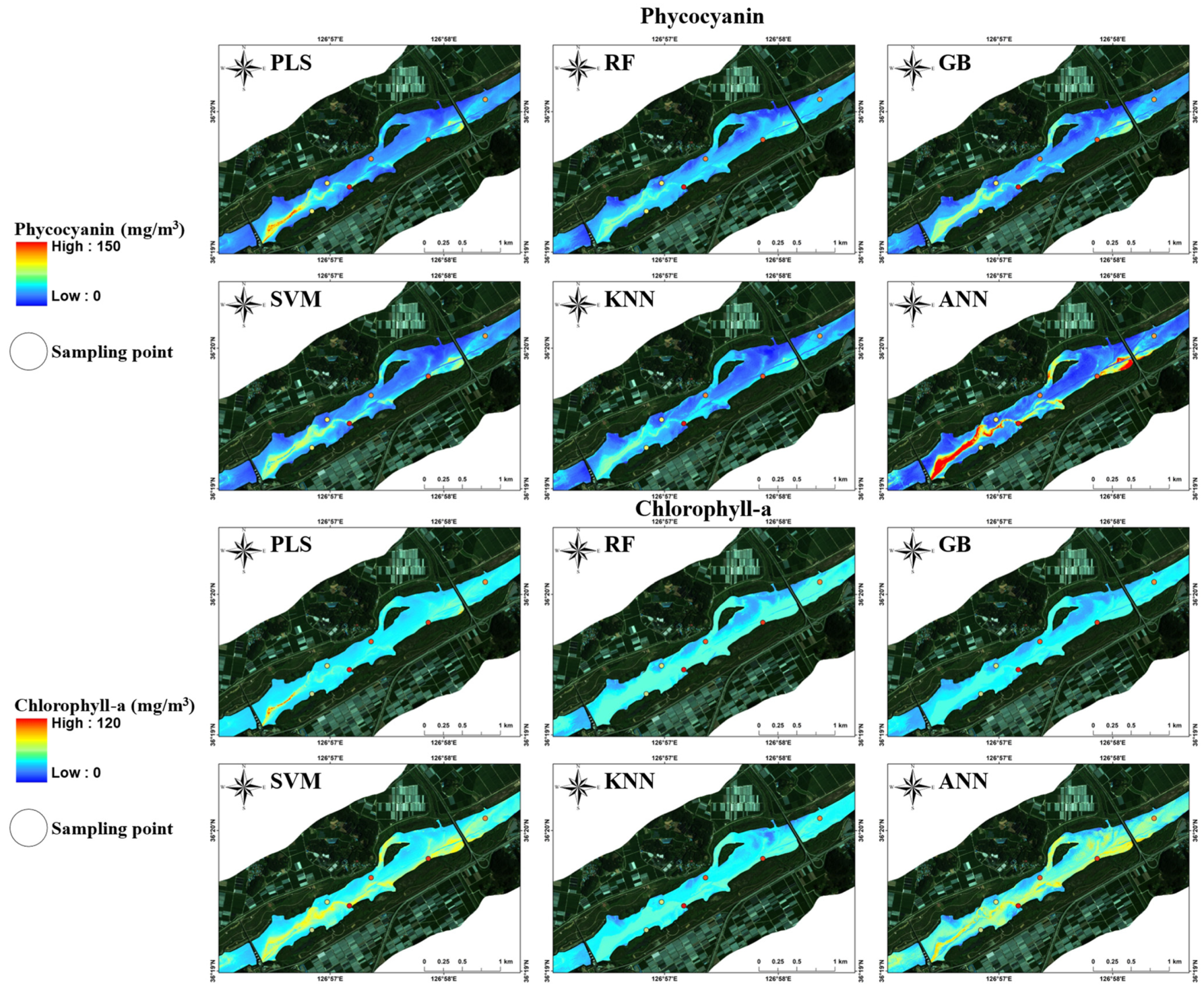
3.3. Baekje Weir Algae Spatial Distribution Generation

The concentrations of the two pigments were estimated by dividing the study area into seven parts for a more granular study. Z1 is the area adjacent to the weir dam, Z2 and Z3 are tributary-affected areas, Z4 and Z6 are river bends, and Z5 and Z7 are locations to check for the effects of any changes in flow velocity according to cross-sectional area (Figure 4).
The spatial distribution characteristics of algae (cyanobacteria) in the BJW were analyzed through the six selected models for the hyperspectral image of 12 August 2016 (Z1), at which time cyanobacteria were predominant (Figure 5). In terms of PC spatial distribution, ANN and PLS more precisely estimated the distribution of high PC concentration near the weir, while the other four models underestimated the PC concentration in the same region. Similarly, ANN, PLS, and KNN performed well in Chl-a spatial distribution; however, in the case of PLS, the Chl-a distribution near the bridge 1 km away from the weir (Z2, Z3) was underestimated.
The spatio-temporal distribution changes of PC and Chl-a over nine sampling days were estimated using the ANN model, which showed good performance in the statistical values and spatial distribution estimation. Figure 6 and Figure 7 show the results, and Appendix A shows the detailed concentration values. The maximum PC and Chl-a concentrations were observed on 12 August 2016, and high concentrations of the two pigments could be seen to be distributed until 24 August 2016. The Chl-a was observed to be above the concentration of 18.05 mg/m3 over the entire monitoring period, but PC was only observed on a specific date (August 2016; September–October 2017) or in a specific section. The concentration of two pigments tended to decrease as it went upstream, and the change in concentration was greater for PC than it is for Chl-a. The overall PC concentration adjacent to the weir dam was high (12 August 2016), and the PC concentration of Z1 (43.80 mg/m3) appeared to be higher than those of Z2 and Z3, which were 34.11 and 30.88 mg/m3, respectively. On the other hand, in the low PC concentration (15 September 2017), Z2 and Z3 of 8.49 and 9.28 mg/m3, respectively, were both similar or higher than Z1 (1.22 mg/m3). Chl-a was generally distributed throughout the entire upstream with an average concentration of 29.42 mg/m3. Unlike Chl-a, high PC concentration were partially observed in Z2, Z3, Z5, and Z6 on August 2016.

4. Discussion

4.1. Band Selection for Inland Cyanobacteria Pigments

Band selection is known to critically affect the performance of the optical algorithm for estimation [59]. The selected six spectral bands included the feature reflectance of cyanobacteria and the water characteristic reflectance (algae, inorganic particles, and suspended solids) (Table 3). The first band, called the green peak, appears in Rgp at around 460–590 nm due to the light reflection by algal cells and the low absorption of Chl-a [25,60]. The bands at 600–630 and 660–680 nm showed minimum reflectance, which was attributed to the strong absorption of both PC (absorption reflectance of PC: Rpa) and Chl-a (absorption reflectance of Chl-a: Rca). The reflectance peak at 640–660 nm appears to be due to the fluorescence characteristics of PC (peak reflectance of PC: Rpp), while the peak at 700–712 nm is a relative peak caused by Chl-a absorption (peak reflectance of Chl-a: Rcp). The last band at 730–784 nm was affected by scattering stemming from the presence of inorganic particles in water (Rwa) [61,62,63]. The four bands in the range from 600–712 nm contain most of the reflectance used in previous studies that estimated the concentrations of PC and Chl-a inland [20,21,22,23,24,25,26]. The two reflectance bands (Rgp and Rwa) improved the performance of the optical algorithm by minimizing the influence of inorganic particles in inland water and removing interference from suspended particles in the green peak reflectance (Table 5) [61,64]. The empirical method using machine learning is generally the most powerful method for estimating a wide range of variables, as it does not require prior understanding of the complex interactions between water and light reflection. However, the performance of this method varies substantially depending on the water quality conditions, locations, and variable ranges from which the data were obtained [65]. Therefore, the optical algorithms in this study obtained high regression performance with the six-reflection band ranges that can correct for the reflection interference effect.

4.2. Cyanobacteria Optical Algorithm Specialized for BJW

The ANN model showed the highest performance in estimating the two pigments. Previous studies that have involved the estimation of two pigments made comparisons according to the use of input spectral bands and the performance of the model. Song et al. [66] estimated the PC concentrations of Central Indiana USA and South Australia using reflection bands of 620 to 630, 685 to 700, and around 555 to 625 nm obtained from Sentinel-3/OLCI and Hyperion satellite data. Partial least squares–ANN and three-band model were applied for PC estimation, and the results were found to be R2 (0.84–0.98). Chang and Vannah [67] estimated the microcystin concentration in Lake Erie using Landsat and MODIS (Landsat: 1–5, 7; MODIS: 1–4, 6, 7). Six reflectance bands obtained from the two satellites were used to construct ANN and genetic programming; the resulting R2 values for the two machine learning models were 0.53 and 0.60, respectively. He et al. [68] estimated the Chl-a concentration in the Gulf of St. Lawrence using 10 bands of MODIS reflectance: 412, 443, 469, 488, 531, 547, 555, 645, 667, and 678 nm. The performances of the five models SVM, ANN, GB, RF, and MLR were compared using R2 values. Among the models, SVM showed the highest R2 values of 0.71 and 0.91 in the training and validation steps, respectively. Zhou et al. [69] estimated Chl-a concentration in Dianshan lake using principal component analysis–ANN to obtain in situ hyperspectral surface reflectance. The R2 values were 0.85 and 0.64 in the training and validation steps, respectively. The ANN model to estimate PC and Chl-a developed in this study showed significantly improved performance over the regression models and offered similar or better performance than the algorithms described in previous studies.

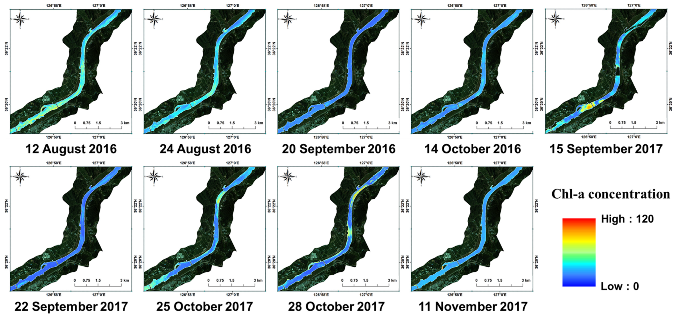
4.3. Spatio-Temporal Distribution Characteristics of Cyanobacteria in BJW

In South Korea, cyanobacterial blooms have intermittently occurred in rivers and reservoirs. However, after the Four Major Rivers Project (2010–2011), many weirs were installed in the major rivers, such as the Nakdong, Geum, and Yeongsan Rivers, which subsequently led to the frequent formation of cyanobacteria blooms, which caused various water quality problems in the weir pools [70]. In the study area, i.e., the BJW of Geum river, algal bloom caused by cyanobacteria has frequently occurred every summer. The maximum air temperatures on the sampling dates (12 August 2016, 24 August 2016, 22 September 2017, and 28 October 2017) when the two cyanobacteria pigments were dominantly distributed in BJW were 36.2, 34.4, 27.0, and 23.8 °C, respectively (Figure A1). The algae growth rate is sensitive to temperature conditions: cyanobacteria in fresh water shows an optimal growth rate of about 30 °C, while other chlorophytes or diatoms have optimal growth rates of around 20–30 °C [71,72,73,74]. In the spatio-temporal change of the two pigments, PC was more sensitive to temperature than Chl-a. In August 2016 (the air and water temperatures were 34.4–36.2 and 30.6–30.9 °C), high PC concentration was widely observed in the BJW under continuous water discharge due to relatively high cyanobacterial growth rates. However, considerably low PC concentrations were collected due to a decrease in the growth rates with decreasing water temperature (23.0 °C) and continuous wash-out by the discharge. Berg and Sutula [75] also reported that if sufficient N and P are provided to allow cyanobacteria to grow, the temperature has the greatest effect on the growth rate.
Chl-a concentration was maintained with relatively high values regardless of sampling dates (e.g., 14 October 2016 vs. 24 August 2016), compared to PC. Based on changes in cyanobacterial and diatom cell density in the BJW [70], relatively high Chl-a and low PC concentrations in September may result from the transition of phytoplankton community [76]. Therefore, it is assumed that there is no noteworthy concentration change compared to PC. The spatial distribution characteristics of PC and Chl-a showed similar patterns when massive cyanobacteria dominated in the upstream of the BJW. In addition, the two pigments are distributed in various patterns in different sections due to the influence of hydrodynamic and tributary river factors. Due to the velocity difference, high concentration is found at the insides of the river bends (Z4, Z6), in large river cross-sections, and at the river boundary, rather than at the center of the river (Z5, Z7). Cyanobacteria grow actively in low velocity and they have a long residence time [77,78,79]. Comparing Z2 and Z3, Z2 distributed a higher concentration due to the tributary river, advective transport and accumulation of biomass at the weir.

5. Conclusions

Based on nine hyperspectral and water quality monitoring campaigns, this study selected major spectral bands related to the effective retrieval of cyanobacteria pigments (i.e., PC, Chl-a) from hyperspectral reflectance data and developed data-driven algorithms for the remote sensing of cyanobacteria. Six reflection band ranges were selected by the random forest feature selection (RFFS) while considering peak and absorption reflectance as affected by PC, Chl-a, SS, and water characteristics. The sensitive reflectance of each band ratio model using both PC and Chl-a showed better performance in the estimation of each pigment than the individual model using each pigment’s sensitive reflectance. This result shows that the two pigments-specific reflectance may be applied simultaneously to construct retrieval models. That is, the selection of relevant reflectance may be critical to the retrieval models, and reflectance bands should be investigated in terms of the pigment sensitivity and improvement of model performance. Overall, this study identified a reflection band that can consider the interference effects of various water characteristics in hyperspectral reflectance imagery, and it therefore provides a useful method for constructing a retrieval model with which to estimate the spatio-temporal concentrations of the main two cyanobacteria pigments (PC and Chl-a). It is expected that future reliable models derived from this study can support the development of efficient management practices for mitigating algal blooms.

Author Contributions

Methodology, W.J. and Y.P.; Writing—Original draft preparation, W.J.; Conceptualization, Y.P.; Data curation, J.P.; Investigation, J.K. and J.H.K.; Validation, K.H.C. and S.P.; Formal analysis, J.-K.S.; and Supervision and Editing, S.K. All authors have read and agreed to the published version of the manuscript.

Funding

This paper was supported by Konkuk University in 2018.

Institutional Review Board Statement

Not applicable.

Informed Consent Statement

Not applicable.

Data Availability Statement

The data presented in this study are available on request from the corresponding author.

Conflicts of Interest

The authors declare no conflict of interest.

Appendix A. Statistics of Phycocyanin and Chlorophyll-a Spatial Concentration

Table A1. Summary of ANN-estimated phycocyanin and chlorophyll-a concentrations of the seven sections.
PigmentDateZone
1234567Overall
MEANSTDMEANSTDMEANSTDMEANSTDMEANSTDMEANSTDMEANSTDMean
PC12 August 201643.8034.7034.1130.1630.8820.3022.1012.8537.2026.5333.2423.4625.7918.4032.45
24 August 201636.1324.6849.9215.4649.2124.1139.8213.8733.0816.2320.785.9811.843.5234.40
20 September 20164.544.573.823.933.673.343.283.744.573.695.964.156.494.834.62
14 October 20164.514.434.265.355.467.197.457.343.612.813.762.544.484.324.79
15 September 20171.222.018.497.789.285.8910.134.523.093.133.743.701.321.765.32
22 September 201711.999.2511.458.828.637.222.512.462.493.053.633.805.934.696.66
25 October 201711.079.5112.7310.736.218.5414.918.6511.168.1012.668.335.375.1410.59
28 October 201719.8710.7215.2613.8012.3214.4210.129.8212.819.5912.977.4110.087.8713.35
11 November 20173.034.922.784.182.273.152.422.781.592.452.042.862.913.862.43
Avg.15.1311.6415.8711.1314.2110.4612.537.3412.188.4010.976.928.256.0412.73
Chl-a12 August 201648.3515.2950.4515.0547.1411.8145.5913.0241.8711.1537.7112.1333.929.7743.57
24 August 201636.3410.2935.128.1839.689.0147.149.1137.1010.5530.8211.6028.519.4736.39
20 September 201622.369.4321.997.0123.056.8120.444.6519.093.9917.312.9417.023.2220.18
14 October 201624.038.0123.786.9925.068.3329.558.2927.094.6924.283.5126.615.2625.77
15 September 201733.0912.8352.5624.6540.8724.3627.298.6830.4212.1430.039.6835.705.2035.71
22 September 201718.696.1516.163.3615.674.7518.043.8717.815.3518.415.9121.555.0818.05
25 October 201737.8513.8723.5412.5124.659.9526.3211.7625.4210.4337.5116.9926.867.7328.88
28 October 201723.6113.4323.4516.4424.8815.7824.1512.9832.5221.7147.0529.1126.2718.2028.85
11 November 201730.037.1029.9313.5825.675.7825.273.6826.194.5227.807.3726.654.8227.36
Avg.30.4810.7130.7711.9829.6310.7329.318.4528.619.3930.1011.0327.017.6429.42

Appendix B. July to November Weather and Water Quality Features in Baekje Weir

Figure A1. Temporal variations in streamflow; Total nitrogen (TN): Total phosphorus ratio (TP). TN and TP concentrations in air, and water temperatures during the 2016 to 2017 period; the nine sampling dates are indicated by magenta rectangles; PC and Chl-a concentration box plot of each sampling date.
Remotesensing 14 01754 g0a1

References

  1. O’Neil, J.M.; Davis, T.W.; Burford, M.A.; Gobler, C.J. The rise of harmful cyanobacteria blooms: The potential roles of eutrophication and climate change. Harmful Algae 2012, 14, 313–334. [Google Scholar] [CrossRef]
  2. Brooks, B.W.; Lazorchak, J.M.; Howard, M.D.A.; Johnson, M.V.V.; Morton, S.L.; Perkins, D.A.K.; Reavie, E.D.; Scott, G.I.; Smith, S.A.; Steevens, J.A. Are harmful algal blooms becoming the greatest inland water quality threat to public health and aquatic ecosystems? Environ. Toxicol. Chem. 2016, 35, 6–13. [Google Scholar] [CrossRef] [PubMed]
  3. Hudnell, H.K. The state of U.S. freshwater harmful algal blooms assessments, policy and legislation. Toxicon 2010, 55, 1024–1034. [Google Scholar] [CrossRef] [PubMed]
  4. Chapra, S.C.; Canale, R.P.; Amy, G.L. Empirical Models for Disinfection By-Products in Lakes and Reservoirs. J. Environ. Eng. 1997, 123, 1–12. [Google Scholar] [CrossRef]
  5. Matthews, M.W.; Bernard, S.; Robertson, L. An algorithm for detecting trophic status (chlorophyll-a), cyanobacterial-dominance, surface scums and floating vegetation in inland and coastal waters. Remote Sens. Environ. 2012, 124, 637–652. [Google Scholar] [CrossRef]
  6. Matthews, M.W.; Odermatt, D. Improved algorithm for routine monitoring of cyanobacteria and eutrophication in inland and near-coastal waters. Remote Sens. Environ. 2015, 156, 374–382. [Google Scholar] [CrossRef]
  7. Su, T.C.; Chou, H.T. Application of multispectral sensors carried on unmanned aerial vehicle (UAV) to trophic state mapping of small reservoirs: A case study of Tain-Pu reservoir in Kinmen, Taiwan. Remote Sens. 2015, 7, 10078–10097. [Google Scholar] [CrossRef] [Green Version]
  8. Binding, C.E.; Greenberg, T.A.; Jerome, J.H.; Bukata, R.P.; Letourneau, G. An assessment of MERIS algal products during an intense bloom in Lake of the Woods. J. Plankton Res. 2011, 33, 793–806. [Google Scholar] [CrossRef] [Green Version]
  9. Duan, H.; Ma, R.; Zhang, Y.; Loiselle, S.A.; Xu, J.; Zhao, C.; Zhou, L.; Shang, L. A new three-band algorithm for estimating chlorophyll concentrations in turbid inland lakes. Environ. Res. Lett. 2010, 5, 044009. [Google Scholar] [CrossRef]
  10. Shi, K.; Zhang, Y.; Qin, B.; Zhou, B. Remote sensing of cyanobacterial blooms in inland waters: Present knowledge and future challenges. Sci. Bull. 2019, 64, 1540–1556. [Google Scholar] [CrossRef] [Green Version]
  11. Kim, Y.H.; Im, J.; Ha, H.K.; Choi, J.K.; Ha, S. Machine learning approaches to coastal water quality monitoring using GOCI satellite data. GISci. Remote Sens. 2014, 51, 158–174. [Google Scholar] [CrossRef]
  12. Zhang, Y.; Pulliainen, J.; Koponen, S.; Hallikainen, M. Application of an empirical neural network to surface water quality estimation in the Gulf of Finland using combined optical data and microwave data. Remote Sens. Environ. 2002, 81, 327–336. [Google Scholar] [CrossRef]
  13. Kutser, T.; Herlevi, A.; Kallio, K.; Arst, H. A hyperspectral model for interpretation of passive optical remote sensing data from turbid lakes. Sci. Total Environ. 2001, 268, 47–58. [Google Scholar] [CrossRef]
  14. Lunetta, R.S.; Knight, J.F.; Paerl, H.W.; Streicher, J.J.; Peierls, B.L.; Gallo, T.; Lyon, J.G.; Mace, T.H.; Buzzelli, C.P. Measurement of water colour using AVIRIS imagery to assess the potential for an operational monitoring capability in the Pamlico Sound Estuary, USA. Int. J. Remote Sens. 2009, 30, 3291–3314. [Google Scholar] [CrossRef] [PubMed]
  15. Li, L.; Sengpiel, R.E.; Pascual, D.L.; Tedesco, L.P.; Wilson, J.S.; Soyeux, A. Using hyperspectral remote sensing to estimate chlorophyll-a and phycocyanin in a mesotrophic reservoir. Int. J. Remote Sens. 2010, 31, 4147–4162. [Google Scholar] [CrossRef]
  16. Pyo, J.C.; Duan, H.; Baek, S.; Kim, M.S.; Jeon, T.; Kwon, Y.S.; Lee, H.; Cho, K.H. A convolutional neural network regression for quantifying cyanobacteria using hyperspectral imagery. Remote Sens. Environ. 2019, 233, 111350. [Google Scholar] [CrossRef]
  17. Pyo, J.C.; Duan, H.; Ligaray, M.; Kim, M.; Baek, S.; Kwon, Y.S.; Lee, H.; Kang, T.; Kim, K.; Cha, Y.K.; et al. An integrative remote sensing application of stacked autoencoder for atmospheric correction and cyanobacteria estimation using hyperspectral imagery. Remote Sens. 2020, 12, 1073. [Google Scholar] [CrossRef] [Green Version]
  18. Keller, S.; Maier, P.M.; Riese, F.M.; Norra, S.; Holbach, A.; Börsig, N.; Wilhelms, A.; Moldaenke, C.; Zaake, A.; Hinz, S. Hyperspectral data and machine learning for estimating CDOM, chlorophyll a, diatoms, green algae and turbidity. Int. J. Environ. Res. Public Health 2018, 15, 1881. [Google Scholar] [CrossRef] [Green Version]
  19. Šindelář, R.; Babuška, R. Input selection for nonlinear regression models. IEEE Trans. Fuzzy Syst. 2004, 12, 688–696. [Google Scholar] [CrossRef]
  20. Dekker, A.G. Detection of Optical Water Quality Parameters for Eutrophic Waters by High Resolution Remote Sensing; Institute for Environmental Studies: Amsterdam, The Netherlands, 1993. [Google Scholar]
  21. Mishra, S.; Mishra, D.R.; Schluchter, W.M. A novel algorithm for predicting phycocyanin concentrations in cyanobacteria: A proximal hyperspectral remote sensing approach. Remote Sens. 2009, 1, 758–775. [Google Scholar] [CrossRef] [Green Version]
  22. Simis, S.G.H.; Peters, S.W.M.; Gons, H.J. Remote sensing of the cyanobacterial pigment phycocyanin in turbid inland water. Limnol. Oceanogr. 2005, 50, 237–245. [Google Scholar] [CrossRef]
  23. Kallio, K.; Kutser, T.; Hannonen, T.; Koponen, S.; Pulliainen, J.; Vepsäläinen, J.; Pyhälahti, T. Retrieval of water quality from airborne imaging spectrometry of various lake types in different seasons. Sci. Total Environ. 2001, 268, 59–77. [Google Scholar] [CrossRef]
  24. Shafique, N.A.; Fulk, F.; Autrey, B.C.; Flotemersch, J. Water area extraction using geocoded high resolution imagery of TerraSAR-X radar satellite in cloud prone Brahmaputra River valley. J. Geomat. 2009, 3, 9–12. [Google Scholar]
  25. Ogashawara, I.; Mishra, D.R.; Mishra, S.; Curtarelli, M.P.; Stech, J.L. A performance review of reflectance based algorithms for predicting phycocyanin concentrations in inland waters. Remote Sens. 2013, 5, 4774–4798. [Google Scholar] [CrossRef] [Green Version]
  26. Schalles, J.F.; Yacobi, Y.Z. Remote detection and seasonal patterns of phycocyanin, carotenoid and chlorophyll pigments in eutrophic waters. Ergeb. Limnol. 2000, 55, 153–168. [Google Scholar]
  27. Soja-Woźniak, M.; Darecki, M.; Wojtasiewicz, B.; Bradtke, K. Laboratory measurements of remote sensing reflectance of selected phytoplankton species from the Baltic Sea. Oceanologia 2018, 60, 86–96. [Google Scholar] [CrossRef]
  28. Hestir, E.L.; Brando, V.E.; Bresciani, M.; Giardino, C.; Matta, E.; Villa, P.; Dekker, A.G. Measuring freshwater aquatic ecosystems: The need for a hyperspectral global mapping satellite mission. Remote Sens. Environ. 2015, 167, 181–195. [Google Scholar] [CrossRef] [Green Version]
  29. Yan, Y.; Bao, Z.; Shao, J. Phycocyanin concentration retrieval in inland waters: A comparative review of the remote sensing techniques and algorithms. J. Great Lakes Res. 2018, 44, 748–755. [Google Scholar] [CrossRef]
  30. Pyo, J.C.; Ligaray, M.; Kwon, Y.S.; Ahn, M.H.; Kim, K.; Lee, H.; Kang, T.; Cho, S.B.; Park, Y.; Cho, K.H. High-spatial resolution monitoring of phycocyanin and chlorophyll-a using airborne hyperspectral imagery. Remote Sens. 2018, 10, 1180. [Google Scholar] [CrossRef] [Green Version]
  31. Berk, A.; Conforti, P.; Kennett, R.; Perkins, T.; Hawes, F.; Van Den Bosch, J. MODTRAN® 6: A major upgrade of the MODTRAN® radiative transfer code. In Proceedings of the Workshop on Hyperspectral Image and Signal Processing, Evolution in Remote Sensing, Lausanne, Switzerland, 24–27 June 2014; pp. 1–4. [Google Scholar]
  32. Pyo, J.; Ha, S.; Pachepsky, Y.A.; Lee, H.; Ha, R.; Nam, G.; Kim, M.S.; Im, J.; Cho, K.H. Chlorophyll- a concentration estimation using three difference bio-optical algorithms, including a correction for the low-concentration range: The case of the Yiam reservoir, Korea. Remote Sens. Lett. 2016, 7, 407–416. [Google Scholar] [CrossRef]
  33. Pyo, J.C.; Pachepsky, Y.; Baek, S.S.; Kwon, Y.S.; Kim, M.J.; Lee, H.; Park, S.; Cha, Y.K.; Ha, R.; Nam, G.; et al. Optimizing semi-analytical algorithms for estimating chlorophyll-a and phycocyanin concentrations in inland waters in Korea. Remote Sens. 2017, 9, 542. [Google Scholar] [CrossRef] [Green Version]
  34. Sarada, R.; Pillai, M.G.; Ravishankar, G.A. Phycocyanin from Spirulina sp.: Influence of processing of biomass on phycocyanin yield, analysis of efficacy of extraction methods and stability studies on phycocyanin. Process Biochem. 1999, 34, 795–801. [Google Scholar] [CrossRef]
  35. Le Bris, A.; Chehata, N.; Briottet, X.; Paparoditis, N. A random forest class memberships based wrapper band selection criterion: Application to hyperspectral. Int. Geosci. Remote Sens. Symp. 2015, 2015, 1112–1115. [Google Scholar] [CrossRef] [Green Version]
  36. Jaiswal, J.K.; Samikannu, R. Application of Random Forest Algorithm on Feature Subset Selection and Classification and Regression. In Proceedings of the 2017 World Congress on Computing and Communication Technologies (WCCCT), Tiruchirappalli, India, 2–4 February 2017; pp. 65–68. [Google Scholar] [CrossRef]
  37. Reinart, A.; Kutser, T. Comparison of different satellite sensors in detecting cyanobacterial bloom events in the Baltic Sea. Remote Sens. Environ. 2006, 102, 74–85. [Google Scholar] [CrossRef]
  38. Menken, K.D.; Brezonik, P.L.; Bauer, M.E. Influence of chlorophyll and colored dissolved organic matter (CDOM) on lake reflectance spectra: Implications for measuring lake properties by remote sensing. Lake Reserv. Manag. 2006, 22, 179–190. [Google Scholar] [CrossRef] [Green Version]
  39. Brezonik, P.L.; Olmanson, L.G.; Finlay, J.C.; Bauer, M.E. Factors affecting the measurement of CDOM by remote sensing of optically complex inland waters. Remote Sens. Environ. 2015, 157, 199–215. [Google Scholar] [CrossRef]
  40. Ha, N.T.T.; Thao, N.T.P.; Koike, K.; Nhuan, M.T. Selecting the best band ratio to estimate chlorophyll-a concentration in a tropical freshwater lake using sentinel 2A images from a case study of Lake Ba Be (Northern Vietnam). ISPRS Int. J. Geo-Inf. 2017, 6, 290. [Google Scholar] [CrossRef]
  41. Gitelson, A.A.; Schalles, J.F.; Rundquist, D.C.; Schiebe, F.R.; Yacobi, Y.Z. Comparative reflectance properties of algal cultures with manipulated densities. J. Appl. Phycol. 1999, 11, 345–354. [Google Scholar] [CrossRef]
  42. Quibell, G. The effect of suspended sediment on reflectance from freshwater algae. Int. J. Remote Sens. 1991, 12, 177–182. [Google Scholar] [CrossRef]
  43. Geladi, P.; Kowalski, B.R. Partial least-squares regression: A tutorial. Anal. Chim. Acta 1986, 185, 1–17. [Google Scholar] [CrossRef]
  44. Abdi, H. Partial least square regression (PLS regression). Encycl. Res. Methods Soc. Sci. 2003, 6, 792–795. [Google Scholar] [CrossRef]
  45. Guo, L.; Chehata, N.; Mallet, C.; Boukir, S. Relevance of airborne lidar and multispectral image data for urban scene classification using Random Forests. ISPRS J. Photogramm. Remote Sens. 2011, 66, 56–66. [Google Scholar] [CrossRef]
  46. Rodriguez-Galiano, V.; Sanchez-Castillo, M.; Chica-Olmo, M.; Chica-Rivas, M. Machine learning predictive models for mineral prospectivity: An evaluation of neural networks, random forest, regression trees and support vector machines. Ore Geol. Rev. 2015, 71, 804–818. [Google Scholar] [CrossRef]
  47. Elith, J.; Leathwick, J.R.; Hastie, T. A working guide to boosted regression trees. J. Anim. Ecol. 2008, 77, 802–813. [Google Scholar] [CrossRef] [PubMed]
  48. Khazaee Poul, A.; Shourian, M.; Ebrahimi, H. A Comparative Study of MLR, KNN, ANN and ANFIS Models with Wavelet Transform in Monthly Stream Flow Prediction. Water Resour. Manag. 2019, 33, 2907–2923. [Google Scholar] [CrossRef]
  49. Vapnik, V.; Guyon, I.; Hastie, T.; Rosset, S.; Zhu, J.; Tibshirani, R. Support vector machines. Mach. Learn 1995, 20, 273–297. [Google Scholar]
  50. Coulibaly, M.S.K.P. Application of support vector machine in power system. Study Dyn. Syst. 2006, 11, 199–205. [Google Scholar] [CrossRef]
  51. Mohammadpour, R.; Shaharuddin, S.; Chang, C.K.; Zakaria, N.A.; Ghani, A.A.; Chan, N.W. Prediction of water quality index in constructed wetlands using support vector machine. Environ. Sci. Pollut. Res. 2015, 22, 6208–6219. [Google Scholar] [CrossRef]
  52. Zou, J.; Han, Y.; So, S.S. Overview of artificial neural networks. Methods Mol. Biol. 2008, 458, 15–23. [Google Scholar] [CrossRef]
  53. Palani, S.; Liong, S.Y.; Tkalich, P. An ANN application for water quality forecasting. Mar. Pollut. Bull. 2008, 56, 1586–1597. [Google Scholar] [CrossRef]
  54. Pedregosa, F.; Varoquaux, G.; Gramfort, A.; Michel, V.; Thirion, B.; Grisel, O.; Duchesnay, E. Scikit-learn: Machine learning in Python. J. Mach. Learn. Res. 2011, 12, 2825–2830. [Google Scholar]
  55. Santhi, C.; Arnold, J.G.; Williams, J.R.; Dugas, W.A.; Srinivasan, R.; Hauck, L.M. Validation of the swat model on a large rwer basin with point and nonpoint sources 1. JAWRA J. Am. Water Resour. Assoc. 2001, 37, 1169–1188. [Google Scholar] [CrossRef]
  56. Moriasi, D.N.; Arnold, J.G.; Van Liew, M.W.; Bingner, R.L.; Harmel, R.D.; Veith, T.L. Model evaluation guidelines for systematic quantification of accuracy in watershed simulations. Trans. ASABE 2007, 50, 885–900. [Google Scholar] [CrossRef]
  57. Nash, J.E.; Sutcliffe, J.V. River flow forecasting through conceptual models part I—A discussion of principles. J. Hydrol. 1970, 10, 282–290. [Google Scholar] [CrossRef]
  58. Singh, J.; Knapp, H.V.; Arnold, J.G.; Demissie, M. Hydrological modeling of the Iroquois River watershed using HSPF and SWAT. J. Am. Water Resour. Assoc. 2005, 41, 343–360. [Google Scholar] [CrossRef]
  59. Oki, K. Why is the ratio of reflectivity effective for chlorophyll estimation in the lake water? Remote Sens. 2010, 2, 1722–1730. [Google Scholar] [CrossRef] [Green Version]
  60. Vincent, R.K.; Qin, X.; McKay, R.M.L.; Miner, J.; Czajkowski, K.; Savino, J.; Bridgeman, T. Phycocyanin detection from LANDSAT TM data for mapping cyanobacterial blooms in Lake Erie. Remote Sens. Environ. 2004, 89, 381–392. [Google Scholar] [CrossRef]
  61. Yacobi, Y.Z.; Moses, W.J.; Kaganovsky, S.; Sulimani, B.; Leavitt, B.C.; Gitelson, A.A. NIR-red reflectance-based algorithms for chlorophyll-a estimation in mesotrophic inland and coastal waters: Lake Kinneret case study. Water Res. 2011, 45, 2428–2436. [Google Scholar] [CrossRef] [Green Version]
  62. Augusto-Silva, P.B.; Ogashawara, I.; Barbosa, C.C.F.; de Carvalho, L.A.S.; Jorge, D.S.F.; Fornari, C.I.; Stech, J.L. Analysis of MERIS reflectance algorithms for estimating chlorophyll-a concentration in a Brazilian reservoir. Remote Sens. 2014, 6, 11689–11707. [Google Scholar] [CrossRef] [Green Version]
  63. Rundquist, D.C.; Han, L.; Schalles, J.F.; Peake, J.S. Remote measurement of algal chlorophyll in surface waters: The case for the first derivative of reflectance near 690 nm. Photogramm. Eng. Remote Sens. 1996, 62, 195–200. [Google Scholar]
  64. Schalles, J.F.; Rundquist, D.C.; Schiebe, F.R. The influence of suspended clays on phytoplankton reflectance signatures and the remote estimation of chlorophyll. SIL Proc. 2001, 27, 3619–3625. [Google Scholar] [CrossRef]
  65. Sagan, V.; Peterson, K.T.; Maimaitijiang, M.; Sidike, P.; Sloan, J.; Greeling, B.A.; Maalouf, S.; Adams, C. Monitoring inland water quality using remote sensing: Potential and limitations of spectral indices, bio-optical simulations, machine learning, and cloud computing. Earth-Sci. Rev. 2020, 205, 103187. [Google Scholar] [CrossRef]
  66. Song, K.; Li, L.; Tedesco, L.P.; Li, S.; Hall, B.E.; Du, J. Remote quantification of phycocyanin in potable water sources through an adaptive model. ISPRS J. Photogramm. Remote Sens. 2014, 95, 68–80. [Google Scholar] [CrossRef]
  67. Chang, N.-B.; Vannah, B. Intercomparisons between empirical models with data fusion techniques for monitoring water quality in a large lake. In Proceedings of the 2013 10th IEEE International Conference on Networking, Sensing and Control (ICNSC 2013), Evry, France, 10–12 April 2013; pp. 258–263. [Google Scholar] [CrossRef]
  68. He, J.; Chen, Y.; Wu, J.; Stow, D.A.; Christakos, G. Space-time chlorophyll-a retrieval in optically complex waters that accounts for remote sensing and modeling uncertainties and improves remote estimation accuracy. Water Res. 2020, 171, 115403. [Google Scholar] [CrossRef]
  69. Zhou, L.; Ma, W.; Zhang, H.; Li, L.; Tang, L. Developing a PCA–ANN model for predicting chlorophyll a concentration from field hyperspectral measurements in dianshan lake, China. Water Qual. Expo. Health 2015, 7, 591–602. [Google Scholar] [CrossRef]
  70. Kim, S.; Chung, S.; Park, H.; Cho, Y.; Lee, H. Analysis of environmental factors associated with cyanobacterial dominance after river weir installation. Water 2019, 11, 1163. [Google Scholar] [CrossRef] [Green Version]
  71. Konopka, A.; Brock, T.D. Effect of temperature on blue-green algae (Cyanobacteria) in Lake Mendota. Appl. Environ. Microbiol. 1978, 36, 572–576. [Google Scholar] [CrossRef] [Green Version]
  72. Lürling, M.; Eshetu, F.; Faassen, E.J.; Kosten, S.; Huszar, V.L.M. Comparison of cyanobacterial and green algal growth rates at different temperatures. Freshw. Biol. 2013, 58, 552–559. [Google Scholar] [CrossRef]
  73. Nalley, J.O.; O’Donnell, D.R.; Litchman, E. Temperature effects on growth rates and fatty acid content in freshwater algae and cyanobacteria. Algal Res. 2018, 35, 500–507. [Google Scholar] [CrossRef]
  74. Paerl, H.W.; Paul, V.J. Climate change: Links to global expansion of harmful cyanobacteria. Water Res. 2012, 46, 1349–1363. [Google Scholar] [CrossRef]
  75. Berg, M.; Sutula, M. Factors Affecting Growth of Cyanobacteria. Monaldi Arch. Chest Dis. Pulm. Ser. 2015, 59, 103–107. [Google Scholar]
  76. Dev, P.J.; Sukenik, A.; Mishra, D.R.; Ostrovsky, I. Cyanobacterial pigment concentrations in inland waters: Novel semi-analytical algorithms for multi- and hyperspectral remote sensing data. Sci. Total Environ. 2022, 805, 150423. [Google Scholar] [CrossRef]
  77. Park, Y.; Pyo, J.C.; Kwon, Y.S.; Cha, Y.K.; Lee, H.; Kang, T.; Cho, K.H. Evaluating physico-chemical influences on cyanobacterial blooms using hyperspectral images in inland water, Korea. Water Res. 2017, 126, 319–328. [Google Scholar] [CrossRef]
  78. Ha, K.; Cho, E.A.; Kim, H.W.; Joo, G.J. Microcystis bloom formation in the lower Nakdong River, South Korea: Importance of hydrodynamics and nutrient loading. Mar. Freshw. Res. 1999, 50, 89–94. [Google Scholar] [CrossRef]
  79. Oliver, R.L.; Ganf, G.G. Freshwater blooms. In The Ecology of Cyanobacteria; Springer: Berlin/Heidelberg, Germany, 2000; pp. 149–194. [Google Scholar]
Figure 1. Map of airborne hyperspectral scanning area, Location of Baekje weir and monitoring points indicated, respectively, by red line and marks (2016: triangles; 2017: pentagons).
Remotesensing 14 01754 g001
Figure 2. A hyperspectral reflectance curve extracted from a sampling point. The positions of peak and absorption were shifted according to the concentration of the water quality factors. (a) PC, 146.99; Chl-a, 111.4; and SS, 40.14. (b) PC, 54.81; Chl-a, 66.18; and SS, 16.93. (c) PC, 1.54; Chl-a, 60.88; and SS, 16.67. (d) PC, 15.89; Chl-a, 51.54; and SS, 9.47. (e) PC, 100; Chl-a, 36.78; and SS, 13.2. (f) PC, 8.93; Chl-a, 17.52; and SS, 7.33.
Remotesensing 14 01754 g002
Figure 3. Comparison of concentration of two pigments (PC, Phycocyanin; Chl-a, Chlorophyll-a) between observed and estimated values from each of the following optimized regression methods: (a) partial least square, (b) random forest, (c) gradient boosting regression tree, (d) support vector machine, (e) K-nearest neighbors, and (f) artificial neural network. Training is denoted by a black closed circle. Validation is denoted by a red open circle.
Remotesensing 14 01754 g003
Figure 4. Map of the cyanobacteria distribution divided into seven sections according to the hydrodynamic conditions and tributary rivers.
Remotesensing 14 01754 g004
Figure 5. Comparison map of phycocyanin (PC) and chlorophyll-a (Chl-a) concentration distribution by six optimized regression models from hyperspectral imagery near Baekje weir on 12 August 2016, when cyanobacteria were predominantly distributed; sampling point is marked with PC and Chl-a concentration.
Remotesensing 14 01754 g005
Figure 6. Spatio-temporal change estimation of phycocyanin concentration by applying artificial neural network to the hyperspectral imagery of the nine sampling dates.
Remotesensing 14 01754 g006
Figure 7. Spatio-temporal change estimation of chlorophyll-a concentration by applying artificial neural network to the hyperspectral imagery of the nine sampling dates.
Remotesensing 14 01754 g007
Table 1. Descriptive two-year water quality sampling statistics (mg/m3) of Baekje weir.
DateNumber of SamplesPCChlorophyll-a
* Avg.* Std.MinMaxAvg.Std.MinMax
12 August 20161835.4636.106.04146.9940.6523.3814.19111.40
24 August 20162038.0723.5812.25100.0037.248.0225.9561.44
20 September 2016171.230.270.831.6425.5111.3211.8560.88
14 October 2016200.330.170.190.8828.219.3813.7446.17
15 September 2017128.340.667.419.6647.288.5430.2461.52
22 September 20171212.633.967.6421.6917.573.8014.0827.89
25 October 2017123.510.672.644.5613.182.8510.5620.92
28 October 2017124.354.521.1814.7710.542.288.4516.73
11 November 2017110.350.140.230.7122.006.7612.7638.43
* Avg.: Average, * Std.: Standard deviation.
Table 2. Result of band selection according to PC and Chl-a concentration using random forest feature importance.
PigmentConcentration (mg/L)No. of Bands SelectedBand (nm)
PC0–314452, 470, 484, 604, 674, 684, 708, 712, 717, 727, 784, 789, 794, 799
3–1514466, 525, 679, 741, 746, 751, 755, 760, 765, 770, 775, 779, 784, 789
15–14720457, 461, 470, 475, 488, 497, 502, 507, 511, 516, 520, 525, 529, 543, 665, 670, 674, 693, 717, 784
Chl-a0–2021566, 571, 580, 585, 590, 604, 646, 651, 655, 660, 665, 670, 674, 698, 703, 708, 717, 722, 727, 784, 789
20–3525452, 466, 470, 488, 507, 511, 516, 520, 525, 529, 539, 543, 552, 674, 689, 722, 736, 751, 755, 760, 770, 775, 784, 789, 794
35–11122488, 548, 590, 599, 604, 627, 646, 651, 655, 689, 698, 703, 708, 712, 717, 731, 736, 741, 755, 779, 789, 794
Table 3. Cyanobacteria key features’ reflectance bands (nm).
PigmentTypeMIN MAX
PCpeak641.18~655.35Rpp
* abs.603.60~631.76Rpa
Chl-apeak698.04~712.33Rcp
abs.664.81~679.03Rca
Greenpeak465.74~589.58Rgp
Waterabs.731.42~784.11Rwa
* abs.: absorbance.
Table 4. Performances of six data-driven models on estimation of two pigments in terms of different input spectral band combinations.
Case *Pigment TrainingValidation
MethodR2NSERMSER2NSERMSE
* Case 1PCPLS0.600.6014.690.340.339.46
RF0.730.7011.550.510.4312.84
GB0.790.7310.550.590.5412.13
SVM0.680.8112.500.710.4319.58
KNN0.690.6913.400.510.348.06
ANN0.800.7611.410.680.499.99
Avg.0.710.7212.350.560.4312.01
* Case 2Chl-aPLS0.29−1.4413.730.28−6.7710.98
RF0.46−1.0211.370.35−4.1015.97
GB0.670.189.620.300.1114.00
SVM0.48−0.4611.770.340.0611.14
KNN0.38−1.1811.090.30−4.7518.05
ANN0.520.4811.600.430.0512.09
Avg.0.47−0.5711.530.33−2.5713.70
* Case 3PCPLS0.690.6910.980.560.6418.09
RF0.770.769.630.710.7415.38
GB0.850.847.780.740.7415.32
SVM0.700.6911.140.680.7016.35
KNN0.740.7310.390.670.7315.61
ANN0.810.6511.720.790.8411.92
Avg.0.760.7310.270.690.7315.45
Chl-aPLS0.350.3510.810.290.7917.79
RF0.590.588.710.420.8315.97
GB0.580.539.160.430.8216.63
SVM0.470.459.940.460.8515.08
KNN0.530.519.390.460.8316.12
ANN0.800.796.090.670.9211.38
Avg.0.550.549.020.460.8415.50
* Case 1: PC estimation with PC feature spectral reflectance band, * Case 2: Chl-a estimation with Chl-a feature spectral reflectance band, and * Case 3: PC and Chl-a estimation with combined feature reflectance of two pigments.
Table 5. Comparison of change in artificial neural network (ANN) performance according to input band change.
PigmentCaseTrainingValidation
R2NSERMSER2NSERMSE
PCA0.8050.7999.4470.7190.18814.881
B0.8690.8487.1760.7170.32814.438
C0.7950.6669.9740.5970.21616.813
Chl-aA0.5440.2889.3600.6040.03012.898
B0.5640.2208.9340.587−0.99214.075
C0.5650.2729.0940.480−1.76314.995
A: Reflection of water absorption of 731.42–784.11 nm removed from Origin ANN input data. B: Reflection of green peak of 465.74–589.58 nm removed from Origin ANN input data. C: Reflection of water absorption and green peak removed from Origin ANN input data.
Publisher’s Note: MDPI stays neutral with regard to jurisdictional claims in published maps and institutional affiliations.

