
Giant Planet Atmospheres: Dynamics and Variability from UV to Near-IR Hubble and Adaptive Optics Imaging

 , , , and
Abstract
1. Introduction
2. History of High-Resolution Imaging
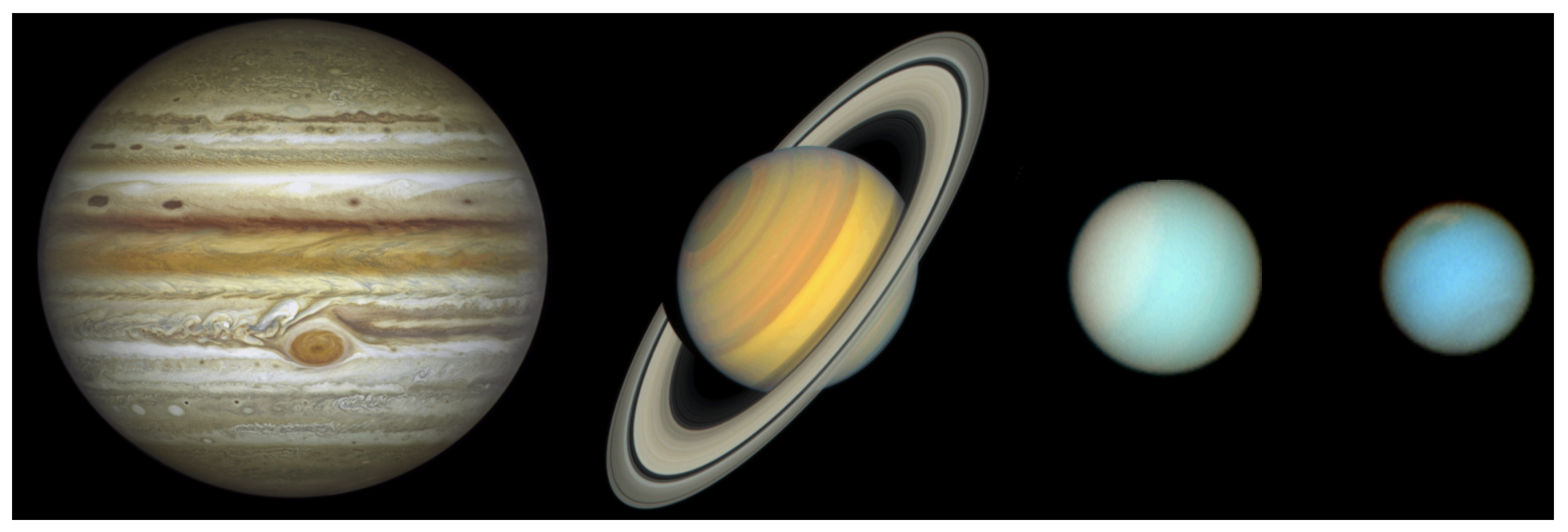
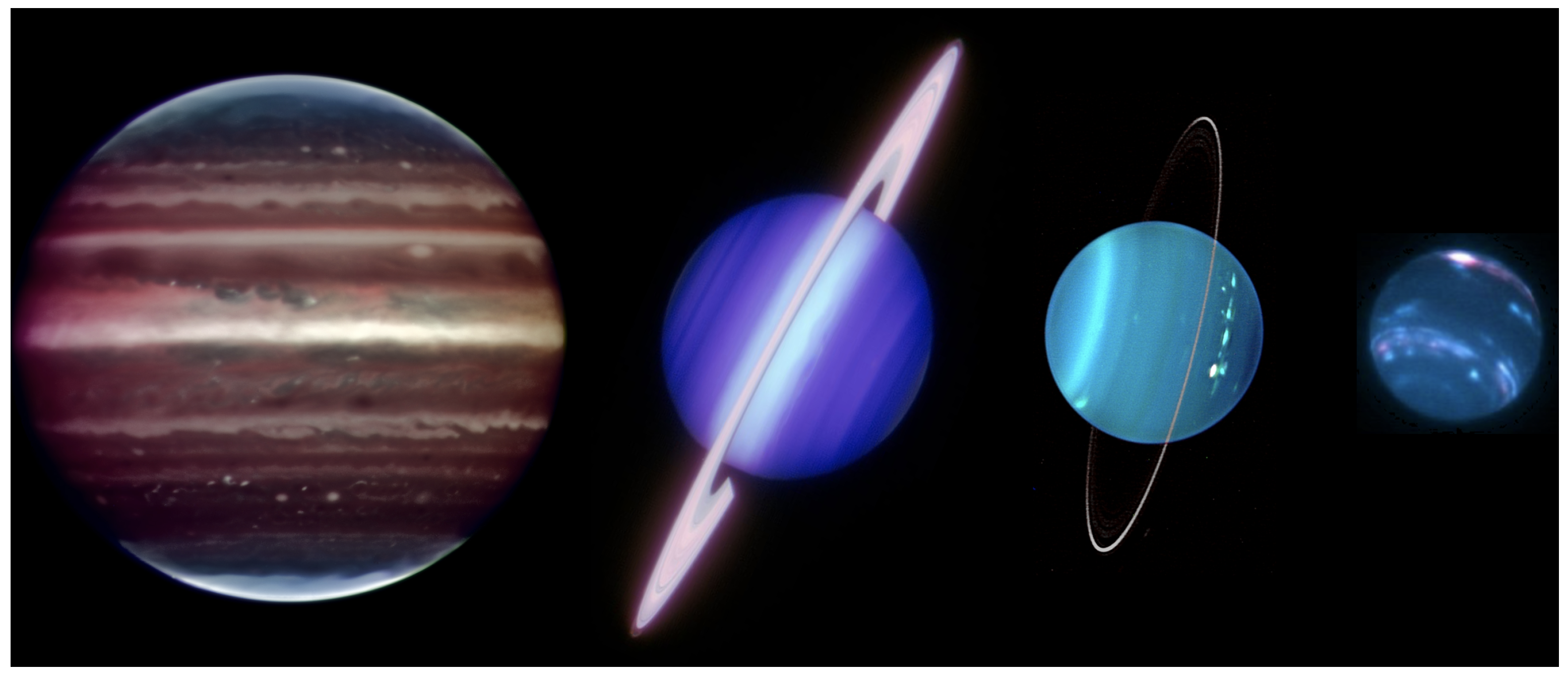
3. Cloud Top Appearance

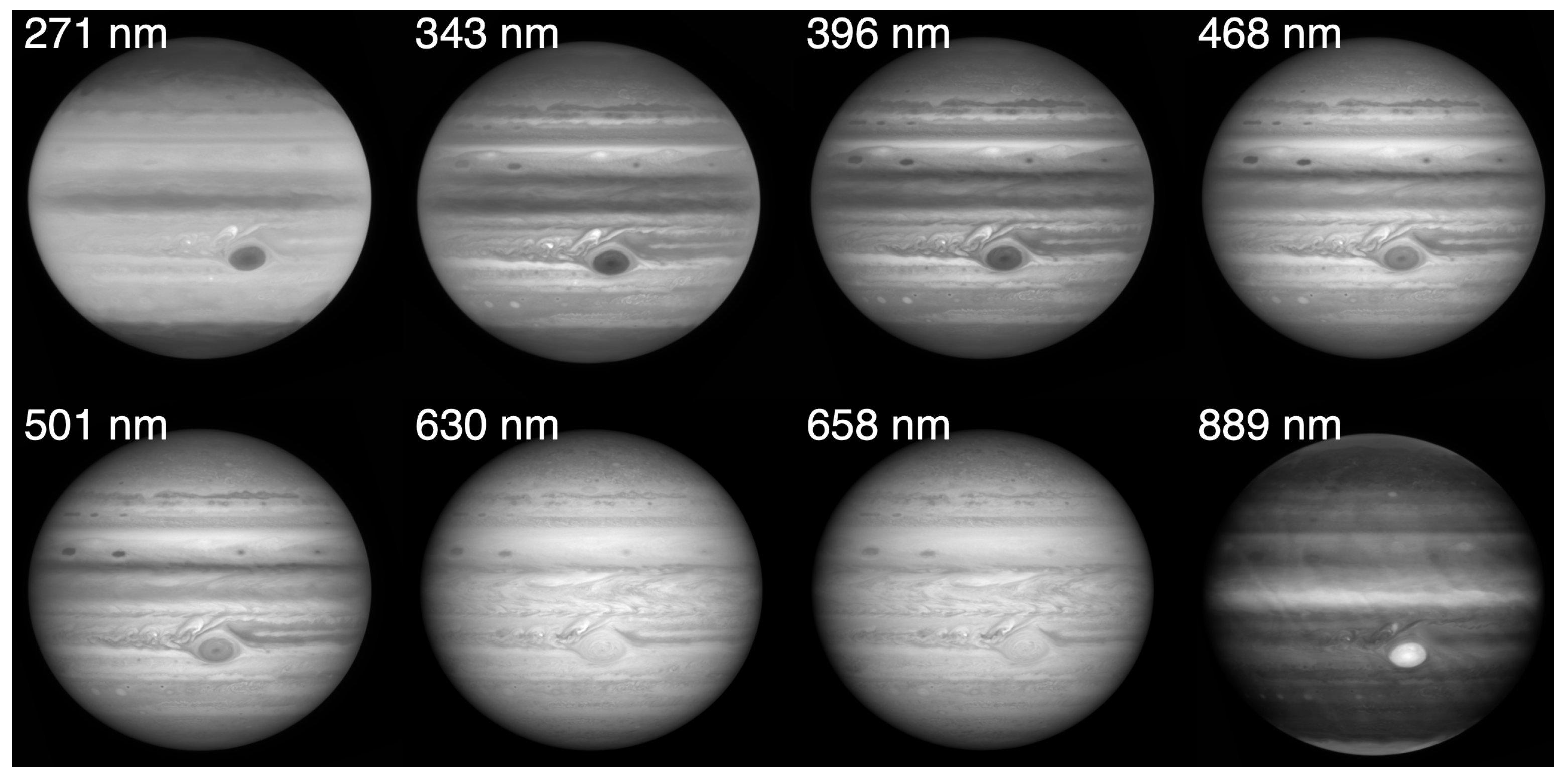
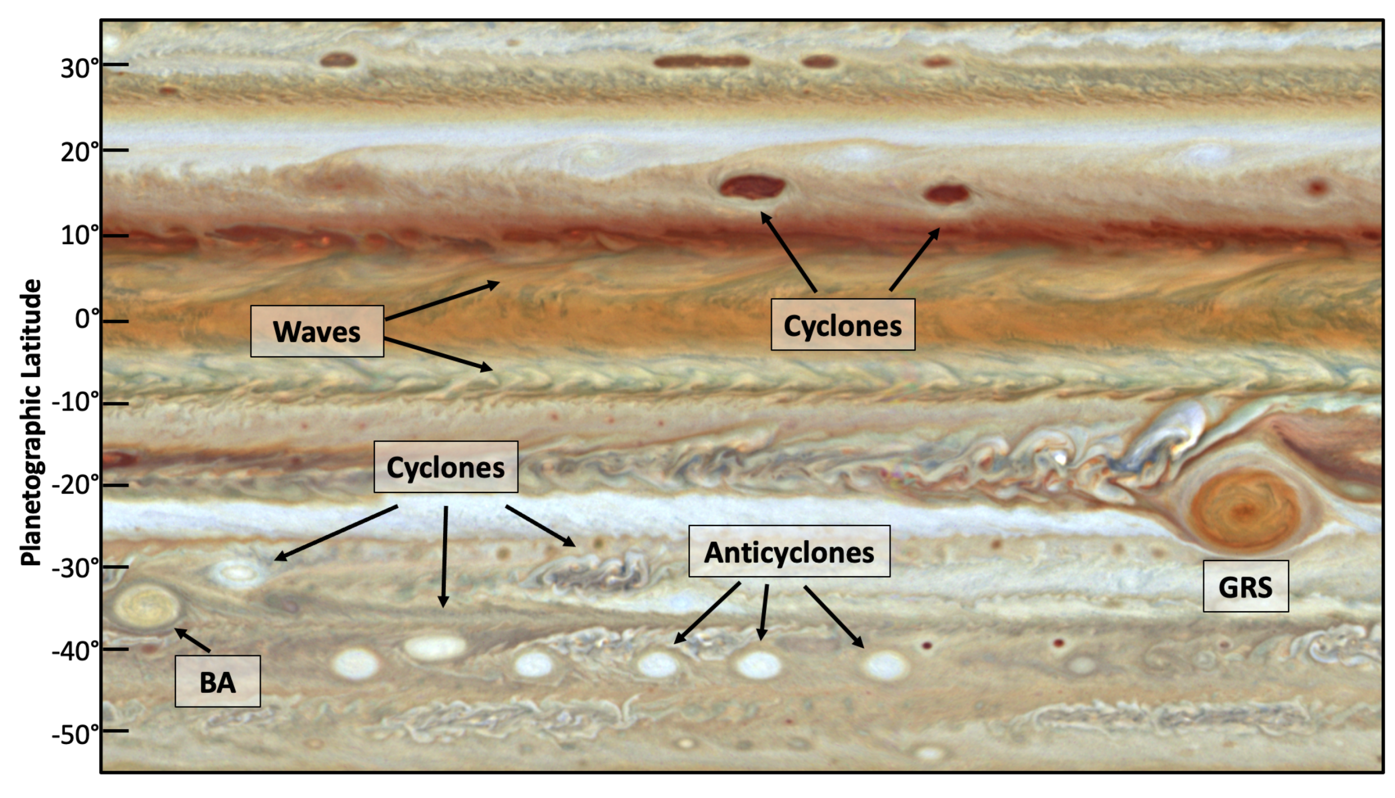
3.1. Jupiter
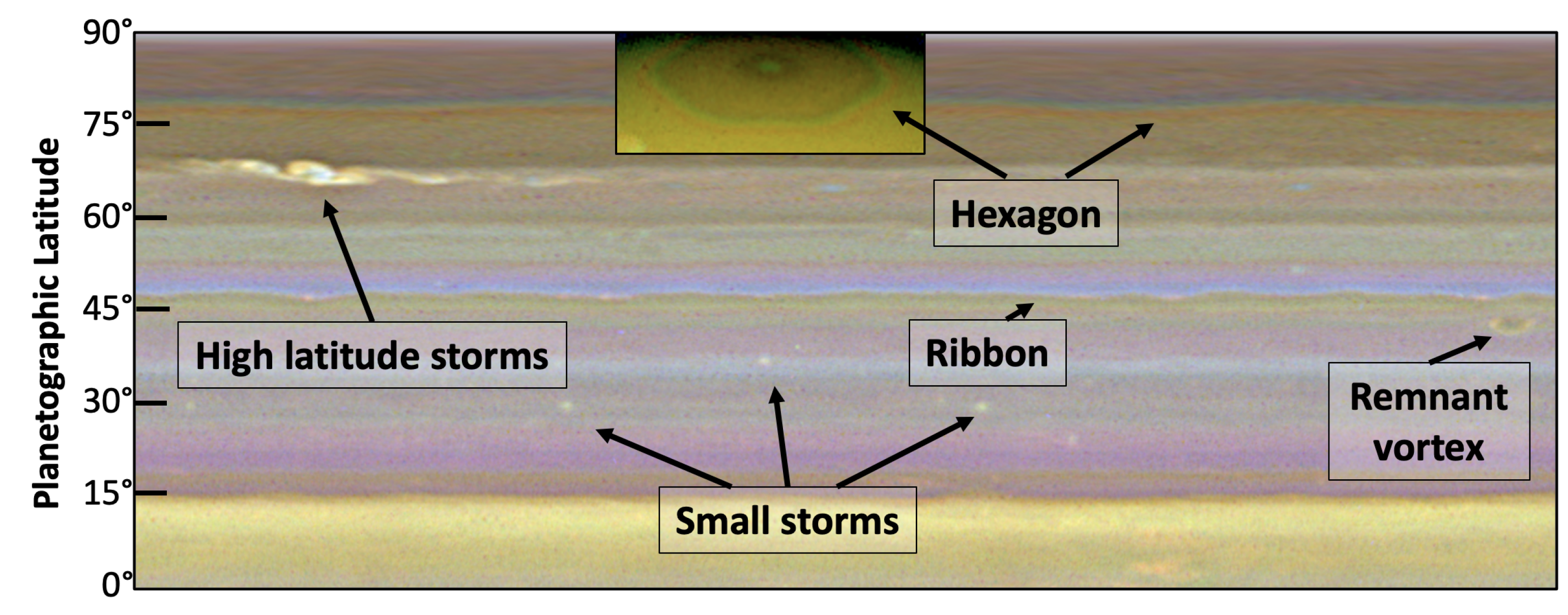
3.2. Saturn
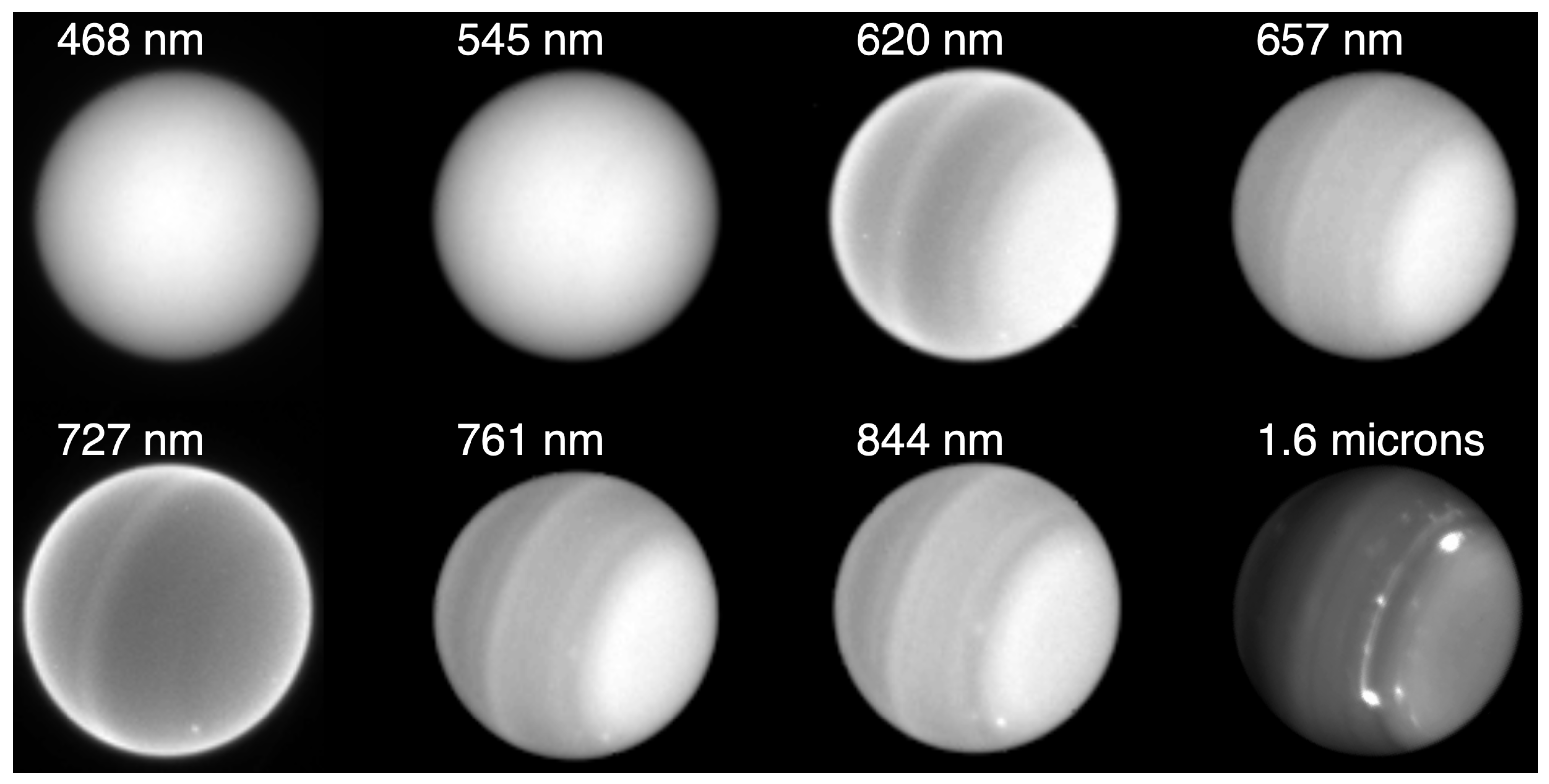
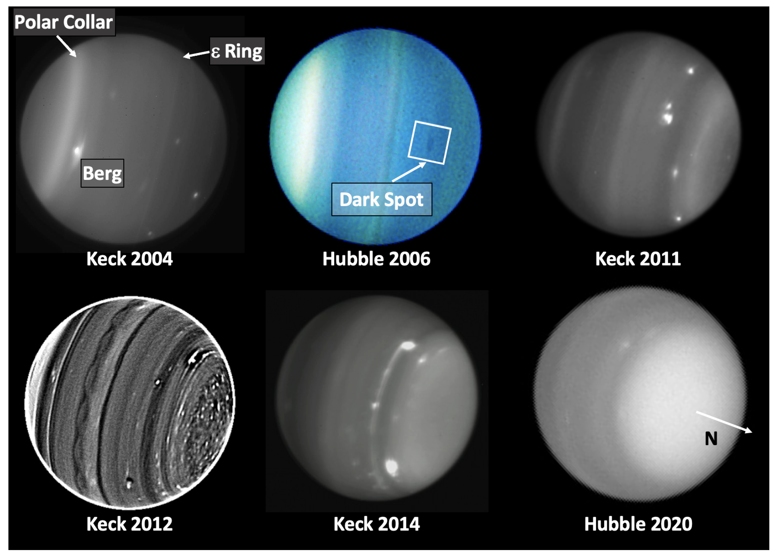
3.3. Uranus
3.4. Neptune

4. Dynamics and Cloud Variability
4.1. Zonal Winds
4.2. Waves
4.3. Vertical Cloud Structure
5. Discussion

| Planet | Orbital | Orbital | Orbital | Axial | 2/ | 2/ |
|---|---|---|---|---|---|---|
| Period | Inclination | Eccentricity | Tilt | at 0.1 bar | at 1 bar | |
| Jupiter | 11.9 years | 1.3 | 0.049 | 3.1 | 1 | 0.2 |
| Saturn | 29.5 years | 2.5 | 0.052 | 26.7 | 1 | 0.3 |
| Uranus | 84.0 years | 0.8 | 0.047 | 97.8 | 3 | 0.7 |
| Neptune | 164.8 years | 1.8 | 0.010 | 28.3 | 2 | 0.3 |
6. Summary
Author Contributions
Funding
Institutional Review Board Statement
Informed Consent Statement
Data Availability Statement
Acknowledgments
Conflicts of Interest
References
- Peek, B. The Planet Jupiter; Faber and Faber: London, UK, 1958. [Google Scholar]
- Rogers, J. The Giant Planet Jupiter; Cambridge University Press: Cambridge, UK, 1995. [Google Scholar]
- Chapman, C.R. Jupiter’s Zonal Winds: Variation with Latitude. J. Atmos. Sci. 1969, 26, 986–990. [Google Scholar] [CrossRef]
- Hide, R. Jupiter and Saturn. Proc. R. Soc. Lond. Ser. Math. Phys. Sci. 1974, 336, 63–84. [Google Scholar]
- Peebles, P. The Structure and Composition of Jupiter and Saturn. Astrophys. J. 1964, 140, 328. [Google Scholar] [CrossRef]
- Owen, T. The spectra of Jupiter and Saturn in the photographic infrared. Icarus 1969, 10, 355–364. [Google Scholar] [CrossRef]
- Hubbard, W. Thermal Models of Jupiter and Saturn. Astrophys. J. 1969, 155, 333. [Google Scholar] [CrossRef]
- Smith, B.A.; Soderblom, L.A.; Johnson, T.V.; Ingersoll, A.P.; Collins, S.A.; Shoemaker, E.M.; Hunt, G.E.; Masursky, H.; Carr, M.H.; Davies, M.E.; et al. The Jupiter System Through the Eyes of Voyager 1. Science 1979, 204, 951–972. [Google Scholar] [CrossRef]
- Smith, B.A.; Soderblom, L.A.; Beebe, R.; Boyce, J.; Briggs, G.; Carr, M.; Collins, S.A.; Cook, A.F.; Danielson, G.E.; Davies, M.E.; et al. The Galilean Satellites and Jupiter: Voyager 2 Imaging Science Results. Science 1979, 206, 927–950. [Google Scholar] [CrossRef]
- Smith, B.A.; Soderblom, L.; Beebe, R.; Boyce, J.; Briggs, G.; Bunker, A.; Collins, S.A.; Hansen, C.J.; Johnson, T.V.; Mitchell, J.L.; et al. Encounter with Saturn: Voyager 1 Imaging Science Results. Science 1981, 212, 163–191. [Google Scholar] [CrossRef]
- Smith, B.A.; Soderblom, L.; Batson, R.; Bridges, P.; Inge, J.; Masursky, H.; Shoemaker, E.; Beebe, R.; Boyce, J.; Briggs, G.; et al. A New Look at the Saturn System: The Voyager 2 Images. Science 1982, 215, 504–537. [Google Scholar] [CrossRef]
- Smith, B.; Soderblom, L.; Beebe, R.; Bliss, D.; Boyce, J.; Brahic, A.; Briggs, G.; Brown, R.; Collins, S.; Cook, A.; et al. Voyager 2 in the Uranian System: Imaging Science Results. Science 1986, 233, 43–64. [Google Scholar] [CrossRef]
- Smith, B.A.; Soderblom, L.A.; Banfield, D.; Barnet, C.; Basilevsky, A.T.; Beebe, R.F.; Bollinger, K.; Boyce, J.M.; Brahic, A.; Briggs, G.A.; et al. Voyager 2 at Neptune: Imaging Science Results. Science 1989, 246, 1422–1449. [Google Scholar] [CrossRef] [PubMed]
- García-Melendo, E.; Arregi, J.; Rojas, J.; Hueso, R.; Barrado-Izagirre, N.; Gómez-Forrellad, J.; Pérez-Hoyos, S.; Sanz-Requena, J.; Sánchez-Lavega, A. Dynamics of Jupiter’s equatorial region at cloud top level from Cassini and HST images. Icarus 2011, 211, 1242–1257. [Google Scholar] [CrossRef]
- Wong, M.H.; Simon, A.A.; Tollefson, J.W.; de Pater, I.; Barnett, M.N.; Hsu, A.I.; Stephens, A.W.; Orton, G.S.; Fleming, S.W.; Goullaud, C.; et al. High-resolution UV/Optical/IR Imaging of Jupiter in 2016–2019. Astrophys. J. Suppl. 2020, 247, 58. [Google Scholar] [CrossRef]
- Simon, A.A.; Wong, M.H.; Orton, G.S. First Results from the Hubble OPAL Program: Jupiter in 2015. Astrophys. J. 2015, 812, 55. [Google Scholar] [CrossRef]
- Beckers, J.M. Adaptive Optics for Astronomy: Principles, Performance, and Applications. Annu. Rev. Astron. Astrophys. 1993, 31, 13–62. [Google Scholar] [CrossRef]
- Rigaut, F. Astronomical Adaptive Optics. Publ. Astron. Soc. Pac. 2015, 127, 1197–1203. [Google Scholar] [CrossRef]
- de Pater, I.; Fletcher, L.N.; Pérez-Hoyos, S.; Hammel, H.B.; Orton, G.S.; Wong, M.H.; Luszcz-Cook, S.; Sánchez-Lavega, A.; Boslough, M. A multi-wavelength study of the 2009 impact on Jupiter: Comparison of high resolution images from Gemini, Keck and HST. Icarus 2010, 210, 722–741. [Google Scholar] [CrossRef]
- de Pater, I.; Wong, M.H.; Marcus, P.; Luszcz-Cook, S.; Ádámkovics, M.; Conrad, A.; Asay-Davis, X.; Go, C. Persistent rings in and around Jupiter’s anticyclones—Observations and theory. Icarus 2010, 210, 742–762. [Google Scholar] [CrossRef]
- de Pater, I.; Wong, M.H.; de Kleer, K.; Hammel, H.B.; Ádámkovics, M.; Conrad, A. Keck adaptive optics images of Jupiter’s north polar cap and Northern Red Oval. Icarus 2011, 213, 559–563. [Google Scholar] [CrossRef]
- Hueso, R.; de Pater, I.; Simon, A.; Sánchez-Lavega, A.; Delcroix, M.; Wong, M.H.; Tollefson, J.W.; Baranec, C.; de Kleer, K.; Luszcz-Cook, S.H.; et al. Neptune long-lived atmospheric features in 2013–2015 from small (28-cm) to large (10-m) telescopes. Icarus 2017, 295, 89–109. [Google Scholar] [CrossRef]
- Hammel, H.B.; Sitko, M.L.; Lynch, D.K.; Orton, G.S.; Russell, R.W.; Geballe, T.R.; de Pater, I. Distribution of Ethane and Methane Emission on Neptune. Astron. J. 2007, 134, 637–641. [Google Scholar] [CrossRef]
- Sromovsky, L.A.; de Pater, I.; Fry, P.M.; Hammel, H.B.; Marcus, P. High S/N Keck and Gemini AO imaging of Uranus during 2012–2014: New cloud patterns, increasing activity, and improved wind measurements. Icarus 2015, 258, 192–223. [Google Scholar] [CrossRef]
- de Pater, I.; Sromovsky, L.A.; Fry, P.M.; Hammel, H.B.; Baranec, C.; Sayanagi, K.M. Record-breaking storm activity on Uranus in 2014. Icarus 2015, 252, 121–128. [Google Scholar] [CrossRef]
- Sromovsky, L.A.; Fry, P.M. The methane abundance and structure of Uranus’ cloud bands inferred from spatially resolved 2006 Keck grism spectra. Icarus 2008, 193, 252–266. [Google Scholar] [CrossRef]
- Sromovsky, L.A.; Fry, P.M. Spatially resolved cloud structure on Uranus: Implications of near-IR adaptive optics imaging. Icarus 2007, 192, 527–557. [Google Scholar] [CrossRef]
- Sromovsky, L.A.; Fry, P.M.; Hammel, H.B.; de Pater, I.; Rages, K.A.; Showalter, M.R. Dynamics, evolution, and structure of Uranus’ brightest cloud feature. Icarus 2007, 192, 558–575. [Google Scholar] [CrossRef]
- Sromovsky, L.A.; Fry, P.M. Dynamics of cloud features on Uranus. Icarus 2005, 179, 459–484. [Google Scholar] [CrossRef]
- Hammel, H.B.; de Pater, I.; Gibbard, S.G.; Lockwood, G.W.; Rages, K. New cloud activity on Uranus in 2004: First detection of a southern feature at 2.2 micron. Icarus 2005, 175, 284–288. [Google Scholar] [CrossRef]
- Gibbard, S.G.; de Pater, I.; Hammel, H.B. Near-infrared adaptive optics imaging of the satellites and individual rings of Uranus. Icarus 2005, 174, 253–262. [Google Scholar] [CrossRef]
- de Pater, I.; Gibbard, S.G.; Macintosh, B.A.; Roe, H.G.; Gavel, D.T.; Max, C.E. Keck Adaptive Optics Images of Uranus and Its Rings. Icarus 2002, 160, 359–374. [Google Scholar] [CrossRef]
- Hammel, H.B.; Rages, K.; Lockwood, G.W.; Karkoschka, E.; de Pater, I. New Measurements of the Winds of Uranus. Icarus 2001, 153, 229–235. [Google Scholar] [CrossRef]
- Tollefson, J.; de Pater, I.; Marcus, P.S.; Luszcz-Cook, S.; Sromovsky, L.A.; Fry, P.M.; Fletcher, L.N.; Wong, M.H. Vertical wind shear in Neptune’s upper atmosphere explained with a modified thermal wind equation. Icarus 2018, 311, 317–339. [Google Scholar] [CrossRef]
- de Pater, I.; Fletcher, L.N.; Luszcz-Cook, S.; DeBoer, D.; Butler, B.; Hammel, H.B.; Sitko, M.L.; Orton, G.; Marcus, P.S. Neptune’s global circulation deduced from multi-wavelength observations. Icarus 2014, 237, 211–238. [Google Scholar] [CrossRef]
- Fitzpatrick, P.J.; de Pater, I.; Luszcz-Cook, S.; Wong, M.H.; Hammel, H.B. Dispersion in Neptune’s zonal wind velocities from NIR Keck AO observations in July 2009. Astrophys. Space Sci. 2014, 350, 65–88. [Google Scholar] [CrossRef]
- Martin, S.C.; de Pater, I.; Marcus, P. Neptune’s zonal winds from near-IR Keck adaptive optics imaging in August 2001. Astrophys. Space Sci. 2012, 337, 65–78. [Google Scholar] [CrossRef]
- Fry, P.M.; Sromovsky, L.A. Keck NIRC2 photometry of Uranus, uranian satellites, and Triton in August 2004. Icarus 2007, 192, 117–134. [Google Scholar] [CrossRef]
- Gibbard, S.G.; de Pater, I.; Roe, H.G.; Martin, S.; Macintosh, B.A.; Max, C.E. The altitude of Neptune cloud features from high-spatial-resolution near-infrared spectra. Icarus 2003, 166, 359–374. [Google Scholar] [CrossRef]
- Max, C.E.; Macintosh, B.A.; Gibbard, S.G.; Gavel, D.T.; Roe, H.G.; de Pater, I.; Ghez, A.M.; Acton, D.S.; Lai, O.; Stomski, P.; et al. Cloud Structures on Neptune Observed with Keck Telescope Adaptive Optics. Astron. J. 2003, 125, 364–375. [Google Scholar] [CrossRef]
- Wizinowich, P.; Acton, D.S.; Shelton, C.; Stomski, P.; Gathright, J.; Ho, K.; Lupton, W.; Tsubota, K.; Lai, O.; Max, C.; et al. First Light Adaptive Optics Images from the Keck II Telescope: A New Era of High Angular Resolution Imagery. Pub. Astro. Soc. Pac. 2000, 112, 315–319. [Google Scholar] [CrossRef]
- Uno, T.; Kasaba, Y.; Tao, C.; Sakanoi, T.; Kagitani, M.; Fujisawa, S.; Kita, H.; Badman, S.V. Vertical emissivity profiles of Jupiter’s northern H3+ and H2 infrared auroras observed by Subaru/IRCS. J. Geophys. Res. (Space Phys.) 2014, 119, 10219–10241. [Google Scholar] [CrossRef]
- Kita, H.; Fujisawa, S.; Tao, C.; Kagitani, M.; Sakanoi, T.; Kasaba, Y. Horizontal and vertical structures of Jovian infrared aurora: Observation using Subaru IRCS with adaptive optics. Icarus 2018, 313, 93–106. [Google Scholar] [CrossRef]
- Watanabe, H.; Kita, H.; Tao, C.; Kagitani, M.; Sakanoi, T.; Kasaba, Y. Pulsation Characteristics of Jovian Infrared Northern Aurora Observed by the Subaru IRCS with Adaptive Optics. Geophys. Res. Lett. 2018, 45, 11547–11554. [Google Scholar] [CrossRef]
- Wong, M.H.; Marchis, F.; Marchetti, E.; Amico, P.; Tordo, S.; Bouy, H.; de Pater, I. A shift in Jupiter’s equatorial haze distribution imaged with the Multi-Conjugate Adaptive Optics Demonstrator at the VLT. arXiv 2008, arXiv:0810.3703. [Google Scholar]
- Chowdhury, M.N.; Stallard, T.S.; Melin, H.; Johnson, R.E. Exploring Key Characteristics in Saturn’s Infrared Auroral Emissions Using VLT-CRIRES: H3+ Intensities, Ion Line-of-Sight Velocities, and Rotational Temperatures. Geophys. Res. Lett. 2019, 46, 7137–7146. [Google Scholar] [CrossRef]
- Irwin, P.G.J.; Fletcher, L.N.; Read, P.L.; Tice, D.; de Pater, I.; Orton, G.S.; Teanby, N.A.; Davis, G.R. Spectral analysis of Uranus’ 2014 bright storm with VLT/SINFONI. Icarus 2016, 264, 72–89. [Google Scholar] [CrossRef]
- Irwin, P.G.J.; Wong, M.H.; Simon, A.A.; Orton, G.S.; Toledo, D. HST/WFC3 observations of Uranus’ 2014 storm clouds and comparison with VLT/SINFONI and IRTF/Spex observations. Icarus 2017, 288, 99–119. [Google Scholar] [CrossRef]
- Braude, A.S.; Irwin, P.G.; Orton, G.S.; Fletcher, L.N. Colour and tropospheric cloud structure of Jupiter from MUSE/VLT: Retrieving a universal chromophore. Icarus 2020, 338, 113589. [Google Scholar] [CrossRef]
- Irwin, P.G.J.; Dobinson, J.; James, A.; Toledo, D.; Teanby, N.A.; Fletcher, L.N.; Orton, G.S.; Pérez-Hoyos, S. Latitudinal variation of methane mole fraction above clouds in Neptune’s atmosphere from VLT/MUSE-NFM: Limb-darkening reanalysis. Icarus 2021, 357, 114277. [Google Scholar] [CrossRef]
- Irwin, P.G.J.; Toledo, D.; Braude, A.S.; Bacon, R.; Weilbacher, P.M.; Teanby, N.A.; Fletcher, L.N.; Orton, G.S. Latitudinal variation in the abundance of methane (CH4) above the clouds in Neptune’s atmosphere from VLT/MUSE Narrow Field Mode Observations. Icarus 2019, 331, 69–82. [Google Scholar] [CrossRef]
- Irwin, P.G.J.; Teanby, N.A.; Davis, G.R.; Fletcher, L.N.; Orton, G.S.; Calcutt, S.B.; Tice, D.S.; Hurley, J. Further seasonal changes in Uranus’s cloud structure observed by Gemini-North and UKIRT. Icarus 2012, 218, 47–55. [Google Scholar] [CrossRef]
- Irwin, P.G.J.; Teanby, N.A.; Davis, G.R.; Fletcher, L.N.; Orton, G.S.; Tice, D.; Kyffin, A. Uranus’s cloud structure and seasonal variability from Gemini-North and UKIRT observations. Icarus 2011, 212, 339–350. [Google Scholar] [CrossRef]
- Irwin, P.G.J.; Teanby, N.A.; Davis, G.R.; Fletcher, L.N.; Orton, G.S.; Tice, D.; Hurley, J.; Calcutt, S.B. Multispectral imaging observations of Neptune’s cloud structure with Gemini-North. Icarus 2011, 216, 141–158. [Google Scholar] [CrossRef]
- Giles, R.S.; Orton, G.S.; Stephens, A.W.; Wong, M.H.; Irwin, P.G.J.; Sinclair, J.A.; Tabataba-Vakili, F. Wave Activity in Jupiter’s North Equatorial Belt From Near-Infrared Reflectivity Observations. Geophys. Res. Lett. 2019, 46, 1232–1241. [Google Scholar] [CrossRef]
- Roman, M.T.; Banfield, D.; Gierasch, P.J. Aerosols and methane in the ice giant atmospheres inferred from spatially resolved, near-infrared spectra: I. Uranus, 2001–2007. Icarus 2018, 310, 54–76. [Google Scholar] [CrossRef]
- Roddier, F.; Roddier, C.; Graves, J.E.; Northcott, M.J.; Owen, T. NOTE: Neptune’s Cloud Structure and Activity: Ground-Based Monitoring with Adaptive Optics. Icarus 1998, 136, 168–172. [Google Scholar] [CrossRef]
- Roddier, F.; Roddier, C.; Brahic, A.; Dumas, C.; Graves, J.E.; Northcott, M.J.; Owen, T. First ground-based adaptive optics observations of Neptune and Proteus. Planet. Space Sci. 1997, 45, 1031–1036. [Google Scholar] [CrossRef]
- Roe, H.G.; Gavel, D.; Max, C.; de Pater, I.; Gibbard, S.; Macintosh, B.; Baines, K.H. Near-Infrared Observations of Neptune’s Tropospheric Cloud Layer with the Lick Observatory Adaptive Optics System. Astron. J. 2001, 122, 1636–1643. [Google Scholar] [CrossRef]
- Glenar, D.A.; Hillman, J.J.; Lelouarn, M.; Fugate, R.; Drummond, J.D. Multispectral Imagery of Jupiter and Saturn Using Adaptive Optics and Acousto-Optic Tuning. Pub. Astron. Soc. Pac. 1997, 109, 326–337. [Google Scholar] [CrossRef]
- Sromovsky, L.A. Latitudinal and Longitudinal Oscillations of Cloud Features on Neptune. Science 1991, 254, 684–686. [Google Scholar] [CrossRef]
- Trigo-Rodriguez, J.; Sánchez-Lavega, A.; Gómez, J.; Lecacheux, J.; Colas, F.; Miyazaki, I. The 90-day oscillations of Jupiter’s Great Red Spot revisited. Planet. Space Sci. 2000, 48, 331–339. [Google Scholar] [CrossRef]
- Simon, A.A.; Tabataba-Vakili, F.; Cosentino, R.; Beebe, R.F.; Wong, M.H.; Orton, G.S. Historical and Contemporary Trends in the Size, Drift, and Color of Jupiter’s Great Red Spot. Astron. J. 2018, 155, 151. [Google Scholar] [CrossRef]
- Morales-Juberías, R.; Simon, A.A.; Cosentino, R.G. Analysis of the long-term drift rates and oscillations of Jupiter’s largest vortices. Icarus 2022, 372, 114732. [Google Scholar] [CrossRef]
- Wong, M.H.; Marcus, P.S.; Simon, A.A.; de Pater, I.; Tollefson, J.W.; Asay-Davis, X. Evolution of the Horizontal Winds in Jupiter’s Great Red Spot From One Jovian Year of HST/WFC3 Maps. Geophys. Res. Lett. 2021, 48, e2021GL093982. [Google Scholar] [CrossRef]
- Hammel, H.B.; Wong, M.H.; Clarke, J.T.; de Pater, I.; Fletcher, L.N.; Hueso, R.; Noll, K.; Orton, G.S.; Pérez-Hoyos, S.; Sánchez-Lavega, A.; et al. Jupiter after the 2009 Impact: Hubble Space Telescope Imaging of the Impact-Generated Debris and its Temporal Evolution. Astrophys. J. 2010, 715, L150–L154. [Google Scholar] [CrossRef]
- Hsu, A.I.; Wong, M.H.; Simon, A.A. Lifetimes and Occurrence Rates of Dark Vortices on Neptune from 25 Years of Hubble Space Telescope Images. Astron. J. 2019, 157, 152. [Google Scholar] [CrossRef]
- Hammel, H.B.; Lockwood, G.W.; Mills, J.R.; Barnet, C.D. Hubble Space Telescope Imaging of Neptune’s Cloud Structure in 1994. Science 1995, 268, 1740–1742. [Google Scholar] [CrossRef]
- Sromovsky, L.; Hammel, H.; de Pater, I.; Fry, P.; Rages, K.; Showalter, M.; Merline, W.; Tamblyn, P.; Neyman, C.; Margot, J.L.; et al. Episodic bright and dark spots on Uranus. Icarus 2012, 220, 6–22. [Google Scholar] [CrossRef]
- Sromovsky, L.; Fry, P.; Dowling, T.; Baines, K.; Limaye, S. Neptune’s Atmospheric Circulation and Cloud Morphology: Changes Revealed by 1998 HST Imaging. Icarus 2001, 150, 244–260. [Google Scholar] [CrossRef]
- Atreya, S.K.; Romani, P.N. Photochemistry and clouds of Jupiter, Saturn and Uranus. In Recent Advances in Planetary Meteorology; Hunt, G.E., Ed.; Cambridge University Press: Cambridge, UK, 1985; pp. 17–68. [Google Scholar]
- West, R.A.; Strobel, D.F.; Tomasko, M.G. Clouds, aerosols, and photochemistry in the Jovian atmosphere. Icarus 1986, 65, 161–217. [Google Scholar] [CrossRef]
- Lindal, G.F. The Atmosphere of Neptune: An Analysis of Radio Occultation Data Acquired with Voyager 2. Astron. J. 1992, 103, 967. [Google Scholar] [CrossRef]
- Schaller, E.L.; Roe, H.G.; Schneider, T.; Brown, M.E. Storms in the tropics of Titan. Nature 2009, 460, 873–875. [Google Scholar] [CrossRef]
- Fletcher, L.N.; Orton, G.; Rogers, J.; Giles, R.; Payne, A.; Irwin, P.; Vedovato, M. Moist convection and the 2010–2011 revival of Jupiter’s South Equatorial Belt. Icarus 2017, 286, 94–117. [Google Scholar] [CrossRef]
- Simon, A.A.; Sanchez-Lavega, A.; Legarreta, J.; Sanz-Requena, J.F.; Perez-Hoyos, S.; Garcia-Melendo, E.; Carlson, R.W. Spectral comparison and stability of red regions on Jupiter. J. Geophys. Res. Planets 2015, 120, 483–494. [Google Scholar] [CrossRef]
- Loeffler, M.J.; Hudson, R.L.; Chanover, N.J.; Simon, A.A. The spectrum of Jupiter’s Great Red Spot: The case for ammonium hydrosulfide (NH4SH). Icarus 2016, 271, 265–268. [Google Scholar] [CrossRef]
- Carlson, R.; Baines, K.; Anderson, M.; Filacchione, G.; Simon, A. Chromophores from photolyzed ammonia reacting with acetylene: Application to Jupiter’s Great Red Spot. Icarus 2016, 274, 106–115. [Google Scholar] [CrossRef]
- Sromovsky, L.; Baines, K.; Fry, P.; Carlson, R. A possibly universal red chromophore for modeling color variations on Jupiter. Icarus 2017, 291, 232–244. [Google Scholar] [CrossRef]
- Weidenschilling, S.; Lewis, J. Atmospheric and cloud structures of the Jovian planets. Icarus 1973, 20, 465–476. [Google Scholar] [CrossRef]
- Atreya, S.K. Atmospheres and Ionospheres of the Outer Planets and Their Satellites; Springer: London, UK, 1986; p. 90. [Google Scholar]
- Baines, K.H.; Carlson, R.W.; Kamp, L.W. Fresh Ammonia Ice Clouds in Jupiter. I. Spectroscopic Identification, Spatial Distribution, and Dynamical Implications. Icarus 2002, 159, 74–94. [Google Scholar] [CrossRef]
- Simon-Miller, A.A.; Conrath, B.; Gierasch, P.J.; Beebe, R.F. A Detection of Water Ice on Jupiter with Voyager IRIS. Icarus 2000, 145, 454–461. [Google Scholar] [CrossRef]
- Simon-Miller, A.A.; Gierasch, P.J.; Beebe, R.F.; Conrath, B.; Flasar, F.; Achterberg, R.K. New Observational Results Concerning Jupiter’s Great Red Spot. Icarus 2002, 158, 249–266. [Google Scholar] [CrossRef]
- Beebe, R. Jupiter The Giant Planet; Smithsonian: Washington, DC, USA, 1994. [Google Scholar]
- Sánchez-Lavega, A.; Anguiano-Arteaga, A.; Iñurrigarro, P.; Garcia-Melendo, E.; Legarreta, J.; Hueso, R.; Sanz-Requena, J.F.; Pérez-Hoyos, S.; Mendikoa, I.; Soria, M.; et al. Jupiter’s Great Red Spot: Strong Interactions With Incoming Anticyclones in 2019. J. Geophys. Res. Planets 2021, 126, e2020JE006686. [Google Scholar] [CrossRef]
- Sanchez-Lavega, A.; Orton, G.; Morales, R.; Lecacheux, J.; Colas, F.; Fisher, B.; Fukumura-Sawada, P.; Golisch, W.; Griep, D.; Kaminski, C.; et al. The Merger of Two Giant Anticyclones in the Atmosphere of Jupiter. Icarus 2001, 149, 491–495. [Google Scholar] [CrossRef]
- Youssef, A.; Marcus, P.S. The dynamics of jovian white ovals from formation to merger. Icarus 2003, 162, 74–93. [Google Scholar] [CrossRef]
- Simon-Miller, A.A.; Chanover, N.J.; Orton, G.S.; Sussman, M.; Tsavaris, I.G.; Karkoschka, E. Jupiter’s White Oval turns red. Icarus 2006, 185, 558–562. [Google Scholar] [CrossRef]
- DelGenio, A.D.; Achterberg, R.K.; Baines, K.H.; Flasar, F.M.; Read, P.L.; Sánchez-Lavega, A.; Showman, A.P. Saturn Atmospheric Structure and Dynamics. In Saturn from Cassini-Huygens; Dougherty, M.K., Esposito, L.W., Krimigis, S.M., Eds.; Springer: Dordrecht, The Netherlands, 2009; pp. 113–159. [Google Scholar] [CrossRef]
- Fletcher, L.N.; Greathouse, T.K.; Guerlet, S.; Moses, J.I.; West, R.A. Saturn’s Seasonally Changing Atmosphere: Thermal Structure, Composition and Aerosols. In Saturn in the 21st Century; Baines, K.H., Flasar, F.M., Krupp, N., Stallard, T., Eds.; Cambridge Planetary Science, Cambridge University Press: Cambridge, UK, 2018; pp. 251–294. [Google Scholar] [CrossRef]
- Sromovsky, L.; Baines, K.; Fry, P. Evolution of Saturn’s north polar color and cloud structure between 2012 and 2017 inferred from Cassini VIMS and ISS observations. Icarus 2021, 362, 114409. [Google Scholar] [CrossRef]
- Gunnarson, J.L.; Sayanagi, K.M.; Blalock, J.J.; Fletcher, L.N.; Ingersoll, A.P.; Dyudina, U.A.; Ewald, S.P.; Draham, R.L. Saturn’s New Ribbons: Cassini Observations of Planetary Waves in Saturn’s 42N Atmospheric Jet. Geophys. Res. Lett. 2018, 45, 7399–7408. [Google Scholar] [CrossRef]
- Simon, A.; Hueso, R.; Sanchez-Lavega, A.; Wong, M.H. Midsummer Atmospheric Changes in Saturn’s Northern Hemisphere from the Hubble OPAL Program. Planet. Sci. J. 2021, 2, 47. [Google Scholar] [CrossRef]
- Sánchez-Lavega, A.; del Río-Gaztelurrutia, T.; Delcroix, M.; Legarreta, J.J.; Gómez-Forrellad, J.M.; Hueso, R.; García-Melendo, E.; Pérez-Hoyos, S.; Barrado-Navascués, D.; Lillo, J.; et al. Ground-based observations of the long-term evolution and death of Saturn’s 2010 Great White Spot. Icarus 2012, 220, 561–576. [Google Scholar] [CrossRef]
- del Río-Gaztelurrutia, T.; Sánchez-Lavega, A.; Antuñano, A.; Legarreta, J.; García-Melendo, E.; Sayanagi, K.M.; Hueso, R.; Wong, M.H.; Pérez-Hoyos, S.; Rojas, J.F.; et al. A planetary-scale disturbance in a long living three vortex coupled system in Saturn’s atmosphere. Icarus 2018, 302, 499–513. [Google Scholar] [CrossRef]
- Godfrey, D. A Hexagonal feature around Saturn’s north pole. Icarus 1988, 76, 335–356. [Google Scholar] [CrossRef]
- Barbosa Aguiar, A.; Read, P.; Wordsworth, R.; Salter, T.; Yamazaki, Y. A laboratory model of Saturn’s North Polar Hexagon. Icarus 2010, 206, 755–763. [Google Scholar] [CrossRef]
- Morales-Juberias, R.; Sayanagi, K.; Simon, A.; Fletcher, L.; Cosentino, R. Meandering Shallow Atmospheric Jet as a Model of Saturn’ North-Polar Hexagon. Astrophys. J. Lett. 2015, 806, L18. [Google Scholar] [CrossRef]
- Fletcher, L.N.; Orton, G.S.; Sinclair, J.A.; Guerlet, S.; Read, P.L.; Antuñano, A.; Achterberg, R.K.; Flasar, F.M.; Irwin, P.G.J.; Bjoraker, G.L.; et al. A hexagon in Saturn’s northern stratosphere surrounding the emerging summertime polar vortex. Nat. Commun. 2018, 9, 3564. [Google Scholar] [CrossRef] [PubMed]
- Sromovsky, L.A.; Revercomb, H.E.; Krauss, R.J.; Suomi, V.E. Voyager 2 Observations of Saturn’s Northern Mid-Latitude Cloud Features: Morphology, Motions, and Evolution. J. Geophys. Res. 1983, 88, 8650–8666. [Google Scholar] [CrossRef]
- Sayanagi, K.M.; Morales-Juberías, R.; Ingersoll, A.P. Saturn’s Northern Hemisphere Ribbon: Simulations and Comparison with the Meandering Gulf Stream. J. Atmos. Sci. 2010. [Google Scholar] [CrossRef]
- Cosentino, R.G.; Simon, A.; Morales-Juberias, R.; Sayanagi, K.M. Observations and Numerical Modeling of the Jovian Ribbon. Astrophys. J. 2015, 810, L10. [Google Scholar] [CrossRef]
- Karkoschka, E. Clouds of High Contrast on Uranus. Science 1998, 280, 570. [Google Scholar] [CrossRef]
- Karkoschka, E. Uranus’ southern circulation revealed by Voyager 2: Unique characteristics. Icarus 2015, 250, 294–307. [Google Scholar] [CrossRef]
- Sromovsky, L.A.; Karkoschka, E.; Fry, P.M.; de Pater, I.; Hammel, H.B. The methane distribution and polar brightening on Uranus based on HST/STIS, Keck/NIRC2, and IRTF/SpeX observations through 2015. Icarus 2019, 317, 266–306. [Google Scholar] [CrossRef]
- Fletcher, L.N. The Atmosphere of Uranus. arXiv 2021, arXiv:2105.06377. [Google Scholar]
- Sromovsky, L.A.; Karkoschka, E.; Fry, P.M.; Hammel, H.B.; de Pater, I.; Rages, K. Methane depletion in both polar regions of Uranus inferred from HST/STIS and Keck/NIRC2 observations. Icarus 2014, 238, 137–155. [Google Scholar] [CrossRef]
- Karkoschka, E.; Tomasko, M. The haze and methane distributions on Uranus from HST-STIS spectroscopy. Icarus 2009, 202, 287–309. [Google Scholar] [CrossRef]
- Toledo, D.; Irwin, P.G.; Rannou, P.; Teanby, N.A.; Simon, A.A.; Wong, M.H.; Orton, G.S. Constraints on Uranus’s haze structure, formation and transport. Icarus 2019, 333, 1–11. [Google Scholar] [CrossRef]
- Hammel, H.; Sromovsky, L.; Fry, P.; Rages, K.; Showalter, M.; de Pater, I.; van Dam, M.; LeBeau, R.; Deng, X. The Dark Spot in the atmosphere of Uranus in 2006: Discovery, description, and dynamical simulations. Icarus 2009, 201, 257–271. [Google Scholar] [CrossRef]
- de Pater, I.; Sromovsky, L.; Hammel, H.B.; Fry, P.; Le Beau, R.; Rages, K.; Showalter, M.; Matthews, K. Post-equinox observations of Uranus: Berg’s evolution, vertical structure, and track towards the equator. Icarus 2011, 215, 332–345. [Google Scholar] [CrossRef]
- Hueso, R.; Sanchez-Lavega, A. Atmospheric Dynamics and Vertical Structure of Uranus and Neptune’s Weather Layers. Space Sci. Rev. 2019, 215, 52. [Google Scholar] [CrossRef]
- Hueso, R.; Guillot, T.; Sánchez-Lavega, A. Convective storms and atmospheric vertical structure in Uranus and Neptune. Philos. Trans. R. Soc. Math. Phys. Eng. Sci. 2020, 378, 20190476. [Google Scholar] [CrossRef]
- Irwin, P.G.J.; Teanby, N.A.; Fletcher, L.N.; Toledo, D.; Orton, G.S.; Wong, M.H.; Roman, M.T.; Perez-Hoyos, S.; James, A.; Dobinson, J. Hazy blue worlds: A holistic aerosol model for Uranus and Neptune, including Dark Spots. arXiv 2022, arXiv:2201.04516. [Google Scholar]
- Sromovsky, L.; Fry, P.; Hammel, H.; Ahue, W.; de Pater, I.; Rages, K.; Showalter, M.; van Dam, M. Uranus at equinox: Cloud morphology and dynamics. Icarus 2009, 203, 265–286. [Google Scholar] [CrossRef][Green Version]
- Moses, J.I.; Cavalié, T.; Fletcher, L.N.; Roman, M.T. Atmospheric chemistry on Uranus and Neptune. Philos. Trans. R. Soc. A Math. Phys. Eng. Sci. 2020, 378, 20190477. [Google Scholar] [CrossRef]
- Molter, E.; de Pater, I.; Luszcz-Cook, S.; Hueso, R.; Tollefson, J.; Alvarez, C.; Sánchez-Lavega, A.; Wong, M.H.; Hsu, A.I.; Sromovsky, L.A.; et al. Analysis of Neptune’s 2017 bright equatorial storm. Icarus 2019, 321, 324–345. [Google Scholar] [CrossRef]
- Sromovsky, L.; Fry, P.; Dowling, T.; Baines, K.; Limaye, S. Coordinated 1996 HST and IRTF Imaging of Neptune and Triton: III. Neptune’s Atmospheric Circulation and Cloud Structure. Icarus 2001, 149, 459–488. [Google Scholar] [CrossRef]
- Hammel, H.; Lockwood, G. Atmospheric Structure of Neptune in 1994, 1995, and 1996: HST Imaging at Multiple Wavelengths. Icarus 1997, 129, 466–481. [Google Scholar] [CrossRef]
- Wong, M.H.; Tollefson, J.; Hsu, A.I.; de Pater, I.; Simon, A.A.; Hueso, R.; Sánchez-Lavega, A.; Sromovsky, L.; Fry, P.; Luszcz-Cook, S.; et al. A New Dark Vortex on Neptune. Astron. J. 2018, 155, 117. [Google Scholar] [CrossRef]
- Simon, A.A.; Wong, M.H.; Hsu, A.I. Formation of a New Great Dark Spot on Neptune in 2018. Geophys. Res. Lett. 2019, 46, 3108–3113. [Google Scholar] [CrossRef]
- Sromovsky, L.A.; Limaye, S.S.; Fry, P.M. Dynamics of Neptune’s Major Cloud Features. Icarus 1993, 105, 110–141. [Google Scholar] [CrossRef]
- Luszcz-Cook, S.; de Pater, I.; Ádámkovics, M.; Hammel, H. Seeing double at Neptune’s south pole. Icarus 2010, 208, 938–944. [Google Scholar] [CrossRef]
- Simon, A.A. The Structure and Temporal Stability of Jupiter’s Zonal Winds: A Study of the North Tropical Region. Icarus 1999, 141, 29–39. [Google Scholar] [CrossRef]
- Tollefson, J.; Wong, M.H.; de Pater, I.; Simon, A.A.; Orton, G.S.; Rogers, J.H.; Atreya, S.K.; Cosentino, R.G.; Januszewski, W.; Morales-Juberías, R.; et al. Changes in Jupiter’s Zonal Wind Profile preceding and during the Juno mission. Icarus 2017, 296, 163–178. [Google Scholar] [CrossRef]
- Sánchez-Lavega, A.; Sromovsky, L.A.; Showman, A.P.; Del Genio, A.D.; Young, R.M.B.; Hueso, R.; Garcia-Melendo, E.; Kaspi, Y.; Orton, G.S.; Barrado-Izagirre, N.; et al. Zonal Jets: Phenomenology, Genesis, and Physics; Galperin, B., Read, P.L., Eds.; Cambridge University Press: Cambridge, UK, 2019; pp. 72–103. [Google Scholar] [CrossRef]
- Johnson, P.E.; Morales-Juberías, R.; Simon, A.; Gaulme, P.; Wong, M.H.; Cosentino, R.G. Longitudinal variability in Jupiter’s zonal winds derived from multi-wavelength HST observations. Planet. Space Sci. 2018, 155, 2–11. [Google Scholar] [CrossRef]
- Banfield, D.; Gierasch, P.J.; Squyres, S.W.; Nicholson, P.D.; Conrath, B.J.; Matthews, K. 2 micron Spectrophotometry of Jovian Stratospheric Aerosols—Scattering Opacities, Vertical Distributions, and Wind Speeds. Icarus 1996, 121, 389–410. [Google Scholar] [CrossRef]
- García-Melendo, E.; Sánchez-Lavega, A. A Study of the Stability of Jovian Zonal Winds from HST Images: 1995–2000. Icarus 2001, 152, 316–330. [Google Scholar] [CrossRef]
- Porco, C.C.; West, R.A.; McEwen, A.; Del Genio, A.D.; Ingersoll, A.P.; Thomas, P.; Squyres, S.; Dones, L.; Murray, C.D.; Johnson, T.V.; et al. Cassini Imaging of Jupiter’s Atmosphere, Satellites, and Rings. Science 2003, 299, 1541–1547. [Google Scholar] [CrossRef] [PubMed]
- Read, P.; Dowling, T.; Schubert, G. Saturn’s rotation period from its atmospheric planetary-wave configuration. Nature 2009, 460, 608–610. [Google Scholar] [CrossRef]
- Sánchez-Lavega, A.; García-Melendo, E.; Pérez-Hoyos, S.; Hueso, R.; Wong, M.H.; Simon, A.; Sanz-Requena, J.F.; Antuñano, A.; Barrado-Izagirre, N.; Garate-Lopez, I.; et al. An enduring rapidly moving storm as a guide to Saturn’s Equatorial jet’s complex structure. Nat. Commun. 2016, 7, 13262. [Google Scholar] [CrossRef]
- Conrath, B.J.; Gierasch, P.J.; Ustinov, E.A. Thermal Structure and Para Hydrogen Fraction on the Outer Planets from Voyager IRIS Measurements. Icarus 1998, 135, 501–517. [Google Scholar] [CrossRef]
- Fletcher, L.N.; de Pater, I.; Orton, G.S.; Hofstadter, M.D.; Irwin, P.G.J.; Roman, M.T.; Toledo, D. Ice Giant Circulation Patterns: Implications for Atmospheric Probes. Space Sci. Rev. 2020, 216, 21. [Google Scholar] [CrossRef]
- Limaye, S.S.; Sromovsky, L.A. Winds of Neptune: Voyager observations of cloud motions. J. Geophys. Res. 1991, 96, 18941–18960. [Google Scholar] [CrossRef]
- Liu, J.; Schneider, T. Mechanisms of Jet Formation on the Giant Planets. J. Atmos. Sci. 2010, 67, 3652–3672. [Google Scholar] [CrossRef]
- Liu, J.; Schneider, T. Convective Generation of Equatorial Superrotation in Planetary Atmospheres. J. Atmos. Sci. 2011, 68, 2742–2756. [Google Scholar] [CrossRef]
- Simon-Miller, A.A.; Rogers, J.H.; Gierasch, P.J.; Choi, D.; Allison, M.D.; Adamoli, G.; Mettig, H.J. Longitudinal variation and waves in Jupiter’s south equatorial wind jet. Icarus 2012, 218, 817–830. [Google Scholar] [CrossRef]
- Simon, A.; Hueso, R.; Iñurrigarro, P.; Sánchez-Lavega, A.; Morales-Juberías, R.; Cosentino, R.; Fletcher, L.; Wong, M.; Hsu, A.; de Pater, I.; et al. A New, Long-lived, Jupiter Mesoscale Wave Observed at Visible Wavelengths. Astron. J. 2018, 156, 79. [Google Scholar] [CrossRef] [PubMed]
- Fletcher, L.N.; Melin, H.; Adriani, A.; Simon, A.A.; Sanchez-Lavega, A.; Donnelly, P.T.; Antuñano, A.; Orton, G.S.; Hueso, R.; Kraaikamp, E.; et al. Jupiter’s Mesoscale Waves Observed at 5 microns by Ground-based Observations and Juno JIRAM. Astron. J. 2018, 156, 67. [Google Scholar] [CrossRef] [PubMed]
- Beebe, R.; Barnet, C.; Sada, P.; Murrell, A. The onset and growth of the 1990 equatorial disturbance on Saturn. Icarus 1992, 95, 163–172. [Google Scholar] [CrossRef]
- Barnet, C.; Westphal, J.; Beebe, R.; Huber, L. Hubble space telescope observations of the 1990 equatorial disturbance on Saturn: Zonal winds and central meridian albedos. Icarus 1992, 100, 499–511. [Google Scholar] [CrossRef]
- Sanchez-Lavega, A.; Lecacheux, J.; Gomez, J.M.; Colas, F.; Laques, P.; Noll, K.; Gilmore, D.; Miyazaki, I.; Parker, D. Large-Scale Storms in Saturn’s Atmosphere During 1994. Science 1996, 271, 631–634. [Google Scholar] [CrossRef]
- García-Melendo, E.; Sánchez-Lavega, A. Shallow water simulations of Saturn’s giant storms at different latitudes. Icarus 2017, 286, 241–260. [Google Scholar] [CrossRef]
- Sánchez-Lavega, A.; Fischer, G.; Fletcher, L.N.; García-Melendo, E.; Hesman, B.; Pérez-Hoyos, S.; Sayanagi, K.M.; Sromovsky, L.A. The Great Saturn Storm of 2010–2011. In Saturn in the 21st Century; Baines, K., Flasar, F., Krupp, N., Stallard, T., Eds.; Cambridge University Press: Cambridge, UK, 2018; pp. 377–416. [Google Scholar] [CrossRef]
- Asplund, M.; Grevesse, N.; Sauval, A.J.; Scott, P. The Chemical Composition of the Sun. Annu. Rev. Astron. Astrophys. 2009, 47, 481–522. [Google Scholar] [CrossRef]
- Mousis, O.; Atkinson, D.H.; Ambrosi, R.; Atreya, S.; Banfield, D.; Barabash, S.; Blanc, M.; Cavalié, T.; Coustenis, A.; Deleuil, M.; et al. In Situ exploration of the giant planets. Exp. Astron. 2021. [Google Scholar] [CrossRef]
- Atreya, S.K.; Hofstadter, M.H.; In, J.H.; Mousis, O.; Reh, K.; Wong, M.H. Deep Atmosphere Composition, Structure, Origin, and Exploration, with Particular Focus on Critical in situ Science at the Icy Giants. Space Sci. Rev. 2020, 216, 18. [Google Scholar] [CrossRef]
- Wong, M.H.; Atreya, S.K.; Kuhn, W.R.; Romani, P.N.; Mihalka, K.M. Fresh clouds: A parameterized updraft method for calculating cloud densities in one-dimensional models. Icarus 2015, 245, 273–281. [Google Scholar] [CrossRef]
- Sromovsky, L.A.; Baines, K.H.; Fry, P.M. Saturn’s Great Storm of 2010–2011: Evidence for ammonia and water ices from analysis of VIMS spectra. Icarus 2013, 226, 402–418. [Google Scholar] [CrossRef]
- Guillot, T.; Stevenson, D.J.; Atreya, S.K.; Bolton, S.J.; Becker, H.N. Storms and the Depletion of Ammonia in Jupiter: I. Microphysics of “Mushballs”. J. Geophys. Res. (Planets) 2020, 125, e06403. [Google Scholar] [CrossRef]
- Ragent, B.; Colburn, D.S.; Rages, K.A.; Knight, T.C.D.; Avrin, P.; Orton, G.S.; Yanamandra-Fisher, P.A.; Grams, G.W. The clouds of Jupiter: Results of the Galileo Jupiter mission probe nephelometer experiment. J. Geophys. Res. 1998, 103, 22891–22910. [Google Scholar] [CrossRef]
- Hansen, J.E.; Travis, L.D. Light scattering in planetary atmospheres. Space Sci. Rev. 1974, 16, 527–610. [Google Scholar] [CrossRef]
- Simon-Miller, A.A.; Banfield, D.; Gierasch, P.J. Color and the Vertical Structure in Jupiter’s Belts, Zones, and Weather Systems. Icarus 2001, 154, 459–474. [Google Scholar] [CrossRef]
- Pérez-Hoyos, S.; Sanz-Requena, J.; Barrado-Izagirre, N.; Rojas, J.; Sánchez-Lavega, A. The 2009–2010 fade of Jupiter’s South Equatorial Belt: Vertical cloud structure models and zonal winds from visible imaging. Icarus 2012, 217, 256–271. [Google Scholar] [CrossRef]
- Wong, M.H.; de Pater, I.; Asay-Davis, X.; Marcus, P.S.; Go, C.Y. Vertical structure of Jupiter’s Oval BA before and after it reddened: What changed? Icarus 2011, 215, 211–225. [Google Scholar] [CrossRef]
- Pérez-Hoyos, S.; Sánchez-Lavega, A.; Sanz-Requena, J.; Barrado-Izagirre, N.; Carrión-González, O.; Anguiano-Arteaga, A.; Irwin, P.; Braude, A. Color and aerosol changes in Jupiter after a North Temperate Belt disturbance. Icarus 2020, 352, 114031. [Google Scholar] [CrossRef]
- Lii, P.S.; Wong, M.H.; de Pater, I. Temporal variation of the tropospheric cloud and haze in the jovian equatorial zone. Icarus 2010, 209, 591–601. [Google Scholar] [CrossRef]
- Pérez-Hoyos, S.; Sánchez-Lavega, A.; French, R.; Rojas, J. Saturn’s cloud structure and temporal evolution from ten years of Hubble Space Telescope images (1994–2003). Icarus 2005, 176, 155–174. [Google Scholar] [CrossRef]
- Sanz-Requena, J.; Pérez-Hoyos, S.; Sánchez-Lavega, A.; del Rio-Gaztelurrutia, T.; Irwin, P.G. Hazes and clouds in a singular triple vortex in Saturn’s atmosphere from HST/WFC3 multispectral imaging. Icarus 2019, 333, 22–36. [Google Scholar] [CrossRef]
- Luszcz-Cook, S.; de Kleer, K.; de Pater, I.; Adamkovics, M.; Hammel, H. Retrieving Neptune’s aerosol properties from Keck OSIRIS observations. I. Dark regions. Icarus 2016, 276, 52–87. [Google Scholar] [CrossRef]
- Irwin, P.; Lellouch, E.; de Bergh, C.; Courtin, R.; Bézard, B.; Fletcher, L.; Orton, G.; Teanby, N.; Calcutt, S.; Tice, D.; et al. Line-by-line analysis of Neptune’s near-IR spectrum observed with Gemini/NIFS and VLT/CRIRES. Icarus 2014, 227, 37–48. [Google Scholar] [CrossRef]
- Lockwood, G.; Thompson, D. Photometric Variability of Neptune, 1972–2000. Icarus 2002, 156, 37–51. [Google Scholar] [CrossRef]
- Simon-Miller, A.A.; Gierasch, P.J. On the long-term variability of Jupiter’s winds and brightness as observed from Hubble. Icarus 2010, 210, 258–269. [Google Scholar] [CrossRef]
- Antuñano, A.; Fletcher, L.N.; Orton, G.S.; Melin, H.; Rogers, J.H.; Harrington, J.; Donnelly, P.T.; Rowe-Gurney, N.; Blake, J.S.D. Infrared Characterization of Jupiter’s Equatorial Disturbance Cycle. Geophys. Res. Lett. 2018, 45, 10987–10995. [Google Scholar] [CrossRef]
- Fletcher, L.N.; Orton, G.S.; Sinclair, J.A.; Donnelly, P.; Melin, H.; Rogers, J.H.; Greathouse, T.K.; Kasaba, Y.; Fujiyoshi, T.; Sato, T.M.; et al. Jupiter’s North Equatorial Belt expansion and thermal wave activity ahead of Juno’s arrival. Geophys. Res. Lett. 2017, 44, 7140–7148. [Google Scholar] [CrossRef]
- Sánchez-Lavega, A.; Orton, G.S.; Hueso, R.; García-Melendo, E.; Pérez-Hoyos, S.; Simon-Miller, A.; Rojas, J.F.; Gómez, J.M.; Yanamandra-Fisher, P.; Fletcher, L.; et al. Depth of a strong jovian jet from a planetary-scale disturbance driven by storms. Nature 2008, 451, 1022. [Google Scholar] [CrossRef]
- Antuñano, A.; Fletcher, L.N.; Orton, G.S.; Melin, H.; Milan, S.; Rogers, J.; Greathouse, T.; Harrington, J.; Donnelly, P.T.; Giles, R. Jupiter’s Atmospheric Variability from Long-term Ground-based Observations at 5 micron. Astron. J. 2019, 158, 130. [Google Scholar] [CrossRef]
- Sanchez-Lavega, A.; Colas, F.; Lecacheux, J.; Laques, P.; Miyazaki, I.; Parker, D. The Great White Spot and disturbances in Saturn’s equatorial atmosphere during 1990. Nature 1991, 353, 397–401. [Google Scholar] [CrossRef]
- Pérez-Hoyos, S.; Sánchez-Lavega, A. Solar flux in Saturn’s atmosphere: Penetration and heating rates in the aerosol and cloud layers. Icarus 2006, 180, 368–378. [Google Scholar] [CrossRef]
- Li, C.; Le, T.; Zhang, X.; Yung, Y.L. A high-performance atmospheric radiation package: With applications to the radiative energy budgets of giant planets. J. Quant. Spectrosc. Radiat. Transf. 2018, 217, 353–362. [Google Scholar] [CrossRef]
- Conrath, B.J.; Gierasch, P.J.; Leroy, S.S. Temperature and circulation in the stratosphere of the outer planets. Iarus 1990, 83, 255–281. [Google Scholar] [CrossRef]
- Lockwood, G.; Jerzykiewicz, M. Photometric variability of Uranus and Neptune, 1950–2004. Icarus 2006, 180, 442–452. [Google Scholar] [CrossRef]
- Hammel, H.; Lockwood, G. Long-term atmospheric variability on Uranus and Neptune. Icarus 2007, 186, 291–301. [Google Scholar] [CrossRef]
- Sromovsky, L.; Fry, P.; Limaye, S.; Baines, K. The nature of Neptune’s increasing brightness: Evidence for a seasonal response. Icarus 2003, 163, 256–261. [Google Scholar] [CrossRef]
- Aplin, K.L.; Harrison, R.G. Determining solar effects in Neptune’s atmosphere. Nat. Commun. 2016, 7, 11976. [Google Scholar] [CrossRef]
- Moses, J.I.; Fletcher, L.N.; Greathouse, T.K.; Orton, G.S.; Hue, V. Seasonal stratospheric photochemistry on Uranus and Neptune. Icarus 2018, 307, 124–145. [Google Scholar] [CrossRef]
- National Academies of Sciences, Engineering, and Medicine. Pathways to Discovery in Astronomy and Astrophysics for the 2020s; The National Academies Press: Washington, DC, USA, 2021. [Google Scholar] [CrossRef]
- Young, C.; Wong, M.H.; Sayanagi, K.M.; Curry, S.; Jessup, K.L.; Becker, T.; Hendrix, A.; Chanover, N.; Milam, S.; Holler, B.J.; et al. The science enabled by a dedicated solar system space telescope. Bull. Am. Astron. Soc. 2021, 53, 232. [Google Scholar] [CrossRef]


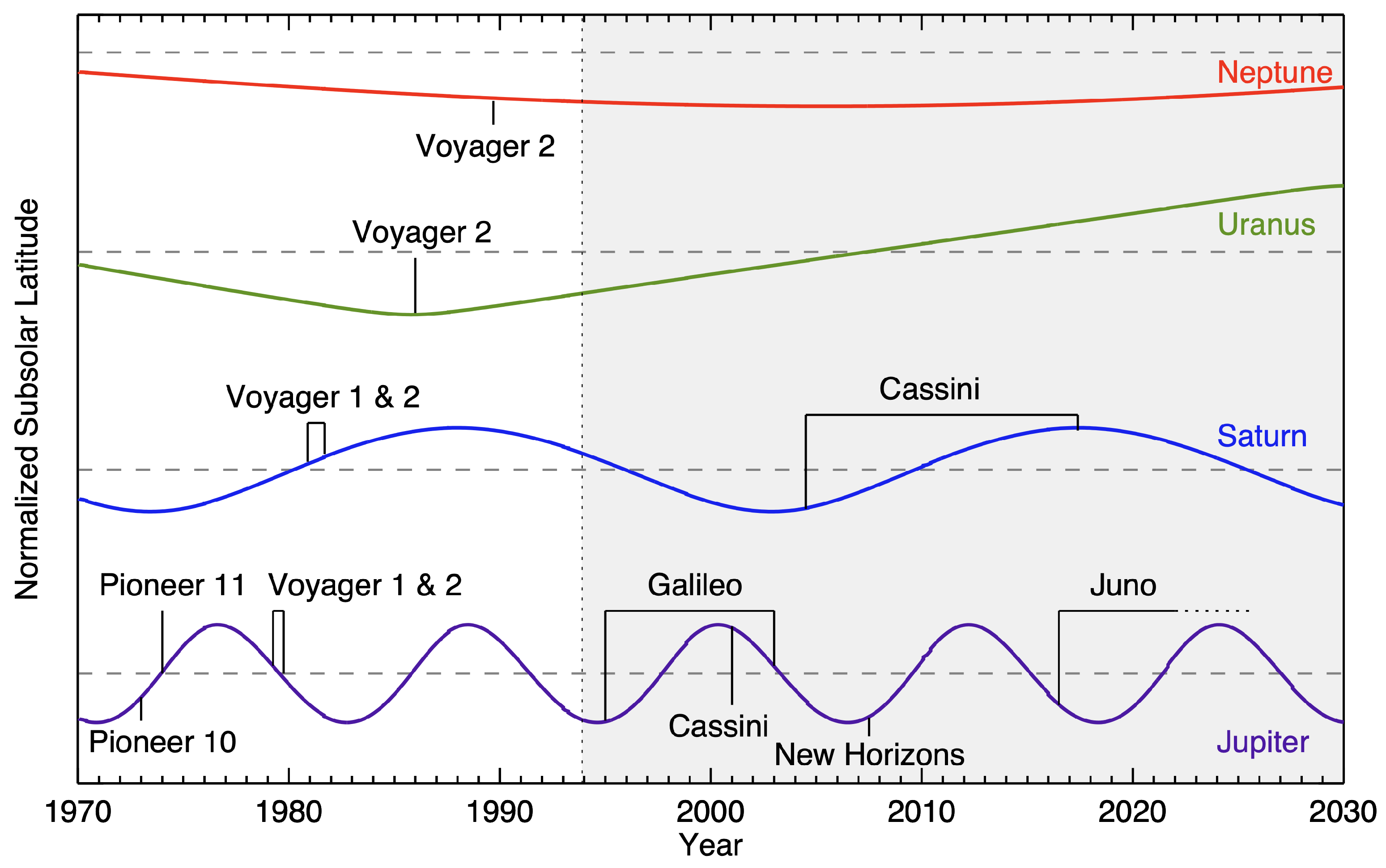
| Planet | Year | Mission |
|---|---|---|
| Jupiter | 1973 | Pioneer 10 Flyby |
| 1974 | Pioneer 11 Flyby | |
| 1979 | Voyager 1 Flyby | |
| 1979 | Voyager 2 Flyby | |
| 1993–1995 | Hubble Shoemaker-Levy 9 Campaign | |
| 1995–2003 | Galileo Mission | |
| 2000–2001 | Cassini Flyby | |
| 2007 | New Horizons Flyby | |
| 2015–present | Hubble OPAL Program | |
| 2016–present | Juno Mission | |
| Saturn | 1979 | Pioneer 11 Flyby |
| 1981 | Voyager 1 Flyby | |
| 1981 | Voyager 2 Flyby | |
| 2004–2017 | Cassini Mission | |
| 2018–present | Hubble OPAL Program | |
| Uranus | 1986 | Voyager 2 Flyby |
| 2006–2010 | Hubble Uranus Equinox Campaigns | |
| 2014–present | Hubble OPAL Program | |
| Neptune | 1989 | Voyager 2 Flyby |
| 2015–present | Hubble OPAL Program |
| Observatory (Aperture) | Angular Diffraction Limit (”) | Targets | AO System(s) | Imaging Instrument(s) |
|---|---|---|---|---|
| Keck (10 m) | 0.04 | Jupiter, Uranus, Neptune | Shack-Hartmann: NGS-AO, LGS-AO | NIRC2, NIRSPEC, KCAM [19,20,21,22,23,24,25,26,27,28,29,30,31,32,33,34,35,36,37,38,39,40,41] |
| Subaru (8.2 m) | 0.05 | Jupiter | Curvature sensor: AO188 | IRCS [42,43,44] |
| VLT (8.2 m) | 0.05 | Jupiter, Saturn, Uranus, Neptune | Shack-Hartmann and curvature sensors: MACAO, MAD, AOF/GALACSI | CAMCAO, CRIRES, SINFONI, MUSE [45,46,47,48,49,50,51] |
| Gemini-N (8.1 m) | 0.05 | Jupiter, Uranus, Neptune | Shack-Hartmann: ALTAIR | NIRI, NIFS [24,47,52,53,54,55] |
| Palomar (5.1 m) | 0.08 | Uranus, Neptune | Shack-Hartmann: PALM-241, PALM-3000 | P1640, PHARO [22,56] |
| CFHT (3.6 m) | 0.11 | Neptune | Curvature sensor: Hokupa’a | QUIRC [57,58] |
| Lick (3 m) | 0.13 | Neptune | Shack-Hartmann | ShARCS, LIRC2 [22,59] |
| Starfire (1.5) | 0.27 | Jupiter, Saturn | Shack-Hartmann | AOTF camera [60] |
Publisher’s Note: MDPI stays neutral with regard to jurisdictional claims in published maps and institutional affiliations. |
© 2022 by the authors. Licensee MDPI, Basel, Switzerland. This article is an open access article distributed under the terms and conditions of the Creative Commons Attribution (CC BY) license (https://creativecommons.org/licenses/by/4.0/).
Share and Cite
Simon, A.A.; Wong, M.H.; Sromovsky, L.A.; Fletcher, L.N.; Fry, P.M. Giant Planet Atmospheres: Dynamics and Variability from UV to Near-IR Hubble and Adaptive Optics Imaging. Remote Sens. 2022, 14, 1518. https://doi.org/10.3390/rs14061518
Simon AA, Wong MH, Sromovsky LA, Fletcher LN, Fry PM. Giant Planet Atmospheres: Dynamics and Variability from UV to Near-IR Hubble and Adaptive Optics Imaging. Remote Sensing. 2022; 14(6):1518. https://doi.org/10.3390/rs14061518
Chicago/Turabian StyleSimon, Amy A., Michael H. Wong, Lawrence A. Sromovsky, Leigh N. Fletcher, and Patrick M. Fry. 2022. "Giant Planet Atmospheres: Dynamics and Variability from UV to Near-IR Hubble and Adaptive Optics Imaging" Remote Sensing 14, no. 6: 1518. https://doi.org/10.3390/rs14061518
APA StyleSimon, A. A., Wong, M. H., Sromovsky, L. A., Fletcher, L. N., & Fry, P. M. (2022). Giant Planet Atmospheres: Dynamics and Variability from UV to Near-IR Hubble and Adaptive Optics Imaging. Remote Sensing, 14(6), 1518. https://doi.org/10.3390/rs14061518