Article

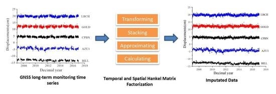
Missing Data Imputation in GNSS Monitoring Time Series Using Temporal and Spatial Hankel Matrix Factorization

1
College of Civil and Transportation Engineering, Shenzhen University, Shenzhen 518061, China
2
Institute of Urban Smart Transportation & Safety Maintenance, Shenzhen University, Shenzhen 518061, China
*
Author to whom correspondence should be addressed.
Remote Sens. 2022, 14(6), 1500; https://doi.org/10.3390/rs14061500
Submission received: 27 February 2022 / Revised: 16 March 2022 / Accepted: 17 March 2022 / Published: 20 March 2022
(This article belongs to the Special Issue Geodetic Observations for Earth System)

Abstract

:
GNSS time series for static reference stations record the deformation of monitored targets. However, missing data are very common in GNSS monitoring time series because of receiver crashes, power failures, etc. In this paper, we propose a Temporal and Spatial Hankel Matrix Factorization (TSHMF) method that can simultaneously consider the temporal correlation of a single time series and the spatial correlation among different stations. Moreover, the method is verified using real-world regional 10-year period monitoring GNSS coordinate time series. The Mean Absolute Error (MAE) and Root-Mean-Square Error (RMSE) are calculated to compare the performance of TSHMF with benchmark methods, which include the time-mean, station-mean, K-nearest neighbor, and singular value decomposition methods. The results show that the TSHMF method can reduce the MAE range from 32.03% to 12.98% and the RMSE range from 21.58% to 10.36%, proving the effectiveness of the proposed method.

Graphical Abstract

1. Introduction

With the development of remote sensing technologies, global navigation satellite system (GNSS) technology has been successfully applied in a variety of long-term monitoring areas. The U.S Global Positioning System (GPS) became the earliest, most well-established GNSS when it successfully launched 24 satellites in 1994. In addition, in recent decades, various countries have developed different GNSSs, such as Galileo in the European Union, GLONASS in Russia, and BeiDou Navigation Satellite System (BDS) in China. GNSSs are widely successfully applied in tectonic, glacial, seismic, civic infrastructural monitoring, etc. Furthermore, GNSS positioning in long-term monitoring is precise to within a few millimeters [1,2,3]. The Continuously Operating Reference Station (CORS) network is normally installed and archived in different organizations and countries for different application purposes. Pre-earthquake and coseismic ionosphere disturbances are analyzed using GNSS monitoring time series from the Crustal Movement Observation Network of China (CMONC), which was established in 2011 [4]. Moreover, long-term deformations are explored and analyzed depending on the regional GNSS CORS, such as the subsidence, faulting, and urban heat island studies from California, the Caribbean, and the Texas area [5,6,7,8]. However, a time series is influenced by many impact factors, which usually include linear and nonlinear variations. Thus, a post-processing method is required to analyze GNSS time series. Kaloop (2011) used GNSS monitoring solutions to estimate time-variable rates and to minimize the influence of traffic loads in bridge monitoring [9]. Seasonal uplift was introduced and analyzed by GNSS long-term monitoring time series in China and Nepal [10,11]. To explore precise deformation rates, several general packages have been written to post-process GNSS time series, such as tsfit/tsview from GAMIT/GLOBK [12], CATS [13], Hector [14], IDL package IGS [15], GITSTA [16], and TSAnalyzer [17]. These methods or tool packages focus on post-processing GNSS time series, such as deducting noise (white noise, colour noise, and random noise), removing common mode error, detecting outliers, calculating correlation coefficients, analyzing spectra, estimating distributions, and extracting periodic variations [18,19]. Obviously, these methods would show the best performance with continuous or no-gap GNSS time series data. If large data gaps appear, the overall performance of the post-processing of GNSS time series would be greatly degraded.
Unfortunately, missing data are very common in GNSS monitoring time series when collecting and processing raw data from GNSS stations. GNSS time series often present jumps due to physical or technical effects, such as tectonic jerks, sensor/hardware defects, and calibrations. As a result, they are strongly non-stationary. Therefore, filling the gaps in time series is not an easy task. The physical knowledge, spatiotemporal behavior, and auxiliary data are coherent with GNSS time series (such as VLBI measurements, InSAR time series, and Total Station), and other techniques (such as the Kalman filter and Least-Squares Spectral Analysis) could also decrease the influence of missing data. Ghaderpour (2021) proposed a method named jumps upon spectrum and trend in order to estimate the seasonal components of time series from original observational time series [20]. The method was established based on the Anti-Leakage Least-Squares Spectral Analysis (ALLSSA), which does not require any interpolation or gap filling [21]. However, data gap periods can vary from a few days to several months, and they could occupy from 5% to more than 30% of the whole dataset. The most common post-processing strategies choose to discard missing GNSS monitoring time series for convenient processing. Missing monitoring GNSS data could influence the precision of different deformation-monitoring applications. Filling missing data improves the extraction of the Common Mode Error (CME) and greatly reduces the Root Mean Square (RMS) of the residual velocity of incomplete position time series [22]. Ren et al. (2021) proposed the hybrid method of Multivariate Total Least-Squares (MTLS) and Improved Lomb–Scargle Periodogram (ILSP) to precisely analyze a scheme for a GNSS coordinate time series, which also needs to consider post-processing with missing data [23]. Li et al. (2020) filled the missing data and extracted Common Mode Errors from 44 continuous GNSS stations installed in southern California [24]. Velocity uncertainty represents an average reduction greater than 50% in north–south, east–west, and vertical components. Thus, it is necessary to develop an advanced method for missing data imputation in GNSS datasets.
Different imputation methods have been widely proposed for missing data recovery in recent years. The approaches to GNSS time series in previous studies can be generally summarized in the four types of methods discussed below. We categorize the existing literature into three research directions and briefly review them. The methods generally comprise time correlation, station correlation, K-nearest neighbor, and matrix factorization. Time-series correlations mainly use the methods of linear interpolation, cubic spline interpolation, polynomial interpolation, and sectioned Hermite interpolation [16]. Krypiak-Gregorczyk et al. (2017) applied thin-plate spline interpolation with multi-GNSS carrier-phase data to establish regional ionosphere modeling [25]. Moreover, cubic spline interpolation has been effectively used with global ionospheric map data to make comparisons with recorded GNSS ionospheric total electron content values [26]. These traditional methods are widely used to analyze various models with missing data interpolation. However, the methods mainly focus on a short period of missing data, and their lower effectiveness (such as accuracy and stabilization) is demonstrated when facing continuous GNSS coordinate missing data.
The second type considers spatial correlation from various monitoring stations. Balogun et al. (2021) considered spatial correlation with the cuckoo optimization algorithm to enhance the prediction of landslide susceptibility, and they achieved the best RMSE of 0.21 [27]. Liu et al. (2018) combined the Kriged Kalman Filter (KKF) and spatial influence analysis of the Southern California Integrated GPS Network (SCIGN) [28]. Benoist et al. (2020) simulated standard spatial filtering and established spatiotemporal covariance models of GNSS displacements [29]. This improved velocity determination, as proven by the datasets of 21 permanent GNSS stations. It could be found that the missing data in GNSS coordinate time series contain heterogeneous correlations. However, the various missing ratio patterns create a challenge for the method.
The third type considers the K-nearest neighbor. This method has the characteristics of simple implementation and outstanding performance. It has been successfully applied in low-dimensional and high-dimensional datasets, binary datasets, and multi-class datasets [30]. The optimal K values are selected for each missing datum result from the correlation between the missing datum and the datasets, reconstructing a sparse coefficient matrix between manually made missing data, original data, and all historical training data. The purpose of KNN is to explore the uncertainty of the various patterns or data induced by the different missing values and to effectively minimize missing data imputation errors [31,32,33]. The correlation between two instances needs to be measured using the distance function, and KNN is crucial to define the distance function.
Notably, with the development of computer science and computing power in recent decades, matrix decomposition methods have been widely applied in signal processing [34,35]. Principal component analysis (PCA) is more advanced in interpolating missing data in GNSS time series. Principal component analysis (PCA) was proposed to reduce the dimensionality of GNSS time series and to explore uncorrelated variables that successively maximize variance [36]. Dong et al. (2006) and Shen et al. (2014) extended PCA and IPCA to analyze GNSS monitoring time series with missing data to explore regional GNSS network displacements [5,22]. The conventional PCA algorithm was iterative until convergence with the missing data. The IPCA algorithm analyzes incomplete positional coordinate monitoring time series with the weighted quadratic norm of the principal component. In addition, PCA combined with Bayesian inference, called variational Bayesian principal component analysis (VBPCA), has been proposed to evaluate and interpolate missing data [24,37]. Missing data still influence the integrity level assessment of the GNSS monitoring model.
In view of this, Hankel Matrix Factorization could improve the effectiveness of completely missing data imputation [38]. Zhang et al. (2020) reduced the negative influence of missing samples when applying the instantaneous auto-correlation function reconstruction problem to rank minimization with a block Hankel matrix [39]. To achieve the sparsity-driven k-space interpolation method, the low-rank Hankel structure data matrix is constructed based on the annihilation property. This obtains a high-quality image, enrolling globally missing patterns, from a low-pixel raw image [40]. In addition, the method has also been developed and applied in geoscience applications. Chen et al. (2016) decomposed the block Hankel matrix to propose the damped rank-reduction method [41]. This method effectively reconstructs 5D seismic data with various percentages of missing traces. Considering mapping mantle seismic structure, singular value decomposition (SVD) is used to reconstruct missing observations by reducing the rank of the Hankel matrix [42]. In GNSS coordinate time series, the low-rank characteristics of the Hankel matrix are used to extract the GNSS seasonal signal with consideration of the missing data [43]. This shows that Hankel Matrix Factorization has a wide range of applications and obvious advantages in missing data interpolation. Thus, we develop a method based on Hankel Matrix Factorization and extend the correlation from a single temporal dimension to temporal and spatial dimensions for missing data imputation.
This paper is organized as follows: In Section 2, the collected real-world GNSS data, criteria, and processing steps are introduced, and the TSHMF method is presented. In Section 3, the proposed method is compared, and the results are presented. In the following section, the results of the model are discussed. The conclusion of the paper is drawn in the last section.

2. Materials and Methods

2.1. Problem Definiton
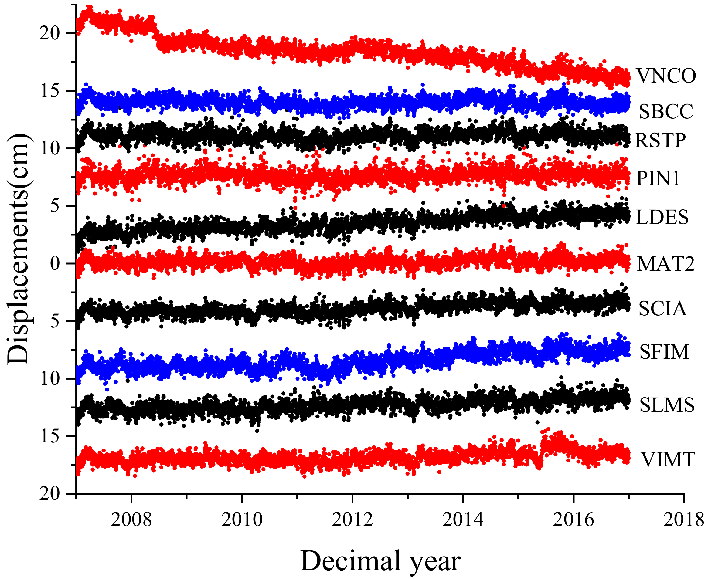
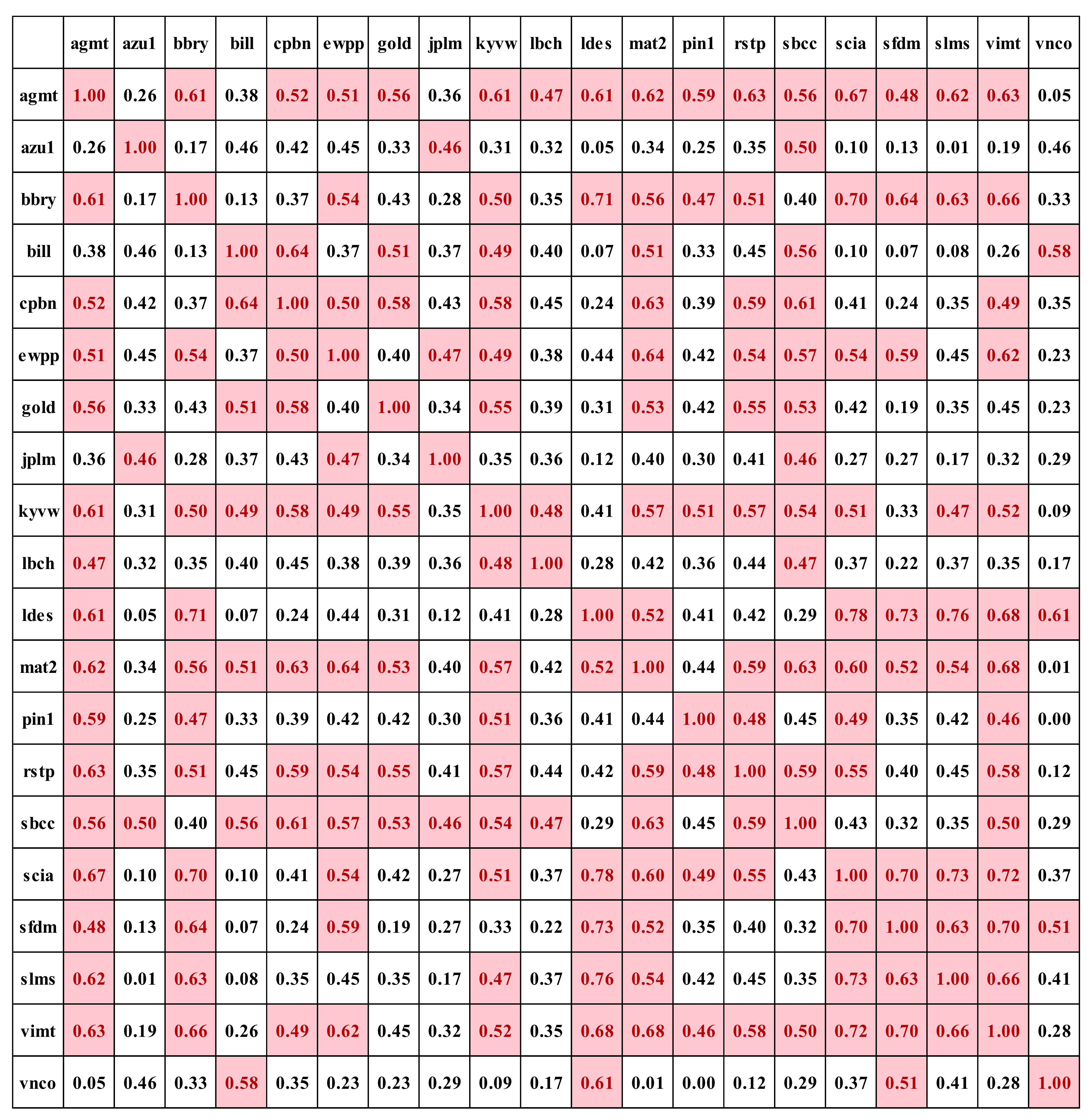
The definition of the general problem in missing data imputation for GNSS regional datasets is defined as follows: given the GNSS time series of length T , X = x 1 , x 2 , , x T , where x t R N is an N -dimensional column vector containing measurements of N stations at time t ; an indicating matrix I = 0 , 1 N × T , with i n , t = 0 if the n th dimension of x t is missing, and i n , t = 1 if the data are measured. The objective of GNSS data imputation is to estimate the missing values in X indicated by I .
According to the existing missing positions in GNSS datasets, the missing data can be categorized into four patterns, namely, the random missing pattern, time-continuous missing pattern, space-continuous missing pattern, and block missing pattern. We say i n , t , i n , t + 1 , , i n , t + l 1 is the time-continuous missing pattern of length l if i n , t , i n , t + 1 , , i n , t + l 1 = 0 ; i n , t , i n + 1 , t , , i n + l 1 , t is the space-continuous missing pattern of length l if i n , t , i n + 1 , t , , i n + l 1 , t = 0 . If the measurements present simultaneously time-continuous missing and space-continuous missing patterns, the pattern is called a block missing pattern. In a real-world GNSS dataset, these four patterns of missing data seldom appear alone.

2.2. Datasets

For the modeling, we need test data, which were collected and post-processed from the long-term monitoring task. Moreover, it was required that the data retain the shortcomings in the monitoring time series, such as unpredictable missing data and all original noise. Thus, we selected the GNSS long-term observations database, which has been archived in the Scripps Orbit and Permanent Array Center (SOPAC) since mid-1999. The data used for geodetic and seismic deformation monitoring consider constant offset, trend, annual, and semiannual terms [44] (Nikolaidis 2002). A total of 20 GNSS stations with a 10-year span (January 2007–December 2016) in the Southern California Integrated GNSS Network (SCIGN) were selected to test the model. The locations of the 20 GNSS stations in SCIGN are plotted in Figure 1. The selected GNSS data comprise 10 years of continuous data, and the average rate of missing data is less than 2%. To minimize the influence from the install design, the selected GNSS monitoring stations monument were Wyatt/Agnew drilled braced and installed on bedrock or low-rise buildings. The mounting type can greatly satisfy the stability of GNSS data influenced by unstable infrastructure. Based on the low missing rate and 10-year monitoring records, the GNSS dataset offers a stable data experimental environment to test the efficiency of the model. The raw data with clean tread north–south, east–west, and three vertical daily coordinate time series are free to download [45]. Significantly, the coordinate time series need to be processed using the mandatory and preliminary method. The daily North, East, Up (NEU) coordinates were post-processed using GAMIT/GLOBK from the raw observation file to the time series. Figure 2 shows the long-term monitoring vertical time series with the 20 selected GNSS stations.

2.3. Methods

Given the above problem definition, the proposed imputation method is presented in this subsection. The traditional matrix factorization-based approach is shown, and then the extension method for GNSS missing data is developed.

2.3.1. Matrix Factorization-Based Approach

In previous studies, matrix factorization-based approaches have been widely implemented to estimate and recover missing data in GNSS time series and have proved to be effective. In general, the matrix factorization-based approach models an N -dimensional GNSS measurement G R N × T as the product of low-rank matrix U R N × m and low-rank matrix V R m × T with m N and G U V . To solve the above U and V , the following objective function needs to be minimized:
arg   min U , V n , t H ( G n , t U n , : V : , t ) 2 + λ V T V V + λ U C U U + λ V C V V
where H is the set of measurement indexes, and G n , t is the element of G collected at time t by the GNSS station n ; u n , : and v : , t are the n th row and t th column of matrices U and V , respectively; T V V = t = 1 T 1 v : , t + 1 v : , t 2 is the regularization term for embedding the temporal correlation into the missing data imputation; C U U = U F 2 and C V V = V F 2 are two regularization terms used to avoid overfitting, where · F 2 represents the squared Frobenius norm; and λ V and λ U are two coefficients used to control the influence of the corresponding regularization term.
Although Equation (1) can solve most missing data imputation tasks, it does not consider spatial correlations, which are also critical for the analysis of real-world GNSS time series. As shown in Figure 3, the spatial correlations of several GNSS stations were calculated. It can be seen that most of the values are higher than 0.2, and more than half of the values are higher than 0.5. Moreover, the matrix factorization-based approach is not good at dealing with continuous missing data imputation. When the missing data present a time-continuous missing pattern, g n , t is continuously missing for most n 1 ,   N , so it is difficult to solve v : , t by minimizing g n , t u n , : v : , t 2 . The challenge for the space-continuous missing pattern is the same as that for the time-continuous missing pattern. Motivated by the above two challenges of the traditional matrix factorization-based approach, we proposed Temporal and Spatial Hankel Matrix Factorization (TSHMF) for GNSS continuous missing data imputation, simultaneously considering temporal and spatial correlations.

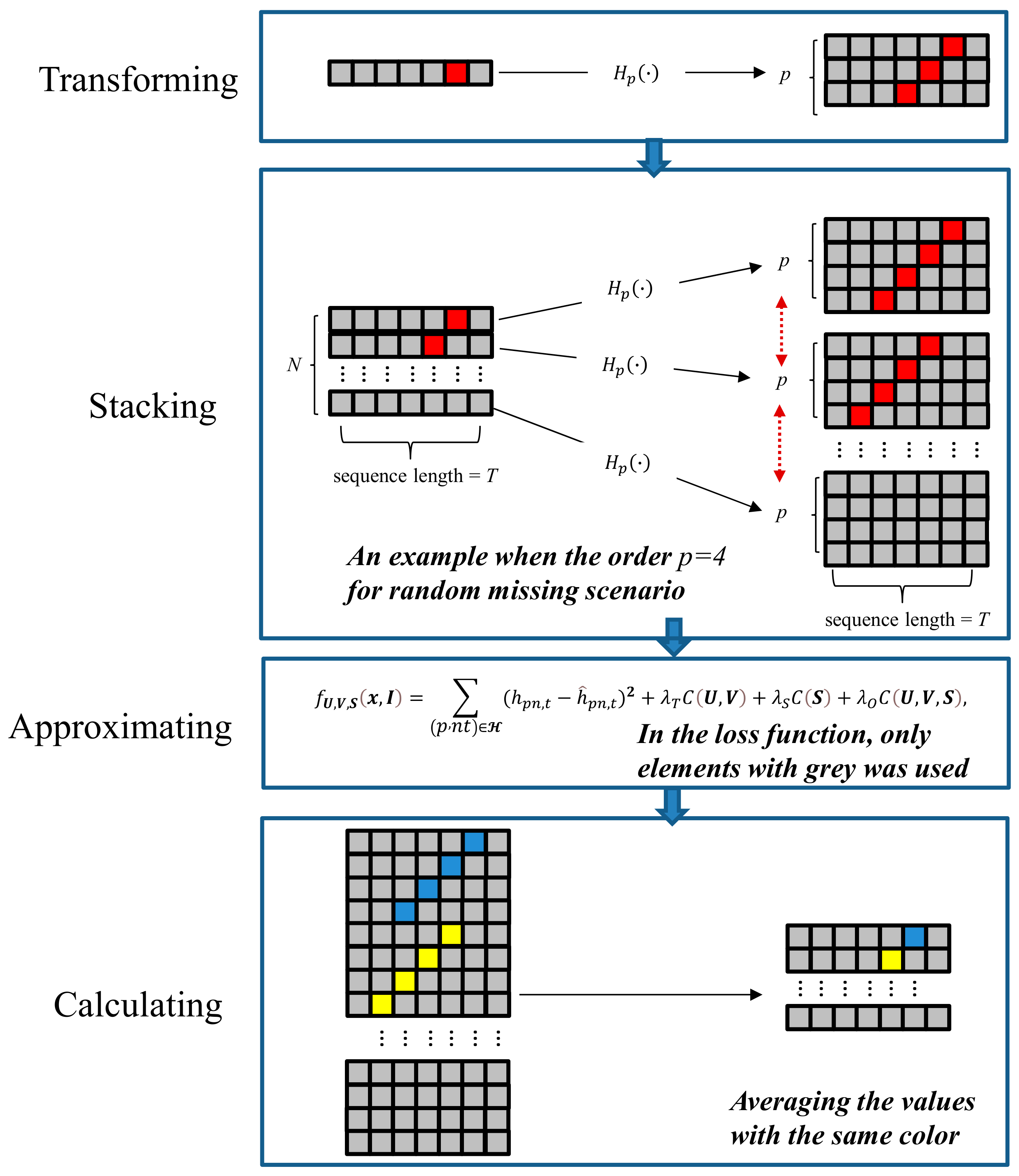
2.3.2. Temporal and Spatial Hankel Matrix Factorization

The procedures of the proposed TSHMF are shown in Figure 2, and they involve four steps: transforming, stacking, approximating, and calculating. In the first step, the GNSS time series of station n with missing data should be transformed into Hankel matrix H p n , where p is the order. In the second step, to consider the spatial correlations of regional GNSS time series during the imputation process, the Hankel matrices of N stations are stacked as the matrix H P R P × T , and P = p × n . In the third step, H P is approximated with matrix H ^ so that H ^ = U V + S , where U R P × m and V R m × T are two low-rank matrices indicating the latent and temporal correlations, respectively. The matrix S is added to consider the spatial correlations among regional GNSS time series. In the fourth step, the missing values in the original matrix G are calculated.
As shown in Figure 4, to approximate the matrix with missing values, U , V , and S should be solved, and the following objective function is used:
f U ,   V , S x , I = p n , t H ( h p n , t h ^ p n , t ) 2 + λ T C U , V + λ S C S + λ O C U , V , S
where H is the set of indexes corresponding to the measured values in H P ; h p n , t and h ^ p n , t   are the p n , t th elements in H P and H , respectively. C U , V , C S , and C U , V , S are three constraints for temporal correlation, spatial correlation, and avoiding overfitting, respectively, with λ T , λ S , and λ O being the coefficients. More specifically, the main term and the three constraints in the objective function are described as follows:
(1)
Main term: The main term in the objective function is used to estimate the error of the imputation during the optimization process; that is, p n , t H ( h p n , t h ^ p n , t ) 2 measures the error of approximating H P with H ^ , where h ^ p n , t = u p n , : v : , t + s p n , t .
(2)
Temporal correlation: The second term λ T C U , V is used to capture the temporal correlations among the GNSS time series, defined as
C U , V = p n = 1 P t = 2 T u p n , : v : , t u p n , : v : , t 1 2
This term can restrict the solution of U , V to remain as the temporal correlations of the raw data.
(3)
Spatial correlation: The third term is implemented to capture the spatial correlations among the regional GNSS time series, defined as
C S = p n = 1 P u p n , : 1 N n = 1 N u p n + n 1 × p , : 2
(4)
Avoiding overfitting: The final term is implemented to control the balance of the spatial and temporal correlations by avoiding U V = 0 and S = 0 , defined as
C U , V , S = U F 2 + V F 2 + S F 2  

2.3.3. Solution of Factorization

To solve U , V , and S , the above objective function should be minimized. Because the function is nonconvex, the stochastic gradient decent (SGD) approach is applied according to the following rules:
u p n , : u p d a t e = u p n , : + η [ e p n . t v : , t T λ O u p n , : λ T u p n , : v : , t u p n , : v : , t 1 v : , t v : , t 1 T
v : , t u p d a t e = v : , t + η [ e p n . t u p n , : T λ O v : , t λ T 2 u p n , : v : , t u p n , : v : , t 1 u p n , : v : , t + 1 u p n , : T ]  
s p n , : u p d a t e = s p n , : + η e p n . : λ O s p n , : λ S u p n , : 1 N n = 1 N u p n + n 1 × p , :  
where e p n . : = h p n , : h ^ p n , : ; η is a small positive value to control the step size of each round for updating. Based on previous studies, η is set as 0.01 in this paper. To speed up the optimization of the algorithm, U and V are initialized using the PCA method, and S is initialized with random values. After this step, the proposed method is iteratively updated according to Algorithm 1 until coverage. The stop condition is empirically set as the difference between two consecutive iterations of less than 0.01 in the experiment.
Algorithm 1 Missing data imputation for regional GNSS time series using TSHMF
Input: Regional GNSS time series with missing values X = x 1 , x 2 , , x T the station index of the times series, the indicator matrix, I , λ T ,   λ S ,   λ O ,   η ,   η and the stop condition.
Output: The missing values in the Hankel matrix
1: Obtain the longest duration of time-continuous missing l c o n and set p l c o n + 1
2: Obtain the Hankel matrix H p as demonstrated in the paper and Figure 2
3: Initial U , V , and S
4: repeat
5: for all p n , t H do
6:  Update u p n , : following the equation
7:  Update v : , t following the equation
8:   Update s p n , : following the equation
9: end for
10: until stop condition is reached
11: return the imputation of all missing values
After the imputation of the Hankel matrix, the missing values in the raw matrix X are calculated by averaging the values of the corresponding element in H p .

3. Results and Discussion

To test the precision and effectiveness of the method in long-term monitoring GNSS time series with missing data, this section compares the ability of different methods to impute the data in two common scenarios. The four types of general missing imputation methods (TM, SM, KNN, and SVD) are used as benchmark models to evaluate the TSHMF method. Moreover, this section evaluates the impact of temporal and spatial correlations.

3.1. Experimental Design and Evaluation Criteria

3.1.1. Generation of Missing Values

Missing data occur randomly, and they are unpredictable. Thus, the missing data properties in this paper need to be established first. In this paper, we simulate various missing statuses in real data and verify real-world datasets. Two different types of missing data scenarios, namely, random missing and continuous missing scenarios, are observed, and they can be described as follows:
(1)
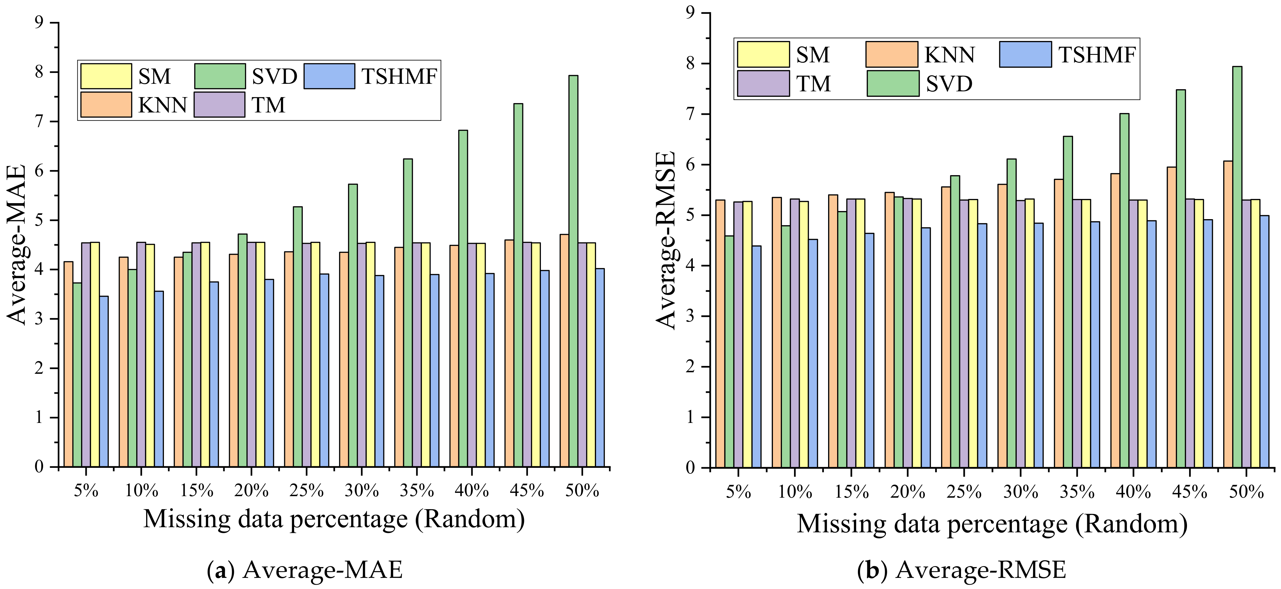
Totally random missing scenario: This means that the missing observations are independent and randomly missing. This scenario usually shows isolated missing observations, resulting from the solutions removed, sudden satellite signal interruption, etc. In the random missing scenario, we manually extracted the random missing data in each stations. The random missing ratios in this model were manually removed from 5 to 50%, with an increasing interval of 5% in each matrix.
(2)
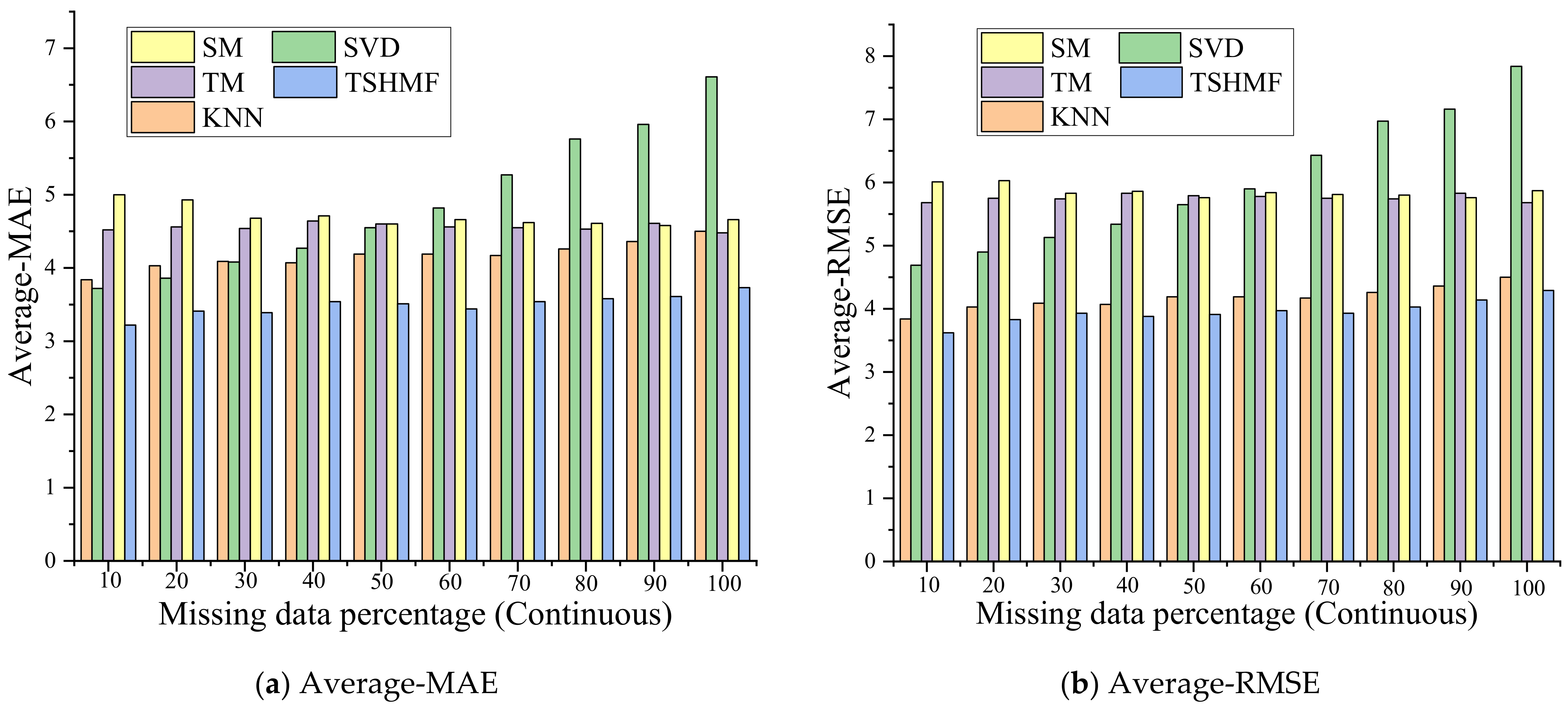
Continuous missing scenario: This means that the missing data are detected with a small group of sequential points lost at one station, resulting from a power cut, device replacements, etc. In this scenario, we divided all ten-year periods of data into a single year, and the missing part was randomly scattered in each station within each year. The number of consecutive missing points ranges from 10 to 100, with 10 as the interval.

3.1.2. Evaluation Criteria

Two evaluation criteria, namely, Root-Mean-Square Error (RMSE) and Mean Absolute Error (MAE), were used to evaluate the performance of the introduced imputation method and compare its performance to that of the conventional imputation method. The equations of the two criteria are as follows:
R M S E = 1 N i = 1 N r i m i 2  
M A E = 1 N i = 1 N r i m i   10
where N is the total number of missing values, r i is the i th imputed value, and m i is the i th measured value.

3.1.3. Benchmark Models

The missing value imputation model has been widely developed in recent years. The most common four types of missing data imputation models comprise time correlation, station correlation, K-nearest neighbor, and matrix factorization. Specifically, we selected the time-mean (TM), station-mean (SM), K-nearest neighbor (KNN), and singular value decomposition (SVD) methods to be the benchmark models in order to evaluate the performance of the proposed model. The TM and SM methods are traditional and widely used to impute missing values. SVD is also one of the most common methods in matrix factorization. Thus, we enrolled these four methods in the benchmark models. The details are as follows:
The time-mean (TM) method simply estimates the missing values using the mean of the observed values of the time series in the same station.
The station-mean (SM) method simply estimates the missing values using the mean of the observed values in other stations at the same timestamp.
The K-nearest neighbor (KNN) method is simple and intuitive, and it utilizes the mean of the K-nearest values to impute the missing value. It has been found that the accuracy of the imputation cannot significantly improve when K is more than 7, so K was set as 7.
The singular value decomposition (SVD) method is one of the most important matrix decomposition methods in linear algebra. In this experiment, we selected the first singular value and set the others as 0.

3.2. Random Missing Data Scenario

To adequately verify the proposed applicability of the method in different long-term GNSS time series, we used the averages MAE and RSME of all 20 GNSS stations as indexes. These indicators can interpret the accuracy of the different methods within all 20 selected GNSS stations. Figure 5 shows the average MAE and RMSE values calculated from all selected GNSS time series processed by the KNN, SVD, TM, SM, and proposed TSHMF methods. The results show that the SVD method exhibits poorer performance as the missing ratio increases. It can be seen that the errors rapidly grow, indicating that the method is only fit for a random missing ratio under 15%. Moreover, the KNN, TM, and SM methods show the same level of performance trends in RSME and MAE. Notably, the proposed TSHMF method has the best performance in all missing ratio settings. The TSHMF has a reduced MAE and RMSE of 20% and 15%, respectively, compared to the benchmark methods in the random missing data scenario.
The missing data imputation is critical for moving monitoring time series and influences our understanding of tectonic movement in the target area. The experimental region has been impacted by the collision of the North American plate with the Pacific/Farallon active ridge in the Neogene [46]. Theoretically, when the target deformation is more rigid, long-term monitoring time series are more stable, and the missing data imputation would become more feasible. Thus, we selected the VNCO station due to the fact that it has the fastest subsidence rate compared with all 20 selected GNSS stations. It has a subsidence rate with respect to North American datum of −4.24 ± 0.46 mm/year in the southern California region (Figure 3). It shows long-term inner deformation movements in the local southern California region. It is clear that the VNCO station has the highest average MAE and RMSE in all missing ratios compared with other GNSS monitoring stations. In the modeling, for the VNCO station, the averages of the MAE using the KNN, SVD, TM, SM, and TSHMF methods are 6.61, 17.62, 10.84, 10.91, and 6.41, respectively. Moreover, for the VNCO station, the averages of the RMSE using the KNN, SVD, TM, SM, and TSHMF methods are 8.81, 19.14, 14.09, 14.19, and 8.70, respectively. Obviously, the proposed TSHMF method shows the best performance when compared with the other benchmark models.
The introduced imputation method (TSHMF) is compared with the traditional method according to the results of the 20 GNSS stations with a 10-year monitoring time series. To further verify the stabilization applied in the random missing scenarios, all methods were quantitatively analyzed. In this section, we set the standard deviation (STD) to evaluate the stabilization of the different methods with various missing ratios. The STD is calculated from the MAE and RMSE values from each of the 20 selected permanent GNSS stations. As shown in Table 1, the KNN and TSHMF methods have the same level of quantitative value in STD and have distinct values, and both methods have smaller values than those of SVD, TM, and SM. The STD values of KNN are small, and they are smaller in the 20%, 30%, 35%, 40%, 45%, and 50% missing ratios in MAE and in the 15%, 20%, 30%, 35%, 40%, 45%, and 50% missing ratios in RMSE. However, the difference in STD values between the KNN and TSHMF methods is smaller than 0.1. This shows that the KNN and TSHMF methods have the same steady performance in random missing scenarios. Moreover, the STD values of the SVD method grow as the missing ratio increases. In summary, considering all statistical analyses with the indicators of MAE, RMSE, and STD, the proposed TSHMF model demonstrates the highest stabilization and performance when compared with all methods in the random missing scenarios.

3.3. Continuous Missing Data Scenario

In this section, the same criteria as those of the random missing scenarios are used to quantitatively evaluate the performance of the KNN, SVD, TM, SM, and TSHMF methods. Figure 6 shows the average MAE and RMSE of each of the 20 permanent GNSS stations to evaluate accuracy performance. Based on the results shown in Figure 6, the KNN, TM, and SM methods show various accuracies in different ratios of continuous missing scenarios. For example, the MAE average of KNN is 3.84, and the MAE average of SM is 5.0. The KNN has obvious advantages in the 5% continuous missing scenario. In the 50% ratio continuous missing scenario, the KNN and SM methods have almost the same performance. Furthermore, the SVD method exhibits poorer performance as the continuous missing ratio increases. However, this method has acceptable performance when it is applied under missing ratios lower than 25%. Notably, compared with the KNN, TM, and SM methods, the TSHMF method shows the best performance in all continuous missing ratio scenarios. When compared with the benchmark methods, it reduces the MAE and RMSE by approximately 24% and 28%, respectively.
In the continuous missing data scenario, the VNCO has to also be tested similarly to how it was tested in the random missing scenario due to the faster subsidence rate in the 20 selected GNSS stations with respect to the North American datum. Generally, it is different in the random missing scenario, because some of the reasons for a continuous missing pattern result from device replacements or disasters, such as landslides and earthquakes [47]. The status normally lasts a shorter or longer period of time. Thus, it is also critical for a moving station, such as the VNCO station, even referred to the local region (Figure 3). In the continuous scenario, for the VNCO station, the averages of MAE using the KNN, SVD, TM, SM, and TSHMF methods are 6.16, 13.35, 10.83, 11.08, and 5.53, respectively. Moreover, for the VNCO station, the averages of RMSE using the KNN, SVD, TM, SM, and TSHMF methods are 7.30, 24.24, 13.34, 14.51, and 6.83, respectively. The results prove that the proposed TSHMF model has the best performance in all various continuous missing ratios in GNSS long-term monitoring coordinate time series.
For the method of stabilization in the continuous missing scenario, the same quantitative analysis criteria that were applied in the random missing scenarios are also applied in the continuous missing scenarios. Table 2 shows the STD values of the MAE and RMSE from each of the 20 selected permanent GNSS stations in various continuous missing ratios. The STD values show that the KNN method only has two patterns and three patterns in the continuous missing ratios, which is somewhat better than the proposed TSHMF method in MAE and RMSE, respectively. Generally, considering the STD values from all ten various continuous missing ratios, the TSHMF method shows the best performance in the STD values of MAE and RMSE when compared to all methods. Notably, the STD values of the SVD method still grow as the continuous missing ratio increases. However, the proposed TSHMF method maintains stable STD values in both MAE and RMSE. This also indicates that the TSHMF method has the highest stabilization compared with the other benchmark methods in continuous missing scenarios.

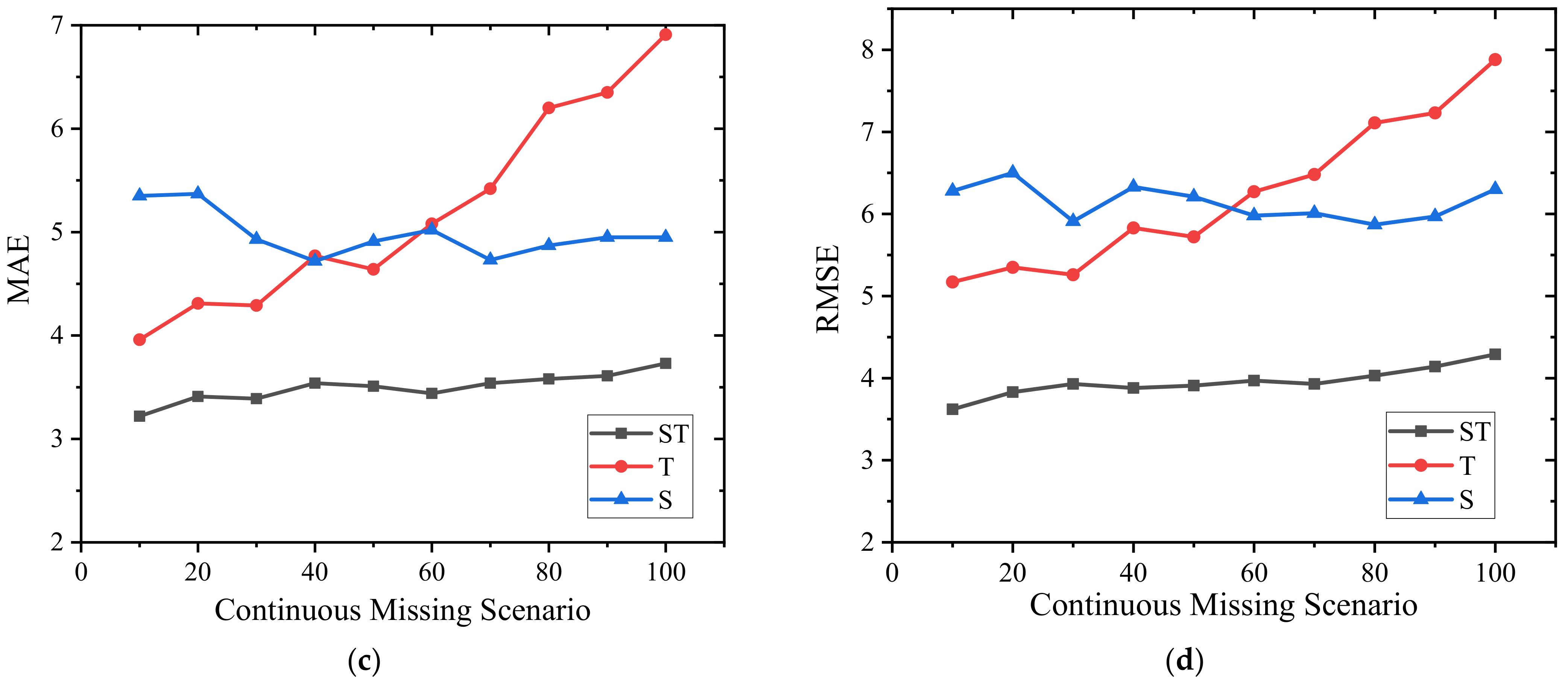
3.4. The Impact of Temporal and Spatial Correlations

Long-term monitoring time series have the characteristics of temporal and spatial correlations, especially in rigid microplates. The purpose of long-term geoscience monitoring time series is to record the displacements of the target area (shallow and deep) as time goes on. This presents the property of temporal correlation. Moreover, monitoring stations are normally installed in the local area and have the same moving rate as in the micro-tectonic area. Theoretically, a monitoring station in the same area could have the same moving rate as spatial correlation in the local region. However, real-world monitoring shows that the deformation value is different. Thus, we have to consider both temporal and spatial factors.
In Figure 7, both the spatial and temporal correlations are considered in the various missing data imputations. ST represents the spatial and temporal correlations, which are both considered in the modeling. T represents consideration of only the temporal correlation, and S represents consideration of only the spatial correlation. As the results show, ST showed the best performance in all random and continuous missing scenarios. The averages of MAE and RMSE with ST improved by 20.31% and 17.22%, and 20.76% and 17.49% compared with temporal or spatial correlation in random missing scenarios, respectively. In the continuous missing scenarios, the averages of MAE and RMSE improved by 32.67% and 36.52%, and 29.78% and 35.54% compared with T and S, respectively. Interestingly, the spatial correlation and temporal correlation have similar MAE and RMSE values in the random missing values. This shows that the influence weight with consideration of only the spatial or temporal correlation is similar in the random missing scenario. However, the MAE and RMSE values that only consider the temporal correlation grow greatly when a continuous missing value beyond 60 is recorded in one decimal year. This shows that only considering the temporal correlation results in bad performance when the monitoring time series have continuous missing records longer than 60 days. Thus, under various missing scenario conditions, it is hard to prove whether the consideration of only temporal correlation or spatial correlation has greater weight in long-term monitoring time series. A full analysis of long-term monitoring time series needs to consider both temporal and spatial correlations.
In the results, it can be found that simultaneously considering the temporal and spatial correlations can improve the accuracy of the imputation. The reason for this is that GNSS long-term monitoring time series are strongly non-stationary because of annual/semi-annual and other high-frequency components due to atmospheric effects, tides (when the stations are near coastal areas), etc. Only using the available time series data to fill in the missing values is not recommended unless the time series components are known to be stable/stationary. The findings of this research are in line with those of some previous studies [21]. Using techniques such as cross-wavelet analysis with the aid of spatiotemporal behavior could be extremely helpful for the estimation of missing values.

4. Conclusions

Long-term GNSS observation data provide an efficient tool for geodesy, tectonic, and structural health monitoring. Missing data still influence the analysis of GNSS time series. In this study, we proposed the method of Temporal and Spatial Hankel Matrix Factorization for GNSS long-term monitoring coordinate time series. The method, trained with the Hankel matrix, is iteratively updated and considers the temporal and spatial correlations in GNSS time series. In this study, we conducted an experiment with random missing patterns and continuous missing patterns from 20 permanent GNSS stations with 10-year periods. The GNSS stations are installed in various infrastructures with different monitoring targets. The results show that the TSHMF method could improve the missing data imputation compared with the time-mean (TM) method, station-mean (SM) method, K-nearest neighbor (KNN) method, and singular value decomposition (SVD) method. The average Mean Absolute Error (MAE) and Root-Mean-Square Error (RMSE) were reduced by 20% when using the TSHMF method. Based on the results, the following conclusions can be drawn:
(1)
In real-world long-term tectonic monitoring missing data imputation, the method shows the best applicability in stable local regions. The TSHMF method considers both the long-term stable and moving monitoring time series with respect to the regional area. The result shows the highest accuracy in long-term deformation monitoring when compared with the benchmark models (TM, SM, KNN, and SVD). The proposed method could be used in various geodetic long-term monitoring applications.
(2)
The results show the robust performance of the proposed method, which enrolled various ratios of missing data in the random missing scenario and continuous missing scenario. Both temporal correlation and spatial correlation can contribute to the accuracy of missing value imputation, further proving that the simultaneous consideration of temporal and spatial correlations is necessary in regional GNSS time series modeling.
(3)
The present paper proves the limitation of only considering a single monitoring station in geoscience long-term time series analysis. To achieve a high-accuracy analysis, not only did the raw data from the station need to be post-processed, but also, the results from a nearby station, which was installed in a rigid area, were also needed for the post-processing method. Regional analysis would further improve the accuracy of single long-term monitoring time series results.
Future studies could consider the application of the proposed model in a larger regional area or various tectonic plates. In addition, GNSS displacement time-series measurements usually contain error bars. Obviously, the measurement with high errors contributes less to the estimation of trends and seasonal components and vice versa. Full consideration of the influence of error bars could also improve the analysis of long-term monitoring time series. In order to further improve the quality of long-term monitoring time series, a future updated method could also consider these error bars and, more generally, the covariance matrices associated with the time series.

Author Contributions

L.L. and H.L.: conceptualization, methodology, data curation, and writing—original draft preparation. H.L.: visualization and investigation. L.L.: supervision. All authors have read and agreed to the published version of the manuscript.

Funding

The authors gratefully acknowledge support from the National Key R&D Program of China (No. 2019YFB2102700), the China Postdoctoral Science Foundation funded project (No. 2020M682883), Shenzhen Municipal Science and Technology Innovation Committee (No. 20200812102651001), and Guangdong Basic and Applied Basic Research Foundation (No. 2020A1515110438).

Data Availability Statement

Data are available in a publicly accessible repository (see Acknowledgments).

Acknowledgments

The authors acknowledge Guoquan Wang (the University of Houston) for providing the PPP solution data quality check for this study. The first author also thanks the UNAVCO and the Nevada Geodetic Laboratory (NGL) at the University of Nevada for sharing their GPS products with the public; Data is available through http://geodesy.unr.edu/ (accessed on 1 March 2022).

Conflicts of Interest

The authors declare no conflict of interest. We declare that we do not have any commercial or associative interest that represents a conflict of interest in connection with the work submitted.

Abbreviations

The following abbreviations are used in this manuscript:
ALLSSAAnti-Leakage Least-Squares Spectral Analysis
BDSBeiDou Navigation Satellite System
CMONCCrustal Movement Observation Network of China
CORSContinuously Operating Reference Station
CMECommon Mode Error
GNSSGlobal navigation satellite system
GPSGlobal Positioning System
ILSPImproved Lomb–Scargle Periodogram
InSARInterferometric Synthetic Aperture Radar
IPCAIncremental principal component analysis
KKFKriged Kalman Filter
KNNK-nearest neighbor
LSWALeast-squares wavelet analysis
MAEMean Absolute Error
MTLSMultivariate Total Least-Squares
PCAPrincipal component analysis
RMSRoot Mean Square
SSpatial correlation
SCIGNSouthern California Integrated GPS Network
SMStation mean
STSpatial and temporal correlations
SOPACScripps Orbit and Permanent Array Center
SVDSingular value decomposition
TTemporal correlation
TMTime mean
TSHMFTemporal and Spatial Hankel Matrix Factorization
VBPCAVariational Bayesian principal component analysis

References

  1. Pourghasemi, H.R.; Kariminejad, N.; Gayen, A.; Komac, M. Statistical functions used for spatial modelling due to assessment of landslide distribution and landscape-interaction factors in Iran. Geosci. Front. 2020, 11, 1257–1269. [Google Scholar] [CrossRef]
  2. Liu, H.; Yang, L.; Li, L. Analyzing the Impact of Climate Factors on GNSS-Derived Displacements by Combining the Extended Helmert Transformation and XGboost Machine Learning Algorithm. J. Sens. 2021, 3, 2256. [Google Scholar] [CrossRef]
  3. Li, L.; Lin, X.; Liu, H.; Lu, W.; Zhou, B.; Zhu, J. Displacement Data Imputation in Urban Internet of Things System Based on Tucker Decomposition with L2 Regularization. IEEE Internet Things J. 2022, 38, 2782. [Google Scholar] [CrossRef]
  4. Shi, K.; Liu, X.; Guo, J.; Liu, L.; You, X.; Wang, F. Pre-Earthquake and Co-seismic Ionosphere Disturbances of the Mw 6.6 Lushan Earthquake on 20 April 2013 Monitored by CMONOC. Atmospheres 2019, 10, 216. [Google Scholar] [CrossRef] [Green Version]
  5. Dong, D.; Fang, P.; Bock, Y.; Webb, F.; Prawirodirdjo, L.; Kedar, S.; Jamason, P. Spatiotemporal filtering using principal component analysis and Karhunen–Loeve expansion approaches for regional GPS network analysis. J. Geophys. Res. 2006, 111, 1581–1600. [Google Scholar] [CrossRef] [Green Version]
  6. Liu, H.; Wang, G. Relative motion between St. Croix and the Puerto Rico-Northern Virgin Islands block derived from continuous GPS observations (1995–2014). Int. J. Geophys. 2015, 37, 2671. [Google Scholar] [CrossRef] [Green Version]
  7. Wang, G.; Liu, H.; Mattioli, G.S.; Miller, M.M.; Feaux, K.; Braun, J. CARIB18: A stable geodetic reference frame for geological hazard monitoring in the Caribbean region. Remote Sens. 2019, 11, 680. [Google Scholar] [CrossRef] [Green Version]
  8. Mendez-Astudillo, J.; Lau, L.; Tang, Y.T.; Moore, T. A new Global Navigation Satellite System (GNSS) based method for urban heat island intensity monitoring. Int. J. Appl. Earth Obs. Geoinf. 2021, 94, 102222. [Google Scholar] [CrossRef]
  9. Kaloop, M.R.; Li, H. Sensitivity and analysis GPS signals based bridge damage using GPS observations and wavelet transform. Measures 2011, 44, 927–937. [Google Scholar] [CrossRef]
  10. Liu, B.; Dai, W.; Liu, N. Extracting seasonal deformations of the Nepal Himalaya region from vertical GPS position time series using independent component analysis. Adv. Space Res. 2017, 60, 2910–2917. [Google Scholar] [CrossRef]
  11. Yan, J.; Dong, D.; Bürgmann, R.; Materna, K.; Tan, W.; Peng, Y.; Chen, J. Separation of sources of seasonal uplift in China using independent component analysis of GNSS time series. J. Geophys. Res. Solid Earth 2019, 124, 11951–11971. [Google Scholar] [CrossRef]
  12. Herring, T.A.; King, R.W.; McClusky, S.C. Introduction to Gamit/Globk; Massachusetts Institute of Technology: Cambridge, MA, USA, 2010. [Google Scholar]
  13. Williams, S.D. CATS: GPS coordinate time series analysis software. GPS Solut. 2008, 12, 147–153. [Google Scholar] [CrossRef]
  14. Bos, M.S.; Fernandes, R.M.S.; Williams, S.D.P.; Bastos, L. Fast error analysis of continuous GNSS observations with missing data. J. Geod. 2013, 87, 351–360. [Google Scholar] [CrossRef] [Green Version]
  15. Tian, Y. iGPS: IDL tool package for GPS position time series analysis. GPS Solut. 2011, 15, 299–303. [Google Scholar] [CrossRef]
  16. Goudarzi, M.A.; Cocard, M.; Santerre, R.; Woldai, T. GPS interactive time series analysis software. GPS Solut. 2013, 17, 595–603. [Google Scholar] [CrossRef]
  17. Wu, D.; Yan, H.; Shen, Y. TSAnalyzer, a GNSS time series analysis software. GPS Solut. 2017, 21, 1389–1394. [Google Scholar] [CrossRef]
  18. Didova, O.; Gunter, B.; Riva, R.; Klees, R.; Roese-Koerner, L. An approach for estimating time-variable rates from geodetic time series. J. Geod. 2016, 90, 1207–1221. [Google Scholar] [CrossRef] [Green Version]
  19. He, X.; Yu, K.; Montillet, J.P.; Xiong, C.; Lu, T.; Zhou, S.; Ma, X.; Cui, H.; Ming, F. GNSS-TS-NRS: An Open-source MATLAB-Based GNSS time series noise reduction software. Remote Sens. 2020, 12, 3532. [Google Scholar] [CrossRef]
  20. Ghaderpour, E. Least-squares wavelet and cross-wavelet analyses of VLBI baseline length and temperature time series: Fortaleza–Hartebeesthoek–Westford–Wettzell. Publ. Astron. Soc. Pac. 2021, 133, 014502. [Google Scholar] [CrossRef]
  21. Ghaderpour, E. JUST: MATLAB and python software for change detection and time series analysis. GPS Solut. 2021, 25, 1–7. [Google Scholar] [CrossRef]
  22. Shen, Y.; Li, W.; Xu, G.; Li, B. Spatiotemporal filtering of regional GNSS network’s position time series with missing data using principle component analysis. J. Geod. 2014, 88, 1–12. [Google Scholar] [CrossRef]
  23. Ren, Y.; Wang, H.; Lian, L.; Wang, J.; Cheng, Y.; Zhang, Y.; Zhu, W.; Zhang, S. A method based on MTLS and ILSP for GNSS coordinate time series analysis with missing data. Adv. Space Res. 2021, 68, 3546–3561. [Google Scholar] [CrossRef]
  24. Li, W.; Jiang, W.; Li, Z.; Chen, H.; Chen, Q.; Wang, J.; Zhu, G. Extracting Common Mode Errors of Regional GNSS Position Time Series in the Presence of Missing Data by Variational Bayesian Principal Component Analysis. Sensors 2020, 20, 2298. [Google Scholar] [CrossRef] [PubMed] [Green Version]
  25. Krypiak-Gregorczyk, A.; Wielgosz, P.; Borkowski, A. Ionosphere model for European region based on multi-GNSS data and TPS interpolation. Remote Sens. 2017, 9, 1221. [Google Scholar] [CrossRef] [Green Version]
  26. Ansari, K.; Sharma, S.K. Ionospheric TEC variation based on GNSS data over the Arabian Peninsula and validation with the cubic spline interpolated GIM model. Adv. Space Res. 2021, 68, 3814–3820. [Google Scholar] [CrossRef]
  27. Balogun, A.L.; Rezaie, F.; Pham, Q.B.; Gigović, L.; Drobnjak, S.; Aina, Y.A.; Panahi, M.; Yekeen, T.S.; Lee, S. Spatial prediction of landslide susceptibility in western Serbia using hybrid support vector regression (SVR) with GWO, BAT and COA algorithms. Geosci. Front. 2021, 12, 101104. [Google Scholar] [CrossRef]
  28. Liu, N.; Dai, W.; Santerre, R.; Kuang, C. A MATLAB-based Kriged Kalman Filter software for interpolating missing data in GNSS coordinate time series. GPS Solut. 2018, 22, 1–8. [Google Scholar] [CrossRef]
  29. Benoist, C.; Collilieux, X.; Rebischung, P.; Altamimi, Z.; Jamet, O.; Métivier, L.; Chanard, K.; Bel, L. Accounting for spatiotemporal correlations of GNSS coordinate time series to estimate station velocities. J. Geodyn. 2020, 135, 101693. [Google Scholar] [CrossRef]
  30. Zhang, S.; Li, X.; Zong, M.; Zhu, X.; Cheng, D. Learning k for knn classification. ACM Trans. Intell. Syst. Technol. 2017, 8, 1–19. [Google Scholar] [CrossRef] [Green Version]
  31. Zhang, S. Nearest neighbor selection for iteratively kNN imputation. J. Syst. Softw. 2012, 85, 2541–2552. [Google Scholar] [CrossRef]
  32. Zhang, S.; Cheng, D.; Deng, Z.; Zong, M.; Deng, X. A novel kNN algorithm with data-driven k parameter computation. Pattern Recognit. Lett. 2018, 109, 44–54. [Google Scholar] [CrossRef]
  33. Ma, Z.F.; Tian, H.P.; Liu, Z.C.; Zhang, Z.W. A new incomplete pattern belief classification method with multiple estimations based on KNN. Appl. Softw. Comput. 2020, 90, 106175. [Google Scholar] [CrossRef]
  34. Li, L.; Liu, H.; Zhou, H.; Zhang, C. Missing data estimation method for time series data in structure health monitoring systems by probability principal component analysis. Adv. Eng. Softw. 2020, 149, 102901. [Google Scholar] [CrossRef]
  35. Bao, Z.; Chang, G.; Zhang, L.; Chen, G.; Zhang, S. Filling missing values of multi-station GNSS coordinate time series based on matrix completion. Measures 2021, 183, 109862. [Google Scholar] [CrossRef]
  36. Li, Y.; Xu, C.; Yi, L.; Fang, R. A data-driven approach for denoising GNSS position time series. J. Geod. 2018, 92, 905–922. [Google Scholar] [CrossRef]
  37. Kwon, O.W.; Chan, K.; Lee, T.W. Speech feature analysis using variational Bayesian PCA. IEEE Signal Process. Lett. 2003, 10, 137–140. [Google Scholar] [CrossRef]
  38. Wang, L.; Wu, S.; Wu, T.; Tao, X.; Lu, J. HKMF-T: Recover from Blackouts in Tagged Time Series with Hankel Matrix Factorization. IEEE Trans. Knowl. Data Eng. 2020, 33, 3582–3593. [Google Scholar] [CrossRef]
  39. Zhang, X.; Liu, Y.; Cui, W. Spectrally sparse signal recovery via Hankel matrix completion with prior information. IEEE Trans. Signal Process. 2021, 69, 2174–2187. [Google Scholar] [CrossRef]
  40. Jin, K.H.; Lee, D.; Ye, J.C. A general framework for compressed sensing and parallel MRI using annihilating filter based low-rank Hankel matrix. IEEE Trans. Comput. Imaging 2016, 2, 480–495. [Google Scholar] [CrossRef] [Green Version]
  41. Chen, Y.; Zhang, D.; Jin, Z.; Chen, X.; Zu, S.; Huang, W.; Gan, S. Simultaneous denoising and reconstruction of 5-D seismic data via damped rank-reduction method. Geophys. J. Int. 2016, 206, 1695–1717. [Google Scholar] [CrossRef] [Green Version]
  42. Dokht, R.M.; Gu, Y.J.; Sacchi, M.D. Singular spectrum analysis and its applications in mapping mantle seismic structure. Geophys. J. Int. 2017, 208, 1430–1442. [Google Scholar] [CrossRef]
  43. Chen, B.; Bian, J.; Ding, K.; Wu, H.; Li, H. Extracting Seasonal Signals in GNSS Coordinate Time Series via Weighted Nuclear Norm Minimization. Remote Sens. 2020, 12, 2027. [Google Scholar] [CrossRef]
  44. Nikolaidis, R. Observation of Geodetic and Seismic Deformation with the Global Positioning System; University of California: San Diego, CA, USA, 2002. [Google Scholar]
  45. Jamason, P.; Bock, Y.; Fang, P.; Gilmore, B.; Malveaux, D.; Prawirodirdjo, L.; Scharber, M. SOPAC Web site (http://sopac.ucsd.edu). GPS Solut. 2004, 8, 272–277. [Google Scholar] [CrossRef]
  46. Aragón, E.; Fernando, D.; Cuffaro, M.; Doglioni, C.; Ficini, E.; Pinotti, L.; Nacif, S.; Demartis, M.; Hernando, I.; Fuentes, T. The westward lithospheric drift, its role on the subduction and transform zones surrounding Americas: Andean to cordilleran orogenic types cyclicity. Geosci. Front. 2020, 11, 1219–1229. [Google Scholar] [CrossRef]
  47. Martha, T.R.; Govindharaj, K.B.; Kumar, K.V. Damage and geological assessment of the 18 September 2011 Mw 6.9 earthquake in Sikkim, India using very high resolution satellite data. Geosci. Front. 2015, 6, 793–805. [Google Scholar] [CrossRef] [Green Version]
Figure 1. Map showing the locations of current GNSS stations in the southern California region. The station is installed and distributed in the local regional area.
Remotesensing 14 01500 g001
Figure 2. The vertical displacements of 20 selected GNSS sites on the North American plate.
Remotesensing 14 01500 g002aRemotesensing 14 01500 g002b
Figure 3. Spatial correlations between different stations (Red background represents higher correlation).
Remotesensing 14 01500 g003
Figure 4. Framework of the proposed method.
Remotesensing 14 01500 g004
Figure 5. MAE and RMSE averages using different methods with 20 selected GNSS stations (missing ratio = 5−50%).
Remotesensing 14 01500 g005
Figure 6. MAE and RMSE averages using different methods with 20 selected GNSS stations (missing ratio = 5−50%).
Remotesensing 14 01500 g006
Figure 7. Temporal and spatial correlations in random and continuous missing scenarios: (a) MAE results considering ST, T, and S correlations in the various random missing ratio; (b) RMSE results considering ST, T, and S correlations in the various random missing ratio; (c) MAE results considering ST, T, and S correlations in the various continuous missing scenario; (d) RMSE results considering ST, T, and S correlations in the various continuous missing scenario.
Remotesensing 14 01500 g007aRemotesensing 14 01500 g007b
Table 1. Descriptive statistics in random missing scenario of all methods.
MAE
IndexMethod5%10%15%20%25%30%35%40%45%50%
STDKNN0.760.840.810.780.820.700.800.770.820.88
SVD0.911.391.862.382.993.674.264.985.626.24
TM1.721.641.641.621.641.641.651.641.661.65
SM1.751.651.661.641.681.631.651.661.651.66
TSHMF0.610.750.810.830.800.780.830.840.920.96
RMSE
IndexMethod5%10%15%20%25%30%35%40%45%50%
STDKNN0.970.950.920.931.011.011.031.041.091.16
SVD0.931.451.972.503.153.784.445.075.656.32
TM2.212.112.112.092.112.122.132.112.142.13
SM2.232.132.142.122.172.122.132.152.142.14
TSHMF0.920.930.941.051.101.111.131.191.281.37
Table 2. Descriptive statistics in continuous missing scenarios of all methods.
MAE
IndexMethod5%10%15%20%25%30%35%40%45%50%
STDKNN0.620.730.730.730.810.730.710.680.690.85
SVD0.690.871.221.471.992.232.933.633.844.54
TM1.621.711.611.701.641.621.651.671.671.51
SM1.731.961.571.761.561.751.561.681.701.68
TSHMF0.550.680.590.760.650.630.660.750.610.78
RMSE
IndexMethod5%10%15%20%25%30%35%40%45%50%
STDKNN0.62 0.730.73 0.73 0.81 0.73 0.710.68 0.690.85
SVD0.84 1.05 1.43 1.63 2.20 2.37 3.20 3.97 4.13 4.86
TM2.04 2.16 2.08 2.16 2.09 2.14 2.09 2.17 2.15 1.97
SM2.15 2.43 2.09 2.19 2.03 2.24 2.01 2.16 2.18 2.21
TSHMF0.600.76 0.710.670.740.660.72 0.680.72 0.81
Publisher’s Note: MDPI stays neutral with regard to jurisdictional claims in published maps and institutional affiliations.

