Article

The Refined Gravity Field Models for Height System Unification in China

1
State Key Laboratory of Geodesy and Earth’s Dynamics, Innovation Academy for Precision Measurement Science and Technology, Chinese Academy of Sciences, Wuhan 430077, China
2
University of Chinese Academy of Sciences, Beijing 100049, China
3
College of Geoscience and Surveying Engineering, China University of Mining and Technology-Beijing, Beijing 100083, China
4
National Geomatics Center of China, Beijing 100830, China
*
Author to whom correspondence should be addressed.
Remote Sens. 2022, 14(6), 1437; https://doi.org/10.3390/rs14061437
Submission received: 26 January 2022 / Revised: 26 February 2022 / Accepted: 12 March 2022 / Published: 16 March 2022
(This article belongs to the Special Issue Space-Geodetic Techniques)

Abstract

:
A unified height datum is essential for global geographic information resource construction, ecological environment protection, and scientific research. The goal of this paper is to derive the geopotential value for the Chinese height datum (CNHD) in order to realize the height datum unification in China. The estimation of height datum geopotential value usually depends on high-precision global gravity field models (GFMs). The satellite gravity missions of the Gravity Recovery and Climate Experiment (GRACE) and Gravity field and steady-state Ocean Circulation Exploration (GOCE) provide high-accuracy, medium–long-wavelength gravity field spectra, but satellite-only GFMs are limited to medium–long wavelengths, which will involve omission errors. To compensate for the omission errors in satellite-only GFMs, a spectral expansion approach is used to obtain the refined gravity field models using the EGM2008 (Earth Gravitational Model 2008) and residual terrain model (RTM) technique. The refined GFMs are evaluated by using high-quality GNSS/leveling data, the results show that the quasi-geoid accuracy of the refined DIR_R6_EGM2008_RTM model in China has optimal accuracy and, compared with the EGM2008 model and the DIR_R6 model, this refined model in China is improved by 9.6 cm and 21.8 cm, and the improvement ranges are 35.7% and 55.8%, respectively. Finally, the geopotential value of the Chinese height datum is estimated to be equal to 62,636,853.29 m2s−2 with respect to the global reference level defined by W0 = 62,636,853.4 m2s−2 by utilizing the refined DIR_R6_EGM2008_RTM model and 1908 high-quality GNSS/leveling datapoints.

Graphical Abstract

1. Introduction

With the emergence of Global Navigation Satellite System (GNSS), users can obtain consistent ellipsoidal height at global scale. The ellipsoid height relative to a given geocentric ellipsoid can be obtained quickly and accurately by using GNSS. However, the ellipsoidal height is not related to the Earth’s gravity field. The height related to the Earth’s gravity field usually refers to the orthometric or normal height, which is strictly based on the geopotential number CP ( C P = W 0 L V D W P , where W 0 L V D is the geopotential value for the local vertical datum, and WP indicates the gravity potential for point P). The local vertical datum refers to the geoid (or quasi-geoid), which is assumed to be coincident with the local mean sea level (MSL). Importantly, even though all local height datums are related to the MSL, the vertical offsets between them may be up to 2 m at global scale [1]. This is due to the fact that the MSL presents geographical and time-dependent variations, but they are a consequence of the natural sea dynamics. Therefore, the vertical datums vary among countries or regions, affecting and restricting the sharing and exchange of global geospatial information, and the unification of the height datums has become a key point in the field of geodesy.
According to the Global Geodetic Observing System (GGOS) of the International Association of Geodesy (IAG), a global vertical datum related to Earth’s gravity field should be established. One of the main works of GGOS is to support global geometric and physical heights with centimeter accuracy within a global framework, and to unify all existing physical height systems [2,3]. A global reference system defines constants, conventions, models, and parameters as the necessary basis for the mathematical representation of geometric and physical quantities [4]. According to the IAG resolution No 1, 2015, the gravity potential value for the International Height Reference System (IHRS) is released equal to 62,636,853.4 m2s−2 [5,6,7]. According to this resolution, the existing local vertical datum systems can be integrated into the IHRS, which will ensure the consistency of the global height datum systems. The fundamental approach for height datum unification is the geodetic boundary value problem (GBVP) method [8,9,10,11,12,13]. This method has been widely applied in areas with good coverage of surface gravity data. However, in areas where surface gravity data are poor or restricted, a feasible option for height datum unification is to use high-accuracy GFMs. The GFMs provide expected accuracy at scales from centimeter to decimeter [11]. With the development of high-precision and high-resolution global gravity flied models, the GFMs have become feasible for the unification of vertical datums [14,15,16,17,18,19,20,21,22].
The GFMs have many advantages for determining the geopotential values of vertical datums, but the results depend largely on the accuracy of the utilized GFMs. The satellite gravity missions such as GRACE [23] and GOCE [24] provide unprecedented information for the medium-wavelength gravity field [25,26], which can improve the accuracy of medium- and long-wavelength geoid. The primary goal of the GOCE satellite is to derive about 1–2 cm geoid accuracy to a target resolution of about 100 km [27]. The GRACE/GOCE-based GFMs have the medium–long wavelength information with high precision; however, these models have certain omission errors. The omission error for geoid (quasi-geoid) height reaches about 32 cm for a GFM up to degree 200, according to Kaula’s rule and the variance model of Tscherning and Rapp [28,29,30,31]. This omission error cannot be ignored for realizing the height datum unification. In addition to the omission errors of the GFMs, the spectral accuracy of the selected GFM, the uncertainties of GNSS-derived ellipsoidal heights, and the accumulation leveling errors must be considered to determine the vertical datum geopotential with a high accuracy.
The Chinese vertical datum is determined by the MSL observed by the Qingdao tide gauge station during the 27 years from 1952 to 1979. The latest first-order leveling network in China, which is based on the 1985 vertical datum and was completed and put into use in 2017, is the most accurate and practical national modern vertical control network to date [32]. It is used for transmitting normal height at national scale. The aim of the paper is to determine the vertical datum geopotential of China based on the GFM by utilizing the latest normal height results. Thus, the 1985 vertical datum in China can be connected to the IHRS, which can provide a unified height datum for the construction of global geographic information resources, ecological environmental protection, and scientific research. In order to derive more accurate height datum geopotential of China based on GFM, we utilize the spectral expansion method by augmenting the GOCE/GRACE-based GFMs with the EGM2008 model and residual terrain model (RTM) technique [33,34,35,36,37], which can reduce the omission error of the satellite-only GFMs. In addition, considering the large east–west span in China, the systematic accumulated error may occur in the long-distance leveling, and GFM have certain systematic errors between the east and west of China, which has influence on determining the geopotential value of the Chinese height datum. This paper will further analyze the systematic errors influence. Finally, we will combine the refined GFMs and GNSS/leveling to preliminarily derive the geopotential value of the Chinese height datum (CNHD) towards height system unification in China.
The structure of the manuscript is as follows. The materials and method for estimating the Chinese height datum geopotential value are introduced in Section 2. Section 3 provides the results of the Chinese height datum geopotential value and specifically focuses on (a) spectral accuracy of GFMs, (b) the omission errors of the satellite-only GFMs in China, and (c) the determination of the refined GFMs. Finally, discussion and conclusions are provided in Section 4 and Section 5, respectively.

2. Materials and Methods

2.1. Materials

This section briefly introduces the materials used in this study. The main data required are (1) GNSS/leveling data; (2) global gravity field models; and (3) topographic data.

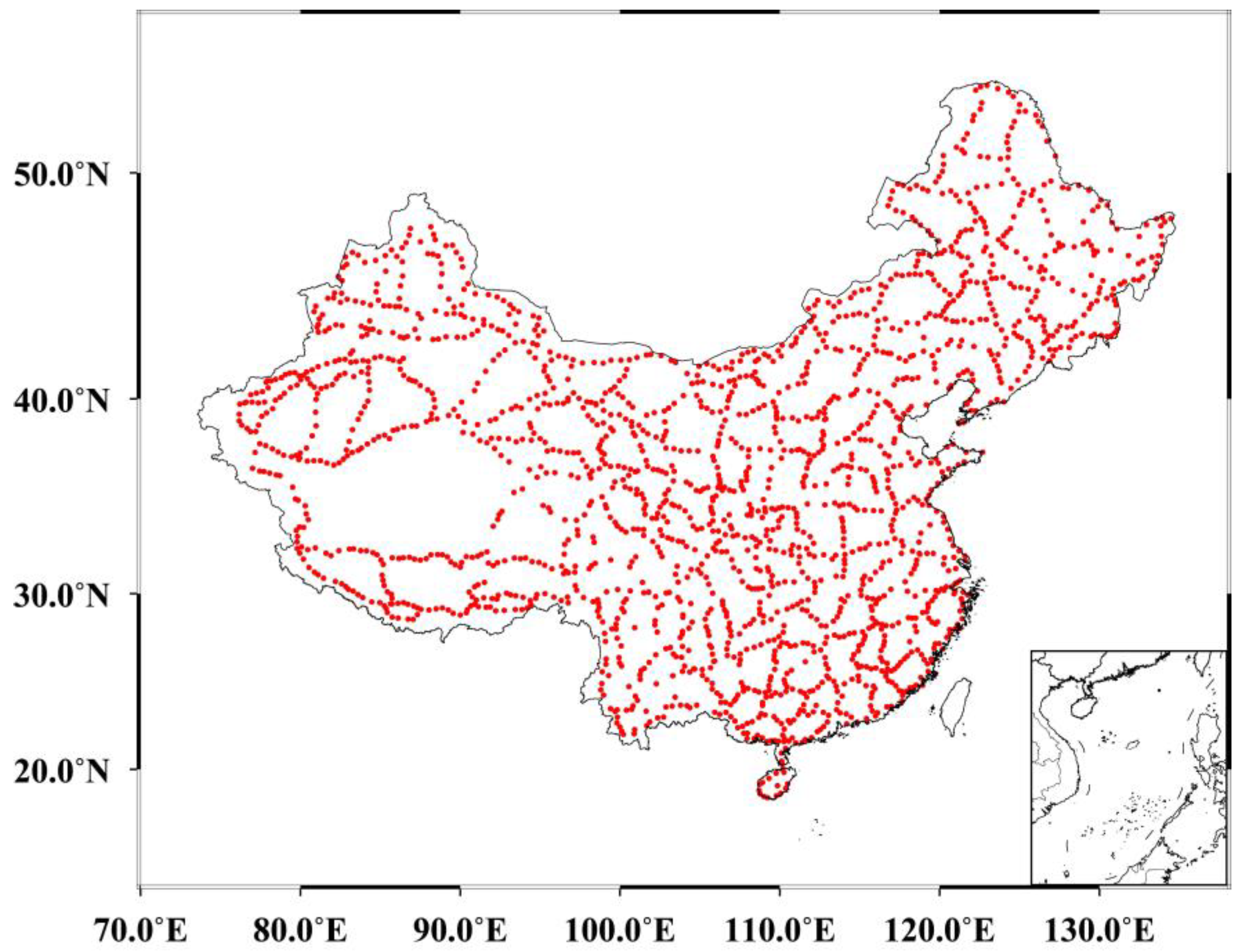
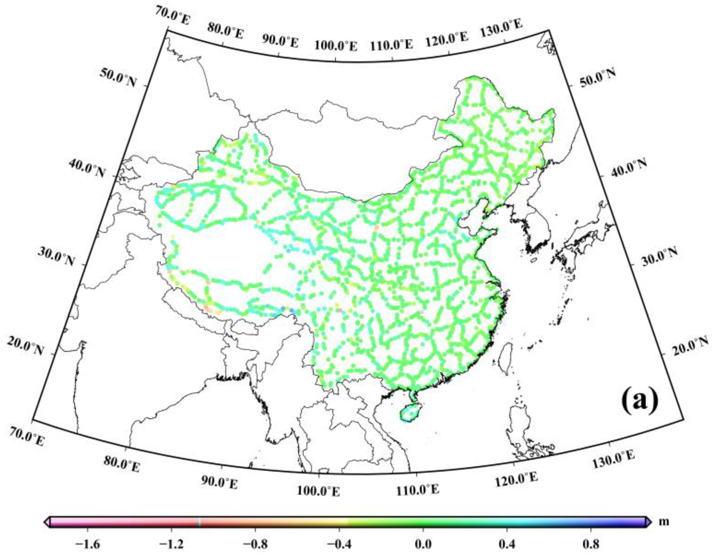
2.1.1. GNSS/LEVELING Data

The leveling networks in China contain the first-, second-, third-, and fourth-order leveling networks. The latest first-order leveling network observations, which were completed and placed into use in 2017, are used. This first-order leveling network consists of 148 loops with a length of over 125,746.5 km. Considering the large east–west span in China, the systematic accumulated error may occur in the long-distance leveling; therefore, the leveling data is handled by the least square adjustment in which the length correction of leveling rod, the non-parallel correction of level surface, and the gravity reduction are considered [32]. The maximum error in leveling is only about 3.57 cm (about 6185 km from Qingdao leveling origin) after adjustment. Finally, 1908 high-accuracy and evenly distributed GNSS/leveling datapoints are made available by the National Geomatics Center of China to determine the vertical datum geopotential of China. The GNSS ellipsoidal coordinates are based on ITRF2014 [38], and the GNSS coordinate accuracy reaches the millimeter level; in particular, the accuracy of GNSS ellipsoidal heights is about 5 mm. The distribution for the GNSS/leveling datapoints in China is shown in Figure 1.
Because the GNSS ellipsoidal height is based on a tide-free system, to ensure that the GNSS/leveling-based quasi-geoid height represents a tide-free system, the normal heights are transformed to the tide-free system by the following equation [39]:
H T F = H M F + 0.68 ( 0.099 0.296 sin 2 φ )
where HTF represents the tide-free normal height, HMF is the mean tide normal height, and φ is the latitude of the GNSS/leveling points.

2.1.2. Global Gravity Field Models (GFMs)

Table 1 shows the GFMs used in this paper. The direct approach is employed to derive the DIR_R5 and DIR_R6 models using GOCE satellite gravity observations, GRACE satellite gravity observations, and satellite laser ranging (SLR). The DIR_R5 model utilizes GOCE data from November 2009–October 2013 and GRACE data from the ten-year period (2003–2012). The DIR_R6 model utilizes GOCE data from October 2009–October 2013 and GRACE data from January 2007–November 2014. The TIM_R5 and TIM_R6 models are derived by the time-wise approach using GOCE observations from November 2009–October 2013 and September 2009–October 2013, respectively. The EGM2008 model combines multi-source gravity observation data to derive a maximum degree of 2190; however, this model is complete to d/o 2159. The gravity data utilized in EGM2008 model mainly refers to global gravity database of 5′ × 5′. The surface gravity data covering China is composed of two-divisions: one is the gravity data of 5′ for construction of the EGM2008, without any restrictions, the main coverage areas include eastern, southern, and Central China; another gravity data resource is permitted to use at a resolution of 15 arc-minute, these data cover other regions except for eastern, southern, and Central China.
For the consistency of tide system, the C ¯ 20 coefficient of GFM is transformed to tide-free system using the following formula [40]:
C ¯ 20 T F = C ¯ 20 Z T k 20 Δ C ¯ 20
where C ¯ 20 T F and C ¯ 20 Z T are the spherical harmonic coefficient under the tide-free system and the zero-tide system, respectively, k 20 = 0.30190 is loading Love number, and Δ C ¯ 20 = 1 . 391412 10 8 represents the value of tidal correction.
Table 1. The details for global gravity field models. The letter “S” in the third column represents satellite data, “G” represents ground observations, “A” represents altimetry observations, and “d/o” represents degree/order.
Modelsd/oDataTide SystemReference
EGM20082160S(Grace), G, ATide-free[41]
GO_CONS_GCF_2_TIM_R5280S(Goce)Tide-free[42]
GO_CONS_GCF_2_TIM_R6300S(Goce)Zero-Tide[43]
GO_CONS_GCF_2_DIR_R5300S(Goce, Grace, Lageos)Tide-free[44]
GO_CONS_GCF_2_DIR_R6300S(Goce, Grace, Lageos)Tide-free[45]

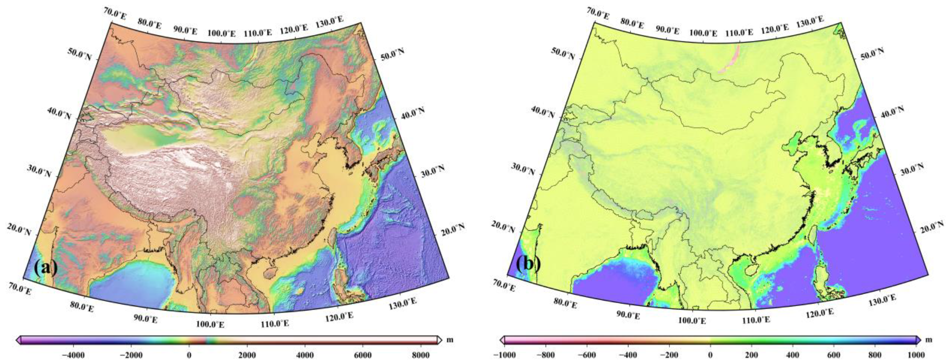
2.1.3. Topographic Data

Topographic data are used to calculate the RTM effect and recover the high-frequency gravity signals missing in the GFMs. The RTM represents the difference between the topographic surface and the long-wavelength reference terrain. The Shuttle Radar Topographic Mission (SRTM) V4.1 data [46] with a spatial resolution of 7.5″ × 7.5″ are used to represent the land over China. For the sea area, the SRTM15_PLUS V2 topographic data [47] are used, with a spatial resolution of 15″ × 15″. The rock-equivalent topography model RET2012 [48] works as the reference topography, and the reference terrain elevations can be computed by Equation (2) in [49]. In the coastal zone, the mass density of seawater is different from that of the standard topographic mass density. To avoid the necessity of distinguishing density changes in the computational process, the rock-equivalent topography (RET) method can be used to compress the water depth to the equivalent rock height [50].
H = H ( 1 ρ w / ρ )
where H and H are the compressed water depth and the original water depth, respectively, ρ w denotes the density of seawater, and ρ represents the standard topographic mass density.
The SRTM and SRTM15_PLUS data can be merged to obtain the unified topographic data on land and sea. The merging process is mainly divided into two steps: (1) the bicubic interpolation method is employed to interpolate the sea topographic data into a spatial resolution of 7.5″ × 7.5″, and Equation (3) is employed to process the sea water depths; (2) the land topographic data are combined with the water depth data obtained by step (1). Figure 2a shows the merged topography. The residual topographic masses (RTM elevations) are the difference between the SRTM merged data (Figure 2a) and the reference terrain. Figure 2b shows the residual terrain model elevations.

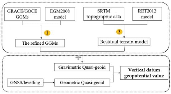
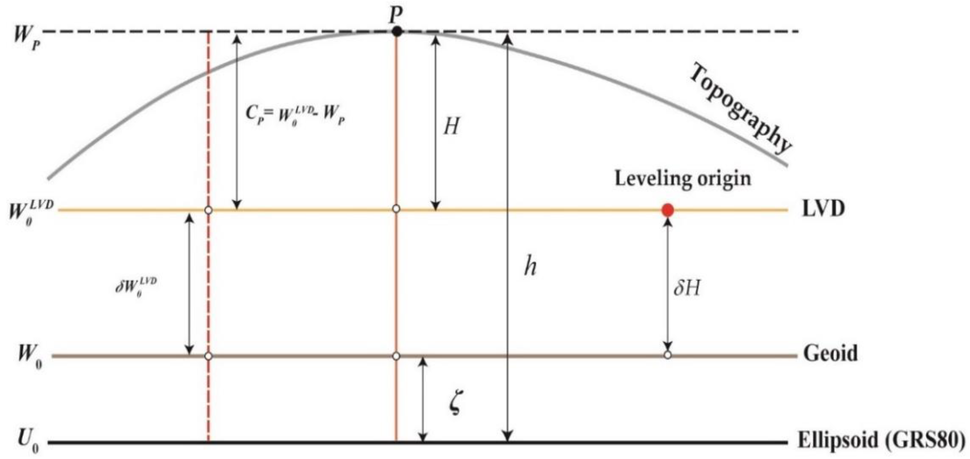
2.2. Methods for Determining the Height Datum Geopotential Value

The vertical offset δ H between the local height datum and the global geoid can be expressed as
δ H = h H ζ
where H represents the normal heights, h is the ellipsoidal heights, and ζ is the height anomalies from GFM (see Figure 3).
The height anomaly ζ can be calculated by using the satellite-only GFMs, but the resulting omission errors cannot be ignored. Therefore, the EGM2008 model can be used to extend the satellite-only GFMs to obtain the refined GFMs via the spectral expansion approach. The height anomaly ζ G G M determined by the refined GFMs can be expressed as
ζ G G M = ( G M G M 0 r γ ¯ W 0 U 0 γ ¯ ) + ζ G O C E / G R A C E | 2 l + ζ E G M 2008 | l + 1 2160
where ζ G O C E / G R A C E | 2 l is the height anomaly determined by the satellite-only GFMs truncated to the degree l, and ζ E G M 2008 | l + 1 2160 is the height anomaly represented from degrees 201 to 2160 of EGM2008. GM0 = 3.986005000 × 10¹⁴ m3s−2 and U0 = 62,636,860.8500 m2s−2 are constants of the gravitational constant and the normal potential value of the GRS80 ellipsoid [51], respectively; r is the geocentric radial for computation point; GM represents geocentric gravitational constant used in the GFM; γ ¯ is the mean normal gravity; and W0 = 62,636,853.4 m2s−2 is the geopotential value of the global geoid [52].
The RTM technology is used to recover the short-scale signal beyond degree 2160 in Equation (5). The RTM represents the difference (residual terrains) between the topographic surface and the reference surface. The gravitational potentials of residual terrains can be expressed as follows [53]:
T = G ρ Ω 1 r d Ω
where T is the gravitational effect for the residual terrains, G denotes the gravitational constant, r is the distance between the attraction mass and the computation point, Ω is the volume for the residual terrains, and ρ is the standard topographic mass density.
The residual terrains are decomposed into a set of rectangular-prism mass. Figure 4 shows the coordinate system definition of a rectangular-prism mass body. The computation point P is the origin of this coordinate system; this means that the coordinates defining have to be transformed by a shift (see Equation (1) in [54]). To obtain the gravitational effects of a residual mass distribution, the result of Equation (6) for a single rectangular-prism can be calculated using the following equation:
T ( P ) = G ρ x 1 x 2 y 1 y 2 z 1 z 2 1 r d x d y d z = G ρ | | | x y ln ( z + r ) + y z ln ( x + r ) + z x ln ( y + r ) x 2 2 tan 1 ( y z x r ) y 2 2 tan 1 ( x z y r ) z 2 2 tan 1 ( x z z r ) | x 1 x 2 | y 1 y 2 | z 1 z 2
where x1, x2, y1, y2, z1, and z2 describe the corner coordinates of the prism faces in Figure 4.
The total gravitational effects of the residual terrains for computation point are derived by a summation of gravitational effects in Equation (7):
T ( P ) = i = 1 M T ( P ) i
where M represents the number for prism mass elements.
The height anomaly ζ R T M caused by the residual mass distribution can be expressed by
ζ R T M = T ( P ) γ P
where γ P is normal gravity for computation point P.
ζ R T M represents the quasi-geoid height signals of the GFM beyond degree 2160. Then, the height anomaly ζ determined by the refined GFMs can be further expressed as follows:
ζ = ζ G G M + ζ R T M = ( G M G M 0 r γ ¯ W 0 U 0 γ ¯ ) + ζ G O C E / G R A C E | 2 l + ζ E G M 2008 | l + 1 2160 + ζ R T M
The global or local vertical datum is a gravitational equipotential surface. Therefore, the vertical datum offset determined by Equation (4) should theoretically be a fixed constant. However, vertical offsets contain certain discrepancies due to the influences of systematic errors and random errors. Systematic errors may contain possible systematic errors in GFM, accumulated leveling errors and the GNSS height ellipsoidal errors [55,56,57]. To reduce these random and systematic errors, the vertical datum offset is estimated by applying a planar correction parametric model. For each GNSS/leveling point P, the observation equation can be formulated as follows:
l P = h P H P ζ P = δ H ¯ + a 1 ( B P B 0 ) + a 2 ( L P L 0 ) cos B P
where δ H ¯ is the unknown height datum offset, ( B P , L P ) are the geodetic coordinates for the computation point, ( B 0 , L 0 ) are the geodetic coordinates for leveling origin in the local vertical datum zone, and a1 and a2 are the north–south tilt and east–west tilt, respectively. If there are n GNSS/leveling benchmarks in the local vertical datum zone, according to Equation (11), the function model can be expressed as follows:
[ h 1 H 1 ζ 1 h 2 H 2 ζ 2 h n H n ζ n ] l = [ 1 ( B 1 B 0 ) ( L 1 L 0 ) cos B 1 1 ( B 2 B 0 ) ( L 2 L 0 ) cos B 2 1 ( B n B 0 ) ( L n L 0 ) cos B n ] A [ δ H ¯ a 1 a 2 ] x
The unknown parameter x in Equation (12) can be further determined according to the least square adjustment of the system, denoted by
x = ( A T P A ) 1 A T P l
where P = D l l 1 is the weight matrix, D l l represents the error variance–covariance matrix for the observed values. Assuming the involved terms in Equation (11) are uncorrelated to each other, the D l l can be specified by
D l l = D h h + D H H + D ζ ζ
where D h h and D H H are the error variance–covariance matrix of the ellipsoidal and normal heights, respectively, and D ζ ζ represents the error variance–covariance matrix for quasi-geoid heights.
D ζ ζ might be determined from the errors of the GFMs and RTM quasi-geoid heights. Voigt and Denker [58] and Grombein et al. [17] showed that the uncertainty of the topography-implied gravity signals is at the sub-mm level; therefore, the errors of RTM quasi-geoid heights can be considered negligible. However, the error variance–covariance matrix of the GFM might generally not be available [17]. In addition, the uncertainties for ellipsoidal heights and normal heights are usually not available. Therefore, it is not possible to obtain D l l in practical cases. Based on the above reasons, we assume P = I in this paper, where I is the identity weight matrix.
After removing the errors effects, we will obtain vertical offsets with considering corrections by
δ H P = ( h P H P ζ P ) a 1 ( B P B 0 ) a 2 ( L P L 0 ) cos B P
The geopotential value W P 0 L V D for point P can be expressed as follows:
W P 0 L V D = W 0 δ H P γ ¯ P
where γ ¯ P denotes the mean normal gravity, which is computed by Equations (4)–(60) in [59].
Finally, we can derive the geopotential value W 0 L V D of the local height datum by
W 0 L V D = W 0 P = 1 m δ H P γ ¯ P m = W 0 δ W 0 L V D
where m is the number of GNSS/leveling benchmarks.

3. Results

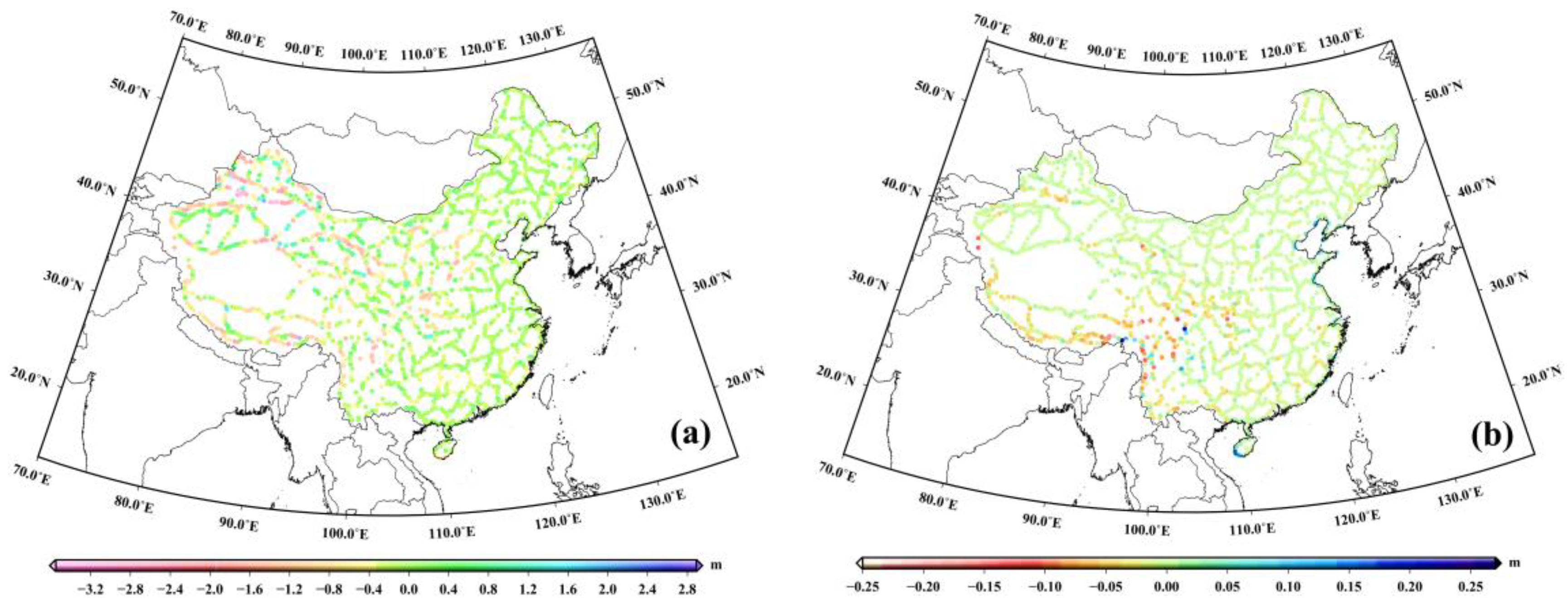
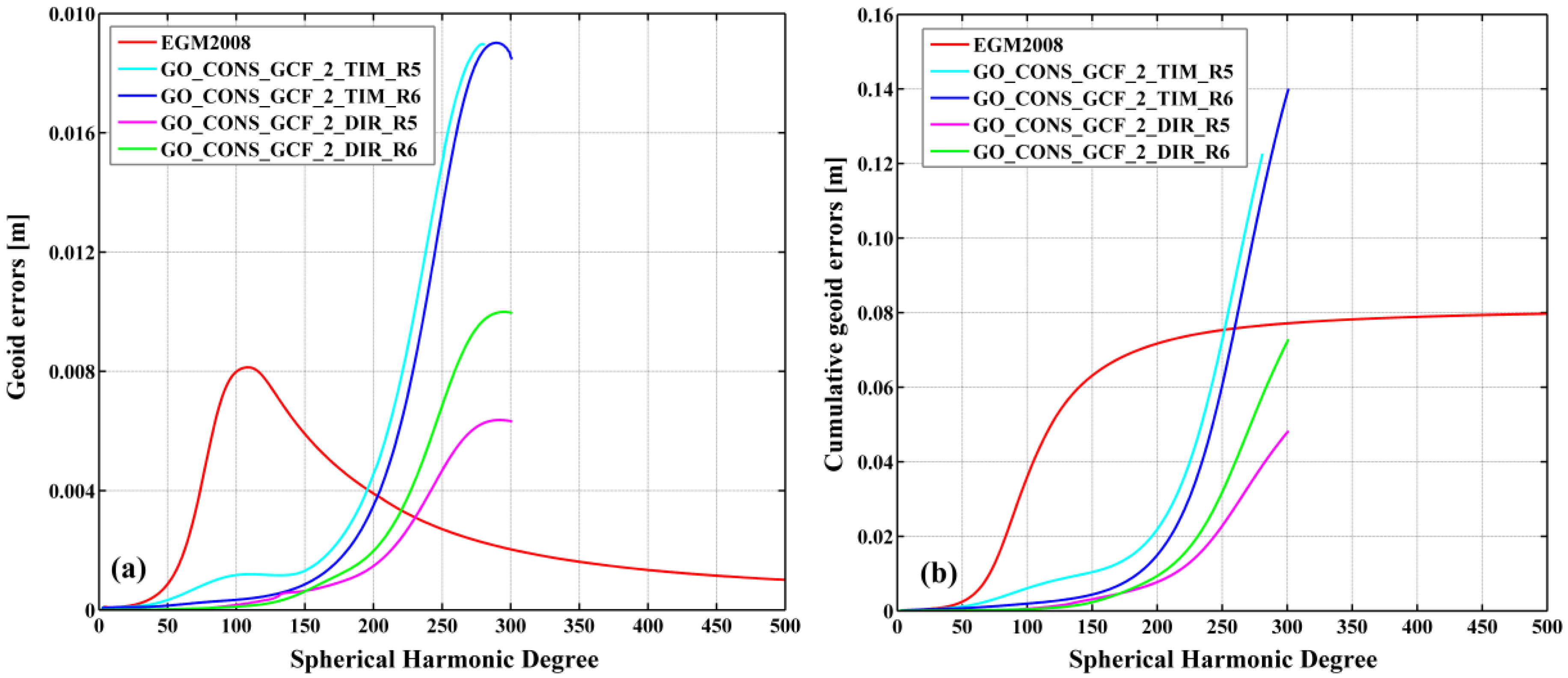
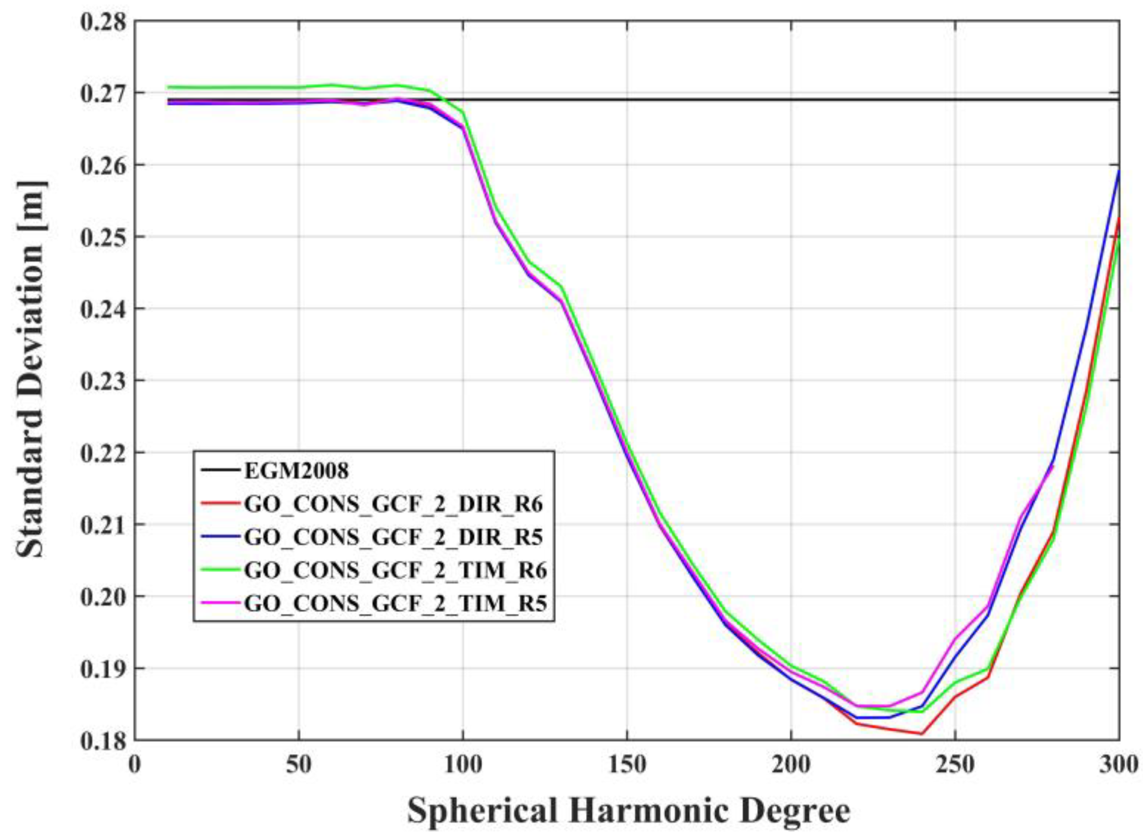
3.1. Spectral Accuracy Evaluation for GFMs

According to the spherical harmonic coefficients and their formal errors, the spectral accuracy of a GFM is evaluated by using the commission errors (the degree error, cumulative degree error, difference degree error, and cumulative difference degree error) and signal-to-noise ratio (SNR). The geoid degree error can be expressed as the square root of the error degree variances, and the cumulative geoid degree error is represented as the square root of the cumulative geoid error degree variances. A relative comparison of satellite-based GFM and EGM2008 can be estimated by the difference degree error and the cumulative difference degree error. These specific calculation formulas can be found in [60].
Figure 5a shows the geoid degree errors for GFMs. We can see from the figure that the geoid degree errors of the satellite-only GFMs before about degree 200 are lower than the degree error of EGM2008. Figure 5b shows the geoid cumulative degree errors for the GFMs. The geoid cumulative degree errors for DIR_R5 and DIR_R6 models are lower than that of the EGM2008 model in the whole spectral domain. The geoid cumulative degree errors for TIM_R5 and TIM_R6 models are lower than that of the EGM2008 model before approximately degree 260. The above analysis shows that the satellite-only GFMs have higher medium–long wavelength accuracy than the EGM2008 model, and the satellite-based GFMs are characterized by noise as increases in degree.
Figure 6a indicates the SNRs for the GFMs. The SNRs of satellite-only GFMs are better than that of the EGM2008 model before about degree 200. The results show that the satellite-only GFMs have a strong geoid signal in the medium–long wavelength band, and the EGM2008 model has a strong geoid signal in the short wavelength band. Figure 6b shows the difference degree error and cumulative difference degree error of the satellite-only GFMs, taking the EGM2008 model as a reference. We can see from the figure that the geoid difference degree errors for DIR_R5 and DIR_R6 are lower than geoid difference degree errors of the TIM_R5 and TIM_R6 before about degree 100, and cumulative geoid difference degree errors of the DIR_R5 and DIR_R6 are lower than cumulative difference degree errors of TIM_R5 and TIM_R6 before about degree 150. This is because the DIR_R5 and DIR_R6 GFM take advantage of GRACE gravity data and LAGEOS satellite laser ranging (SLR) data.

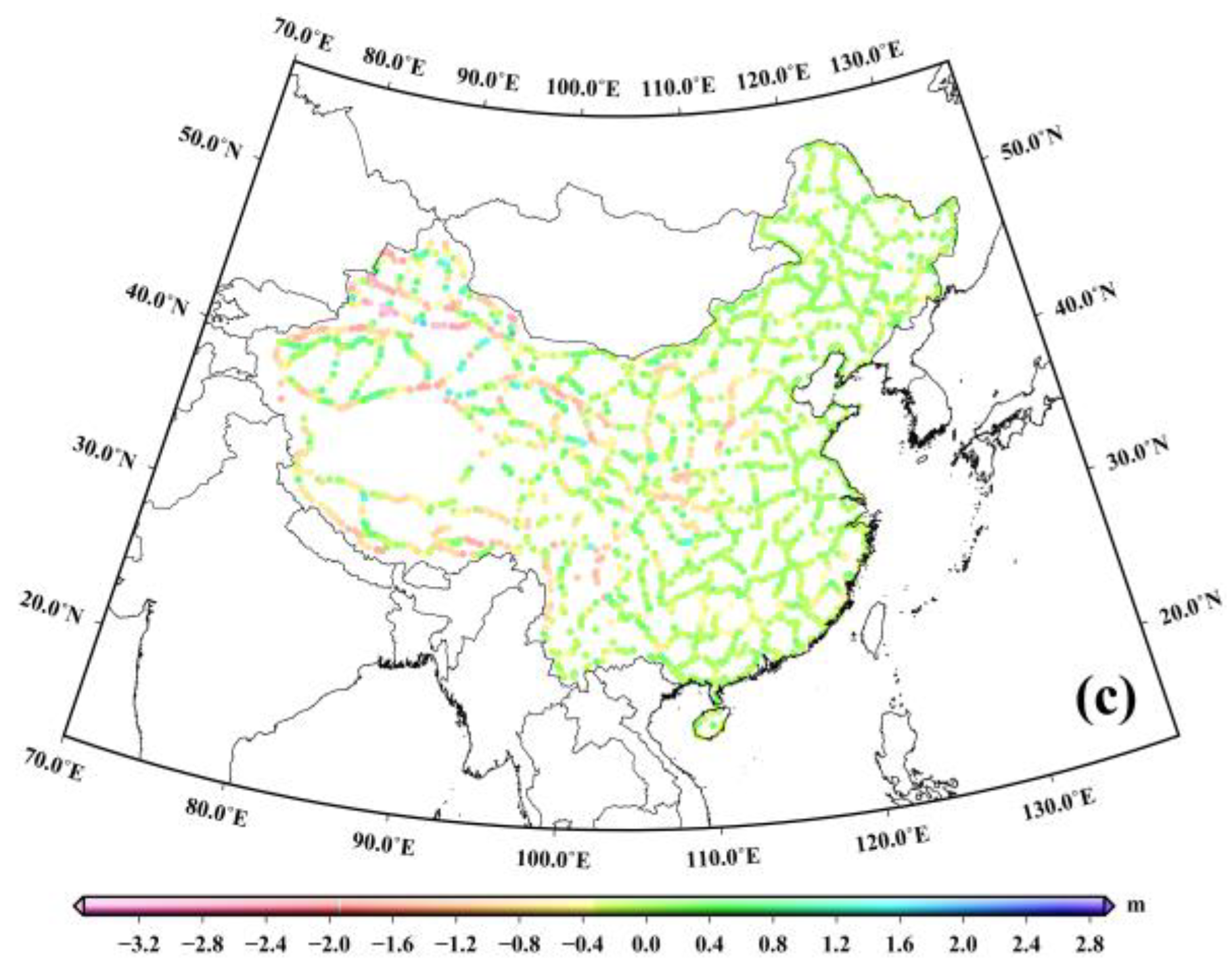
3.2. The Omission Errors for Satellite-Only GFMs

To quantify the magnitudes of these omission errors of satellite-only GFMs, we assume that 200 is the general expansion degree of the satellite-only GFM. The magnitudes of the height anomaly ζ 201 - 2160 E G M 2008 using the degrees 201 to 2160 of EGM2008 and the height anomaly ζ R T M inferred from the RTM can indicate the omission errors of the satellite-only GFM. The specific calculation process for ζ R T M can be found in Section 3.3.
Figure 7a indicates the omission error of satellite-only GFM represented by ζ 201 - 2160 E G M 2008 , Figure 7b shows the omission errors of satellite-only GFM represented by the ζ R T M , and Figure 7c shows the total omission errors obtained from the sum of ζ 201 - 2160 E G M 2008 and ζ R T M . Table 2 show statistics for the omission errors of satellite-only GFM in China. We can see from the figure that the omission errors in the rugged regions are larger (mid-west of mainland China) than in other regions. From Table 2, we can see that the omission errors of the satellite-only GFM in mainland China reach the decimeter level, and the largest amplitude is about 350 cm. The omission error signals represented by the RTM are centimeter level in mainland China. Therefore, the omission errors for the satellite-only GFMs must be considered for unification of China vertical datum.

3.3. The Refined GFMs Obtained by the Spectral Expansion Approach

A spectral expansion approach is used to obtain the refined gravity field models using the EGM2008 (Earth Gravitational Model 2008) and residual terrain model (RTM) technique. Because the degree errors of the satellite-only GFMs increase with the increase in degree and order, the noise starts to dominate the signals at high degree and order. Therefore, it is not possible to derive an optimal GFM by combining the maximum degree of satellite-based GFMs and EGM2008. It is not a reasonable strategy to obtain a refined GFM by combining two models directly, and the choice of the optimal degree for the combination is very important. The specific steps used to determine the optimal combination degrees are as follows: (a) the satellite-only GFMs are truncated to degree l (l = 10, 20, 30……N, where N is the maximum degree for satellite-only GFMs) as the 0~l degree of the refined GFMs, and the l~2160 degree of the refined GMFs is supplemented by the corresponding degree of the EGM2008 model; (b) the GNSS/leveling-based height anomaly is used to check the height anomaly determined by the refined GFMs; (c) the combination degree presenting the best accuracy is chosen as the optimal combination degree of the refined GFMs. Figure 8 indicates the standard deviations of the height anomalies differences between GNSS/leveling and the refined GFMs with varying combinations of degree. As seen in Figure 8, the accuracy of the combined GFMs is basically consistent with that of the EGM2008 model before about degree 90. From degree 90 onwards, there are obvious differences in accuracy. We select the optimal combination degree when the standard deviations minimized. Figure 8 shows that 230, 240, 220, and 240 are the optimal combination degrees for obtaining the refined GFMs by combining the TIM_R5, TIM_R6, DIR_R5, and DIR_R6 models, respectively, with the EGM2008 model.
The RTM technology can further be utilized to obtain higher frequency gravity field signals of the refined GFMs. The RTM gravitational potential is not harmonic when the computation point is below the reference elevation surface. In order to solve the problem of non-harmonic, a harmonic correction can usually be performed by downward continuation through a Bouguer plate [33,61]. Thus, the harmonic correction for quasi-geoid (or geoid) can be considered as zero; however, harmonic correction for gravity can be considered as 4 π G ρ Δ H ( Δ H represents the height difference between the topography and reference terrain). The choice of the RTM integration radius is crucial. For RTM quasi-geoid height, an integration radius of ~200 km is suitable [49]. Therefore, an integration radius of ~200 km is used herein to determine the RTM quasi-geoid heights. According to unified topographic data (in Figure 2), we can obtain RTM quasi-geoid height by using Equations (7)–(9). Figure 9 shows the quasi-geoid contribution of the RTM with a resolution of 7.5” × 7.5”, with maximum, minimum, mean, and standard deviation values of 0.301 m, −0.280 m, 0.001 m, and 0.020 m, respectively.
Table 3 shows the quasi-geoid accuracy statistics of different GFMs in China. From Table 3, without considering the influence of the RTM on the quasi-geoid height, the quasi-geoid accuracies of the refined GFMs in mainland China are better than 18.5 cm. Among them, the DIR_R6_EGM2008 model has the best accuracy, at 18.1 cm. Compared with the EGM2008 model, the quasi-geoid accuracy of the DIR_R6_EGM2008 model is improved by 8.8 cm. On the other hand, these results also indicate that the quasi-geoid medium-long wavelength accuracy of EGM2008 model in China is poor. Considering the influence of the RTM quasi-geoid, the mainland China quasi-geoid accuracies determined by the refined GFMs are better than 17.8 cm, and the DIR_R6_EGM2008_RTM model has the optimal quasi-geoid accuracy with a standard deviation of 17.3 cm. Compared with the EGM2008 model, the quasi-geoid accuracy of the DIR_R6_EGM2008_RTM model is improved by 9.6 cm. Compared with the TIM_R5, TIM_R6, DIR_R5, and DIR_R6 models, the quasi-geoid accuracy of the DIR_R6_EGM2008_RTM model is improved by 0.400 m, 0.391 m, 0.396 m, and 0.391 m to 0.178 m, 0.177 m, 0.176 m, and 0.173 m, respectively.
To validate our results of the refined GFMs, the EIGEN-6C4 [62], GECO [63], SGG-UGM-1 [64], SGG-UGM-2 [65], XGM2016 [66], and XGM2019 [67] models are used. These six higher-degree GFMs further improve the medium–long wavelength by adding GOCE data.
Table 4 summarizes the statistics for height anomaly differences between GNSS/leveling and six higher-degree GFMs. These models in Table 4 perform better than the EGM2008 model in China, which can assume the largest impact from the contribution of GOCE solution. The EIGEN-6C4 outperforms GECO, SGG-UGM-1, and SGG-UGM-2 models in China, which is mainly due to the differences in use of GOCE data. Comparing Table 3 and Table 4, we can find that the refined GFMs outperform EIGEN-6C4, GECO, SGG-UGM-1, XGM2019, XGM2016, and SGG-UGM-2 in mainland China; the major improvement of these models can be attributed to the GOCE data and topography signals.

3.4. Determination for the Geopotential Value of Chinese Height Datum

The geopotential W0 = 62,636,853.4 m2s−2 adopted as reference level for the IHRS is used herein. Based on the GFM, the vertical datum geopotential value for China is determined. Thus, the vertical datum in China is connected into the IHRS.
In the analysis presented in Section 3.3, we conclude that the DIR_R6_EGM2008_RTM model has optimal quasi-geoid accuracy in China. Therefore, we choose this model to derive the Chinese height datum geopotential value. According to Equation (4), we can obtain vertical offset values of each GNSS/leveling point. Figure 10a represents the height anomaly differences between the GNSS/leveling and the DIR_R6_EGM2008_RTM model in China, thus providing the spatial distribution for the vertical datum offsets. However, it can be found from Figure 10a that the discrepancies exist in mainland China. The vertical offsets have certain discrepancies due to the influence of various factors. Among them, systematic error is a major contributor. Therefore, the planar corrections surface is used further through Equation (11). Then, we can derive vertical offsets after applying the correction surfaces by Equation (15). Figure 10b shows correction surface at GNSS-leveling points. Figure 10c shows vertical offsets after applying the correction surfaces. It can be seen from Figure 10b that there are certain east–west systematic errors in China, and the maximum error is about 12.2 cm. Systematic errors mainly contain errors in the GFM and leveling, The maximum first-order leveling error in China is only about 3.57 cm after height networks adjustment [32]. Therefore, we can conclude that the major systematic effect contributor to the estimation of the height datum geopotential values of China mainly comes from GFM error, and the systematic errors from GFM are more obvious in western China.
The systematic errors influence on the determination of the Chinese height datum geopotential values is evaluated. The results with and without consideration of systematic error effect are compared, as shown in Table 5. Table 5 presents the numerical results of both scenarios based on the DIR_R6_EGM2008_RTM model. As shown in Table 5, we can see that there is a minor improvement of 0.06 m2s−2 for DIR_R6_EGM2008_RTM model when considering the planar corrections. Finally, the geopotential value for the Chinese height datum is derived to be equal to 62,636,853.29 m2s−2 based on the DIR_R6_EGM2008_RTM model, considering planar corrections.

4. Discussion

The satellite-only GFMs have high spectral accuracy and strong geoid signals. How-ever, the maximum expansion degree of these satellite-based models is limited and there are certain omission errors as a result of the gravity field attenuation at the height of satellite orbit. From Figure 7 and Table 2, we can see that the omission errors of the satellite-only GFM in mainland China reach the decimeter level, and the largest amplitude is about 350 cm. The omission error signals represented by the RTM are centimeter level in mainland China. Therefore, the omission errors for the satellite-only GFMs must be considered for unification of China vertical datum. The satellite-only GFMs have higher spectral accuracy and stronger geoid signals at medium–long wavelength, and EGM2008 model has stronger geoid signals at short wavelength. Therefore, combining the GRACE/GOCE-based GFMs and EGM2008 model to obtain refined GFMs is a feasible strategy.
We combine the GRACE/GOCE-based GFMs and EGM2008 model to derived refined GFMs. The accuracy trend of the refined GFMs in Figure 8 mainly depends on the EGM008 model, the satellite-only GFMs, and GNSS/leveling resources. The GNSS/leveling have a good accuracy and quality; especially, the systematic errors in leveling have been greatly weakened by height network adjustment. Therefore, the results presented in Figure 8 mainly reflect the accuracy of the combined GFMs in China. The accuracy of the combined GFMs relies heavily on the improvement of the satellite-only models. Gruber and Willberg [56] demonstrated that 80% accuracy improvement for high-resolution GFMs compared with EGM2008 reveal the contribution of GOCE solution to medium wavelengths. Therefore, high-quality GNSS/leveling resources and the satellite-only GFMs increase the quality and reliability of the combined GFMs in this study. In the combination process, the satellite-only GFM using GOCE, GRACE, and LAGEOS laser ranging data should be used, which can better meet the quasi-geoid medium–long wavelength signal.
The RTM technology can further be utilized to obtain higher-frequency gravity field signals of the refined GFMs. In the spectral expansion process, the spatial resolution of the refined GFMs obtained by combining the satellite-only GFMs and EGM2008 model is 5′. Because the RET2012 reference topographic model has the same resolution as the refined GFMs, the reference model serves as a high-pass filter that can filter out low-frequency features from the SRTM data. As a result, the residual terrain height can imply gravity field signals at shorter scales than the spatial resolution of the refined GFMs and further compensate for the omission error of the refined GFMs. It can be seen from Figure 9 that larger quasi-geoid signals are strongly correlated with topography. However, it should be noted that the RTM quasi-geoid signals may contain some possible implications due to density anomaly and the uncertainties in the harmonic correction [48].
Finally, we use the refined GFMs to preliminarily derive the geopotential value of the Chinese height datum by utilizing the latest normal height results. The refined GGMs provide obvious accuracy improvement advantage and provide guidance for developing a high-accuracy quasi-geoid in China. Prior to this work, He et al. [20] determined the geopotential value of China’s height datum as 62,636,853.47 m2s−2, which fits well with our value of 62,636,853.29 m2s−2, considering the standard deviation. The geopotential value of Chinese height datum is determined by utilizing the latest national first-order leveling network and GNSS points in this paper, which are representative to some extent.
We can expect that the refined GFMs can provide a guidance for determining the quasi-geoid or the geopotential value of the Chinese height datum. However, the combination of the satellite-only GFM with the EGM2008 in this study is by a pure complementation of the spherical harmonic coefficients at a specific degree; however, such a procedure might cause a spectral gap between both models, which is different from rigorous combination that is carried out on the basis of the normal equations and covariance by a least-squares. In the next step, the rigorous combination will be considered to derive the refined GFMs. In addition, the well-distributed surface gravity data for determining the geopotential value of the Chinese height datum also play a crucial role and need to be considered further.

5. Conclusions

In this paper, we used a spectral expansion to derive the refined GFMs by combining the EGM2008 and the satellite-only GFMs. The results show that 230, 240, 220, and 240 are the optimal combination degrees for determining the refined GFMs by combining the TIM_R5, TIM _R6, DIR_R5, and DIR_R6 models with the EGM2008 model, respectively. To consider the influence of higher-frequency gravity field signals caused by topography, the RTM is utilized to further compensate for the omission errors in the refined GFMs. The mainland China quasi-geoid accuracies determined by the refined GFMs are better than 17.8 cm, and the DIR_R6_EGM2008_RTM model has an optimal quasi-geoid accuracy with of 17.3 cm. To validate our results of the refined GFMs, the EIGEN-6C4, GECO, SGG-UGM-1, and SGG-UGM-2, XGM2019, and XGM2016 models were used. The results show that the refined GFMs outperform EIGEN-6C4, GECO, SGG-UGM-1, XGM2019, XGM2016, and SGG-UGM-2 in mainland China; the major improvement of these models can be attributed to the GOCE data and topography signals.
The systematic error effects for determining the geopotential value of the Chinese height datum are considered. The results show that the refined GFMs show minor improvements when considering the planar corrections. The major systematic effect contributor for determining the Chinese height datum geopotential values mainly comes from GFM error. Finally, the Chinese height datum geopotential value is derived to be equal to 62,636,853.29 m2s−2 based on the refined DIR_R6_EGM2008_RTM model when considering planar corrections.

Author Contributions

Conceptualization, P.Z. (Panpan Zhang) and L.B.; methodology, P.Z. (Panpan Zhang) and L.B.; software, P.Z. (Panpan Zhang) and Z.L.; validation, P.Z. (Panpan Zhang); formal analysis, P.Z. (Panpan Zhang) and L.B.; investigation, all; resources, Z.L.; writing—original draft preparation, P.Z. (Panpan Zhang); writing—review and editing, L.B., Z.L. and L.W.; visualization, P.Z. (Panpan Zhang); supervision, L.W., L.B. and Z.L.; funding acquisition, L.B. and Z.L. All authors have read and agreed to the published version of the manuscript.

Funding

The research was funded by the National Natural Science Foundation of China (Grant Nos. 42174102, 42192535, and 41931076), the Project supported by the Open Fund of Hubei Luojia Laboratory, the Basic Frontier Science Research Program of Chinese Academy of Sciences (Grant No. ZDBS-LY-DQC028), and the National Key Research and Development Program of China (Grant No. 2016YFB0501405).

Institutional Review Board Statement

Not applicable.

Informed Consent Statement

Not applicable.

Data Availability Statement

The global Earth Models can be downloaded from ICGEMs (http://icgem.gfz-potsdam.de/tom_longtime/, accessed on 30 April 2021) and SRTM data can be derived from NASA (https:/srtm.csi.cgiar.org/, accessed on 20 April 2021). In addition, the GNSS/leveling data can be obtained request up on the author.

Acknowledgments

We would thank the International Centre for Global Earth Models and NASA Shuttle Radar Topographic Mission for providing us with the GFMs and the digital terrain model data, respectively.

Conflicts of Interest

The authors declare no conflict of interest.

References

  1. Barzaghi, R.; De Gaetani, C.I.; Betti, B. The worldwide physical height datum project. Rend. Fis. Acc. Lincei. 2020, 31, 27–34. [Google Scholar] [CrossRef]
  2. Sánchez, L.; Ågren, J.; Huang, J.; Wang, Y.M.; Mäkinen, J.; Denker, H.; Ihde, J.; Abd-Elmotaal, H.; Ahlgren, K.; Amos, M.; et al. Advances in the realisation of the International Height Reference System. In Proceedings of the IUGG General Assembly, Rio de Janeiro, Brazil, 12–14 November 2019. [Google Scholar]
  3. Sánchez, L.; Barzaghi, R. Activities and plans of the GGOS Focus Area Unified Height System. In Proceedings of the IUGG XXVII General Assembly, Montreal, QC, Canada, 14 July 2019. [Google Scholar]
  4. Drewes, H. Reference Systems, Reference Frames, and the Geodetic Datum-Basic Considerations. In Observing Our Changing Earth; Sideris, M.G., Ed.; Springer: Perugia, Italy, 2009; Volume 133, pp. 3–9. [Google Scholar]
  5. Drewes, H.; Kuglitsch, F.l.; Adám, J.; Rózsa, S. The Geodesist’s Handbook 2016. J. Geod. 2016, 90, 907–1205. [Google Scholar] [CrossRef]
  6. Ihde, J.; Sánchez, L.; Barzaghi, R.; Drewes, H.; Foerste, C.; Gruber, T.; Liebsch, G.; Marti, U.; Pail, R.; Sideris, M. Definition and proposed realization of the international height reference system (IHRS). Surv. Geophys. 2017, 38, 549–570. [Google Scholar] [CrossRef]
  7. Sánchez, L.; Ågren, J.; Huang, J.; Wang, Y.M.; Mäkinen, J.; Pail, R.; Barzaghi, R.; Vergos, G.S.; Ahlgren, K.; Liu, Q. Strategy for the realisation of the International Height Reference System (IHRS). J. Geod. 2021, 95, 33. [Google Scholar] [CrossRef]
  8. Gerlach, C.; Rummel, R. Global height system unification with GOCE: A simulation study on the indirect bias term in the GBVP approach. J. Geod. 2013, 87, 57–67. [Google Scholar] [CrossRef]
  9. Amjadiparvar, B.; Rangelova, E.; Sideris, M.G. The GBVP approach for vertical datum unification: Recent results in North America. J. Geod. 2016, 90, 45–63. [Google Scholar] [CrossRef]
  10. Ophaug, V.; Gerlach, C. On the equivalence of spherical splines with least-squares collocation and stokes’s formula for regional geoid computation. J. Geod. 2017, 91, 1367–1382. [Google Scholar] [CrossRef]
  11. Sánchez, L.; Sideris, M.G. Vertical datum unification for the International Height Reference System (IHRS). Geophys. J. Int. 2017, 209, 570–586. [Google Scholar] [CrossRef]
  12. Ebadi, A.; Ardalan, A.; Karimi, R. The Iranian height datum offset from the GBVP solution and spirit-leveling/gravimetry data. J. Geod. 2019, 93, 1207–1225. [Google Scholar] [CrossRef]
  13. Zhang, P.; Bao, L.; Guo, D.; Wu, L.; Li, Q.; Liu, H.; Xue, Z.; Li, Z. Estimation of Vertical Datum Parameters Using the GBVP Approach Based on the Combined Global Geopotential Models. Remote Sens. 2020, 12, 4137. [Google Scholar] [CrossRef]
  14. Hayden, T.; Amjadiparvar, B.; Rangelova, E.; Sideris, M.G. Estimating Canadian vertical datum offsets using GNSS/levelling benchmark information and GOCE global geopotential models. J. Geod. Sci. 2012, 2, 257–269. [Google Scholar] [CrossRef] [Green Version]
  15. Gruber, T.; Gerlach, C.; Haagmans, R. Intercontinental height datum connection with GOCE and GPS-levelling data. J. Geod. Sci. 2012, 2, 270–280. [Google Scholar] [CrossRef]
  16. Gomez, M.E.; Pereira, R.A.D.; Ferreira, V.G.; Del Cogliano, D.; Luz, R.T.; de Freitas, S.R.C.; Farias, C.; Perdomo, R.; Tocho, C.; Lauria, E.; et al. Analysis of the Discrepancies between the Vertical Reference Frames of Argentina and Brazil. In IAG 150 Years; Rizos, C., Willis, P., Eds.; Springer International Publishing: Cham, Switzerland, 2015; Volume 143, pp. 289–295. [Google Scholar]
  17. Grombein, T.; Seitz, K.; Heck, B. On High-Frequency Topography-Implied Gravity Signals for a Height System Unification Using GOCE-based Global Geopotential Models. Surv. Geophys. 2016, 38, 443–477. [Google Scholar] [CrossRef]
  18. Li, J.; Chu, Y.; Xu, X. Determination of Vertical Datum Offset between the Regional and the global Height Datum. Acta Geod. Cartogr. Sin. 2017, 46, 1262–1273. [Google Scholar]
  19. Vergos, G.S.; Erol, B.; Natsiopoulos, D.A.; Grigoriadis, V.N.; Tziavos, I.N. Preliminary results of GOCE-based height system unification between Greece and turkey over marine and land areas. Acta. Geod. Geophys. 2018, 53, 61–79. [Google Scholar] [CrossRef]
  20. He, L.; Chu, Y.; Xu, X.; Zhang, T. Evaluation of the GRACE/GOCE Global Geopotential Model on estimation of the geopotential value for the China vertical datum of 1985. Chin. J. Geophys. 2019, 62, 2016–2026. [Google Scholar]
  21. Kelly, C.I.; Andam-Akorful, S.A.; Hancock, C.; Laari, P.; Ayer, J. Global gravity models and the Ghanaian Vertical Datum: Challenges of a proper definition. Surv. Rev. 2019, 53, 44–54. [Google Scholar] [CrossRef]
  22. Zhang, P.; Bao, L.; Guo, D.; Li, Q. Estimation of the height datum geopotential value of Hong Kong using the combined global geopotential models and GNSS/levelling data. Surv. Rev. 2021, 1–11. [Google Scholar] [CrossRef]
  23. Tapley, B.D.; Bettadpur, S.; Watkins, M.; Reigber, C. The gravity recovery and climate experiment: Mission overview and early results. Geophy. Res. Lett. 2004, 31, L09607. [Google Scholar] [CrossRef] [Green Version]
  24. Drinkwater, M.R.; Floberghagen, R.; Haagmans, R.; Muzi, D.; Popescu, A. GOCE: ESA’s first earth explorer core mission. In Earth Gravity Field from Space—From Sensors to Earth Science; Beutler, G., Ed.; Kluwer Academic Publishers: Bern, Switzerland, 2003; Volume 108, pp. 419–432. [Google Scholar]
  25. Hirt, C.; Gruber, T.; Featherstone, W.E. Evaluation of the first GOCE static gravity field models using terrestrial gravity, vertical defiections and EGM2008 quasigeoid heights. J. Geod. 2011, 85, 723–740. [Google Scholar] [CrossRef] [Green Version]
  26. Tziavos, I.N.; Vergos, G.S.; Grigoriadis, V.N.; Tzanou, E.A.; Natsiopoulos, D.A. Validation of GOCE/GRACE Satellite Only and Combined Global Geopotential Models over Greece in the Frame of the GOCESeaComb Project. In IAG 150 Years; Rizos, C., Willis, P., Eds.; Springer International Publishing: Cham, Switzerland, 2015; Volume 143, pp. 297–304. [Google Scholar]
  27. Gruber, T.; Visser, P.N.A.M.; Ackermann, C.; Hosse, M. Validation of GOCE gravity field models by means of orbit residuals and geoid comparisons. J. Geod. 2011, 85, 845–860. [Google Scholar] [CrossRef]
  28. Kaula, W.M. Theory of Satellite Geodesy; Blaisdell: Toronto, OH, USA, 1966. [Google Scholar]
  29. Forsberg, R. Modelling of the fine-structure of the geoid: Methods, data requirements and some results. Surv. Geophys. 1993, 14, 403–418. [Google Scholar] [CrossRef]
  30. Denker, H. Regional Gravity Field Modeling: Theory and Practical Results. In Sciences of Geodesy—II Innovations and Future Developments; Xu, G., Ed.; Springer: Heidelberg, Germany, 2013; pp. 185–291. [Google Scholar]
  31. Tscherning, C.C.; Rapp, R.H. Closed Covariance Expressions for Gravity Anomalies, Geoid Undulations, and Deflections of the Vertical Implied by Anomaly Degree Variance Models; Reports of the Department of Geodetic Science; The Ohio State University: Columbus, OH, USA, 1974. [Google Scholar]
  32. Wang, W.; Guo, C.; Li, D.; Zhao, H. Elevation change analysis of the national first order leveling points in recent 20 years. Acta Geod. Cartogr. Sin. 2019, 48, 1–8. [Google Scholar]
  33. Forsberg, R. A Study of Terrain Reductions, Density Anomalies and Geophysical Inversion Methods in Gravity Field Modelling; Scientific Report No.5; The Ohio State University: Columbus, OH, USA, 1984. [Google Scholar]
  34. Hirt, C.; Featherstone, W.E.; Marti, U. Combining EGM2008 and SRTM/DTM2006.0 residual terrain model data to improve quasigeoid computations in mountainous areas devoid of Gravity Data. J. Geod. 2010, 84, 557–567. [Google Scholar] [CrossRef] [Green Version]
  35. Yang, M.; Hirt, C.; Wu, B.; Deng, X.; Tsoulis, D.; Feng, W.; Wang, C.; Zhong, M. Residual Terrain Modelling: The Harmonic Correction for Geoid Heights. Surv. Geophys. 2022. [Google Scholar] [CrossRef]
  36. Hirt, C.; Bucha, B.; Yang, M.; Kuhn, M. A numerical study of residual terrain modelling (RTM) techniques and the harmonic correction using ultra-high degree spectral gravity modelling. J. Geod. 2019, 93, 1469–1486. [Google Scholar] [CrossRef]
  37. Yang, M.; Hirt, C.; Rexer, M.; Pail, P.; Yamazaki, D. The tree canopy effect in gravity forward modelling. Geophys. J. Int. 2019, 219, 271–289. [Google Scholar] [CrossRef]
  38. Altamimi, Z.; Rebischung, P.; Métivier, L.; Collilieux, X. ITRF2014: A new release of the International Terrestrial Reference Frame modeling nonlinear station motions. J. Geophys. Res. Solid Earth 2016, 121, 6109–6131. [Google Scholar] [CrossRef] [Green Version]
  39. Ekman, M. Impacts of geodynamic phenomena on systems for height and gravity. Bull. Géod. 1989, 63, 281–296. [Google Scholar] [CrossRef]
  40. Gruber, T.; Abrikosov, O.; Hugentobler, U. GOCE Standards. Prepared by the European GOCE Gravity Consortium EGG-C. 2014. Available online: https://earth.esa.int/documents/10174/1650485/GOCE_Standards (accessed on 1 June 2021).
  41. Pavlis, N.K.; Holmes, S.A.; Kenyon, S.C.; Factor, J.K. The development and evaluation of the earth gravitational model 2008(EGM2008). J. Geophys. Res. 2012, 117, B04406. [Google Scholar] [CrossRef] [Green Version]
  42. Brockmann, J.M.; Zehentner, N.; Höck, E.; Pail, R.; Loth, I.; Mayer-Gürr, T.; Schuh, W.-D. EGM_TIM_RL05: An independent geoid with centimeter accuracy purely based on the GOCE mission. Geophys. Res. Lett. 2014, 41, 8089–8099. [Google Scholar] [CrossRef]
  43. Brockmann, J.M.; Schubert, T.; Schuh, W.D. An Improved Model of the Earth’s Static Gravity Field Solely Derived from Reprocessed GOCE Data. Surv. Geophys. 2021, 42, 277–316. [Google Scholar] [CrossRef]
  44. Bruinsma, S.L.; Förste, C.; Abrikosov, O.; Lemoine, J.-M.; Marty, J.-C.; Mulet, S.; Rio, M.-H.; Bonvalot, S. ESA’s satellite-only gravity field model via the direct approach based on all GOCE data. Geophys. Res. Lett. 2014, 41, 7508–7514. [Google Scholar] [CrossRef] [Green Version]
  45. Förste, C.; Abrykosov, O.; Bruinsma, S.; Dahle, C.; König, R.; Lemoine, J.-M. ESA’s Release 6 GOCE Gravity Field Model by Means of the Direct Approach Based on Improved Filtering of the Reprocessed Gradients of the Entire Mission (GO_CONS_GCF_2_DIR_R6). Available online: https://doi.org/10.5880/ICGEM.2019.004 (accessed on 14 May 2021).
  46. Jarvis, A.; Reuter, H.I.; Nelson, A.; Guevara, E. Hole-Filled SRTM for the Globe Version 4. CGIAR-SXI SRTM 90 m Database. 2008. Available online: http://srtm.csi.cgiar.org (accessed on 14 April 2021).
  47. Tozer, B.; Sandwell, D.T.; Smith, W. Global Bathymetry and Topography at 15 Arc Sec: SRTM15+. Earth Space Sci. 2019, 6, 1847–1864. [Google Scholar] [CrossRef]
  48. Hirt, C.; Claessens, S.; Fecher, T.; Kuhn, M.; Pail, R.; Rexer, M. New ultrahigh-resolution picture of earth’s gravity field. Geophy. Res. Lett. 2013, 40, 4279–4283. [Google Scholar] [CrossRef] [Green Version]
  49. Hirt, C. RTM gravity forward-modeling using topography/bathymetry data to improve high-degree global geopotential models in the coastal zone. Mar. Geod. 2013, 36, 183–202. [Google Scholar] [CrossRef] [Green Version]
  50. Hirt, C.; Kuhn, M.; Featherstone, W.E.; Göttl, F. Topographic/isostatic evaluation of new-generation GOCE gravity field models. J. Geophys. Res. 2012, 117, B05407. [Google Scholar] [CrossRef] [Green Version]
  51. Moritz, H. Geodetic reference system 1980. J. Geod. 2000, 74, 128–133. [Google Scholar] [CrossRef]
  52. Sánchez, L.; Čunderlík, R.; Dayoub, N.; Mikula, K.; Minarechová, Z.; Šíma, Z.; Vatrt, V.; Vojtíšková, M. A conventional value for the geoid reference potential W0. J. Geod. 2016, 90, 815–835. [Google Scholar] [CrossRef]
  53. Yang, M.; Hirt, C.; Tenzer, R.; Pail, R. Experiences with the use of mass-density maps in residual gravity forward modelling. Stud. Geophys. Geod. 2018, 62, 596–623. [Google Scholar] [CrossRef]
  54. Nagy, D.; Papp, G.; Benedek, J. The gravitational potential and its derivatives for the prism. J. Geod. 2000, 74, 552–560. [Google Scholar] [CrossRef]
  55. Kotsakis, C.; Katsambalos, K.; Ampatzidis, D. Estimation of the zero-height geopotential level W0 in a local vertical datum from inversion of co-located GPS, leveling and geoid heights: A case study in the Hellenic islands. J. Geod. 2012, 86, 423–439. [Google Scholar] [CrossRef]
  56. Gruber, T.; Willberg, M. Signal and error assessment of GOCE based high resolution gravity field models. J. Geod. Sci. 2019, 9, 71–86. [Google Scholar] [CrossRef]
  57. Vu, D.T.; Bruinsma, S.; Bonvalot, S.; Remy, D.; Vergos, G.S. A Quasigeoid-Derived Transformation Model Accounting for Land Subsidence in the Mekong Delta towards Height System Unification in Vietnam. Remote Sens. 2020, 12, 817. [Google Scholar] [CrossRef] [Green Version]
  58. Voigt, C.; Denker, H. Validation of GOCE gravity field models in Germany. In Assessment of GOCE Geopotential Models; Huang, J., Reguzzoni, M., Gruber, T., Eds.; Newton’s Bulletin: Heidelberg, Germany, 2015; pp. 37–48. [Google Scholar]
  59. Hofmann-Wellenhof, B.; Moritz, H. Physical Geodesy; Springer: Wien, WI, USA, 2006. [Google Scholar]
  60. Ustun, A.; Abbak, R. On global and regional spectral evaluation of global geopotential models. J. Geophys. Eng. 2010, 7, 369. [Google Scholar] [CrossRef]
  61. Forsberg, R.; Tscherning, C.C. Topographic effects in gravity field modelling for BVP. In Geodetic Boundary Value Problems in View of the One Centimeter Geoid; Sansó, F., Rummel, R., Eds.; Springer: Heidelberg, Germany, 1997; pp. 241–272. [Google Scholar]
  62. Förste, C.; Bruinsma, S.L.; Abrykosov, O.; Lemoine, J.-M.; Marty, J.C.; Flechtner, F.; Balmino, G.; Barthelmes, F.; Biancale, R. EIGEN-6C4 The Latest Combined Global Gravity Field Model Including GOCE Data up to Degree and Order 2190 of GFZ Potsdam and GRGS Toulouse; GFZ Data Services: Potsdam, Germany, 2014. [Google Scholar] [CrossRef]
  63. Gilardoni, M.; Reguzzoni, M.; Sampietro, D. GECO: A global gravity model by locally combining GOCE data and EGM2008. Stud. Geophys. Geod. 2016, 60, 228–247. [Google Scholar] [CrossRef]
  64. Liang, W.; Xu, X.; Li, J.; Zhu, G. The determination of an ultrahigh gravity field model SGG-UGM-1 by combining EGM2008 gravity anomaly and GOCE observation data. Acta Geod. Cartogr. Sin. 2018, 47, 425–434. [Google Scholar]
  65. Liang, W.; Li, J.; Xu, X.; Zhang, S.; Zhao, Y. A High-Resolution Earth’s Gravity Field Model SGG-UGM-2 from GOCE, GRACE, Satellite Altimetry, and EGM2008. Engineering 2020, 6, 860–878. [Google Scholar] [CrossRef]
  66. Pail, R.; Fecher, T.; Barnes, D.; Factor, J.F.; Holmes, S.A.; Gruber, T.; Zingerle, P. Short note: The experimental geopotential model xgm2016. J. Geod. 2018, 92, 443–451. [Google Scholar] [CrossRef]
  67. Zingerle, P.; Pail, R.; Gruber, T.; Oikonomidou, X. The combined global gravity field model XGM2019e. J. Geod. 2020, 94, 66. [Google Scholar] [CrossRef]
Figure 1. Distribution of GNSS/leveling benchmarks.
Remotesensing 14 01437 g001
Figure 2. (a) Topography based on merged SRTM and (b) residual terrain model (RTM) elevations with RET2012 terrain as the reference surface.
Remotesensing 14 01437 g002
Figure 3. The relations among different reference datum surfaces.
Remotesensing 14 01437 g003
Figure 4. Definition of a prism mass body.
Remotesensing 14 01437 g004
Figure 5. (a) Geoid degree error and (b) cumulative geoid degree errors for GFMs.
Remotesensing 14 01437 g005
Figure 6. (a) Signal to noise ratios (SNRs) of GFMs and (b) difference degree errors (solid line) and difference cumulative degree errors (dashed line) between satellite-only GFMs and the EGM2008.
Remotesensing 14 01437 g006
Figure 7. (a) Omission errors of satellite-only GFMs represented by ζ 201 - 2160 E G M 2008 , (b) omission errors for satellite-only GFMs represented by ζ R T M , (c) total omission errors of satellite-only GFMs.
Remotesensing 14 01437 g007aRemotesensing 14 01437 g007b
Figure 8. Standard deviations of the height anomalies differences between GNSS/leveling and the refined GFMs with varying expansion d/o.
Remotesensing 14 01437 g008
Figure 9. The RTM contribution to quasi-geoid height in China.
Remotesensing 14 01437 g009
Figure 10. (a) Vertical offsets distribution without applying planar correction surface, (b) correction surface at GNSS-leveling stations, and (c) vertical offsets distribution after applying the planar correction.
Remotesensing 14 01437 g010aRemotesensing 14 01437 g010b
Table 2. Statistics of the omission errors for satellite-only GFMs in China. Unit: m.
Omission Errors (m)MaxMinMeanStd
ζ 201 - 2160 E G M 2008 2.885−3.529−0.2150.601
ζ R T M 0.264−0.248−0.0060.027
ζ 201 - 2160 E G M 2008 + ζ R T M 2.892−3.548−0. 2210.602
Table 3. Statistics of the height anomaly differences between GNSS/leveling and the GFMs. Unit: m.
ModelsMaxMinMeanSTD
EGM20081.162−2.0790.0610.269
DIR_R62.624−2.475−0.1140.391
DIR_R52.536−2.507−0.1120.396
TIM_R62.578−2.457−0.1070.391
TIM_R52.549−2.432−0.1140.400
TIM_R5_EGM20081.044−1.8040.0450.185
TIM_R6_EGM20081.099−1.8060.0500.184
DIR_R5_EGM20081.007−1.6890.0480.183
DIR_R6_EGM20081.072−1.7870.0440.181
EGM2008_RTM1.256−1.9810.0680.261
TIM_R5_EGM2008_RTM1.042−1.8030.0530.178
TIM_R6_EGM2008_RTM1.097−1.8060.0580.177
DIR_R5_EGM2008_RTM1.005−1.6880.0560.176
DIR_R6_EGM2008_RTM1.069−1.7870.0520.173
Table 4. Statistics of the height anomaly differences between GNSS/leveling and six higher-degree GFMs. Unit: m.
ModelsMaxMinMeanSTD
EIGEN-6C41.007−1.6960.0480.187
GECO1.579−1.7030.0410.223
SGG-UGM−11.003−1.6710.0520.194
SGG-UGM−21.003−1.7040.0510.191
XGM20191.705−1.7370.0810.213
XGM20161.016−1.757−0.0200.214
Table 5. Statistics of the without-planar corrections and with-planar corrections scenarios for the height datum geopotential value in China based on DIR_R6_EGM2008_RTM model. Unit: m2s−2.
ModelScenariosMaxMinMean
DIR_R6_EGM2008_RTMWithout-planar corrections62,636,870.8662,636,842.9362,636,852.89 ± 1.75
With-planar corrections62,636,870.8862,636,843.3162,636,853.29 ± 1.69
Publisher’s Note: MDPI stays neutral with regard to jurisdictional claims in published maps and institutional affiliations.

