
Habitat Classification Predictions on an Undeveloped Barrier Island Using a GIS-Based Landscape Modeling Approach

 and
and
Abstract

1. Introduction
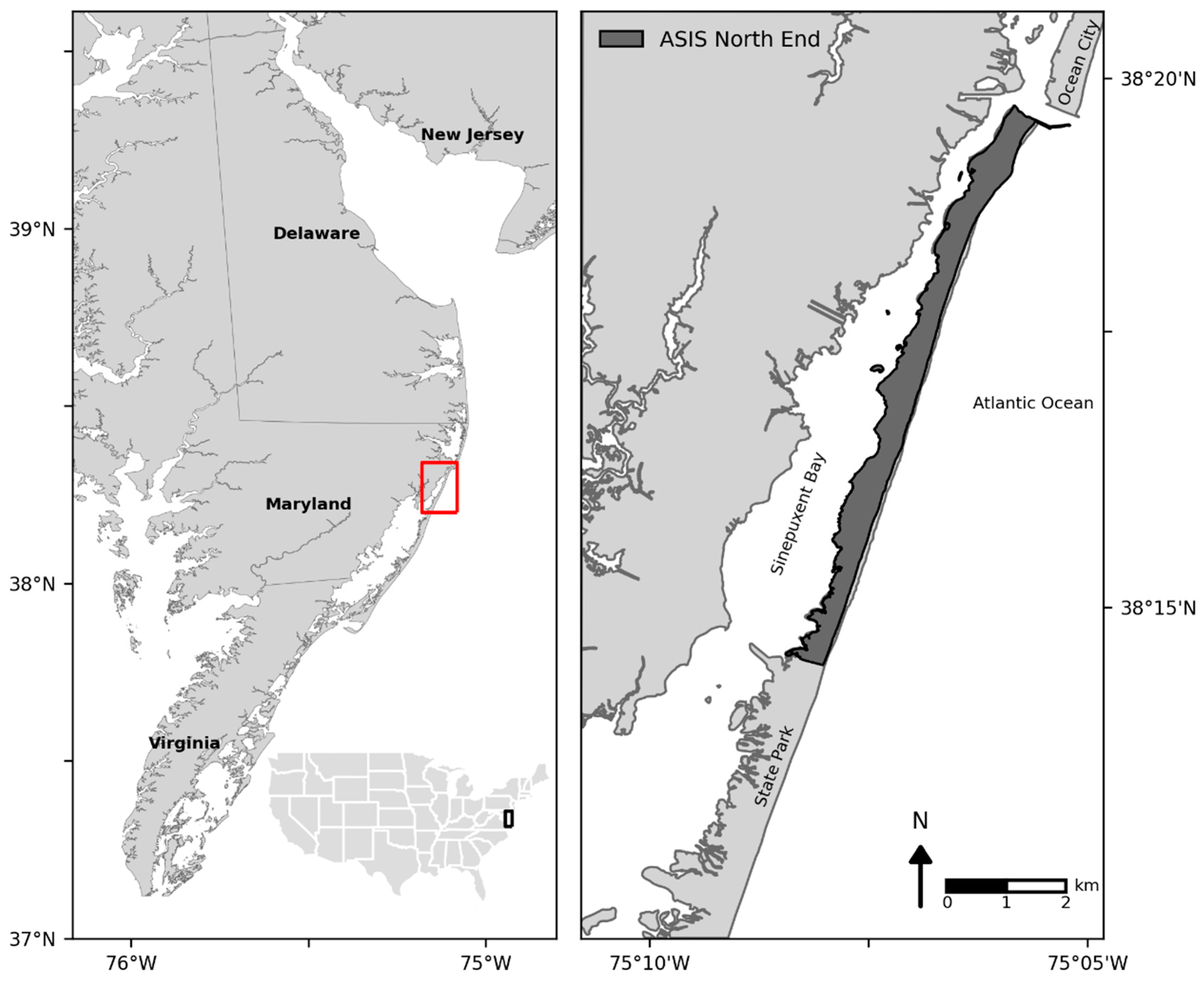
2. Study Area
3. Materials and Methods
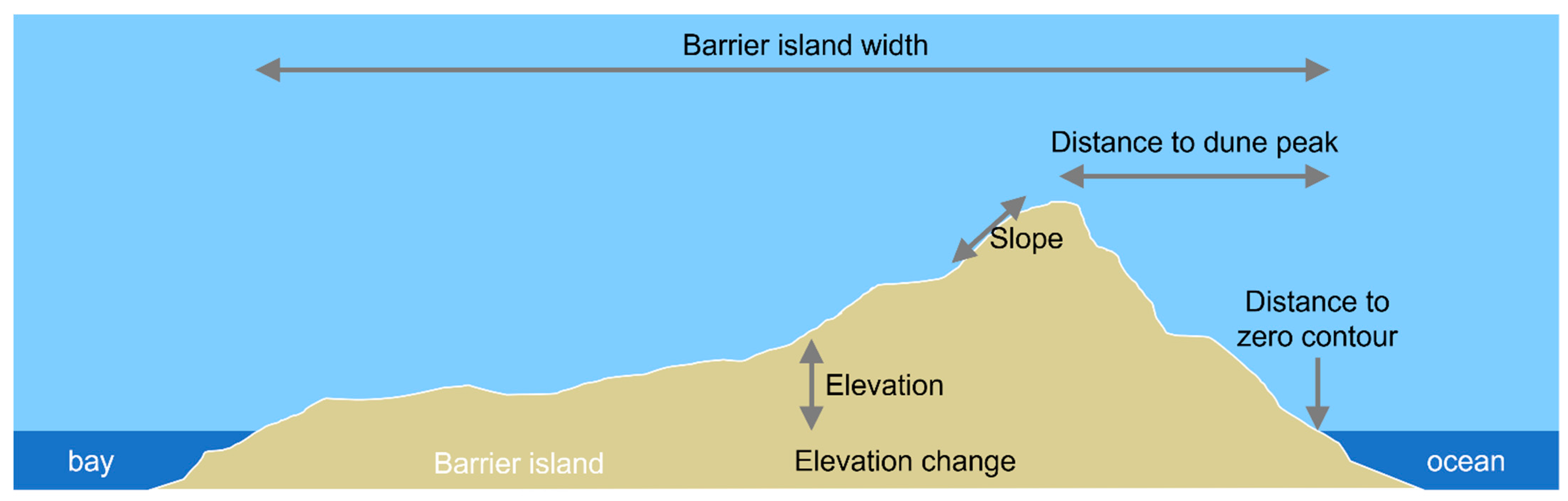
3.1. Geospatial Data and Processing
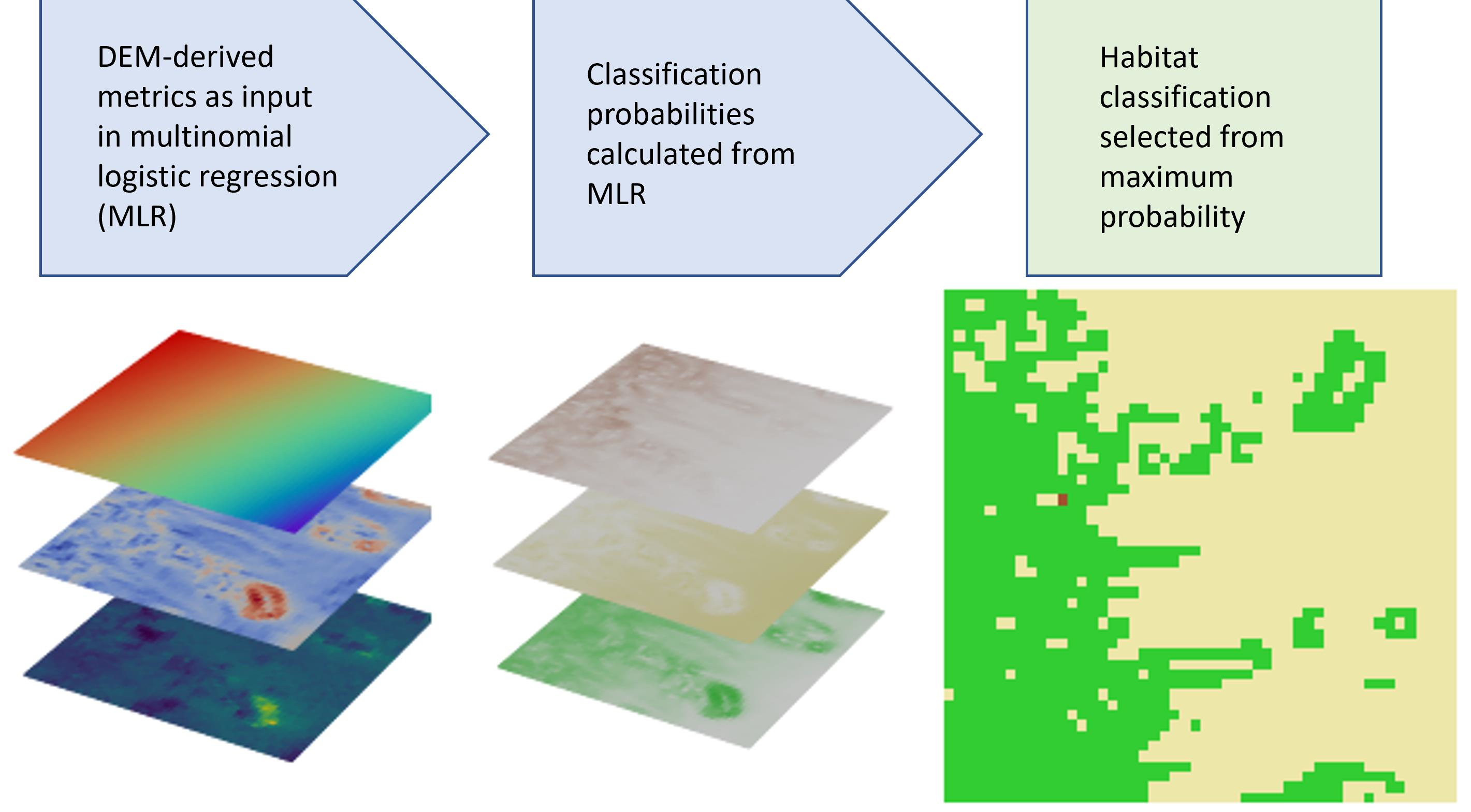
3.2. Model Development
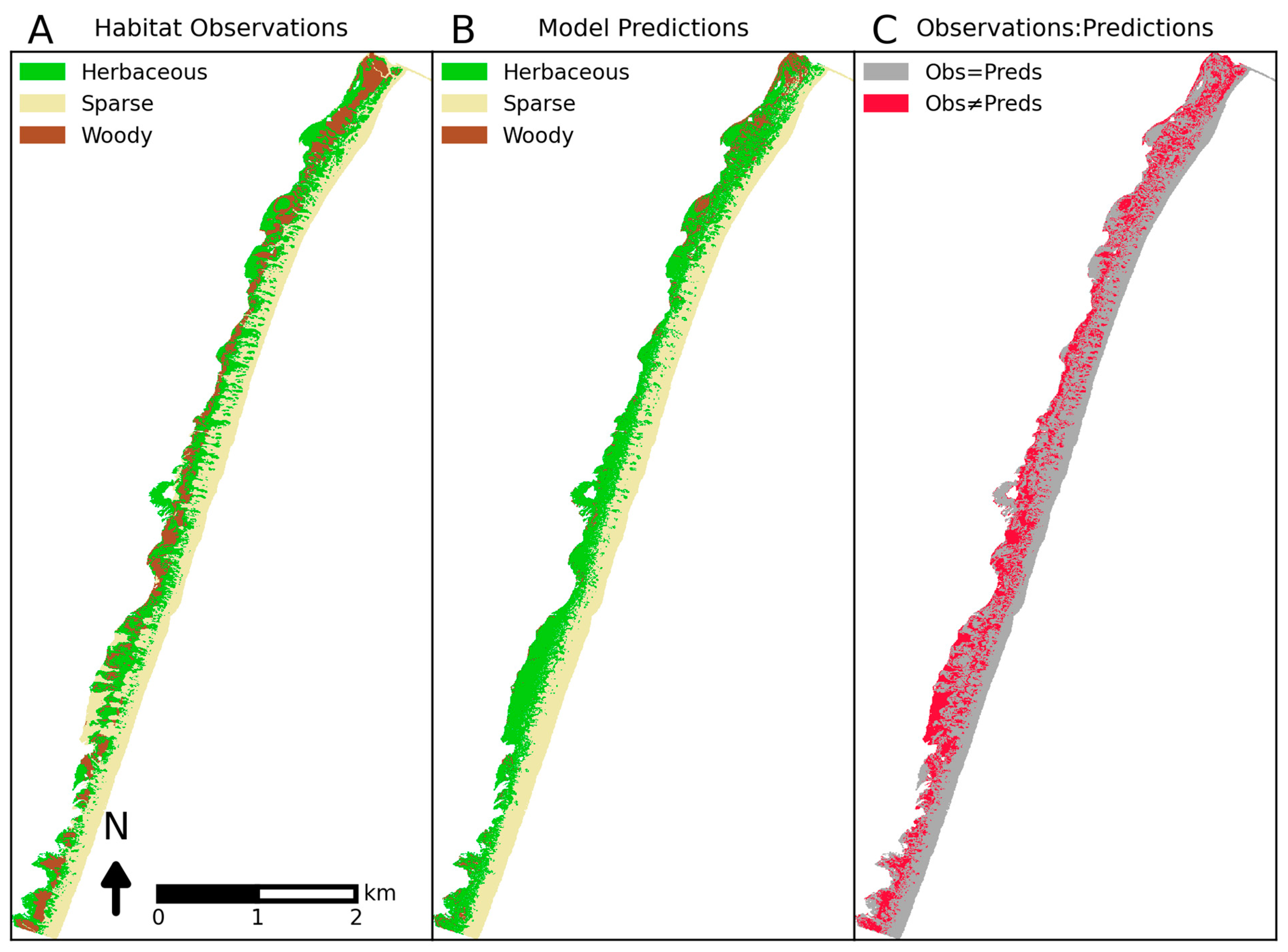
4. Results
5. Discussion
6. Conclusions
Supplementary Materials
Author Contributions
Funding
Institutional Review Board Statement
Informed Consent Statement
Data Availability Statement
Conflicts of Interest
References
- Luisetti, T.; Turner, R.K.; Jickells, T.; Andrews, J.; Elliott, M.; Schaafsma, M.; Beaumont, N.; Malcolm, S.; Burdon, D.; Adams, C.; et al. Coastal Zone Ecosystem Services: From science to values and decision making; a case study. Sci. Total Environ. 2014, 493, 682–693. [Google Scholar] [CrossRef] [PubMed]
- Arkema, K.K.; Guannel, G.; Verutes, G.; Wood, S.A.; Guerry, A.; Ruckelshaus, M.; Kareiva, P.; Lacayo, M.; Silver, J.M. Coastal habitats shield people and property from sea-level rise and storms. Nat. Clim. Chang. 2013, 3, 913–918. [Google Scholar] [CrossRef]
- IPCC. Climate Change 2014: Synthesis Report. Contribution of Working Groups I, II and III to the Fifth Assessment Report of the Intergovernmental Panel on Climate Change; Core Writing Team, Pachauri, R.K., Meyer, L.A., Eds.; IPCC: Geneva, Switzerland, 2014; p. 151. [Google Scholar]
- Altman, S.; Reif, M.K.; Swannack, T.M. Linking Critical Ecological Processes to Landscape Pattern: Implications for USACE Planning and Operations; ERDC/CHL CHETN-V-23; US Army Engineer Research and Development Center: Vicksburg, MS, USA, 2014; p. 9. [Google Scholar]
- Reif, M.K.; Swannack, T.M. Development of Landscape Metrics to Support Process-Driven Ecological Modeling; ERDC/EL TR-14-6; US Army Engineer Research and Development Center: Vicksburg, MS, USA, 2014; p. 38. [Google Scholar]
- Spalding, M.D.; Ruffo, S.; Lacambra, C.; Meliane, I.; Hale, L.Z.; Shepard, C.C.; Beck, M.W. The role of ecosystems in coastal protection: Adapting to climate change and coastal hazards. Ocean Coast. Manag. 2014, 90, 50–57. [Google Scholar] [CrossRef]
- Stallins, J.A.; Parker, A.J. The Influence of Complex Systems Interactions on Barrier Island Dune Vegetation Pattern and Process. Ann. Assoc. Am. Geogr. 2003, 93, 13–29. [Google Scholar] [CrossRef]
- Feagin, R.A.; Figlus, J.; Zinnert, J.C.; Sigren, J.; Martínez, M.L.; Silva, R.; Smith, W.K.; Cox, D.; Young, D.R.; Carter, G. Going with the flow or against the grain? The promise of vegetation for protecting beaches, dunes, and barrier islands from erosion. Front. Ecol. Environ. 2015, 13, 203–210. [Google Scholar] [CrossRef]
- Guisan, A.; Thuiller, W. Predicting species distribution: Offering more than simple habitat models. Ecol. Lett. 2005, 8, 993–1009. [Google Scholar] [CrossRef] [PubMed]
- Wiersma, Y.F.; Huettmann, F.; Drew, C.A. Introduction: Landscape modeling of species and their habitats: History, uncertainty, and complexity. In Predictive Species and Habitat Modeling in Landscape Ecology: Concepts and Applications; Springer: New York, NY, USA, 2011; pp. 1–6. ISBN 9781441973894. [Google Scholar]
- Hladik, C.; Alber, M. Classification of salt marsh vegetation using edaphic and remote sensing-derived variables. Estuar. Coast. Shelf Sci. 2014, 141, 47–57. [Google Scholar] [CrossRef]
- Dunkin, L.; Reif, M.; Altman, S.; Swannack, T. A Spatially Explicit, Multi-Criteria Decision Support Model for Loggerhead Sea Turtle Nesting Habitat Suitability: A Remote Sensing-Based Approach. Remote Sens. 2016, 8, 573. [Google Scholar] [CrossRef]
- Hood, W.G. Landscape allometry and prediction in estuarine ecology: Linking landform scaling to ecological patterns and processes. Estuaries Coasts 2007, 30, 895–900. [Google Scholar] [CrossRef]
- Hacker, S.D.; Jay, K.R.; Cohn, N.; Goldstein, E.B.; Hovenga, P.A.; Itzkin, M.; Moore, L.J.; Mostow, R.S.; Mullins, E.V.; Ruggiero, P. Species-specific functional morphology of four US atlantic coast dune grasses: Biogeographic implications for dune shape and coastal protection. Diversity 2019, 11, 82. [Google Scholar] [CrossRef]
- Charbonneau, B.R.; Dohner, S.M.; Wnek, J.P.; Barber, D.; Zarnetske, P.; Casper, B.B. Vegetation effects on coastal foredune initiation: Wind tunnel experiments and field validation for three dune-building plants. Geomorphology 2021, 378, 107594. [Google Scholar] [CrossRef]
- Miller, D.L.; Thetford, M.; Schneider, M. Distance from the Gulf Influences Survival and Growth of Three Barrier Island Dune Plants. J. Coast. Res. 2008, 4, 261–266. [Google Scholar] [CrossRef]
- Shao, G.; Shugart, H.H.; Hayden, B.P. Functional classifications of coastal barrier island vegetation. J. Veg. Sci. 1996, 7, 391–396. [Google Scholar] [CrossRef]
- Young, D.R.; Brantley, S.T.; Zinnert, J.C.; Vick, J.K. Landscape position and habitat polygons in a dynamic coastal environment. Ecosphere 2011, 2, art71. [Google Scholar] [CrossRef]
- Wernette, P.; Houser, C.; Bishop, M.P. An automated approach for extracting Barrier Island morphology from digital elevation models. Geomorphology 2016, 262, 1–7. [Google Scholar] [CrossRef]
- Enwright, N.M.; Wang, L.; Wang, H.; Osland, M.J.; Feher, L.C.; Borchert, S.M.; Day, R.H. Modeling Barrier Island Habitats Using Landscape Position Information. Remote Sens. 2019, 11, 976. [Google Scholar] [CrossRef]
- Brock, J.C.; Purkis, S.J. The emerging role of lidar remote sensing in coastal research and resource management. J. Coast. Res. 2009, 25, 1–5. [Google Scholar] [CrossRef]
- Gesch, D.B. Analysis of lidar elevation data for improved identification and delineation of lands vulnerable to sea-level rise. J. Coast. Res. 2009, 25, 49–58. [Google Scholar] [CrossRef]
- Stockdon, H.F.; Sallenger, A.H.; Holman, R.A.; Howd, P.A. A simple model for the spatially-variable coastal response to hurricanes. Mar. Geol. 2007, 238, 1–20. [Google Scholar] [CrossRef]
- Lopes, C.L.; Mendes, R.; Caçador, I.; Dias, J.M. Assessing salt marsh loss and degradation by combining long-term LANDSAT imagery and numerical modelling. L. Degrad. Dev. 2021, 32, 4534–4545. [Google Scholar] [CrossRef]
- McCarthy, M.J.; Halls, J.N. Habitat mapping and change assessment of coastal environments: An examination of worldview-2, quickbird, and ikonos satellite imagery and airborne lidar for mapping barrier island habitats. ISPRS Int. J. Geo-Inf. 2014, 3, 297–325. [Google Scholar] [CrossRef]
- Valentini, E.; Taramelli, A.; Cappucci, S.; Filipponi, F.; Xuan, A.N. Exploring the dunes: The correlations between vegetation cover pattern and morphology for sediment retention assessment using airborne multisensor acquisition. Remote Sens. 2020, 12, 1229. [Google Scholar] [CrossRef]
- Malthus, T.J.; Mumby, P.J. Remote sensing of the coastal zone: An overview and priorities for future research. Int. J. Remote Sens. 2003, 24, 2805–2815. [Google Scholar] [CrossRef]
- Sneddon, L.; Menke, J.; Berdine, A.; Largay, E.; Gawler, S. Vegetation classification and mapping of Assateague Island National Seashore. In Natural Resource Report NPS/ASIS/NRR—2017/1422; National Park Service: Fort Collins, CO, USA, 2017; pp. 1–119. [Google Scholar]
- Rossi, A.M.; Rabenhorst, M.C. Organic carbon dynamics in soils of Mid-Atlantic barrier island landscapes. Geoderma 2019, 337, 1278–1290. [Google Scholar] [CrossRef]
- Schupp, C.A.; Winn, N.T.; Pearl, T.L.; Kumer, J.P.; Carruthers, T.J.B.; Zimmerman, C.S. Restoration of overwash processes creates piping plover (Charadrius melodus) habitat on a barrier island (Assateague Island, Maryland). Estuar. Coast. Shelf Sci. 2013, 116, 11–20. [Google Scholar] [CrossRef]
- U.S. Army Corps of Engineers. Ocean City, Maryland and Vicinity Water Resources Study: Final Integrated Feasibility Report and Environmental Impact Statement; U.S. Army Corps of Engineers: Baltimore, MD, USA, 1998. [Google Scholar]
- Schupp, C.A.; Bass, G.P.; Grosskopf, W.G. Sand bypassing restores natural processes to Assateague Island, Maryland. In Proceedings of the Sixth International Symposium on Coastal Engineering and Science of Coastal Sediment Process, New Orleans, Louisiana, 13–17 May 2007. [Google Scholar] [CrossRef]
- Carruthers, T.J.B.; Beckert, K.; Schupp, C.A.; Saxby, T.; Kumer, J.P.; Thomas, J.; Sturgis, B.; Dennison, W.C.; Williams, M.; Fisher, T.; et al. Improving management of a mid-Atlantic coastal barrier island through assessment of habitat condition. Estuar. Coast. Shelf Sci. 2013, 116, 74–86. [Google Scholar] [CrossRef]
- Roman, C.T.; Nordstrom, K.F. The effect of erosion rate on vegetation patterns of an east coast barrier island. Estuar. Coast. Shelf Sci. 1988, 26, 233–242. [Google Scholar] [CrossRef]
- OCM: Office for Coastal Management. 2000 Fall East Coast NOAA/USGS/NASA Airborne LiDAR Assessment of Coastal Erosion (ALACE) Project for the US Coastline. Available online: https://www.fisheries.noaa.gov/inport/item/48163 (accessed on 1 June 2021).
- OCM. USACE Post Sandy Topographic LiDAR: Virginia and Maryland. 2012. Available online: https://www.fisheries.noaa.gov/inport/item/49610 (accessed on 1 June 2021).
- Pedregosa, F.; Varoquaux, G.; Gramfort, A.; Michel, V.; Thirion, B.; Grisel, O.; Blondel, M.; Prettenhofer, P.; Weiss, R.; Dubourg, V. Scikit-learn: Machine learning in Python. J. Mach. Learn. Res. 2011, 12, 2825–2830. [Google Scholar]
- Cohen, J. A Coefficient of Agreement for Nominal Scales. Educ. Psychol. Meas. 1960, 20, 37–46. [Google Scholar] [CrossRef]
- Allouche, O.; Tsoar, A.; Kadmon, R. Assessing the accuracy of species distribution models: Prevalence, kappa and the true skill statistic (TSS). J. Appl. Ecol. 2006, 43, 1223–1232. [Google Scholar] [CrossRef]
- Rossi, A.M. Pedogenesis and Hydrogeomorphology of Soils in Mid-Atlantic Barrier Island Landscapes. Doctoral Dissertation, University of Maryland, College Park, MD, USA, 2014. [Google Scholar]
- Landis, J.R.; Koch, G.G. The Measurement of Observer Agreement for Categorical Data. Biometrics 1977, 33, 159. [Google Scholar] [CrossRef] [PubMed]
- Zinnert, J.C.; Stallins, J.A.; Brantley, S.T.; Young, D.R. Crossing scales: The complexity of barrier-island processes for predicting future change. Bioscience 2017, 67, 39–52. [Google Scholar] [CrossRef]
- Brantley, S.T.; Bissett, S.N.; Young, D.R.; Wolner, C.W.V.; Moore, L.J. Barrier island morphology and sediment characteristics affect the recovery of dune building grasses following storm-induced overwash. PLoS ONE 2014, 9, e104747. [Google Scholar] [CrossRef] [PubMed]
- Nardin, W.; Larsen, L.; Fagherazzi, S.; Wiberg, P. Tradeoffs among hydrodynamics, sediment fluxes and vegetation community in the Virginia Coast Reserve, USA. Estuar. Coast. Shelf Sci. 2018, 210, 98–108. [Google Scholar] [CrossRef]
- Zinnert, J.C.; Shiflett, S.A.; Via, S.; Bissett, S.; Dows, B.; Manley, P.; Young, D.R. Spatial–Temporal Dynamics in Barrier Island Upland Vegetation: The Overlooked Coastal Landscape. Ecosystems 2016, 19, 685–697. [Google Scholar] [CrossRef]
- Zeigler, S.L.; Sturdivant, E.J.; Gutierrez, B.T. Evaluating Barrier Island Characteristics and Piping Plover (Charadrius Melodus) Habitat Availability along the U.S. Atlantic Coast—Geospatial Approaches and Methodology; Open-File Report 2019–1071; U.S. Geological Survey: Reston, VA, USA, 2019; p. 34. [Google Scholar]
- Houser, C.; Hapke, C.; Hamilton, S. Controls on coastal dune morphology, shoreline erosion and barrier island response to extreme storms. Geomorphology 2008, 100, 223–240. [Google Scholar] [CrossRef]
- Small-Lorenz, S.L.; Shadel, W.P.; Glick, P. Building Ecological Solutions to Coastal Community Hazards; The National Wildlife Federation: Washington, DC, USA, 2017; p. 95. [Google Scholar]
- Halls, J.N.; Frishman, M.A.; Hawkes, A.D. An automated model to classify barrier island geomorphology using lidar data and change analysis (1998–2014). Remote Sens. 2018, 10, 1109. [Google Scholar] [CrossRef]
- Hayden, B.P.; Santos, M.C.F.V.; Shao, G.; Kochel, R.C. Geomorphological controls on coastal vegetation at the Virginia Coast Reserve. Geomorphology 1995, 13, 283–300. [Google Scholar] [CrossRef]
- Young, D.R.; Porter, J.H.; Bachmann, C.M.; Shao, G.; Fusina, R.A.; Bowles, J.H.; Korwan, D.; Donato, T.F. Cross-scale patterns in shrub thicket dynamics in the Virginia barrier complex. Ecosystems 2007, 10, 854–863. [Google Scholar] [CrossRef]
- Young, D.R.; Shao, G.; Porter, J.H. Spatial and temporal growth dynamics of barrier island shrub thickets. Am. J. Bot. 1995, 82, 638–645. [Google Scholar] [CrossRef]
- Doyle, T.B.; Woodroffe, C.D. The application of LiDAR to investigate foredune morphology and vegetation. Geomorphology 2018, 303, 106–121. [Google Scholar] [CrossRef]
- Ray, N.; Burgman, M.A. Subjective uncertainties in habitat suitability maps. Ecol. Modell. 2006, 195, 172–186. [Google Scholar] [CrossRef]
- Enwright, N.M.; Wang, L.; Borchert, S.M.; Day, R.H.; Feher, L.C.; Osland, M.J. Advancing barrier island habitat mapping using landscape position information. Prog. Phys. Geogr. Earth Environ. 2019, 43, 425–450. [Google Scholar] [CrossRef]
- Houser, C.; Bishop, M.; Wernette, P. Short communication: Multi-scale topographic anisotropy patterns on a Barrier Island. Geomorphology 2017, 297, 153–158. [Google Scholar] [CrossRef]
- Feilhauer, H.; Thonfeld, F.; Faude, U.; He, K.S.; Rocchini, D.; Schmidtlein, S. Assessing floristic composition with multispectral sensors-A comparison based: On monotemporal and multiseasonal field spectra. Int. J. Appl. Earth Obs. Geoinf. 2012, 21, 218–229. [Google Scholar] [CrossRef]
- García-Romero, L.; Hernández-Cordero, A.I.; Hernández-Calvento, L.; Espino, E.P.-C.; López-Valcarcel, B.G. Procedure to automate the classification and mapping of the vegetation density in arid aeolian sedimentary systems. Prog. Phys. Geogr. Earth Environ. 2018, 42, 330–351. [Google Scholar] [CrossRef]
- Aguilar, C.; Zinnert, J.C.; Polo, M.J.; Young, D.R. NDVI as an indicator for changes in water availability to woody vegetation. Ecol. Indic. 2012, 23, 290–300. [Google Scholar] [CrossRef]
- Klemas, V. Beach profiling and LIDAR bathymetry: An overview with case studies. J. Coast. Res. 2011, 27, 1019–1028. [Google Scholar] [CrossRef]
- Chan, K.M.A.; Pringle, R.M.; Ranganathan, J.; Boggs, C.L.; Chan, Y.L.; Ehrlich, P.R.; Haff, P.K.; Heller, N.E.; Al-Khafaji, K.; Macmynowski, D.P. When Agendas Collide: Human Welfare and Biological Conservation. Conserv. Biol. 2007, 21, 59–68. [Google Scholar] [CrossRef] [PubMed]
- Brantley, S.T.; Young, D.R. Shifts in litterfall and dominant nitrogen sources after expansion of shrub thickets. Oecologia 2008, 155, 337–345. [Google Scholar] [CrossRef] [PubMed]
- Brantley, S.T.; Young, D.R. Shrub expansion stimulates soil C and N storage along a coastal soil chronosequence. Glob. Chang. Biol. 2010, 16, 2052–2061. [Google Scholar] [CrossRef]
- Huang, H.; Zinnert, J.C.; Wood, L.K.; Young, D.R.; D’Odorico, P. Non-linear shift from grassland to shrubland in temperate barrier islands. Ecology 2018, 99, 1671–1681. [Google Scholar] [CrossRef] [PubMed]
- Theuerkauf, E.J.; Rodriguez, A.B. Placing barrier-island transgression in a blue-carbon context. Earth’s Futur. 2017, 5, 789–810. [Google Scholar] [CrossRef]
- Duarte, C.M.; Dennison, W.C.; Orth, R.J.W.; Carruthers, T.J.B. The Charisma of Coastal Ecosystems: Addressing the Imbalance. Estuaries Coasts 2008, 31, 233–238. [Google Scholar] [CrossRef]
- Duarte, C.M.; Losada, I.J.; Hendriks, I.E.; Mazarrasa, I.; Marbà, N. The role of coastal plant communities for climate change mitigation and adaptation. Nat. Clim. Chang. 2013, 3, 961–968. [Google Scholar] [CrossRef]
- Beaumont, N.J.; Jones, L.; Garbutt, A.; Hansom, J.D.; Toberman, M. The value of carbon sequestration and storage in coastal habitats. Estuar. Coast. Shelf Sci. 2014, 137, 32–40. [Google Scholar] [CrossRef]
- Drius, M.; Carranza, M.L.; Stanisci, A.; Jones, L. The role of Italian coastal dunes as carbon sinks and diversity sources. A multi-service perspective. Appl. Geogr. 2016, 75, 127–136. [Google Scholar] [CrossRef]


| Year | Cell Size (m) | Vertical Accuracy (cm) | Horizontal Accuracy (cm) | Agency | Sensor |
|---|---|---|---|---|---|
| 2000 | 3 | 15 | 80 | NOAA, NASA, USGS | Airborne Topographic Mapper |
| 2012 * | 1 | 7 | 30 | USACE | Optech Gemini Lidar Sensor |
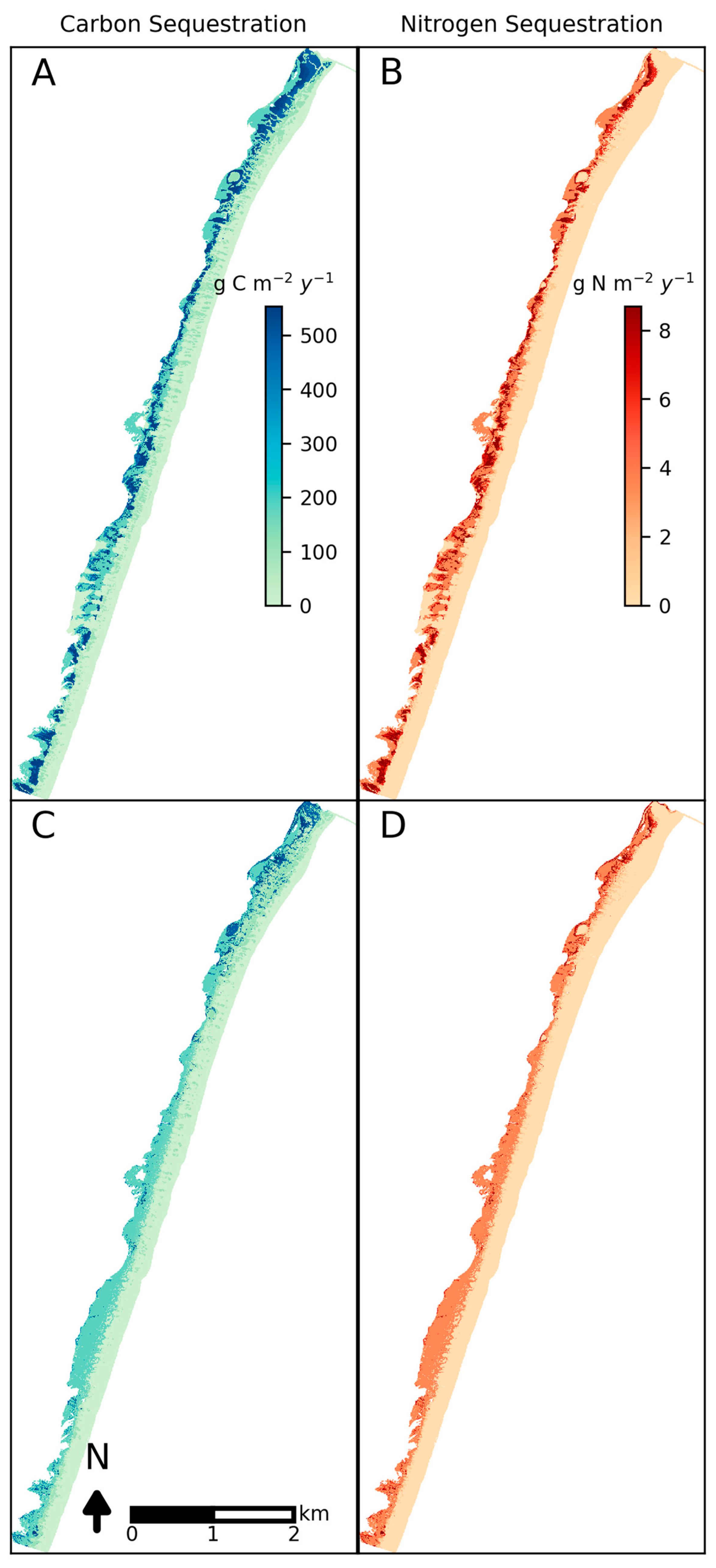
| Habitat | Elevation Range (m) | Carbon Sequestration (g C m−2 y−1) | Nitrogen Sequestration (g N m−2 y−1) |
|---|---|---|---|
| Herbaceous | 0.00–0.66 | 181.04 ± 15.74 | 3.52 ± 0.33 |
| 0.67–1.04 | 171.25 ± 30.67 | 3.68 ± 0.72 | |
| 1.05–1.41 | 65.28 ± 11.97 | 1.36 ± 0.27 | |
| >1.41 | 112.00 ± 14.00 | 2.24 ± 0.28 | |
| Woody | −0.02–0.38 | 447.29 ± 56.09 | 6.65 ± 0.93 |
| 0.39–0.79 | 553.90 ± 87.97 | 8.70 ± 1.59 | |
| 0.80–1.20 | 531.97 ± 41.88 | 6.14 ± 0.76 | |
| >1.20 | 497.00 ± 43.00 | 5.58 ± 0.48 |
| Parameter | Minimum | Maximum | Mean | Std. Dev |
|---|---|---|---|---|
| All (n = 161,346) | ||||
| Elevation difference (m) | −5.89 | 3.09 | 0.15 | 0.53 |
| [Slope (%)]1/3 | 0.00 | 2.81 | 0.98 | 0.33 |
| [Distance to shore (m)]1/3 | 0.00 | 8.68 | 5.84 | 1.37 |
| [Slope*Distance to shore]1/3 | 0.00 | 21.14 | 5.62 | 2.08 |
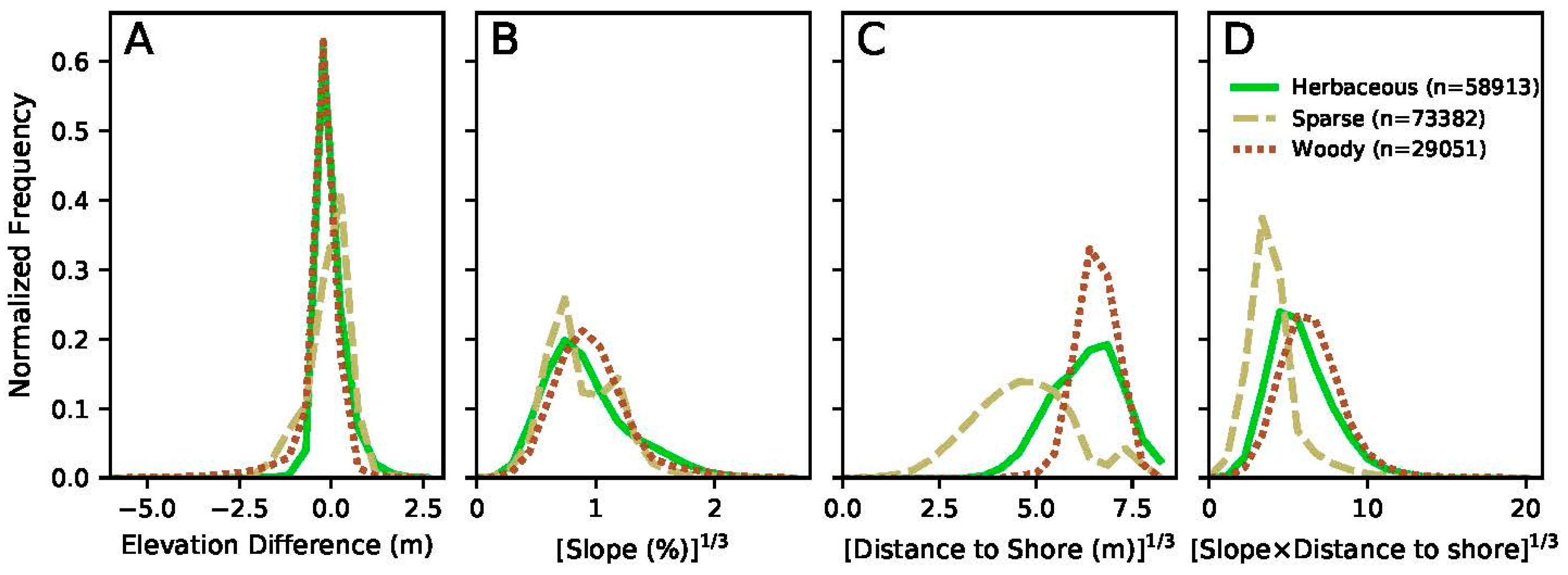
| Herbaceous (n = 58,913) | ||||
| Elevation difference (m) | −2.66 | 3.09 | 0.23 | 0.39 |
| [Slope (%)]1/3 | 0.00 | 2.64 | 0.99 | 0.36 |
| [Distance to shore (m)]1/3 | 3.56 | 8.68 | 6.54 | 0.91 |
| [Slope*Distance to shore]1/3 | 0.00 | 18.85 | 6.33 | 1.98 |
| Sparse (n = 73,382) | ||||
| Elevation difference (m) | −4.22 | 2.90 | 0.17 | 0.57 |
| [Slope (%)]1/3 | 0.00 | 2.68 | 0.95 | 0.30 |
| [Distance to shore (m)]1/3 | 0.00 | 8.60 | 4.91 | 1.31 |
| [Slope*Distance to shore]1/3 | 0.0 | 19.93 | 4.50 | 1.55 |
| Woody (n = 29,051) | ||||
| Elevation difference (m) | −5.89 | 2.83 | −0.04 | 0.60 |
| [Slope (%)]1/3 | 0.00 | 2.81 | 1.04 | 0.31 |
| [Distance to shore (m)]1/3 | 4.57 | 8.16 | 6.79 | 1.31 |
| [Slope*Distance to shore]1/3 | 0.00 | 21.14 | 6.99 | 2.00 |
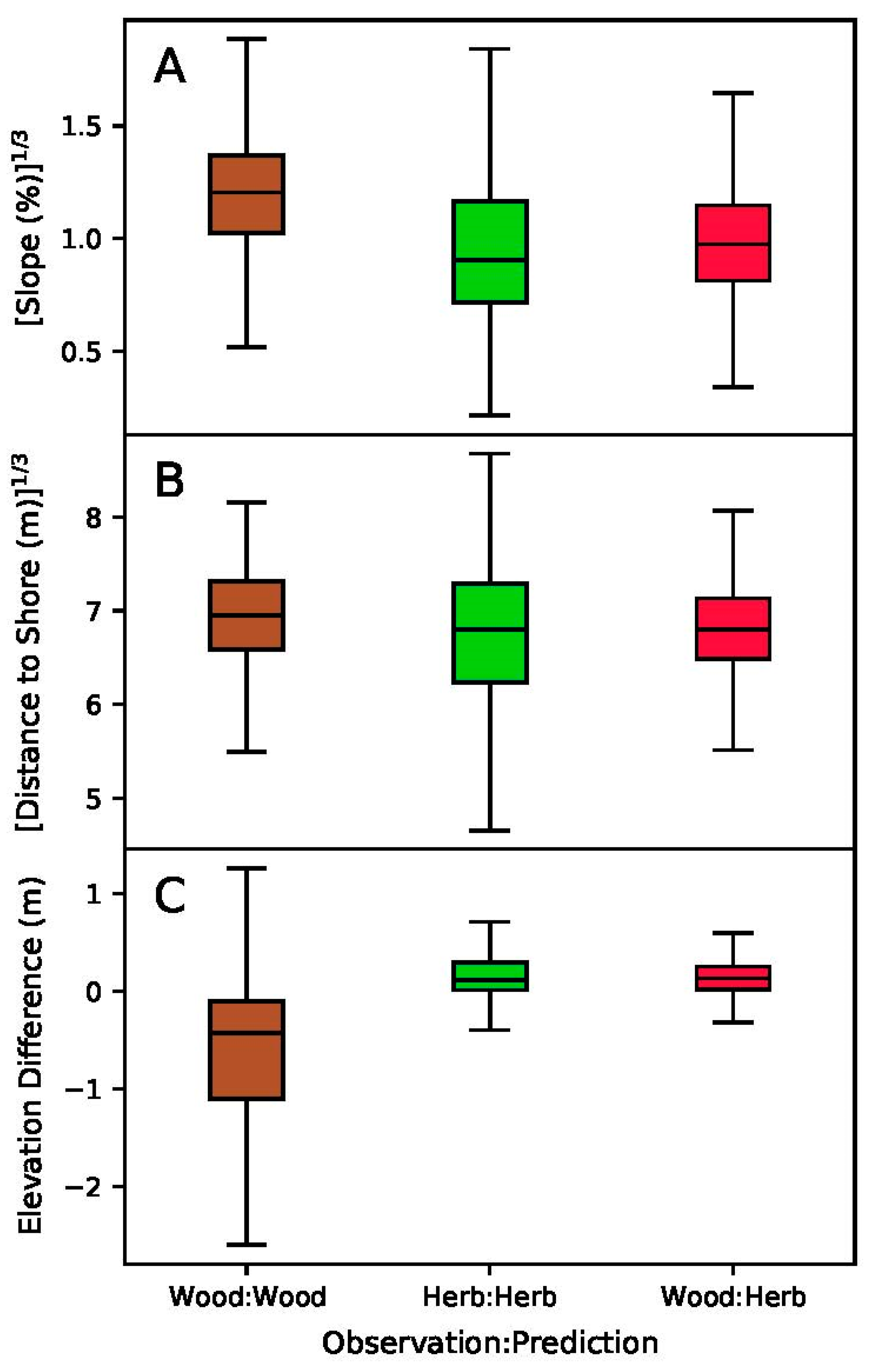
| Intercept | Elevation Difference | Slope(1/3) | Distance to Shore(1/3) | (Slope × Distance to Shore)(1/3) | |
|---|---|---|---|---|---|
| Herbaceous | −6.56 | −0.63 | 3.87 | 0.98 | −0.50 |
| Sparse | 7.82 | 0.08 | −0.03 | −0.94 | −0.32 |
| Woody | −1.26 | −0.71 | −3.84 | −0.03 | 0.82 |
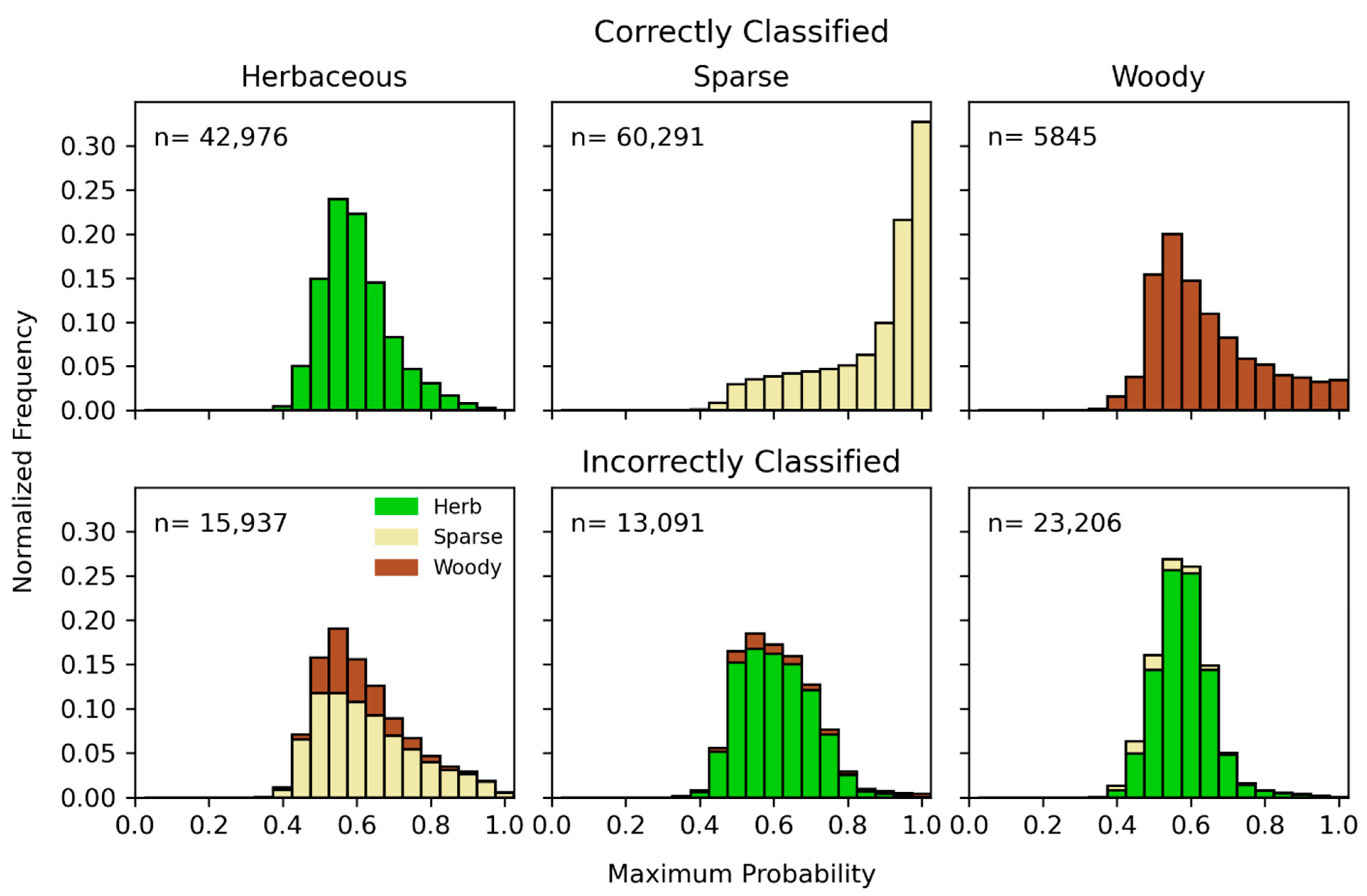
| Predictions | |||||
|---|---|---|---|---|---|
| Habitat | Herbaceous | Sparse | Woody | Total | |
| Observations | Herbaceous | 42,976 | 11,944 | 3993 | 58,913 |
| Sparse | 12,000 | 60,291 | 1091 | 73,382 | |
| Woody | 21,656 | 1550 | 5845 | 29,051 | |
| Total | 76,632 | 73,785 | 10,929 | 161,346 | |
Publisher’s Note: MDPI stays neutral with regard to jurisdictional claims in published maps and institutional affiliations. |
© 2022 by the authors. Licensee MDPI, Basel, Switzerland. This article is an open access article distributed under the terms and conditions of the Creative Commons Attribution (CC BY) license (https://creativecommons.org/licenses/by/4.0/).
Share and Cite
Russ, E.R.; Charbonneau, B.R.; Altman, S.; Reif, M.K.; Swannack, T.M. Habitat Classification Predictions on an Undeveloped Barrier Island Using a GIS-Based Landscape Modeling Approach. Remote Sens. 2022, 14, 1377. https://doi.org/10.3390/rs14061377
Russ ER, Charbonneau BR, Altman S, Reif MK, Swannack TM. Habitat Classification Predictions on an Undeveloped Barrier Island Using a GIS-Based Landscape Modeling Approach. Remote Sensing. 2022; 14(6):1377. https://doi.org/10.3390/rs14061377
Chicago/Turabian StyleRuss, Emily R., Bianca R. Charbonneau, Safra Altman, Molly K. Reif, and Todd M. Swannack. 2022. "Habitat Classification Predictions on an Undeveloped Barrier Island Using a GIS-Based Landscape Modeling Approach" Remote Sensing 14, no. 6: 1377. https://doi.org/10.3390/rs14061377
APA StyleRuss, E. R., Charbonneau, B. R., Altman, S., Reif, M. K., & Swannack, T. M. (2022). Habitat Classification Predictions on an Undeveloped Barrier Island Using a GIS-Based Landscape Modeling Approach. Remote Sensing, 14(6), 1377. https://doi.org/10.3390/rs14061377