IMU-Aided Registration of MLS Point Clouds Using Inertial Trajectory Error Model and Least Squares Optimization

Abstract

Mobile laser scanning (MLS) point cloud registration plays a critical role in mobile 3D mapping and inspection, but conventional point cloud registration methods for terrain LiDAR scanning (TLS) are not suitable for MLS. To cope with this challenge, we use inertial measurement unit (IMU) to assist registration and propose an MLS point cloud registration method based on an inertial trajectory error model. First, we propose an error model of inertial trajectory over a short time period to construct the constraints between trajectory points at different times. On this basis, a relationship between the point cloud registration error and the inertial trajectory error is established, then trajectory error parameters are estimated by minimizing the point cloud registration error using the least squares optimization. Finally, a reliable and concise inertial-assisted MLS registration algorithm is realized. We carried out experiments in three different scenarios: indoor, outdoor and integrated indoor–outdoor. We evaluated the overall performance, accuracy and efficiency of the proposed method. Compared with the ICP method, the accuracy and speed of the proposed method were improved by 2 and 2.8 times, respectively, which verified the effectiveness and reliability of the proposed method. Furthermore, experimental results show the significance of our method in constructing a reliable and scalable mobile 3D mapping system suitable for complex scenes.

1. Introduction

Large-scene 3D point cloud data acquisition is one of the foundations of 3D mapping and inspection [1], and mobile LiDAR scanning (MLS) technology provides an accurate and efficient way to obtain large-scene 3D point cloud data [2]. MLS technology uses LiDAR installed on a mobile platform to scan the environment. Due to the limited scanning range of a single LiDAR frame, it is necessary to convert the scan frames at different positions into a unified coordinate system to merge a large-scene 3D point cloud. This registration process plays a critical role in MLS data processing [3]. Traditional MLS technology uses a GNSS/INS system to obtain the pose of the carrier. Position and attitude in the unified mapping frame are given to each laser point according to the sampling time to realize the registration of MLS point clouds. When GNSS is denied or disturbed, the GNSS/INS trajectory error will rapidly increase, leading to an increase in the registration error and resulting in ghosting or deformation. With the increasing demand for 3D mapping and inspection in complex scenes, such as indoor and underground spaces, the development of MLS registration methods independent of GNSS systems has become a research hotspot [4].

A conventional point cloud registration method generally needs to first identify the correspondences between scan frames and then estimate their transformation model [5]. These “LiDAR-only” methods focus on the characteristics of point cloud data without the assistance of auxiliary information. They are generally designed for point clouds using fixed-station LiDAR, and the motions between different stations are rigid transformation models [6,7,8]. However, for MLS data in complex environments, conventional point cloud registration methods are affected by unfavorable conditions, such as motion, homogeneous features and occlusion, making it difficult to achieve robust 3D reconstruction.

To improve the robustness and reliability of registration for the MLS point clouds in complex scenes, auxiliary sensors (such as IMUs, GNSS or cameras) are usually used to measure and compensate for irregular motion [9,10]. These methods [11,12,13,14,15] use visual features and GNSS absolute pose to assist point cloud registration, but they have limitations in complex environments, visual features are prone to degradation in weak texture environments, and GNSS fails in GNSS-denied environments. Unlike the above auxiliary sensors, IMU provides accurate pose over a short time and is environment-independent, so IMU and LiDAR have good complementarity [16]. However, existing studies [17,18] do not consider long-term IMU error drift, and they fail to construct rigorous optimization models using the correlation between IMU and point cloud data, so their robustness is poor in complex environments.

The fusion of LiDAR and IMUs has been extensively studied in the field of simultaneous localization and mapping (SLAM). LiDAR-inertial SLAM is dedicated to obtaining large-scene 3D maps and trajectories, so it also needs to solve the MLS registration problem. In these SLAM methods, IMU and LiDAR measurements are optimized in different ways to obtain high-precision motion estimation [19,20]. Compared with inertial-assisted registration methods [17,18], the SLAM-based methods adopt a complex optimization model and loop-detection process to optimize error. Although their accuracy is improved, the system is complex [21] and is difficult to extend, so it is not suitable for diversified task requirements in complex environments.

In short, a conventional static registration method [6] cannot guarantee robustness, due to fast motion, environmental occlusion and repetitive structures in complex environments. Existing multisensor fusion-based MLS registration methods [17,18] do not establish a rigorous optimization model for the correlation of multisource measurements, resulting in poor accuracy and reliability. SLAM methods are complex and difficult to extend, which is not conducive to practical application.

Aiming at the problem of MLS point cloud registration in complex environments, we propose an inertial-aided MLS point cloud registration method. We propose a new error model of inertial trajectory over a short time period to form constraints between LiDAR scan frames, then we optimize the inertial trajectory error and point cloud registration errors at the same time using least squares optimization. Finally, we achieve multi-frame MLS point cloud registration. The proposed method not only realizes high precision and reliability, but also constructs a concise LiDAR-inertial fusion model, which is easy to implement, apply and extend. Compared with conventional registration methods, our method shows accuracy improvement with the assistance of IMU; our method also outperforms existing IMU-aided registration methods, which benefit from the proposed error model. Furthermore, our proposed registration framework utilizes least squares to jointly optimize IMU and point cloud errors, thereby skipping the complex back-end optimization of SLAM, so it has better simplicity and extendibility than SLAM-based methods. Therefore, our method shows superiority in approaching the MLS registration problem.

The main contributions of this paper are as follows. (1) We propose a new inertial trajectory error model, which constructs constraints between LiDAR scan frames in a short-time window, and at the same time avoids the effect of long-term IMU drift on registration accuracy. (2) We propose a new inertial-aided MLS point cloud registration framework, which optimizes the inertial trajectory error model parameters and point cloud registration errors at the same time using least squares optimization, and achieves continuous LiDAR scan frame registration. The proposed registration framework has the characteristics of high precision, simplicity and extendibility. (3) A continuous cross-matching strategy is proposed to ensure high-overlap between LiDAR scan frames and effectively improve the reliability of registration.

The rest of this paper is arranged as follows. Section 2 introduces the related works. Section 3 introduces detailed technical route of this method, and Section 4 verifies the effectiveness of this method through experiments. Section 5 discusses the characteristics, applicable scenarios and limitations of this method. Finally, we summarize the content of this paper in Section 6.

2. Related Work

Identifying the correspondences is the key to conventional static point cloud registration, and methods for finding correspondences can be divided into two main categories: one type is based on the nearest neighbor relationship, such as ICP and its extended versions [6,22,23,24,25], which requires accurate initial estimation of the transformation. The other type is the feature-based matching method, whose performances are influenced by the geometric characteristics of point clouds, such as fast point feature histograms (FPFHs) [26], rotated projection statistics (RoPS) [27], signatures of histograms of orientations (SHOT) [28] and four-point congruent sets (4PCs) [7]. In addition to these two categories, deep learning methods have emerged in recent years, such as PointNet and its extended versions [8,29,30], which directly learn features using neural networks. For MLS data, conventional point cloud registration methods have the following problems. (1) Due to the movement of the carrier platform, the motion between LiDAR scan frames may not be a rigid transformation, which can greatly affect the precision of a registration method based on a rigid motion model. (2) When there is large angular motion, the difference between adjacent frames is large, so it is difficult to identify correspondences through a nearest neighbor search. As a result, ICP-based methods tend to fail without accurate initial values. (3) For scenes with repetitive or homogeneous structures (such as long corridors), mismatches will increase due to the ambiguity of features.

For multi-sensor-aided registration methods, the auxiliary sensors include camera, GNSS and IMU. Images usually contain a variety of visual information. The 2D features extracted from images can be mapped to 3D space to assist with point cloud feature extraction, which improves the reliability and robustness of feature-based point cloud registration [11,12,13]. However, visual features will be affected by lighting conditions and image textures, and may fail in complex environments. GNSS provides an absolute position and can also assist in eliminating registration error [14], but in urban and indoor environments, GNSS signals are denied [15]. An IMU provides accurate pose (especially rotation) over a short time and is environment independent, but drift will occur over long periods of time. LiDAR provides accurate and stable distance observations, but the MLS point cloud will be distorted because of the motion of the carrier. Therefore, IMU and LiDAR have good complementarity [16]. Some professional mobile mapping systems (MMSs) use IMUs to provide accurate initial estimations [9] for ICP. The studies [17] and [18] proposed trajectory-based MLS registration methods, which use a trajectory estimated using MMS to assist with point cloud registration. In [17], the researchers used MMS equipped with GNSS/INS to first estimate the initial trajectory, divided the trajectory into local areas for local point cloud registration, and then optimized the trajectory by performing least squares optimization. Finally, the overall point cloud was optimized globally based on the optimized trajectory. The study [18] extended [17] by introducing the minimum distance between a point and surface into the ICP algorithm and introducing rotation restriction to further improve registration accuracy. However, the studies in [17,18] only treated the trajectory as a prior estimation to assist registration. Since the influence of long-term IMU error drift and GNSS failure on MMS trajectory estimation was not considered and the correlation between IMU and point cloud data was not used to construct a rigorous optimization model, the robustness is poor in complex environments. Recently, the IMU pre-integration model proposed by [31,32] improved the accuracy and efficiency of IMU-LiDAR fusion. The study [33] adopted the time information provided by multi-sensors to assist the registration, which further improves the effect of point cloud registration, but [32,33] used tightly coupled optimization method, and inevitably needed much more space for online processing. Our proposed IMU error model is inspired by [31] and we adopt IMU pre-integration, but our optimization process is more concise and efficient.

In recent years, SLAM-based LiDAR-inertial fusion methods have been extensively studied. However, in this paper we only focused on the point cloud registration part of the front-end, and we did not describe the back-end optimization part in detail. Existing LiDAR-inertial odometers usually use IMU motion estimation as an initial value to assist LiDAR scan matching, such as the representative LOAM [34]. IN2LAMA [35] performs IMU pre-integration and up-sampling so that the time frequency of the up-sampled IMU measurements is the same as that of the LiDAR. Finally, the pre-integrated IMU value and LiDAR are fused for registration. The registration part of the loosely-coupled SLAM algorithm [34,35] only treats the IMU as auxiliary assistance, and the correlation between IMU error and point cloud registration error is not analyzed, resulting in poor robustness in complex environments. Tightly coupled methods [36,37,38] consider the correlation between the IMU and point cloud measurements, and usually add a step to optimize IMU estimation, using feedback from point cloud registration results. LVIO [39] estimates motion through visual-inertial odometry, then carries out LiDAR scan matching with the assistance of visual-inertial estimation and feeds back the matching results for further iterative optimization. LVI-SAM [16] uses IMU estimation as an initial value for scan matching, and then the result of a LiDAR-inertial odometer is fed back to correct the IMU error, which improves the accuracy and robustness of point cloud registration. The registration part in the above SLAM methods usually uses IMU estimation as a prior to assist registration, then optimizes state estimations through an optimization framework, such as Kalman filtering or bundle adjustment, and uses loop detection to reduce accumulated errors. Compared with inertial-assisted registration methods [17,18], their fusion method between IMU and LiDAR is similar, but a complex optimization model and loop detection process are added to optimize error. Although the positioning accuracy is improved, the system is complex [21] and is difficult to extend, so it is not suitable for diversified task requirements in complex environments. Compared with these SLAM-based methods, we optimized IMU error and point cloud registration errors at the same time using least squares, and the proposed registration framework has the characteristics of high precision, simplicity and extendibility.

3. Methods

The research object of this paper is a measurement system composed of a multiline LiDAR and an IMU, in which the LiDAR and IMU are fixedly connected. The system can realize the synchronous measurement of the geometric features of environment (LiDAR) and the motion information (IMU) of the carrier (Figure 1).

Due to IMU device error and measurement noise, the trajectory error of IMU integration alone will diverge with time, so the trajectory of IMU integration cannot be directly used for the registration of sequence point clouds over a long time period (Figure 2). Therefore, we first analyze the error sources of IMU integration in detail and then construct an inertial trajectory error model, which can describe the error regularity of an IMU integration trajectory over a short time period and form a constraint between trajectory points at different times. Furthermore, we analyze the relationship between the point cloud registration error and inertial trajectory error and construct an inertial-assisted MLS registration method based on least squares optimization. We propose a cross-matching strategy to pre-associate scan frames and finally achieve accurate parameter estimation of the trajectory error model and registration of point clouds.

We first define notations and coordinate frames that we use throughout the paper. The coordinate systems include the body frame (b-frame), navigation frame (n-frame), computer frame (c-frame) and LiDAR frame (l-frame). The body frame is fixedly connected with the IMU; its origin is the center of the IMU, its X-axis points to right, its Y-axis points forward, and its Z-axis, X-axis and Y-axis form a right-handed orthogonal frame (Figure 1). The navigation frame is a global coordinate frame referring to the reference frame where the state of the navigation system is located; its X-axis points east, its Y-axis points north, and its Z-axis points up along the gravity direction. Navigation states and gravity are expressed in the navigation frame. The origin of the computer frame is the starting point of the navigation trajectory, and the attitude of the coordinate axis is the attitude calculated by the system. There is an attitude error angle between the c-frame and n-frame (Figure 2), denoting by $\mathit{\varphi }$. The LiDAR frame is the coordinate where the original LiDAR measurements are located. In the following sections, scalars are denoted in lowercase letters, vectors are denoted in lowercase bold letters, and matrices are denoted in uppercase bold letters. In general, the superscript letters of a variable indicate the frame in which the variable is located. A transformation from the a-frame to the b-frame is represented by ${\mathit{C}}_a^b$. A calculated value of variable $x$ is represented by $\widehat{x}$, and a measured value of $x$ is represented by $\tilde{x}$.

3.1. Short Time Period Inertial Trajectory Error Model

3.1.1. Analysis of the Inertial Trajectory Error

For the analysis of the inertial trajectory error over a short time period, we select a time window $\left[t_0,t_0+\mathsf{\Delta }T\right]$. According to the principle of inertial navigation (see Appendix B and Appendix C), the position and attitude errors at a certain time $t$ ($t=t_0+\mathsf{\Delta }t$) mainly come from two parts: (A) the state error of the inertial navigation system at initial time $t_0$, denoted as $\delta \mathit{x}\left(t_0\right)$, including navigation state error and inertial device error; and (B) the error caused by IMU measurement noise integration. Therefore, the inertial trajectory error over a short time period can be expressed as follows:

$$\delta \mathcal{T}\left(t\right)={[\mathit{\varphi }\left(t\right),\delta \mathit{r}\left(t\right)]}^T=\mathit{f}\left(\delta \mathit{x}\left(t_0\right),\mathsf{\Delta }t\right)+n\left(\mathsf{\Delta }t\right)$$

(1)

where $\delta \mathcal{T}\left(t\right)$ is the inertial trajectory error at time $t$ and ${[\mathit{\varphi }\left(t\right),\delta \mathit{r}\left(t\right)]}^T$ are the attitude error and position error, respectively, $\mathit{f}\left(\delta \mathit{x}\left(t_0\right),\mathsf{\Delta }t\right)$ represents the system state error model, $\delta \mathit{x}\left(t_0\right)$ is the system state error at $t_0$, $\mathsf{\Delta }t$ is the time interval, and $\mathrm{n}\left(\mathsf{\Delta }t\right)$ is the integration error of random noise.

To analyze the local inertial navigation state error, we first derive the inertial navigation equation in the c-frame. The simplified navigation equations in the c-frame are as follows [40]:

$$\begin{array}{cc}\hfill {\dot{\mathit{C}}}_b^c& ={\mathit{C}}_b^c\left({\mathit{\omega }}_{ib}^b\times \right)\hfill \\ \hfill {\dot{\mathit{v}}}^c& ={\mathit{C}}_b^c{\mathit{f}}^b+{\mathit{g}}^c\hfill \\ \hfill {\dot{r}}^c& ={\mathit{v}}^c\hfill \end{array}$$

(2)

where ${\mathit{C}}_b^c$ is the attitude matrix, representing the transformation between the b-frame and c-frame, ${\dot{\mathit{v}}}^c$ is the velocity in the c-frame, ${\dot{r}}^c$ represents the position of the IMU in the c-frame, ${\mathit{\omega }}_{ib}^b$ represents the angular velocity, (×) means a skew-symmetric matrix, ${\mathit{f}}^b$ is the inertial specific force, and ${\mathit{g}}^c$ represents the gravity acceleration vector in the c-frame.

In Equation (2), the relationship between variables in the c-frame and variables in the n-frame is as follows:

$$\begin{array}{c}{\mathit{C}}_n^c=\mathit{I}-\left[\mathit{\varphi }\left({\mathit{t}}_0\right)\right]\times \\ {\mathit{g}}^c={\mathit{C}}_n^c{\mathit{g}}^n\\ {\mathit{v}}^c={\mathit{C}}_n^c{\mathit{v}}^n\end{array}$$

(3)

where $\mathit{\varphi }\left({\mathit{t}}_{\mathbf{0}}\right)$ is the error angle between the n-frame and c-frame at time ${\mathit{t}}_{\mathbf{0}}$, and ${\mathit{C}}_n^c$ represents the transformation matrix from the n-frame to the c-frame.

3.1.2. Inertial Trajectory Error Model over a Short Time Period

Since the drift noise of a high-precision IMU is small, the bias of a high-precision IMU over a short time period can be regarded as a random constant. (See Appendix A. Note that “short time period” is related to the accuracy of the IMU. In this paper, since the LiDAR frequency used in the experiment is 10 Hz and the time interval of the scanning frames is 0.1 s, the minimum value of “short time period” can be regarded as 0.1 s. According to the performance of the IMU used in this paper (KVH DSP-1750 fiber optic IMU), the maximum value of “short time period” can achieve 8 s. Generally, the “short time period” in our method and experiment can be regarded as 0.1 s). In a short time window, gyro bias $b_{\mathit{g}}$ is modeled as a random constant. According to the definition of the c-frame, the initial attitude error of the navigation system at time $t_0$ in the c-frame is zero, so IMU attitude error $\mathit{\theta }\left(t\right)$ at time $t$ in the c-frame can be expressed as follows:

$$\mathit{\theta }\left(t\right)=-{{\displaystyle \int }}_{t_0}^t{\mathit{C}}_b^c\left(\tau \right)b_{g}d\tau -{{\displaystyle \int }}_{t_0}^t{\mathit{C}}_b^c\left(\tau \right){\mathbf{ϵ}}_g\left(\tau \right)d\tau$$

(4)

where ${\mathbf{ϵ}}_g$ is IMU gyro noise.

We model the acceleration bias in a short time window $b_a$ as a constant, and the velocity and position in the c-frame can be expressed as:

$$\begin{array}{cc}\hfill {\mathit{v}}^c\left(t\right)& ={\mathit{v}}^c\left(t_0\right)+{\mathit{g}}^c\mathsf{\Delta }t+{\mathit{s}}_v\left(t\right)\hfill \\ \hfill {\mathit{r}}^c\left(t\right)& ={\mathit{r}}^c\left(t_0\right)+{{\displaystyle \int }}_{t_0}^t{\mathit{v}}^c\left(\tau \right)d\tau \hfill \\ & \hfill ={\mathit{r}}^c\left(t_0\right)+{\mathit{v}}^c\left(t_0\right)\mathsf{\Delta }t+\frac{1}{2}{\mathit{g}}^c\mathsf{\Delta }{t}^2+{\mathit{s}}_r\left(t\right)\end{array}$$

(5)

where ${\mathit{s}}_v\left(t\right),{\mathit{s}}_r\left(t\right)$ are intermediate variables of integration, and their detailed expression is shown in Equation (6):

$$\begin{array}{rr}\hfill {\mathit{s}}_v\left(t\right)& ={{\displaystyle \int }}_{t_0}^t{\mathit{C}}_b^c\left(\tau \right)\left({\tilde{\mathit{f}}}^b\left(\tau \right)-b_a\left(\tau \right)-{\mathsf{ϵ}}_a\left(\tau \right)\right)d\tau \hfill \\ \hfill {\mathit{s}}_r\left(t\right)& ={{\displaystyle \int }}^{ }{{\displaystyle \int }}_{t_0}^t{\mathit{C}}_b^c\left(\tau \right)\left({\tilde{\mathit{f}}}^b\left(\tau \right)-b_a\left(\tau \right)-{\mathsf{ϵ}}_a\left(\tau \right)\right)d\tau \hfill \\ \hfill {\mathit{C}}^2\left(t\right)& ={{\displaystyle \int }}^{ }{{\displaystyle \int }}_{t_0}^t{\mathit{C}}_b^c\left(\tau \right)d\tau ={{\displaystyle \int }}_{t_0}^t(\tau -t_0){\mathit{C}}_b^c\left(\tau \right)d\tau \hfill \end{array}$$

(6)

where ${\tilde{\mathit{f}}}^b$ represents the measurement value of a specific force and ${\mathsf{ϵ}}_a$ represents accelerometer measurement noise.

After perturbation analysis of Equation (5), we obtain a model of the IMU relative position error over a short time period as it changes with time:

$$\delta {\mathit{r}}^c\left(t\right)=\delta {\mathit{r}}^c\left(t_0\right)+\mathsf{\Delta }t\delta {\mathit{v}}^c\left(t_0\right)+\frac{1}{2}\mathsf{\Delta }{t}^2\delta {\mathit{g}}^c-{\mathit{C}}^2\left(t\right)b_a+{{\displaystyle \int }}^{ }{{\displaystyle \int }}_{t_0}^t{\mathit{C}}_b^c\left(\tau \right){\mathsf{ϵ}}_a\left(\tau \right)d\tau$$

(7)

where $\delta {\mathit{r}}^c\left(t_0\right)$ is the position error at time $t_0$, $\delta {\mathit{v}}^c\left(t_0\right)$ is the velocity error at time $t_0$, $\delta {\mathit{g}}^c$ is the gravity decomposition error caused by the attitude angle error $\mathit{\varphi }\left(t_0\right)$ at time $t_0$, $b_a$ is the uncompensated accelerometer bias, and ${\mathit{C}}^2\left(t\right)$ is the quadratic integral component of the attitude matrix at time $t$. Equation (7) shows that the position error over a short time period is mainly caused by the initial velocity error, horizontal attitude angle error, accelerometer bias and noise. Specifically, the position error caused by velocity error increases linearly with time. The horizontal attitude angle error causes gravity decomposition error, and the position error increases quadratically with time. The position error caused by acceleration bias increases quadratically with time and is also related to the attitude of the carrier.

3.2. Parameter Estimation of the Inertial Trajectory Error Model

To estimate the parameters of the IMU trajectory error model, we first establish a function between the point cloud registration error and inertial trajectory error, and then the trajectory error parameters are estimated by minimizing the registration error using least squares optimization. Through the above process, the corrected IMU trajectory and the registered point clouds are obtained.

The trajectory point $\left({\mathit{r}}^c,{\mathit{C}}_b^c\right)$ obtained by inertial integration in a short time window is used to convert the point cloud ${\mathit{p}}^b$ measured by LiDAR in the b-frame to the c-frame, so we obtain the point cloud in the c-frame ${\mathit{p}}^c$:

$${\mathit{p}}^c={\mathit{r}}^c+{\mathit{C}}_b^c{\mathit{p}}^b=\underset{{\widehat{\mathit{p}}}^c}{\underbrace{{\widehat{\mathit{r}}}^c+{\widehat{\mathit{C}}}_b^c{\widehat{\mathit{p}}}^b}}-\left(\underset{\delta {\mathit{p}}^C}{\underbrace{\delta {\mathit{r}}^c-{\left[\mathit{\theta }\right]}_{\times }{\widehat{\mathit{C}}}_b^{\mathit{C}}{\widehat{\mathit{p}}}^b+{\widehat{\mathit{C}}}_b^n\delta {\mathit{p}}^b}}\right)$$

(8)

where ${\widehat{\mathit{p}}}^c$ represents the coordinates of the point cloud calculated in the c-frame, $\delta {\mathit{p}}^c$ is the coordinate error, ${\widehat{\mathit{C}}}_b^c$ and ${\widehat{r}}^c$ represent the calculated pose, ${\widehat{\mathit{p}}}^b$ is the coordinates of the point cloud calculated in the b-frame, $\delta {\mathit{p}}^b$ is its coordinate error, and $\mathit{\theta }$ represents the attitude error in the c-frame at the LiDAR scanning time.

According to Equation (8), the error of the MLS point cloud is mainly caused by local trajectory error (position and attitude error). Note that the attitude error is in the c-frame. Equation (4) shows that the attitude error over a short time period is mainly caused by gyro bias and measurement noise. The attitude error generated by a $15°/\mathrm{h}$ gyro bias in 1 s is $4.85\times {10}^{-5} \mathrm{rad}$, and the error for a point 50 m away is 3.6 mm, which is small for a LiDAR with centimeter-level measurement noise. Therefore, in Equation (8), $-{\left[\mathit{\theta }\right]}_{\times }{\widehat{\mathit{C}}}_b^c{\widehat{\mathit{p}}}^b$ and ${\widehat{\mathit{C}}}_b^n\delta {\mathit{p}}^b$ can be combined and considered as random error. Since there is generally high overlap in an MLS point cloud over a short time period, the overlap can be used to construct relative constraints between trajectory points at different times. Therefore, after the continuous MLS point clouds are registered, the correspondence $\left(\mathit{p},\mathit{q}\right)$ in the overlapping area of point clouds is obtained, and the registration error of correspondence $(\mathit{p},\mathit{q}$) can be expressed as the difference between ${\mathit{p}}^c$ and ${\mathit{q}}^c$, which is shown in Equation (9):

$$\begin{gathered} {\mathit{p}}^c-{\mathit{q}}^c=\left({\widehat{\mathit{p}}}^c-{\widehat{\mathit{q}}}^c\right)-\left(\mathsf{\delta }{\mathit{r}}^c\left(t_p\right)-\mathsf{\delta }{\mathit{r}}^c\left(t_q\right)\right) \\ \hspace{1em}\hspace{1em}\hspace{1em}\hspace{1em}\hspace{1em}\hspace{1em}\hspace{1em}\hspace{1em}\hspace{1em}\hspace{1em}\hspace{1em}\hspace{1em}\hspace{1em}\hspace{1em}\hspace{1em}\hspace{1em}\hspace{1em}\hspace{1em}=\left({\widehat{\mathit{p} }}^c-{\widehat{\mathit{q}}}^c\right)-\left(\mathsf{\Delta }{t}_p-\mathsf{\Delta }{t}_q\right)\mathsf{\delta }{\mathit{v}}^c\left(t_0\right)-\frac{1}{2}\left(\mathsf{\Delta }{t}_p^2-\mathsf{\Delta }{t}_q^2\right)\mathsf{\delta }{\mathit{g}}^c \\ \hspace{1em}\hspace{1em}\hspace{1em}\hspace{1em}\hspace{1em}\hspace{1em}+\left({\mathit{C}}^2\left(t_p\right)-{\mathit{C}}^2\left(t_q\right)\right)\delta b_a \end{gathered}$$

(9)

where ${\widehat{\mathit{p}}}^c$ and ${\widehat{\mathit{q}}}^c$ represent the measured coordinates of correspondence $(\mathit{p},\mathit{q}$) and $\mathsf{\delta }{\mathit{r}}^c\left(t_p\right)$ and $\mathsf{\delta }{\mathit{r}}^c\left(t_q\right)$ are LiDAR position errors at measurement times $t_p$ and $t_q$. Substituting Equation (7) into Equation (9), the registration error can be expressed as a function of IMU error $(\mathsf{\delta }{\mathit{v}}^c$, $\mathsf{\delta }{\mathit{g}}^c$, $\delta b_a)$. Equation (9) establishes the relationship between the point cloud registration error and the parameters of the inertial trajectory error model.

To estimate the parameters of the trajectory error model, we first describe the point cloud registration error. After registration, the point-to-surface distance between correspondences can be expressed as Equation (10):

$${\mathit{e}}_k={\mathit{n}}_k^T\left({\mathit{p}}_k^c-{\mathit{q}}_k^c\right)+{ϵ}_k$$

(10)

where $k$ represents the $k$-th correspondence and ${\mathit{n}}_k$ is a vector normal to point ${\mathit{q}}_k^c$. The weight of each correspondence is determined by the thickness of the point cloud surface and the LiDAR ranging error, as shown in Equation (11):

$${ϵ}_k=1/{({\sigma }_{\rho }^2+{\lambda }_1^2)}^{-1}$$

(11)

Finally, the parameters of the inertial trajectory error model are estimated by minimizing the overlap point cloud registration error over a short time period, and the objective function to be optimized is shown in Equation (12).

$${\mathit{x}}_c={[\mathsf{\delta }{\mathit{g}}^c,\mathsf{\delta }{\mathit{v}}^c\left(t_0\right),{\mathrm{b}}_{\mathrm{a}}]}^T=argmin{\displaystyle \sum }_{k=1}^{\mathit{K}}{\mathit{e}}^T\mathit{P}\mathit{e}$$

(12)

where $\mathit{e}$ is the registration error vector ($\mathit{e}={[e_1,e_2,\dots ,e_K]}^T$), $\mathit{P}$ is the registration constraint weight, and $\mathit{P}=\mathit{p}{\mathit{p}}^T,\mathit{p}=\left[{ϵ}_1,{ϵ}_2,\dots ,{ϵ}_K\right]$. We use the least squares method to minimize the registration error, and then we can accurately estimate the inertial trajectory error model parameters ${\mathit{x}}_c$.

It should be emphasized that we do not directly optimize the 6-DOF (degree of freedom) pose (rotation and translation) between point cloud frames. The optimization function constructed in this paper minimizes the point cloud registration error using the least squares method and updates the inertial trajectory using the estimated parameters of the inertial trajectory error model. Then, we can optimize the point cloud registration iteratively through the above process.

3.3. MLS Registration Algorithm Based on the Inertial Trajectory Error Model

We design the technical route of the IMU-aided MLS registration algorithm. Our algorithm is mainly divided into four steps. (1) Construct an inertial trajectory over a short time period through inertial integration and convert the MLS point cloud to the c-frame. (According to the description in Section 3.1.2, “short time period“ here is treated as 0.1 s.) (2) Construct point cloud correspondences based on the inertial trajectory constraints. (3) By minimizing the point cloud registration error through the least squares method, we realize the registration of multi-frame point clouds, and we obtain the IMU trajectory error model parameters to correct the trajectory. (4) Judge whether the algorithm converges. If not, proceed with the next iteration. Finally, a locally-optimal IMU trajectory and a locally-consistent point cloud map are obtained. The algorithm flow chart is shown in Figure 3.

Identifying correspondences is the key to realizing MLS registration. For this problem, the advantage of feature-based registration methods is that they do not need initial estimates, but they are sensitive to environmental characteristics. The advantage of ICP-type method lies in its high accuracy and robustness, but it needs accurate initial estimates. For point cloud registration in a short time window, there is high overlap between adjacent frames, and the point cloud frames after coordinate transformation using the initial value of the inertial trajectory are close to the optimal state, which satisfies the assumption of nearest neighbor research. Therefore, we adopt the nearest neighbor method to find correspondences. In fact, the nearest neighbor search method used in our method is essentially the ICP algorithm without the optimization part. The difference between our method and the ICP algorithm is: After finding correspondences, ICP utilizes iteration to find the optimal transformation between point cloud frames; Instead, we use the least squares to optimize point cloud registration error, then obtain parameters of IMU trajectory error model, finally we get the optimal IMU trajectory and optimal point cloud map.

For the registration method based on nearest neighbor search, the initial estimates and overlap degree directly determine the convergence speed and robustness. Before registration, we use the inertial trajectory as the initial estimates, and then transform the point cloud in the l-frame at different times to the c-frame using the trajectory, so that the distance between initial correspondences is as close as possible, and the iteration times will be effectively reduced. In the registration process, we propose the cross-matching strategy. As shown in Figure 4, in the time period $\left[t_k,t_{k+n}\right]$, the point cloud scan frames (as shown in “LiDAR frames” in the figure) are divided into $\mathcal{P}$ and $\mathcal{Q}$ according to equal time intervals (0.1 s), which are represented by orange and green respectively. However, during registration process, since the LiDAR is constantly moving, adjacent $\mathcal{P}$ and $\mathcal{Q}$ may not have a high overlap rate, resulting in registration failure. In order to ensure a high overlap rate during registration, as shown in the “Matching frames” in the figure, $\mathcal{P}$ and $\mathcal{Q}$ are re-synthesized into new point clouds, one of which contains $\mathcal{P}$ and $\mathcal{Q}$ in time period $\left[t_k,t_{k+n-1}\right]$, and the other frame contains $\mathcal{P}$ and $\mathcal{Q}$ in time period $\left[t_{k+1},t_{k+n}\right]$. Through this cross-registration strategy, a high overlap rate between two matching frames is achieved, so that the ICP algorithm can be used to find correspondences. This strategy can ensure that the scan frames to be registered have high overlap in any scene and at any time, so the robustness of matching can be guaranteed. Since the scenes in $\mathcal{P}$ and $\mathcal{Q}$ are similar, the overlap can achieve 90%, and we usually regard 20% correspondences with the largest distance as outliers and discard them. Furthermore, the correspondences whose distance exceeds a certain threshold (we set to 2 m) are eliminated.

The inertial-aided MLS registration algorithm based on the IMU trajectory is summarized as Algorithm A1. Due to the length of the algorithm, we list it in Appendix D.

4. Results

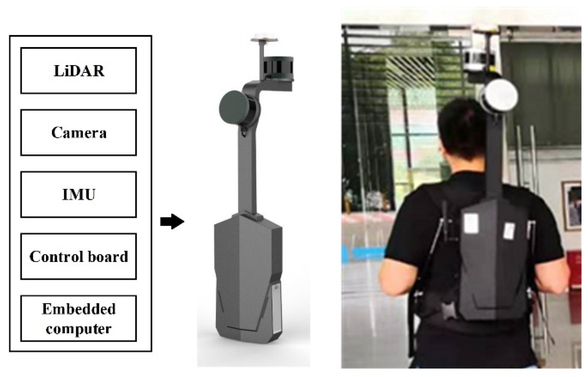
4.1. Equipment and Experimental Data

For large-scale 3D mapping applications in GNSS-denied environments, we develop a multisensor 3D MLS backpack mapping system (Figure 5). The system can collect high-precision time-synchronized IMU-LiDAR measurements. The system includes a KVH DSP-1750 fiber optic IMU and a Velodyne VLP-16 multiline LiDAR, and the sensors are integrated using an acquisition board to ensure time synchronization. The KVH DSP-1750 IMU is composed of three fiber optic gyroscopes and three MEMS accelerometers, and its sampling frequency is 250 Hz, so it can effectively capture the high-frequency motion of the carrier platform. The VLP-16 LiDAR scans the surrounding 360° environment at a frequency of approximately 10 Hz. In this paper, the point cloud obtained by a complete 360° scan is called a scan frame.

To verify the effectiveness of our method, we obtain the MLS measurement of the campus environment and buildings at Shenzhen University using a backpack system, and the test data include three different scenes: indoor, outdoor, and indoor-outdoor integrated. Our method is compared with the classic ICP, NICP [25] and IMU-aided ICP. The overall performance, accuracy and efficiency of our method are tested, which verifies the accuracy and reliability of our method.

4.2. Experimental Results

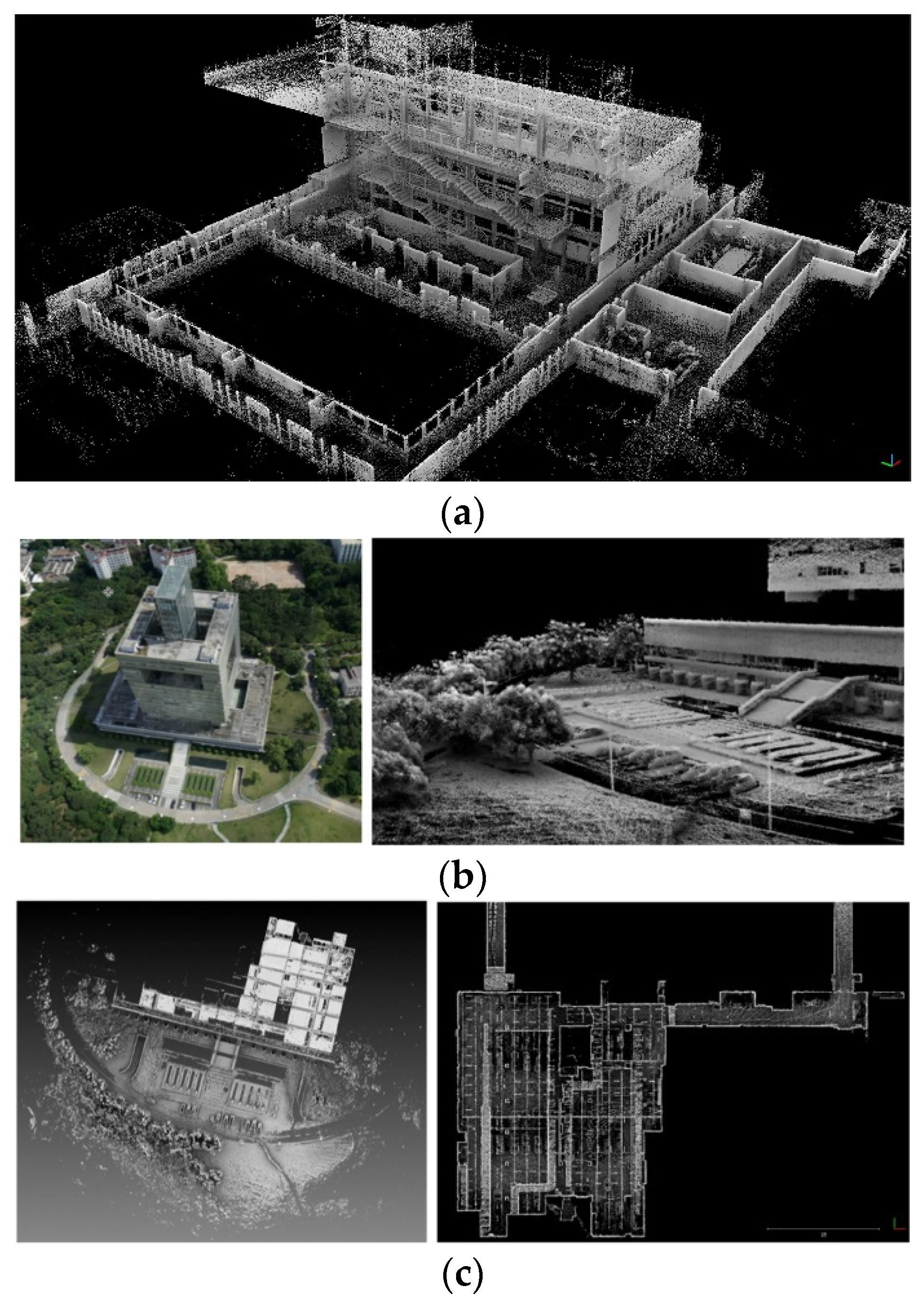
4.2.1. Indoor-Outdoor Mapping Application

Three typical scenes were selected: indoor, outdoor, and indoor-outdoor. Specifically, the indoor scene is an office building, the walking trajectory is from the 16th to 14th floors, and the indoor scene has many stairs. The outdoor scene walks around the office building, during which the surveyor passes through a lychee forest. In the indoor-outdoor scene, we start from the ground, pass through an underground parking lot, and then return to the starting point. The three scenes are shown in Figure 6.

Before data collection, the mapping system is static for 1–3 min, which is used for initialization. After data collection, a static alignment algorithm [40] is used to initialize the inertial navigation system, and then the proposed registration method is performed. Finally, the trajectory and point cloud map of the entire scene are obtained.

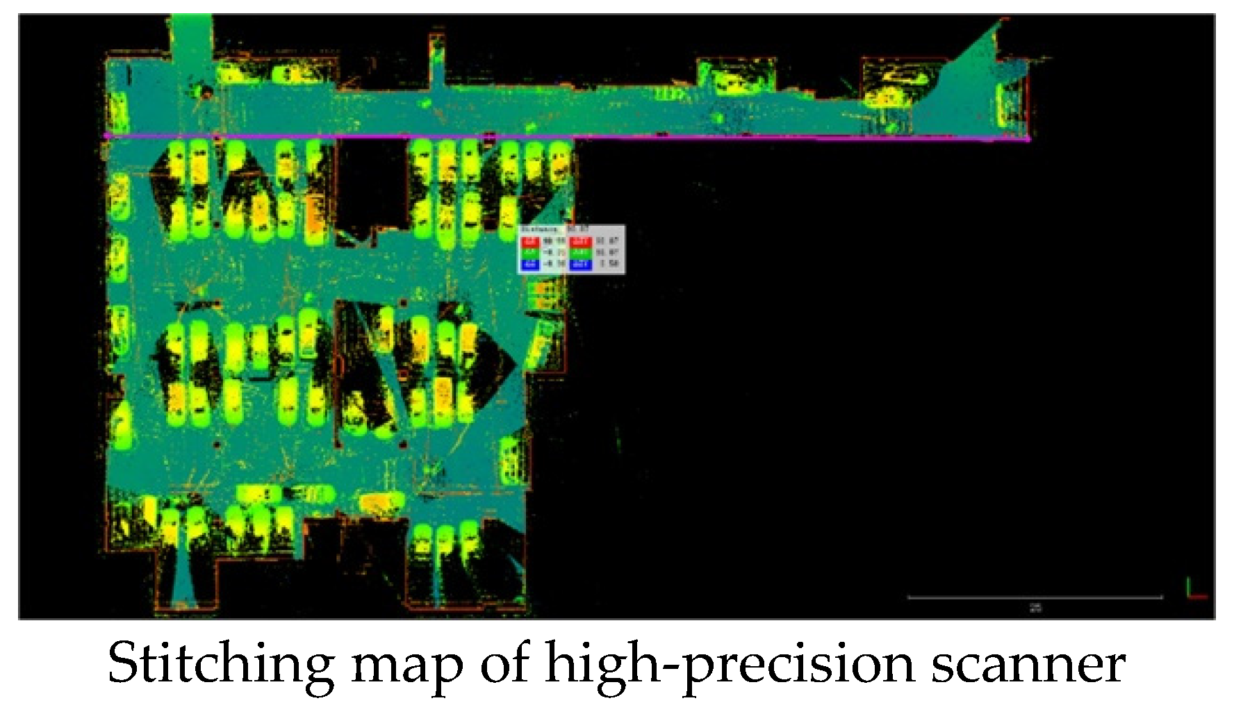
4.2.2. Mapping Accuracy

To verify the mapping accuracy, a typical indoor parking lot scene (approximately 100 m × 50 m) (in the indoor-outdoor integrated data) is selected and scanned with a high-precision ground scanner (Z+F5010 scanner). The range resolution of this scanner is 0.1 mm, and the range accuracy of the 50 m range is better than 2.2 mm. After multi-station scanning, the point cloud data are stitched and taken as ground-truth (Figure 7).

We first obtain a point cloud map using the proposed method, and then ICP registration is performed between the ground-truth and map of our method, thereby comparing the overall translation and rotation difference between them. A part of the wall distance is manually selected for plane accuracy comparison, and a part of the ground and ceiling feature points are selected for elevation accuracy comparison. The accuracy comparison is shown in

Table 1. Plane accuracy comparison.

Verification Distance	dours/m	dZ+F/m	ed/m
d1	46.05	46.08	−0.03
d2	14.7	14.65	0.05
d3	67.96	67.99	−0.03
d4	22.52	22.54	−0.02
d5	48.33	48.34	−0.01
d6	90.86	90.89	−0.03
d7	36.35	36.36	−0.01
RMSE			0.029

and

Table 2. Elevation accuracy comparison.

Verification Point	hours/m	hZ+F/m	eh/m
p1	−1.95	−1.92	−0.03
p2	−1.93	−1.92	−0.01
p3	−1.95	−1.93	−0.02
p4	−1.91	−1.95	0.04
p5	−1.93	−1.93	0.00
p6	−1.94	−1.95	0.01
p7	−1.93	−1.94	0.01
RMSE			0.021

. We select 7 wall distances and 7 points for accuracy verification, d_ours and h_ours represent the plane and elevation results of our method, d_Z+F and h_Z+F represent the ground-truth, and e_d and e_h represent the error. The results indicate that the plane accuracy of our method for the 100 m × 50 m indoor parking lot can reach 3 cm (1$\sigma$), and the elevation accuracy is approximately 2 cm (1$\sigma$), which meets the accuracy requirements of indoor 3D mapping.

4.2.3. Registration Algorithm Parameter Settings

In the proposed method, the key parameters are the number of scan frames in the point cloud window (window length, abbreviated as w) and the point cloud grid density (grid size, abbreviated as g). These two parameters directly affect the calculation efficiency. To test the influence of different parameters on the final generated map, four typical scenes were selected for the experiment (Figure 8), among which scene 1 was an indoor-outdoor transitional scene, scene 2 was an open indoor scene, scene 3 was an indoor scene in a narrow corridor, and scene 4 was an outdoor open scene.

By setting different parameters, submaps and trajectories within different periods of time can be obtained. We evaluated the influence of different parameters by comparing the trajectory difference after submap registration. As shown in Figure 9a, the maximum influence of parameter g on the trajectory is approximately 1.5 cm. Therefore, our method is insensitive to the choice of point cloud density. When accuracy requirement is not high, the density of the point cloud can be reduced to increase calculation speed.

To find the optimal setting of w, we select different window lengths for the IMU-LiDAR data fusion and obtain trajectories of different lengths. Taking the trajectory of the 80-frame window as a benchmark, we calculate the distance between trajectories of different window lengths and the benchmark, and the maximum difference is shown in Figure 9b. The trajectory error of different window lengths is stable within a certain parameter range, generally approximately 2 cm, and the maximum trajectory difference is 4 cm, which is equivalent to the range accuracy of the LiDAR, so the results indicate that the registration error is sensitive to different scenes rather than parameter settings.

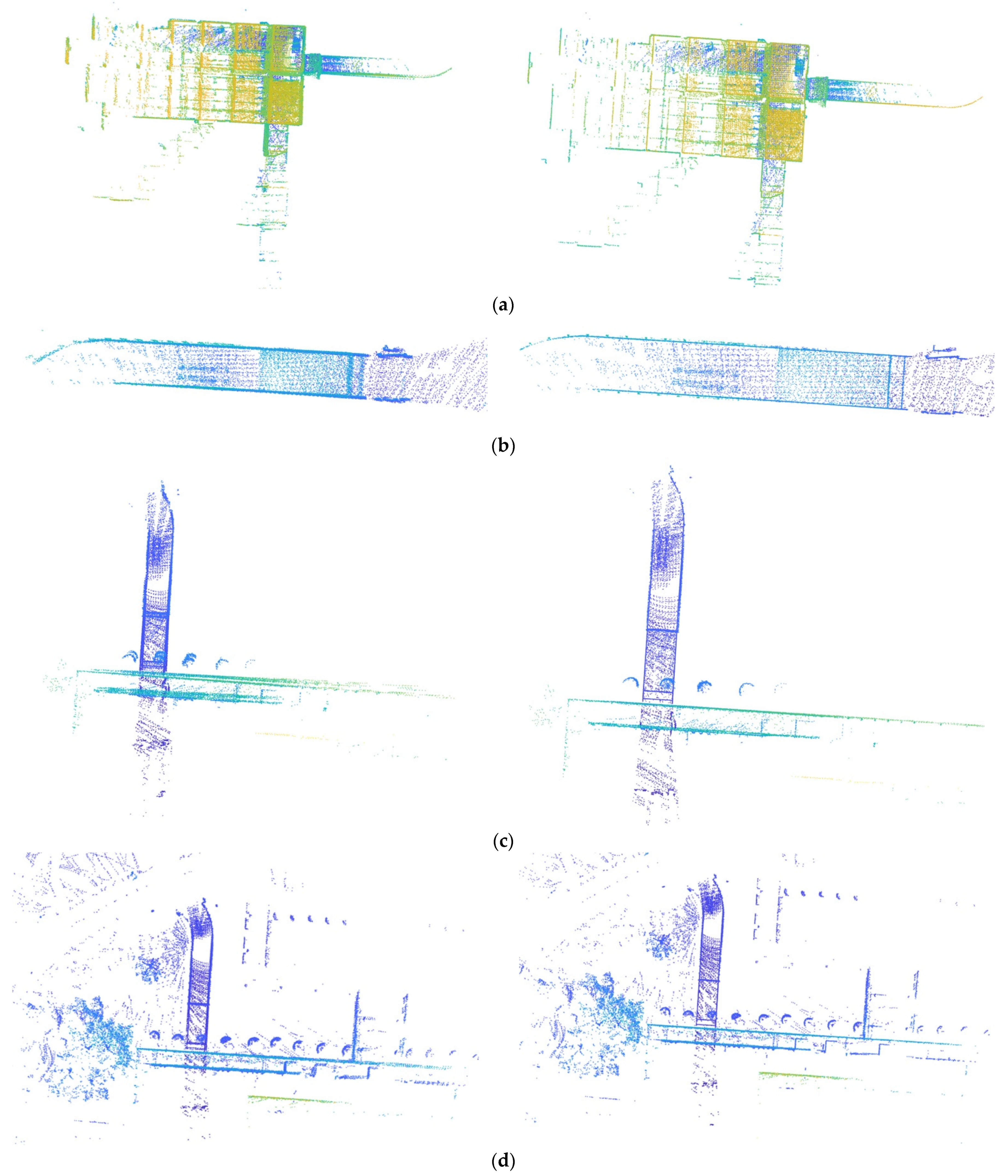
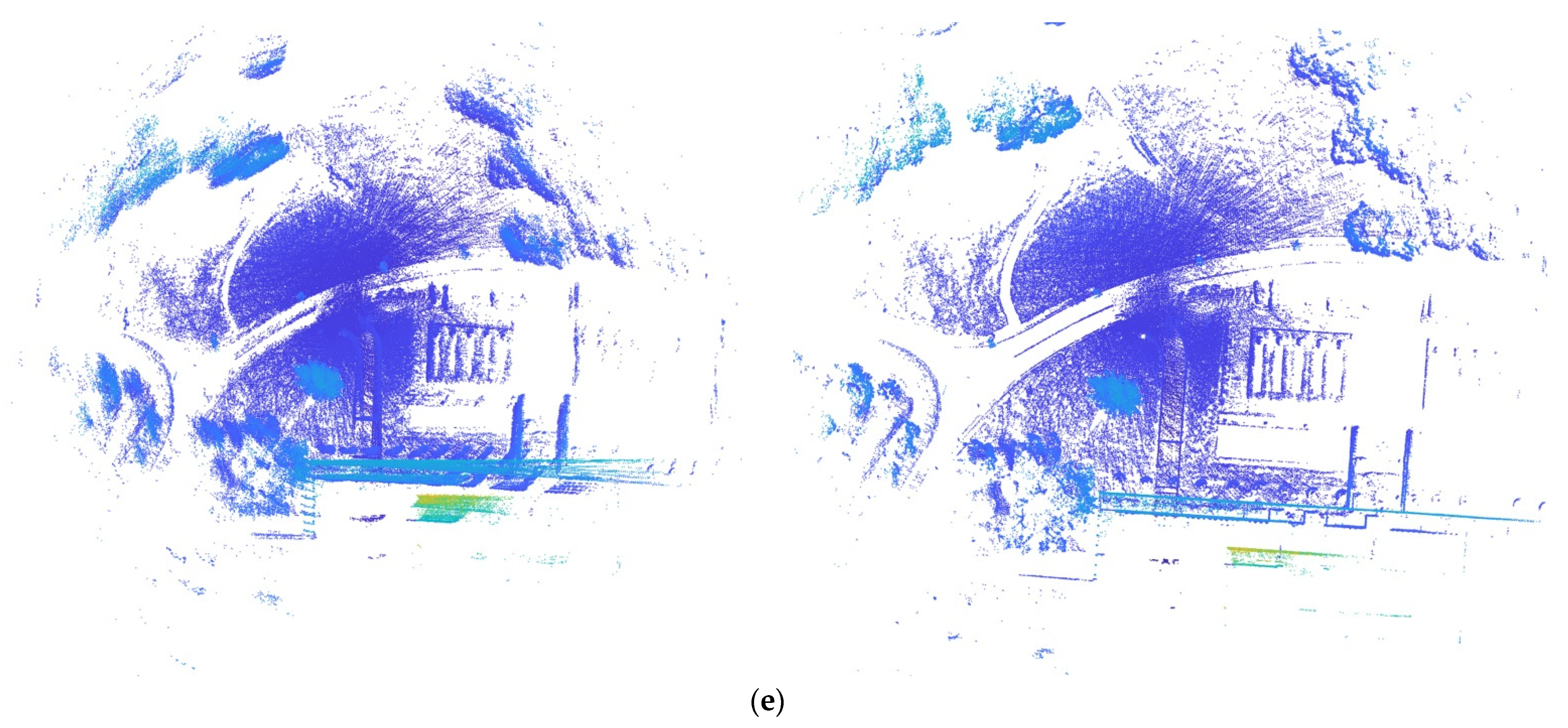
4.2.4. Registration Performance

Our method is compared with 3 methods to verify the registration accuracy and reliability: (1) The traditional ICP method. (2) NICP [25], an improved version of ICP that achieves state-of-the-art performance. (3) IMU-aided ICP, which also uses IMU to initially align point clouds, but then uses the ICP algorithm instead of our optimization model. The IMU-aided ICP experiment is used to illustrate the accuracy improvement of ICP with the assistance of IMU, and we can also compare the ICP iteration accuracy with the optimization accuracy of our method when both methods use IMU. Through the NICP experiment, it is shown that in the MLS registration task in complex environments, the proposed IMU-assisted registration method is more accurate than “LiDAR-only” registration method. Five typical scenes are selected from the indoor-outdoor integrated data for the experiment, among which scene 1 is an open indoor scene (41 frames), scene 2 is an underground passage indoor-outdoor scene (36 frames), scene 3 is a narrow corridor indoor scene (36 frames), scene 4 is a building outdoor scene (21 frames), and scene 5 is an outdoor open scene (100 frames). In the experiment, the outlier removal ratio [41] of the ICP method was set to 0.2. The meaning of this parameter is to reject a given percentage of the worst point pairs based on their Euclidean distance.

The evaluation metrics we chose referred to [9]. The most intuitive metric for point cloud registration is visual evaluation. For data with ground-truth such as control points or true poses, the errors of control points coordinates are compared, or the rotation error and translation error between scan frames are calculated. However, in some real-world mapping tasks, it is difficult to obtain ground-truth, which makes it impossible to use the above metrics based on the ground-truth. In this case, without a ground-truth, the root mean square (RMS) of the correspondence distance is usually used as a metric.

In this paper, we select RMS as the evaluation metric for registration accuracy, and we use visual evaluation of the registration result as a supplement. In addition, through comparison of the operating time, we test the efficiency and practicability of our method.

• Registration accuracy

We first compare the registration accuracy between two adjacent frames. In the above five scenes, two adjacent frames of the point clouds are selected for registration, and the RMS is calculated (Equations (13) and (14)). It should be noted that in the traditional ICP method, the error is large without providing initial estimates, and the ICP method fails to converge. In contrast, our performance is good due to the assistance of the IMU. Due to the above situation, to make a quantitative comparison, we use the initial IMU integration trajectory as the initial estimates for the ICP method and then compare the ICP method with accurate initial estimates and our method.

$$RMS=\sqrt{\frac{{{\displaystyle \sum }}_{i=1}^N{\left[\mathit{d}\left({\mathit{p}}_i,{\mathit{q}}_i{}^{\prime }\right)\right]}^2}{N}}$$

(13)

$$\mathit{d}\left({\mathit{p}}_i,{\mathit{q}}_i{}^{\prime }\right)=\Vert {\mathit{p}}_i-\left(\mathit{R}·{\mathit{q}}_i+\mathit{T}\right)\Vert =\sqrt{{\left(x_{p_i}-x_{q_i}^{\prime }\right)}^2+{\left(y_{p_i}-y_{q_i}^{\prime }\right)}^2+{\left(z_{p_i}-z_{q_i}^{\prime }\right)}^2}$$

(14)

where ${\mathit{p}}_i,{\mathit{q}}_i$ are correspondences obtained by registration between scan frames $\left(\mathit{p},\mathit{q}\right)$, (R, T) represents the estimated relative pose after registration and $\mathit{d}\left({\mathit{p}}_i,{\mathit{q}}_i\right)$ represents the Euclidean distance between correspondences. The results of registration accuracy are shown in

Table 3. Registration accuracy comparison.

Method	Scene 1 RMS	Scene 2 RMS	Scene 3 RMS	Scene 4 RMS	Scene 5 RMS
ICP	0.272 m	0.164 m	0.586 m	0.671 m	0.692 m
NICP	0.206 m	0.154 m	0.470 m	0.453 m	0.526 m
IMU-aided ICP	0.177 m	0.134 m	0.193 m	0.289 m	0.405 m
Our method	0.155 m	0.123 m	0.178 m	0.258 m	0.367 m

.

By comparing the RMS of the same scene, it can be seen that the accuracy of our method is superior to other 3 methods. Compared with the IMU-aided ICP, our method achieves higher accuracy. The comparison with ICP and NICP methods further demonstrates the improvement of the registration accuracy with the assistance of the IMU. Through the comparison between different scenes, the indoor RMS error is better than outdoor scenes. On the one hand, indoor scenes have richer structures and features, and objects in outdoor scenes contain homogeneous structures. In addition, obstacles such as trees will cause occlusion, which affects the registration accuracy. On the other hand, a point cloud is relatively sparse in an outdoor scene, so the distance between correspondences will increase accordingly. As a result, the RMS based on distance will be relatively large.

2.

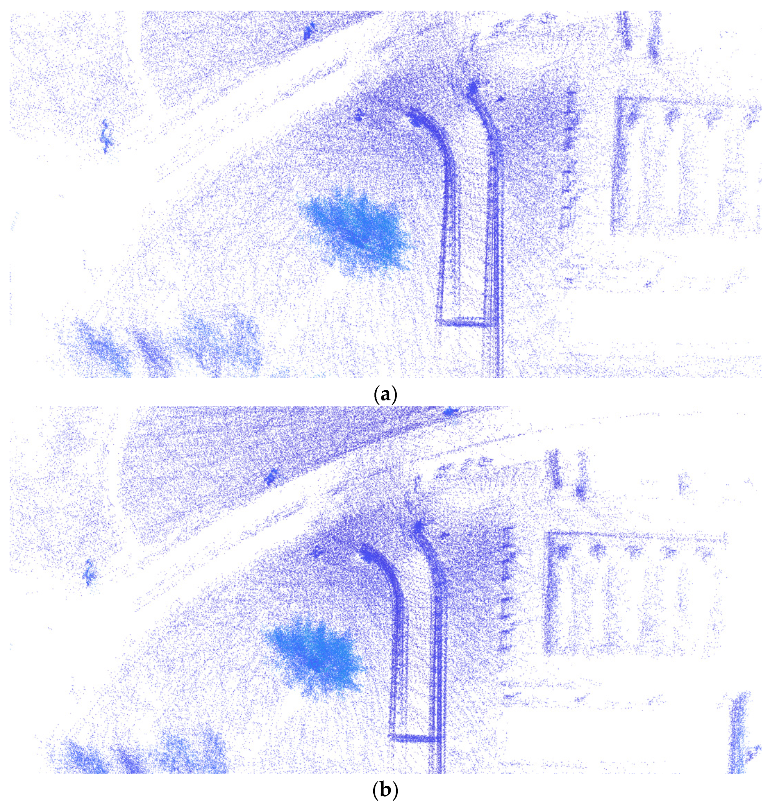
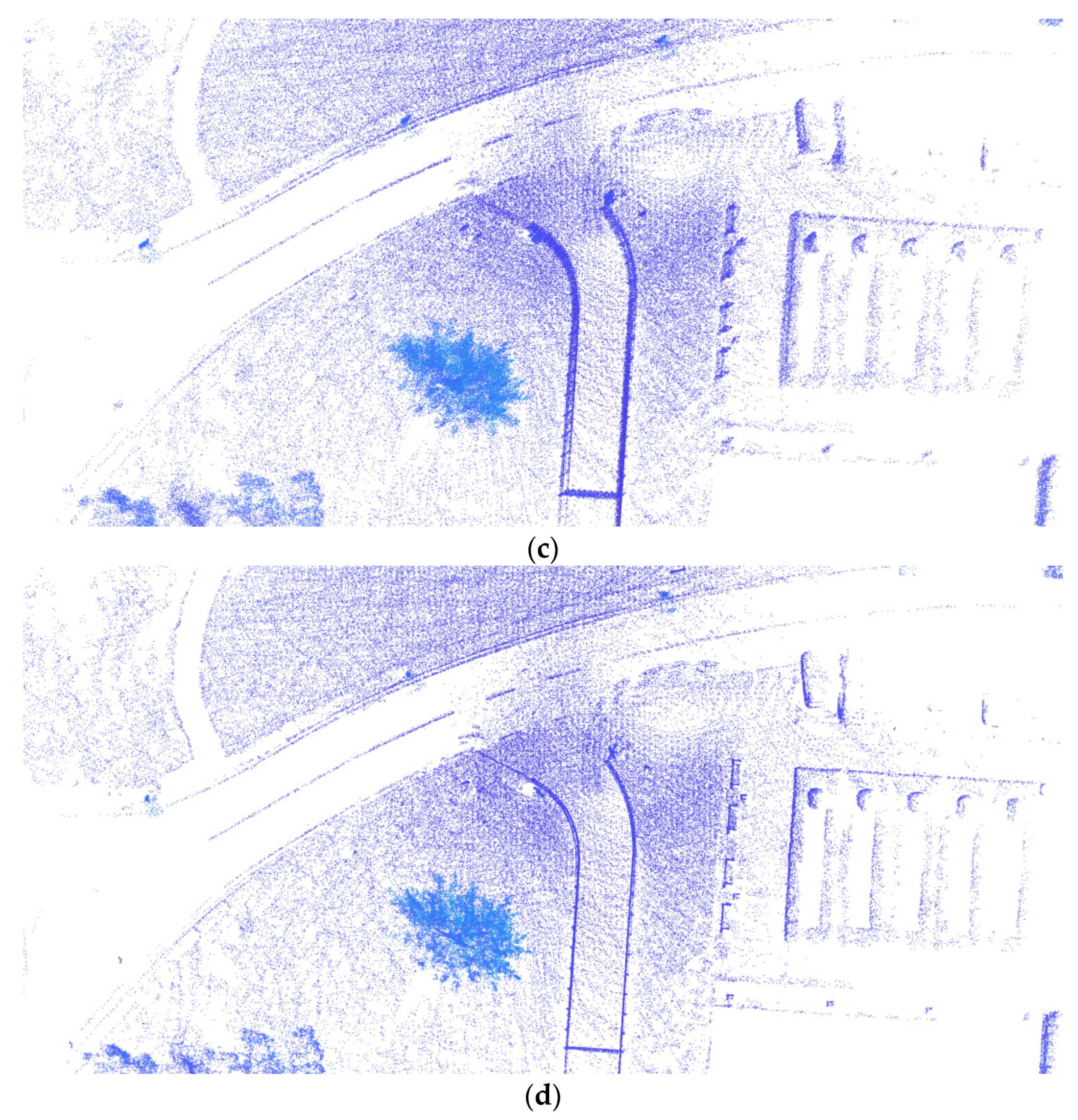
Visual evaluation of local submaps

After continuous registration, the sequence point cloud is fused with the estimated trajectory to generate a submap, and then we compare the visual performance of the submap based on point cloud registration. This comparison aims to verify the reliability of our method for continuous registration. The results of the submaps show that there are obvious dislocations in the ICP submaps, especially in outdoor scenes 4 and 5, such as trees, roads and buildings, and the submaps of our method are significantly better than those of the ICP method.

By visually comparing the submaps, the superiority of our method in sequence point cloud registration is demonstrated, and the accuracy and robustness of our method in a variety of complex scenarios are proven. Figure 10 shows the overall performance of the 5 scenes. In Figure 11, local areas in scene 5 with obvious contrast are selected for magnification to visually demonstrate the superiority of our method.

3.

Efficiency

For real-world 3D mapping tasks, efficiency is also a key metric. By counting the operating time for the sequence registration of 300 scan frames, we compare the efficiency of our method with other 3 methods. The average number of points per point cloud frame is 13,886. The code of the methods are all MATLAB versions, and the experiment runs on a laptop equipped with an Intel i7-10875H CPU. To finish the registration of 300-frame sequence point clouds, the ICP method takes 80.54 s, the NICP method takes 63.25 s, the IMU-aided ICP takes 22.86 s, and our method takes 28.05 s. The running time of the ICP method is approximately 3 times that of our method.

The results of efficiency experiment are shown in

Table 4. Comparison of operating time for 300-frame registration.

Method	Running Time/Seconds
ICP	80.54
NICP	63.25
IMU-aided ICP	22.86
Our method	28.05

. Compared with ICP and NICP, the efficiency improvement of our method lies in the assistance of the IMU. Our method provides a more accurate initial estimation to assist the nearest neighbor search through the constraints of the short time period inertial trajectory, thereby speeding up the convergence. Compared with IMU-aided ICP, our method utilizes the IMU assistance in each loop, which improving the efficiency; while in IMU-aided ICP, the IMU does not participate in the iterations, so the convergence speed of our method is faster. The results indicate that our method has good efficiency and practicability in 3D mapping tasks.

5. Discussion

In this section, we explain the environmental adaptability of our method and discuss the practicality and limitations.

In terms of environmental adaptability, our method is suitable for indoor-outdoor integrated scenes and indoor scenes. In these GNSS-denied scenarios, point cloud registration is prone to be fragile. Facing this situation, an IMU can provide stable motion measurements. The proposed inertial trajectory error model builds constraints between multiple scan frames in a short time window and optimizes multiple frames in the window, so our method can effectively avoid the impact of matching failures (due to structural repetition, occlusion or moving objects) and improve the accuracy and robustness of point cloud registration. In an open outdoor scene, because the GNSS signal is good, it can provide an absolute position to directly constrain the point cloud, so IMU can be replaced by GNSS.

In terms of practicality, the main advantage of our method is modularity. Compared to tightly-coupled LiDAR-IMU methods, our method can serve as a separate registration submodule and can be easily extended to other multisource navigation frameworks. Instead of simply using inertial pose as a priori, we establish a model between the inertial error and point cloud error. On the one hand, we use an error model of an inertial trajectory over a short time period to constrain the point cloud registration error and optimize it using the least squares method, which directly improves the accuracy of registration. On the other hand, the optimization result can be fed back to update the inertial trajectory, thus establishing a two-way optimization between the IMU and LiDAR. On this basis, by adding this model to a Kalman filter or optimization-based methods, our method can be easily extended to a LiDAR-inertial odometer and can further serve as a LiDAR-inertial submodule for multisource data fusion.

The limitation of our method is that the registration accuracy is affected by the performance of the IMU itself, which means that the parameter of time window length (window length, w) needs to be adjusted according to actual situations. This is because when we estimate the inertial trajectory error model parameters (Section 3.2), we put forward the following assumption: in Equation (8), we combine $-{\left[\mathit{\theta }\right]}_{\times }{\widehat{\mathit{C}}}_b^{\mathit{C}}{\widehat{\mathit{p}}}^b$ and ${\widehat{\mathit{C}}}_b^n\delta {\mathit{p}}^b$ into a random error. The reason for this assumption is that the attitude error caused by the IMU gyro bias over a short time period is very small, so it only has a minimal effect on LiDAR with centimeter-level measurement noise. When the accuracy of the IMU is high, this assumption will be valid in a relatively longer time window, so the window length w can be set larger. When a low-cost IMU is used, since the IMU error diverges faster, to ensure that the proposed assumption is valid, a smaller window length w should be set, otherwise the accuracy will decrease when the IMU gyro bias become large. Due to the limitations of our experimental conditions, in Section 4.2.3 we only discuss parameter settings of high-precision IMU, and we do not analyze the situation when using a low-cost IMU. Therefore, to obtain better performance, we recommend that readers use high-precision IMU when applying our method. If a low-cost IMU is used, the parameter settings should be adjusted according to actual situation. In the future, we will continue to research and optimize the proposed IMU trajectory error model to improve its practicality.

6. Conclusions

Achieving efficient and reliable MLS point cloud registration in complex environments is a research hotspot in the fields of 3D mapping and inspection, SLAM and robotics. Aiming at this problem, we propose an inertial trajectory error model over a short time period to construct constraints for point cloud registration, minimize the point cloud error through least squares optimization, and achieve reliable MLS point cloud registration.

The contribution of this paper is mainly reflected in three aspects. (1) We propose an inertial trajectory error model over a short time period, which constructs motion constraints between different scan frames in a short time window. (2) An inertial-aided MLS point cloud registration method is proposed, we optimize the inertial trajectory error model parameters and point cloud registration errors at the same time, and realize continuous MLS point cloud registration, which has the advantage of high accuracy, simplicity, and extendibility. (3) We propose a cross-matching strategy to ensure high-overlap between point clouds and effectively improve the registration reliability. We develop a multisensor 3D MLS backpack mapping system to collect data in campus environments and conduct detailed comparative experiments in various scenes. In terms of mapping accuracy, the RMSE of plane accuracy is 0.029 m, the RMSE of elevation accuracy is 0.021 m. The frame-to-frame registration accuracy of our method reaches sub-meter, and the running time for 300-frame registration is 28.05 s. The experimental results prove the superiority of our method in complex environments.

Although our method has the limitation that the registration accuracy is affected by the device errors of the IMU, it has good practicality for solving 3D mapping tasks. In the future, we will further research registration methods and try to solve the limitations of this method. The LiDAR-inertial fusion problem has broad application prospects and room for improvement, and we hope this article will provide help for future research.

References

1. Dong, Z.; Liang, F.; Yang, B.; Xu, Y.; Zang, Y.; Li, J.; Wang, Y.; Dai, W.; Fan, H.; Hyyppä, J.; et al. Registration of large-scale terrestrial laser scanner point clouds: A review and benchmark. ISPRS J. Photogramm. Remote Sens. 2020, 163, 327–342. [Google Scholar] [CrossRef]
2. Cheng, L.; Chen, S.; Liu, X.; Xu, H.; Wu, Y.; Li, M.; Chen, Y. Registration of Laser Scanning Point Clouds: A Review. Sensors 2018, 18, 1641. [Google Scholar] [CrossRef] [PubMed] [Green Version]
3. Tam, G.K.L.; Cheng, Z.-Q.; Lai, Y.-K.; Langbein, F.; Liu, Y.; Marshall, D.; Martin, R.R.; Sun, X.; Rosin, P. Registration of 3D Point Clouds and Meshes: A Survey from Rigid to Nonrigid. IEEE Trans. Visual. Comput. Graph. 2013, 19, 1199–1217. [Google Scholar] [CrossRef] [PubMed] [Green Version]
4. Paneque, J.L.; Dios, J.R.M.; Ollero, A. Multi-Sensor 6-DoF Localization for Aerial Robots in Complex GNSS-Denied Environments. In Proceedings of the 2019 IEEE/RSJ International Conference on Intelligent Robots and Systems (IROS), Macau, China, 3–8 November 2019; pp. 1978–1984. [Google Scholar] [CrossRef]
5. Huang, R.; Xu, Y.; Yao, W.; Hoegner, L.; Stilla, U. Robust global registration of point clouds by closed-form solution in the frequency domain. ISPRS J. Photogramm. Remote Sens. 2021, 171, 310–329. [Google Scholar] [CrossRef]
6. Besl, P.J.; McKay, N.D. A method for registration of 3-D shapes. IEEE Trans. Pattern Anal. Mach. Intell. 1992, 14, 239–256. [Google Scholar] [CrossRef]
7. Aiger, D.; Mitra, N.J.; Cohen-Or, D. 4-points Congruent Sets for Robust Pairwise Surface Registration. ACM Trans. Graph. 2008, 27, 10. [Google Scholar] [CrossRef] [Green Version]
8. Charles, R.Q.; Su, H.; Kaichun, M.; Guibas, L.J. PointNet: Deep Learning on Point Sets for 3D Classification and Segmentation. In Proceedings of the 2017 IEEE Conference on Computer Vision and Pattern Recognition (CVPR), Honolulu, HI, USA, 21–26 July 2017; pp. 77–85. [Google Scholar] [CrossRef] [Green Version]
9. Nguyen, H.L.; Belton, D.; Helmholz, P. Review of mobile laser scanning target-free registration methods for urban areas using improved error metrics. Photogram Rec. 2019, 34, 282–303. [Google Scholar] [CrossRef]
10. Yan, L.; Tan, J.; Liu, H.; Xie, H.; Chen, C. Automatic non-rigid registration of multi-strip point clouds from mobile laser scanning systems. Int. J. Remote Sens. 2018, 39, 1713–1728. [Google Scholar] [CrossRef]
11. Zhang, Y.; Xiong, X.; Zheng, M.; Huang, X. LiDAR Strip Adjustment Using Multifeatures Matched With Aerial Images. IEEE Trans. Geosci. Remote Sens. 2015, 53, 976–987. [Google Scholar] [CrossRef]
12. Wendt, A. A concept for feature based data registration by simultaneous consideration of laser scanner data and photogrammetric images. ISPRS J. Photogramm. Remote Sens. 2007, 62, 122–134. [Google Scholar] [CrossRef]
13. Han, J.-Y.; Perng, N.-H.; Chen, H.-J. LiDAR Point Cloud Registration by Image Detection Technique. IEEE Geosci. Remote Sens. Lett. 2013, 10, 746–750. [Google Scholar] [CrossRef]
14. Abayowa, B.O.; Yilmaz, A.; Hardie, R.C. Automatic registration of optical aerial imagery to a LiDAR point cloud for generation of city models. ISPRS J. Photogramm. Remote Sens. 2015, 106, 68–81. [Google Scholar] [CrossRef]
15. Gobakken, T.; Næsset, E. Assessing effects of positioning errors and sample plot size on biophysical stand properties derived from airborne laser scanner data. Can. J. For. Res. 2009, 39, 1036–1052. [Google Scholar] [CrossRef]
16. Shan, T.; Englot, B.; Ratti, C.; Rus, D. LVI-SAM: Tightly-Coupled Lidar-Visual-Inertial Odometry via Smoothing and Mapping. arXiv 2021, arXiv:2104.10831. [Google Scholar]
17. Gressin, A.; Cannelle, B.; Mallet, C.; Papelard, J.-P. Trajectory-Based Registration of 3D Lidar Point Clouds Acquired with a Mobile Mapping System. ISPRS Ann. Photogramm. Remote Sens. Spatial Inf. Sci. 2012, I-3, 117–122. [Google Scholar] [CrossRef] [Green Version]
18. Takai, S.; Date, H.; Kanai, S.; Niina, Y.; Oda, K.; Ikeda, T. Accurate registration of MMS point clouds of urban areas using trajectory. ISPRS Ann. Photogramm. Remote Sens. Spatial Inf. Sci. 2013, II-5/W2, 277–282. [Google Scholar] [CrossRef] [Green Version]
19. Qin, T.; Li, P.; Shen, S. VINS-Mono: A Robust and Versatile Monocular Visual-Inertial State Estimator. IEEE Trans. Robot. 2018, 34, 1004–1020. [Google Scholar] [CrossRef] [Green Version]
20. Shan, T.; Englot, B.; Meyers, D.; Wang, W.; Ratti, C.; Rus, D. LIO-SAM: Tightly-Coupled Lidar Inertial Odometry via Smoothing and Mapping. arXiv 2020, arXiv:2007.00258. [Google Scholar]
21. Zhao, S.; Zhang, H.; Wang, P.; Nogueira, L.; Scherer, S. Super Odometry: IMU-Centric LiDAR-Visual-Inertial Estimator for Challenging Environments. arXiv 2021, arXiv:2104.14938. [Google Scholar]
22. Bae, K.-H.; Lichti, D.D. A method for automated registration of unorganised point clouds. ISPRS J. Photogramm. Remote Sens. 2008, 63, 36–54. [Google Scholar] [CrossRef]
23. Chetverikov, D.; Svirko, D.; Stepanov, D.; Krsek, P. The Trimmed Iterative Closest Point algorithm. In Proceedings of the Object Recognition Supported by User Interaction for Service Robots, Quebec City, QC, Canada, 11–15 August 2002; Volume 3, pp. 545–548. [Google Scholar] [CrossRef]
24. Pavlov, A.L.; Ovchinnikov, G.W.V.; Derbyshev, D.Y.; Tsetserukou, D.; Oseledets, I.V. AA-ICP: Iterative Closest Point with Anderson Acceleration. In Proceedings of the 2018 IEEE International Conference on Robotics and Automation (ICRA), Brisbane, QLD, Australia, 21–25 May 2018; pp. 3407–3412. [Google Scholar] [CrossRef] [Green Version]
25. Serafin, J.; Grisetti, G. NICP: Dense Normal Based Point Cloud Registration. In Proceedings of the 2015 IEEE/RSJ International Conference on Intelligent Robots and Systems (IROS), Hamburg, Germany, 28 September–2 October 2015; pp. 742–749. [Google Scholar] [CrossRef] [Green Version]
26. Rusu, R.B.; Blodow, N.; Beetz, M. Fast Point Feature Histograms (FPFH) for 3D Registration. In Proceedings of the 2009 IEEE International Conference on Robotics and Automation, Kobe, Japan, 12–17 May 2009; pp. 3212–3217. [Google Scholar] [CrossRef]
27. Guo, Y.; Sohel, F.; Bennamoun, M.; Lu, M.; Wan, J. Rotational Projection Statistics for 3D Local Surface Description and Object Recognition. Int. J. Comput. Vis. 2013, 105, 63–86. [Google Scholar] [CrossRef] [Green Version]
28. Salti, S.; Tombari, F.; di Stefano, L. SHOT: Unique signatures of histograms for surface and texture description. Comput. Vis. Image Underst. 2014, 125, 251–264. [Google Scholar] [CrossRef]
29. Qi, C.R.; Yi, L.; Su, H.; Guibas, L.J. PointNet++: Deep Hierarchical Feature Learning on Point Sets in a Metric Space. arXiv 2017, arXiv:1706.02413. [Google Scholar]
30. Aoki, Y.; Goforth, H.; Srivatsan, R.A.; Lucey, S. PointNetLK: Robust & Efficient Point Cloud Registration Using PointNet. In Proceedings of the 2019 IEEE/CVF Conference on Computer Vision and Pattern Recognition (CVPR), Long Beach, CA, USA, 15–20 June 2019; pp. 7156–7165. [Google Scholar] [CrossRef] [Green Version]
31. Forster, C.; Carlone, L.; Dellaert, F.; Scaramuzza, D. On-Manifold Preintegration for Real-Time Visual—Inertial Odometry. IEEE Trans. Robot. 2017, 33, 1–21. [Google Scholar] [CrossRef] [Green Version]
32. Wu, J. MARG Attitude Estimation Using Gradient-Descent Linear Kalman Filter. IEEE Trans. Automat. Sci. Eng. 2020, 17, 1777–1790. [Google Scholar] [CrossRef]
33. Wu, J.; Zhang, S.; Zhu, Y.; Getng, R.; Fu, Z.; Ma, F.; Liu, M. Differential Information Aided 3-D Registration for Accurate Navigation and Scene Reconstruction. In Proceedings of the 2021 IEEE International Conference on Robotics and Automation (ICRA), Xi’an, China, 30 May–5 June 2021; pp. 9249–9254. [Google Scholar] [CrossRef]
34. Zhang, J.; Singh, S. Low-drift and real-time lidar odometry and mapping. Auton. Robot. 2017, 41, 401–416. [Google Scholar] [CrossRef]
35. Gentil, C.L.; Vidal-Calleja, T.; Huang, S. IN2LAMA: INertial Lidar Localisation And MApping. In Proceedings of the 2019 International Conference on Robotics and Automation (ICRA), Montreal, QC, Canada, 20–24 May 2019; pp. 6388–6394. [Google Scholar] [CrossRef]
36. Bosse, M.; Zlot, R.; Flick, P. Zebedee: Design of a Spring-Mounted 3-D Range Sensor with Application to Mobile Mapping. IEEE Trans. Robot. 2012, 28, 1104–1119. [Google Scholar] [CrossRef]
37. Xu, W.; Zhang, F. FAST-LIO: A Fast, Robust LiDAR-inertial Odometry Package by Tightly-Coupled Iterated Kalman Filter. arXiv 2021, arXiv:2010.08196. [Google Scholar] [CrossRef]
38. Qin, C.; Ye, H.; Pranata, C.E.; Han, J.; Zhang, S.; Liu, M. LINS: A Lidar-Inertial State Estimator for Robust and Efficient Navigation. In Proceedings of the 2020 IEEE International Conference on Robotics and Automation (ICRA), Paris, France, 31 May–31 August 2020; pp. 8899–8906. [Google Scholar] [CrossRef]
39. Zhang, J.; Singh, S. Laser-visual-inertial odometry and mapping with high robustness and low drift. J. Field Robot. 2018, 35, 1242–1264. [Google Scholar] [CrossRef]
40. Shin, E.H. Estimation Techniques for Low-Cost Inertial Navigation. In UCGE Report; University of Calgary: Calgary, AB, Canada, 2005. [Google Scholar]
41. Pomerleau, F.; Colas, F.; Siegwart, R. A Review of Point Cloud Registration Algorithms for Mobile Robotics. Found. Trends Robot. 2015, 4, 1–104. [Google Scholar] [CrossRef] [Green Version]
Figure 1. LiDAR-IMU measurement system.
Remotesensing 14 01365 g001
Figure 2. Inertial-aided mobile LiDAR scanning point cloud registration method.
Remotesensing 14 01365 g002
Figure 3. Flow chart of the proposed method.
Remotesensing 14 01365 g003
Figure 4. Continuous cross-matching strategy.
Remotesensing 14 01365 g004
Figure 5. Multisensor 3D MLS backpack mapping system.
Remotesensing 14 01365 g005
Figure 6. Experimental scenes. (a) The indoor scene. (b) The outdoor scene. (c) The indoor-outdoor integrated scene.
Remotesensing 14 01365 g006
Figure 7. The ground-truth of indoor 3D map.
Remotesensing 14 01365 g007
Figure 8. Four typical scenes for the parameter comparison experiment. (a) Indoor-outdoor transitional scene. (b) Open indoor scene. (c) Indoor scene in a narrow corridor. (d) Outdoor open scene.
Remotesensing 14 01365 g008
Figure 9. The influence of parameters on the trajectory. (a) grid size g. (b) window length w.
Remotesensing 14 01365 g009aRemotesensing 14 01365 g009b
Figure 10. Sequence point cloud registration submaps. The left column shows the submap of ICP in 5 scenes, the right column shows the submap of our method. The 5 rows represent 5 scenes: (a) Open indoor; (b) Indoor-outdoor scene of an underground passage; (c) Indoor narrow corridor; (d) Outdoor building; (e) Outdoor open scene.
Remotesensing 14 01365 g010aRemotesensing 14 01365 g010b
Figure 11. Comparison of a local magnification of the submaps in scene 5. (a) The local magnification of the submap in scene 5 with the ICP method. (b) The local magnification of the submap in scene 5 with the NICP method. (c) The local magnification of the submap in scene 5 with the IMU-aided ICP method. (d) The local magnification of the submap in scene 5 with our method.
Remotesensing 14 01365 g011aRemotesensing 14 01365 g011b