Article

Estimating Species-Specific Stem Size Distributions of Uneven-Aged Mixed Deciduous Forests Using ALS Data and Neural Networks

TERRA Teaching and Research Centre—Forest Is Life, University of Liège (Uliège)—Gembloux Agro-Bio Tech, 5030 Gembloux, Belgium
*
Author to whom correspondence should be addressed.
Remote Sens. 2022, 14(6), 1362; https://doi.org/10.3390/rs14061362
Submission received: 10 February 2022 / Revised: 8 March 2022 / Accepted: 9 March 2022 / Published: 11 March 2022
(This article belongs to the Special Issue Advances in LiDAR Remote Sensing for Forestry and Ecology)

Abstract

:
Sustainable forest management requires accurate fine-scale description of wood resources. Stem size distribution (SSD) by species is used by foresters worldwide as a representative overview of forest structure and species composition suitable for informing management decisions at shorter and longer terms. In mixed uneven-aged deciduous forests, tree data required for SSD estimation are most often collected in the field through traditional forest management inventories (FMIs), but these are time-consuming and costly with respect to the sampled area. Combining FMIs with remote sensing methods such as airborne laser scanning (ALS), which has high potential for predicting forest structure and composition, and is becoming increasingly accessible and affordable, could provide cheaper and faster SSD data across large areas. In this study, we developed a method for estimating species-specific SSDs by combining FMIs and dual-wavelength ALS data using neural networks (NNs). The proposed method was tested and validated using 178 FMI plots within 22,000 ha of a mixed uneven-aged deciduous forest in Belgium. The forest canopy was segmented, and metrics were derived from the ALS point cloud. A NN with a custom architecture was set up to simultaneously predict the three components required to compute species-specific SSDs (species, circumference, and number of stems) at segment level. Species-specific SSDs were thereafter estimated at stand level by aggregating the estimates for the segments. A robustness test was set up using fully independent plots to thoroughly assess the method precision at stand-level on a larger area. The global Reynolds index for the species-specific SSDs was 21.2 for the training dataset and 54.0 for the independent dataset. The proposed method does not require allometric models, prior knowledge of the structure, or the predefinition of variables; it is versatile and thus potentially adaptable to other forest types having different structures and compositions.

1. Introduction

Sustainable forest management requires a detailed and accurate description of forest resources [1]. Species-specific stem-size distribution (SSD) is a critical variable for evaluating forests in terms of structure and species composition, especially in uneven-aged stands [2,3]. The tree measurement most often used by foresters to construct SSD is the diameter or, more rarely (as is the case in Belgium), the circumference. SSD allows the assessment of forest regeneration state [4] and mature tree proportion [2], depending on inventory threshold and stem-size class width. Depending on forest type and management objectives, this allows to check the balance state and, if necessary, adjust silviculture, plan interventions, and appraise timber harvesting [5]. SSD is usually interpreted graphically by species with the y- and x-axes corresponding to stem density and stem-size classes, respectively. Comparison of SSD at different times is also a relevant indicator of stand evolution [6], while mathematical relations and allometric models also allow the use of SSD to express major stand parameters such as total basal area, wood volume, and biomass. The species-specific SSD is therefore an important data for describing structure and composition of forests.
Although some countries (Norway, Finland, Sweden, Denmark) use airborne laser scanning (ALS) to inventory forests at a large scale [7,8,9], most traditional forest management inventories (FMI) rely on data collected in the field; in particular, for SSD estimation at management unit level (i.e., forest stand or property rather than single plot) in mixed uneven-aged deciduous forests. Such field data are used to adjust forest management practices and to draw up management plans [10,11]. Considering uneven-aged forests, field data most often correspond to sample-based inventories [12] and tree data are collected on plots generally located on a regular grid [13]. For instance, in Belgium, the sampling rate is usually one plot per 1–10 ha. The sampling rate needs to be adapted according to the expected precision [12,14]. In even-aged forests, traditional FMI data correspond to stand variables like volume, basal area, average size or dominant height estimated using visual assessment or relascope measurements [7]. In mixed uneven-aged forests, main measurements cover variables including individual tree dendrometric variables (e.g., circumference and height) and regeneration measurements (e.g., coverage of developmental stages) depending on management objectives and constraints [10,11,15]. For management purposes, FMI data only make sense if they are aggregated at the stand or forest level. Traditional FMI are therefore frequent and widespread for uneven-aged deciduous forests and could be used to estimate SSD.
Since the early 2000s, a great deal of interest was put on SSD estimation using ALS data. Firstly, this interest was focused on boreal forests and plantations of primarily coniferous species. The area based approaches (ABA) were used with either non-parametric modelling, such as the k-nearest neighbor method (kNN) [16,17,18,19,20,21,22], or parametric modelling considering the Weibull distribution for plantations [23,24,25,26] and even-aged stands [27,28,29,30,31]. In more complex stands, plots were differentiated based on modality (unimodal or bimodal) before the prediction of distribution parameters (shape and scale) [32]. The individual tree detection (ITD) approaches were also implemented to estimate the SSD. Tree diameter at breast height (DBH) has been estimated using several DBH regression models corresponding to different growth patterns which integrated segment properties, forest density, and local topography [33]. Machine learning techniques were also used to predict individual tree DBH [34]. The ABA and ITD approaches were also combined to predict SSD by fusing the two predicted SSDs [35], employing distribution matching techniques [36], using replacement or histogram matching methods [37], or even using stand density and crown radius distribution through a distribution matching step [38]. Secondly, the interest in SSD estimation was focused on more complex forests, especially deciduous and tropical stands. In this context, SSD has been estimated from the height distribution of ALS first returns using allometric models [39] or multidimensional scaling [40]. Height and intensity metrics were used with kNN imputation and random forest regression [41]. Tree-size frequency distribution has also been estimated from ITD and tree allometries [42]. Concerning species discrimination, most studies have usually not considered species at all [35,38,41], used a preliminary plot stratification by main species during sampling design [40], or predicted only broadleaf proportion [39], while species-specific predictions have mainly been made for coniferous species [21]. ALS data were sometimes combined with spectral data [16,17,21], however nowadays multi-spectral ALS offers new possibilities for differentiating tree species [43] and estimating forest stand variables [44]. Parametric modelling requires the prior choice of the type of distribution (e.g., Weibull and bimodal), to thereafter estimate the stem density distribution [32,39]. Some methods used a combination of several interlocking models [38,39] for estimating SSD. Few studies have focused on mixed uneven-aged deciduous forests.
Tree detection rate is usually higher in even-aged coniferous stands with less complex canopies, especially for taller and larger-DBH trees than in uneven-aged deciduous stands [45]. Undetected trees are often smaller and dominated by the canopy [46], particularly as ALS pulse penetration rate decreases for understory vegetation [47]. Thus, a major challenge is the correct linking of field data and remotely sensed data. Frequent difficulties include positioning errors and differences in forest characterization between the two data sources. Considering field surveys in uneven-aged forests, only a portion of trees are measured (inside the sampling plots and above an inventory threshold), while ALS data can cover the whole forest canopy but sub-canopy dominated trees are less easily detectable. SSD estimation using regular ITD approaches are dependent on the tree detection rate [33,38,42]. Ref [38] dealt with this issue by employing crown radii distribution corrections to avoid tree detection omissions for SSD estimation. Linking field data and remotely sensed data requires well-adapted methods to maximize the concordance between the two sources and optimize forest description predictions [48].
Neural networks (NNs), a form of artificial intelligence, are commonly used in remote sensing [49]. NNs provide a flexible and powerful way to approximate complex nonlinear relationships without a priori assumptions about relationships among variables [49]. They automatically learn features from raw data and use them to perform a specific task, possess inherent generalization abilities [49], and identify and respond to the main patterns from partial data (i.e., not fully representative of the whole population) [50]. Versatility is another advantage, as NN architecture can be defined from scratch to specifically meet user needs. With sufficient data, NNs can outperform traditional modelling approaches [49]; they are nevertheless much more complex to implement with multiple aspects to be considered, including input/output data collection and pre-processing, architecture creation (numbers of hidden layers and how they connect, number of nodes, activation functions, etc.), and training configuration and evaluation (initialization of weights, learning algorithm, loss functions, and under- and over-fitting checking) [49]. This complexity may partially explain why the full potential of ALS data processing to characterize forests with NNs remains underdeveloped.
In this context, we designed this study with three main objectives:
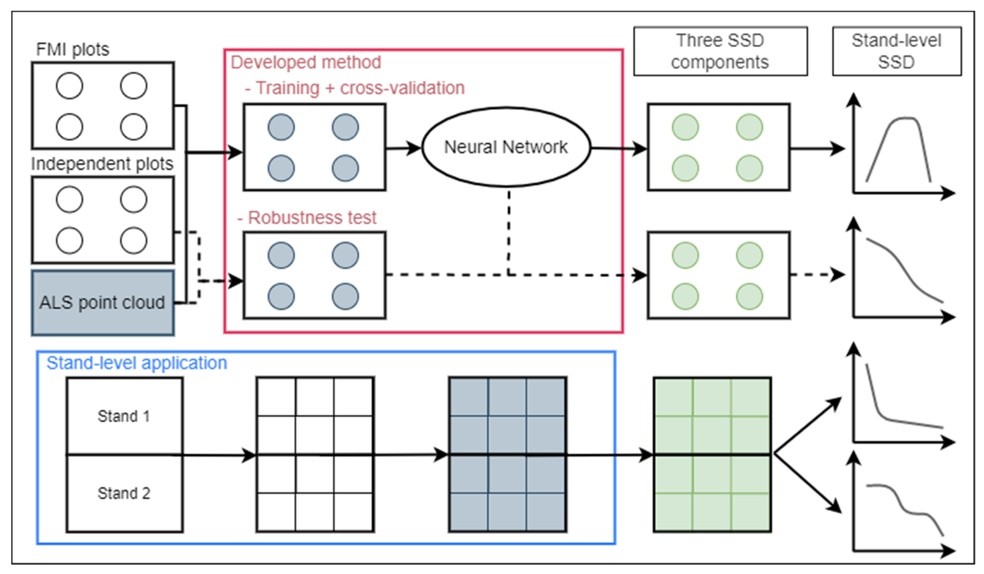
  • To develop a straightforward method for estimating species-specific SSDs using ALS and FMI data for mixed uneven-aged deciduous forests.
  • To use a hybrid approach in which predictions were made at the segment level (i.e., tree crowns were slightly over-segmented, a tree crown could correspond to one or several segments), but thereafter aggregated at stand level.
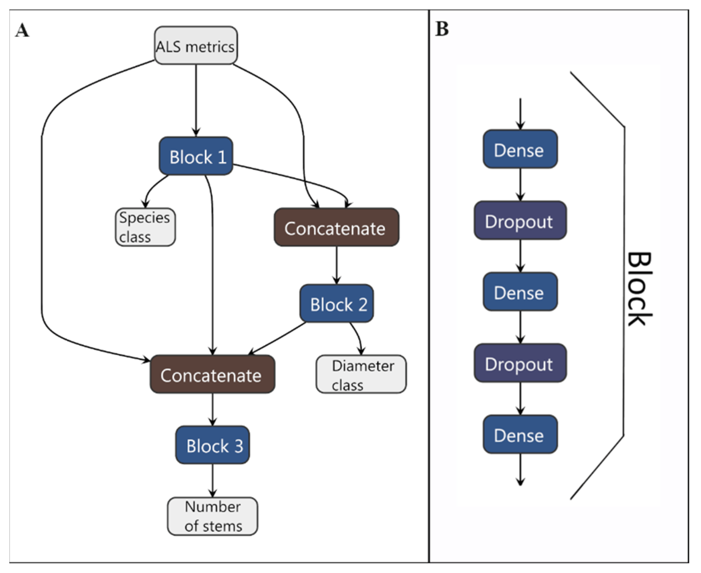
  • To use the potential and versatility of NNs to simultaneously predict the three components required to compute species-specific SSDs: species, circumference class, and number of stems.

2. Materials and Methods
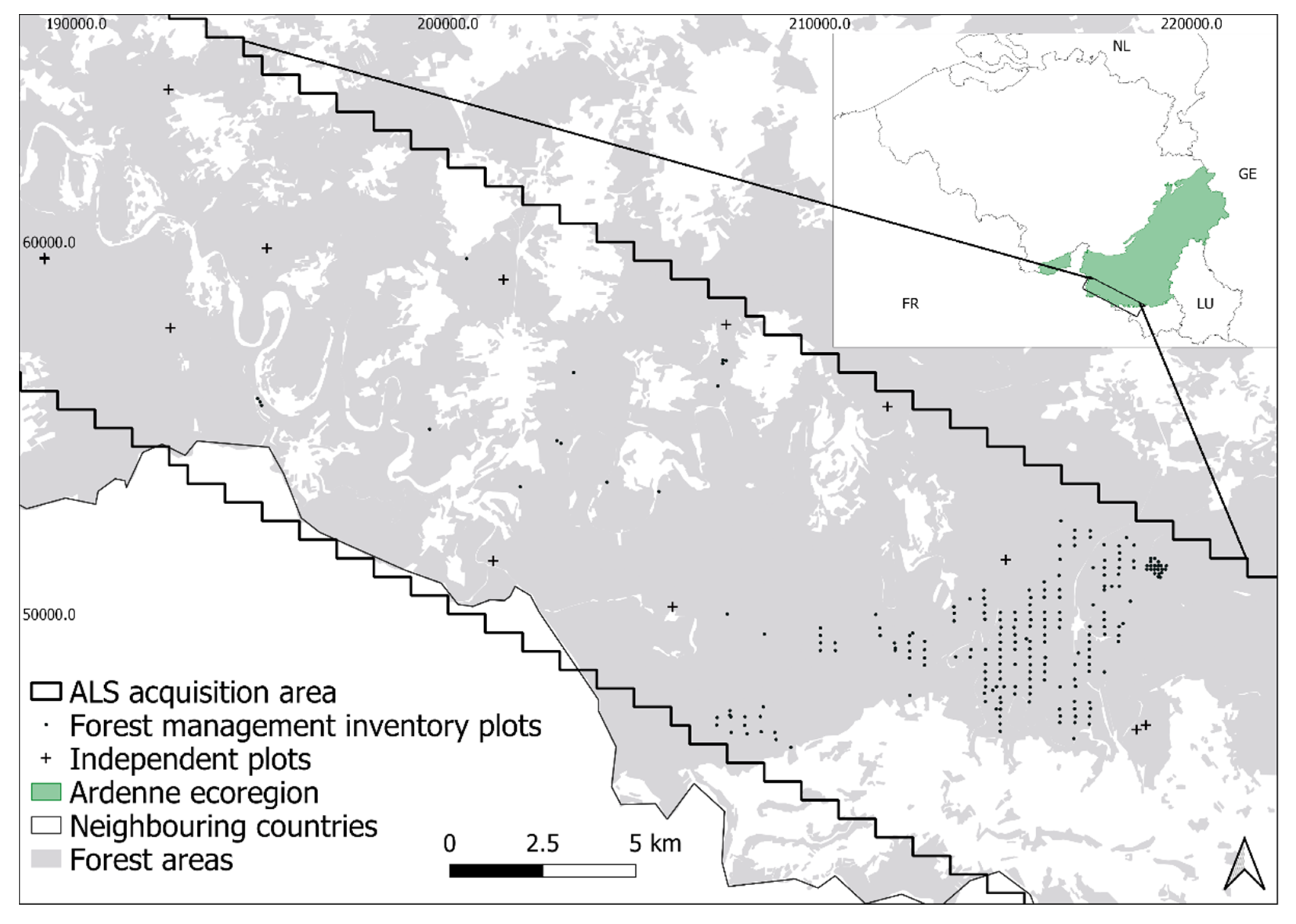
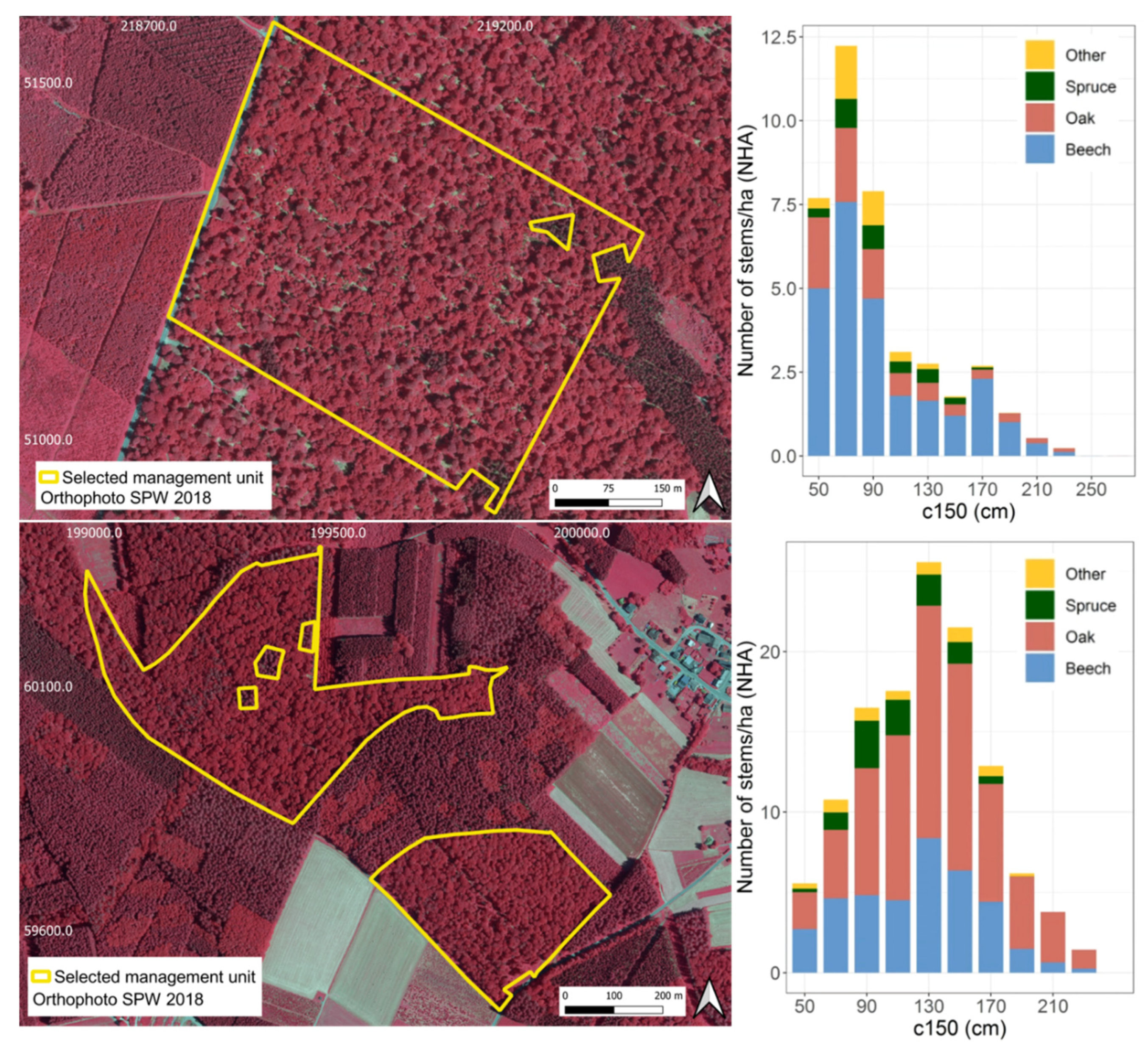
2.1. Study Area

The study area was a mixed uneven-aged deciduous forest of 22,000 ha situated in the Ardenne ecoregion of Wallonia (southern Belgium) (Figure 1). The area’s elevation ranged from 180–432 m and its slope varied from 0–86°. According to the Walloon Regional Forest Inventory [51], oak (Quercus robur L. and Quercus petraea (Mattuschka) Liebl.) represented 44% of the total basal area, followed by beech (Fagus sylvatica L.) with 36%, birch (Betula spp.) with 7%, Norway spruce (Picea abies (L.) H. Karst. subsp. abies) with 3%, and sycamore maple (Acer pseudoplatanus L.) with <2%. This dominant oak–beech mixture is typical of deciduous forests in the ecoregion [51] as a result of past centuries’ forest management favoring oak for its socio-economic value [52].

2.2. Forest Management Inventory Plots

In total, 178 FMI plots were selected within the ALS acquisition area and set up between May 2017 and April 2019 on systematic grids (400 × 200 m for 157 plots, and 100 × 100 m for the other 21) (Figure 1). For each plot, the center was positioned with high precision (x-y error < 1 m) with an Emlid Reach RS+ GPS (Emlid, https://emlid.com/, accessed on 8 February 2022). Plot radius was variable according to stem density in the field but was set to include at least 15 trees, with a maximum value of 18 m (1018 m2 at most). In Wallonia, circumference at 1.5 m height (c150) is traditionally used as a tree-size measurement. c150, species, distance and bearing from plot center were collected for all trees with c150 ≥ 40 cm, the inventory threshold traditionally used in Wallonia (Table 1).

2.3. Independent Plots

A robustness test was implemented using 13 independent plots evenly distributed throughout the study area, mainly outside the forest areas in which the FMI plots were located (Figure 1). Plot area ranged from 1591 to 3511 m2, corresponding to a total sampled surface area of 3.13 ha. Plot position and tree data (Table 2) were surveyed between June and August 2020 using the same methods as for FMIs.

2.4. ALS Data

ALS discrete-return data were acquired using a Optech Titan Dual Wavelength sensor (Teledyne) from 6–9 May 2018 under leaf-on conditions. This sensor allows the simultaneous acquisition of point clouds at a wavelength of 1064 (infra-red; C1 channel) and 532 (green; C2 channel) nm (Table 3). The mean aircraft flight altitude was 684 m above sea level.
ALS data were preprocessed. The point cloud was classified to identify ground hits. Outlier points (i.e., points that were too high above forest canopy) were filtered using statistical methods in the PDAL toolbox [53]. The “mean_k” and “multiplier” parameters were set to 12 and 3, respectively (defined after preliminary tests), and the filtered point cloud was normalized. The CHM was built from the normalized point cloud using the pit-free method [54] of the lidR package [55] with a spatial resolution of 0.5 m. ALS intensity was range-calibrated following [56].

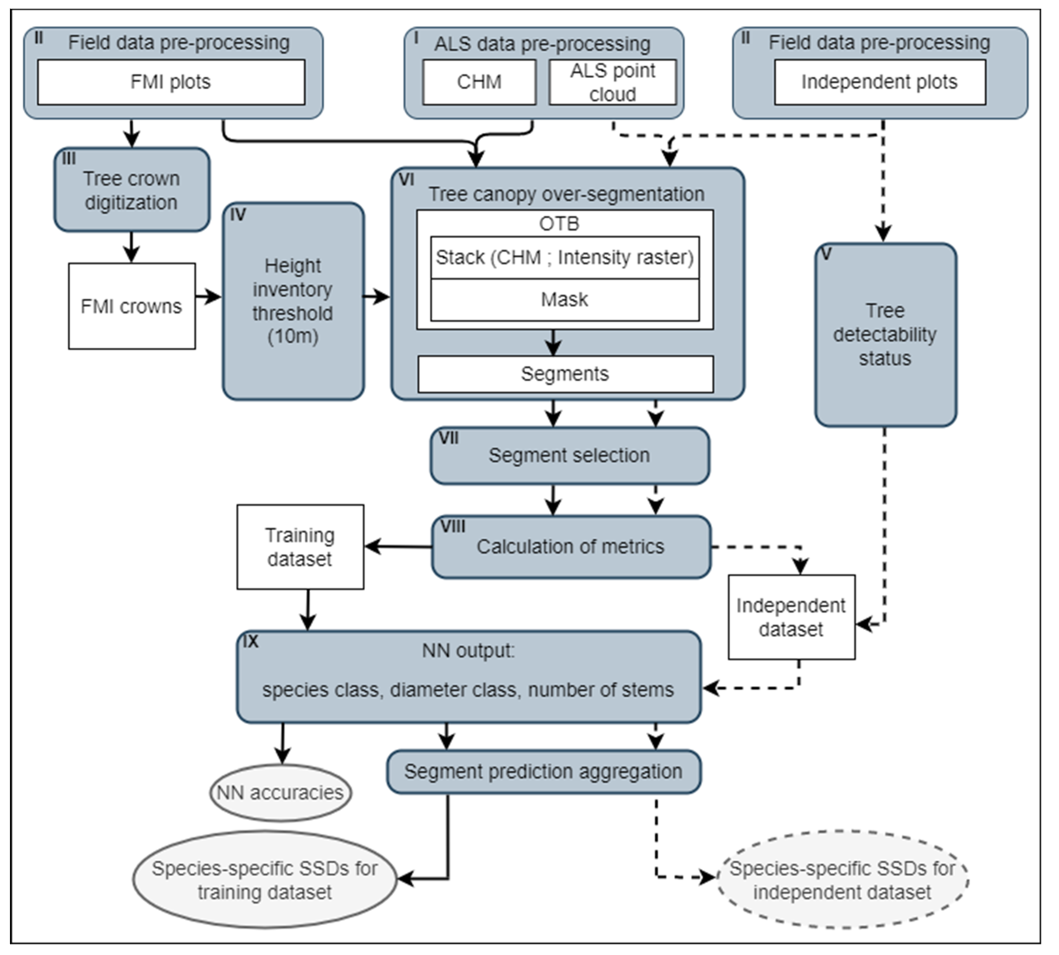
2.5. Overall Approach and Method Overview

Figure 2 illustrates the overall approach of the proposed method designed to use traditional FMIs and ALS data. FMI plots were used to develop the method and train a NN to predict the three components (species, circumference class, and number of stems) at segment level needed to predict the species-specific SSD at stand level. A robustness test was implemented using independent plots located throughout the study area. To demonstrate the method’s application in forest management (stand level application), it was implemented on a regular mesh throughout the study area, with cell predictions subsequently aggregated at stand level.
Figure 3 presents the developed method. Field plots (FMIs and independent) and ALS data were pre-processed, and a canopy height model (CHM) was generated (Figure 3I,II). To avoid tree detection errors, the tree canopy was over-segmented, such that a tree crown could contain one or several segments (Figure 3VI). The segmentation was implemented by considering the height inventory threshold (Figure 3IV). Visible tree crowns in the FMI dataset were digitized by visual interpretation on the CHM (Figure 3III), then used to make the link between segments and FMI data and assign the species, circumference class, and number of stems to each segment (Figure 3VII). The ALS 3D point cloud was used to compute metrics for each segment to create a training dataset (Figure 3VIII). The tree detectability status (Figure 3V) was assessed to maximize the link between field data and remote sensing data. A custom NN was created to simultaneously predict the species class, circumference class, and number of stems at segment level (Figure 3IX). Following NN training, its accuracy was assessed for the three components separately at segment level to evaluate its prediction ability. The three predicted components were then combined to estimate species-specific SSDs at stand level. The NN accuracies were also tested using cross validation. Finally, the fully independent plots were used to set up a robustness test.
The method was developed by considering four species classes (Oak, Beech, Spruce, and Other). All treatments were carried out in R [57] or controlled by R using command lines. LiDAR data processing was performed with the lidR (3.0.4 version) package [55]. Most GIS operations were implemented using the sf [58] and raster [59] R packages.

2.6. Field Data Pre-Processing

Both FMI and independent plot data were pre-processed (Figure 3II). Owing to positioning errors of plot centers, the alignment between the remote sensing and field data was locally deficient. Consequently, plot centers for each dataset were relocated if necessary by photo-interpretation of tree crown position in the CHM. Owing to the time gap between ALS data acquisition and field inventories (≤2 growing seasons), c150 data were corrected using Equation (1) in [60] according to species.

2.7. FMI Crown Digitalization

Tree crowns were manually digitized using the CHM to establish a link between canopy segments and individual trees in the FMI plots in order to (1) construct a training dataset (one tree crown could contain one or several segments, see Canopy segmentation and segment selection step below), and (2) to build models linking tree height and c150 (Figure 3III). These digitized crowns corresponded to trees whose crown boundaries were totally visible and clearly distinguishable on the CHM (no spectral image was available). ALS tree height was calculated as the 98th percentile of CHM pixels inside digitized polygons [61]. This dataset, including only trees visible from the sky, was called “FMI crowns”.

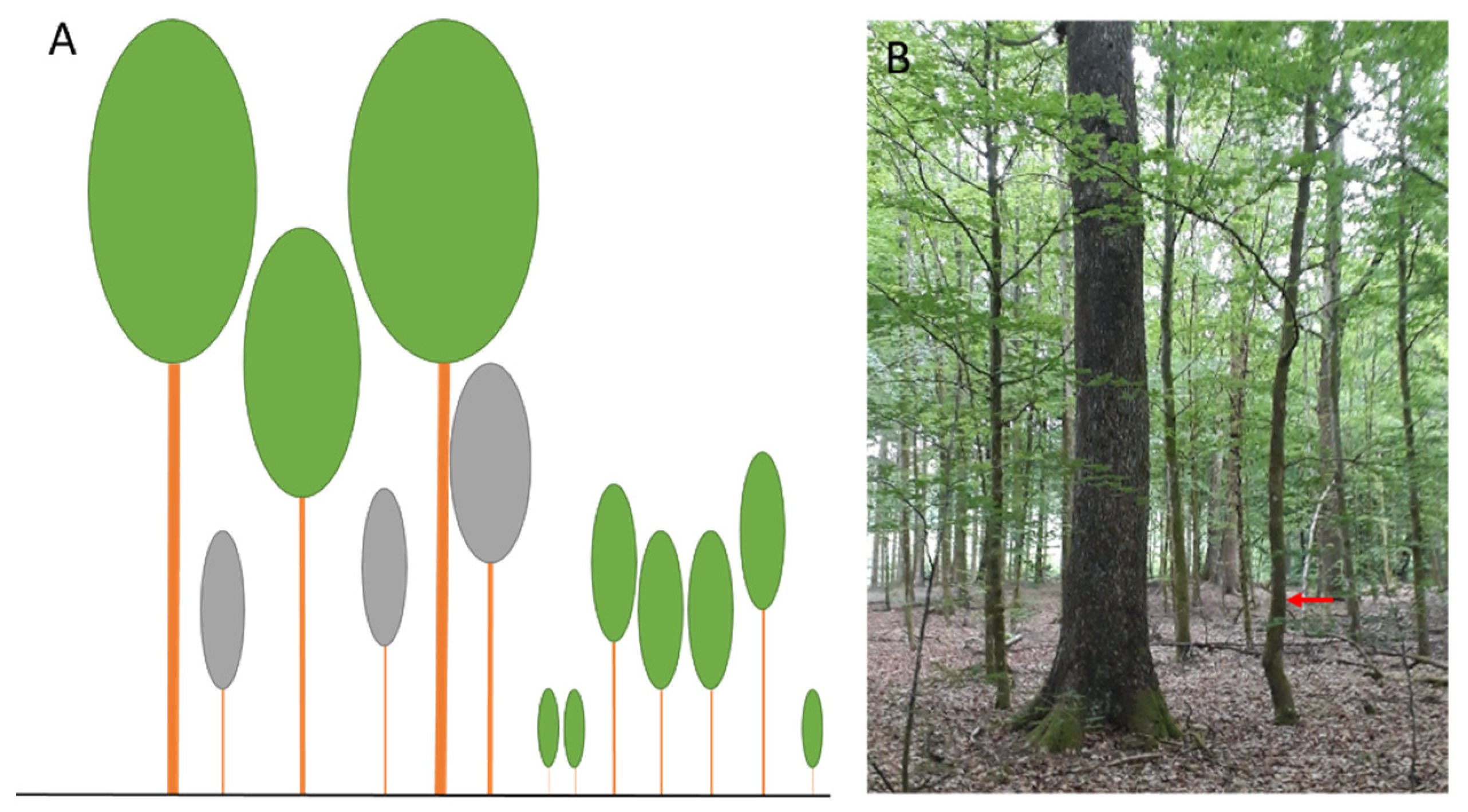
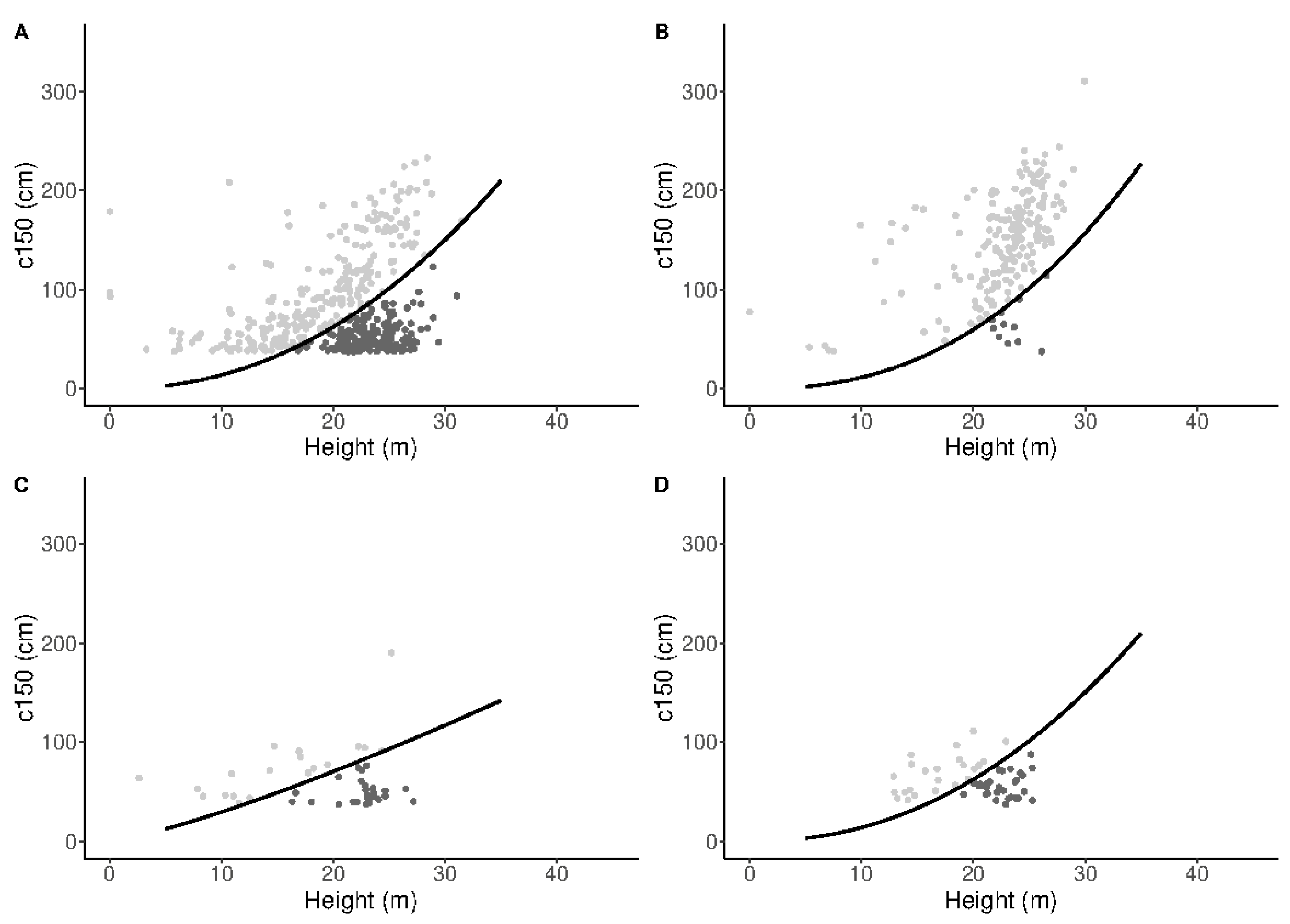
2.8. Tree Detectability Status Assessment

ALS covers the whole forest canopy, composed of (co-)dominant trees and overtopped trees. Overtopped trees correspond to trees with a crown located in lower layer of the canopy. Within dense complex forest stands, overtopped trees are barely visible and less easily detectable, even using ALS data [47,62]. The tree detectability status (Figure 3V) was used to identify the dominated and non-visible trees through ALS data (Figure 4) for the independent dataset.
Tree detectability status was evaluated by comparing the tree c150 with the potential minimum c150 for the observed canopy height (ALS) at the tree position. To predict the potential minimum c150 as a function of ALS canopy height, a model was fitted using FMI crown data (FMI crowns correspond to trees visible from the sky, digitalized on CHM). The FMI crown dataset was used to fit a circumference model on smallest c150 per 2 m height class (Figure 5) for each species class. Trees within independent plots whose c150 was lower than the predicted potential minimum c150 were considered as undetectable trees (overtopped) and excluded from the independent dataset.

2.9. Canopy Segmentation and Segment Selection

We segmented the forest canopy in both FMI and independent plots into objects delimiting whole or partial tree crowns, slightly over-segmenting tree crowns to better delimit crown edges and avoid omission errors (Figure 3VI).
The segmentation was done by plot (+30 m buffer to avoid edge effects) for areas of the FMI and independent plots using the mean-shift algorithm of the Orfeo toolbox [63]. A raster containing two bands (spatial resolution 0.50 cm) derived from ALS data was used as the image to segment: the CHM (rescaled between 0–1000) and an intensity raster (including both intensities; rescaled between 0–2000). The spatial radius, range radius, and minimum region size were set to 20, 40, and 15, respectively. Parameter values were fixed after a sensitivity analysis. The two band raster was masked before segmentation. Only areas with CHM ≥ 10 m (height threshold based on field observations) and CHM slope < 75° (to suppress low branches at canopy edges) were considered.
Training and independent datasets were then created by selecting segments crossing FMI crowns and borders of independent plots, respectively (Figure 3VII). The training dataset was used to train the NN and test the species-specific SSD estimations. The independent dataset was used to test the method’s robustness.
Like the edge-tree correction method developed for ABA in [64], a segment was selected if its local maximum (LM) was located inside the FMI crowns or plot. LMs were generated from the CHM considering the pixel with the maximum height value inside each segment. For each segment of the training dataset, the species class and c150 of the corresponding FMI crowns were attributed to the segment. As mentioned above, the forest canopy was over-segmented to avoid omission errors, so the number of stems for the considered segment was calculated as the ratio of the segment area to the area of the corresponding FMI crown. The average number of stems per segment was 0.19.

2.10. Calculation of Metrics

Following previous research [26,32,33,35,43,44], 46 ALS features were calculated for each segment (Figure 3VIII). Height metrics were calculated considering points above 2 m. Intensity metrics were calculated considering points above the 85th height percentile inside segments for both channels (C1 and C2). Several vegetation indices combining the mean intensity of each channel were also calculated for each segment. These metrics are described in the Appendix A (Table A1).

2.11. Neural Network Implementation

Species-specific SSDs were derived from three successive and dependent components: species class, circumference class, and number of stems. The relationship between ALS and field variables strongly varies depending on the species, and for a given species within a given area, circumference is one of the most important explanatory variables for estimating the number of stems [33,60]. Errors in these estimations thus accumulate and exacerbate one other. In the proposed method, a NN with a custom architecture was implemented to simultaneously predict the three components (Figure 3IX). The c150 was converted into 20 cm wide circumference classes. The training dataset consisted of tabular data containing the three components for each segment and the ALS metrics. The NN architecture allowed consideration of the between-component retroactive effects during training, thus optimizing the learning and maximizing the precision of the three component estimations. NN data preparation, architecture, and training were operated in R using the keras R package [65] with TensorFlow as the backend.
NN implementation required input and output data preparation. The input numerical variables (i.e., ALS metrics) were normalized to have a mean of 0 and a standard deviation of 1. Concerning output data, the two categorical variables (species class and circumference class) were converted into binary variables (dummy). The conversion method was different for species class (as the nominal variable) and circumference class (as the ordinal variable) [66]. For instance, a categorical variable of five classes with a value of 3 equals 0–0-1–0-0 if nominal and 1–1-0–0-0 if ordinal [67,68]. No modification was made to the number of stems. Species class was converted into four binary variables and circumference class into twelve (Table 4).
A specific architecture composed of three blocks (Figure 6) was created to simultaneously predict the three components required to compute the species-specific SSDs: species class (block 1), circumference class (block 2), and number of stems (block 3). These three blocks had the same architecture but independent weights. Each block was composed of three successive dense layers (Figure 6). The first two comprised 32 hidden nodes followed by the ‘hyperbolic tangent’ activation function [69] and a dropout of 25% [70]. The number of hidden nodes and dropout percentage were defined to avoid over-fitting issues. The third dense layer was only used for data reconstruction followed by one specific activation function (Table 4). The total model trainable weight parameters numbered 8881.
For NN training, the Adam optimizer was used with a learning rate of 0.005. The overall loss was computed by summing the three losses (Table 4). The training was stopped when the overall loss reached a plateau [71]. During training, as the input data were not fully balanced, losses of species classes and circumference classes were weighted jointly. These weights were inversely proportional to the segment occurrence, forcing the model to pay more attention to the less frequent classes. In combination with the small number of hidden nodes and the dropouts, this ensured high NN robustness and generalization ability.

2.12. Neural Network Accuracy

The NN accuracy was assessed at the end of the training stage for the three components separately using appropriate accuracy indices (Table 4). This assessment was made on the entire training dataset considering predictions at segment level. Categorical variables (species class and circumference class) were assessed through confusion matrices comparing training and prediction classes. The number of stems was assessed considering R2 (Table 4), RMSE, and bias.
The three components predicted at the segment level were aggregated to predict the species-specific SSDs at stand level (all plots considered), considering the entire training dataset. The number of stems per hectare by circumference class and by species was calculated and compared with the field data. To evaluate the species-specific SSD estimations, the Reynolds index (Equation (1)) [72] and Packalén index (Equation (2)) [16] were calculated overall and by species; these indices are commonly used to assess the accuracy of SSD estimation [32,35,36,37,39,41]:
Reynolds   Index = c = 1 m 100 × | f c f ^ c N | ,
Packalén   Index = c = 1 m 0.5 × | f c N f ^ c N ^ | ,
where c is the circumference class from 1 to m, f c is the observed stem density in the circumference class c, f ^ c is the predicted stem density in the circumference class c, N is the observed total stem density, and N ^ is the predicted total stem density. Stem density was calculated per hectare considering all plots. A value of 0 for these indices corresponds to a perfect estimation. The Reynolds index could range from 0 to an infinite value while the Packalén index is bounded between 0 and 1.
The NN was also evaluated using a simple cross-validation using the segments of 80% of the randomly selected plots (training data for the cross-validation). The model was then tested on the segments contained in the 20% remaining plots (validation data for the cross-validation). One hundred repetitions were performed; in each, the NN accuracy of the three components and species-specific SSD estimations were evaluated considering the validation dataset. The species class and circumference class were assessed using the overall accuracy and the number of stems was assessed by R2. Based on SSD estimation, the residual stem density by circumference class and species were calculated, and the Reynolds and Packalen indices were also evaluated for each repetition.

2.13. Robustness Test

The proposed method was also tested on the independent dataset (Figure 1 and Figure 3), which was evenly distributed over the study area and mainly outside the FMI plot location. This allowed an assessment of the method’s quality and robustness over the entire study area, including more variability in structure and composition (species proportions). Species class, circumference class, and number of stems were predicted for each segment of the independent dataset. Segment predictions were aggregated to estimate the species-specific SSDs at stand level.

3. Results

3.1. Neural Network Accuracy

The NN predicted the species class with a categorical overall accuracy of 0.92. The confusion matrix is presented in Table 5. The user and producer accuracies ranged from 0.85–0.97 and 0.89–0.99, respectively, both with the highest value for spruce. Most confusion took place between deciduous species, especially between oak and beech. The circumference class (c150) was predicted with an ordinal overall accuracy of 0.36. The corresponding confusion matrix is presented in Table 6. The user and producer accuracies ranged from 0.11–0.92 and 0.06–0.84, respectively, with confusion between circumference classes usually occurring between close classes. This effect seemed to be accentuated for the central classes (110–210). The number of stems was predicted with an R2 value of 0.90, a RMSE of 0.09, and a bias of 0.00.
The predictions of the three components of each segment were combined to compute the species-specific SSDs per hectare at stand level for the whole training dataset (Figure 7). The values of the overall Reynolds and Packalén indices were 21.15 and 0.10, respectively. The total number of stems per hectare inventoried and estimated were 224 and 219, respectively. These accuracies varied according to species class (Table 7).
The cross-validation results for the accuracy of the three components were lower than for the global adjustment on the whole training dataset (Figure 8). The residual standard deviations of the stem density by circumference class and species are presented in Figure 7. The Reynolds and Packalén index values were variable depending on the considered species class (Figure 9). On average, these index values were lower when all species were considered, as well as for beech and spruce (Figure 9).

3.2. Robustness Test Using the Independent Dataset

The method was also tested on the independent dataset (Figure 10). The values of the overall Reynolds and Packalén indices were 53.98 and 0.18, respectively, and the total number of stems per hectare inventoried and predicted were 151.5 and 190.7, respectively. These accuracies also varied according to species class (Table 8), and were lower than the global NN accuracies (Table 7). The results of the robustness test were higher for the two main species (oak and beech), which corresponded to 94% of the total basal area of the independent dataset (Table 8). For beech, a certain shift can be observed between small (50–70) and intermediate (90–170) circumference classes (Figure 10).
As an example, the developed method was used to estimate species-specific SSDs at stand level for two management units located in the study area (Figure 11).

4. Discussion

Our proposed method allowed precise stand-level prediction of species-specific SSDs in a mixed uneven-aged deciduous forest of 22,000 ha. A specific NN was implemented to simultaneously predict the three components required to compute species-specific SSDs (species class, circumference class, and number of stems). Low Reynolds and Packalén index values for the training dataset (Table 7) showed the ability of the NN model to predict the species-specific SSDs for the training dataset. The cross-validation showed comparable accuracy values. The results of the robustness test also had high accuracy values, both overall and for the two main species (beech and oak) (Table 8), even if they were globally a little lower than the results of the training phase. This seemed consistent since the robustness test was performed with completely independent data located outside the FMI plot locations (training area).
It was difficult to rigorously compare our results with those of other similar studies due to methodological differences. For example, studied forests varied significantly, field inventory data were mostly different, and remote sensing data had various properties. However, comparisons can be made of the methods themselves, considering their particularities, strengths, weaknesses, and their ability to meet scientific and management needs. The SSD was estimated from the three predicted components at segment level using a single NN. The proposed method does not require successive allometric relations or DBH models as in other studies [33,35,38,39]. Nor does it require choosing the form of any relationship among variables as in parametric approaches [32]. It did not require prior knowledge of the structure or any need to predefine other variables. Similar to [32], our method is highly versatile and can potentially be adapted to any type of forest. Some studies made overall predictions but without distinguishing tree species [32,33,35,41]; the last study focused on homogeneous coniferous stands dominated by spruce but with a wide range of complex terrains. Ref [39] predicted broadleaf proportion considering that stem diameters were equidistant quantiles of a Weibull distribution. Ref [40] produced species-specific predictions but used a preliminary plot stratification by main species during the sampling design. Similar to [21], who made species-specific predictions considering three species classes (pine, spruce, and deciduous) using ALS and aerial imageries, our method was able to make precise species-specific predictions from bi-spectral ALS metrics. However, the digitization of tree crowns to create the training dataset was required and could be seen as a limitation. However, due to the high complexity of the targeted forest’s structure and species composition, the segmentation quality achievable using traditional tools [73,74,75] would not be sufficient to avoid this step.
Concerning species discrimination, Ref.[43] used three-wavelength ALS data to discriminate up to 10 species and showed that confusion appeared less frequently between coniferous and broadleaved species. This was confirmed by our results, in which the spruce class was better discriminated than the other three; as in [76], the main confusion occurred between deciduous species. The Other class, which included different deciduous species, had the lowest accuracy as that of the least well-represented classes is often lower and more difficult to interpret [76].
A robustness test was performed to evaluate the results’ quality on a completely independent data set. This confirmed that the method worked quite well for the main species, especially oak, while a certain shift was observed for beech between the small and intermediate circumference classes. In fact, the forest considered in the study area was particularly complex and heterogeneous in both structure and composition. It is possible that the relationship between ALS metrics and the three components differed slightly in space owing to variations in silvicultural practices or growing conditions. NNs are known to generalize and are capable of learning main patterns from partial data if training data are sufficiently representative for the targeted area. A larger dataset for the less-well-represented species and circumference classes could improve the results. Additional data on soil properties, forest productivity, or other variables could also be included.
The NN with a custom architecture allowed the simultaneous prediction of the three components required to estimate species-specific SSD. Furthermore, the retroactive effect of the errors of these components (i.e., the adjustment of the three components within the neural network is not done independently) was taken into account during the adjustment, which improved the overall accuracy.
Our proposed method optimizes the link between field data and remote sensing data. The tree detectability through ALS data was assessed for trees of the independent plots to improve SSDs evaluation. Such procedures are not mandatory for less complex forests that are single-species or even-aged [33]. Correcting estimates according to tree detectability status may appear to be a limitation. This is not an issue for silvicultural practices because these trees usually correspond to small trees (c150 < 90 cm) with a low future value. These trees correspond to 9.40% of the total basal area per hectare. In contrast, the study area was mainly a productive forest where established regeneration is rapidly uncovered by managers to meet sapling light requirements. In addition, the forest structure also induced the development of sapling groups. Enhanced detection of understory trees could be achieved using a higher-density point cloud (≥170 pt/m2 to detect trees in the third canopy layer) [77]. The multidimensional deep learning [78,79] or the 3D point cloud segmentation [47,80] could potentially improve understory tree detection to predict species-specific SSD. Leaf-off ALS data could also be preferable for detecting understory trees [81].
Our proposed method is versatile and should be adapted to work on any forests, thus having great potential for improving forest management by allowing the prediction of species-specific SSDs at stand level. It requires only traditional FMI and bi-spectral ALS data, canopy segmentation, calculation of metrics, and NN training. FMIs are frequently conducted in most managed forests and ALS data acquisition is rapidly becoming more accessible and will be more frequently used in the near future. Nevertheless, the required manual digitalization of tree crowns to create a training dataset is a barrier to adoption. Further work should focus mainly on three points: (1) implementing the method in other types of forest, (2) generalizing the procedure for linking field data and remote sensing data, and (3) determining the optimal number of plots and digitized crowns (by species and circumference class) to capture the variability of the area of interest [82,83].

5. Conclusions

Our proposed method allowed a precise stand-level estimate of species-specific SSDs in a mixed uneven-aged deciduous forest of 22,000 ha using ALS and FMI data. The method was not dependent on the tree detection rate. A specific NN (customized architecture) was used to simultaneously predict the three required components (species class, circumference class, and number of stems). Although the method should be tested with other forests (different structures and tree species compositions), the results are promising for forest management.

Author Contributions

Conceptualization, L.L., N.L. and P.L.; methodology, L.L., N.L. and P.L.; software, L.L. and N.L.; validation, L.L.; formal analysis, L.L.; resources, L.L.; data curation, L.L.; writing—original draft preparation, L.L. and N.L.; writing—review and editing, N.L., P.L. and C.B.; visualization, L.L., N.L. and P.L.; supervision, P.L.; project administration, L.L. and P.L.; funding acquisition, P.L. All authors have read and agreed to the published version of the manuscript.

Funding

This research was funded by Interreg Grande Region-Regiowood II, grant number 019–2-03–032, and Walloon Region Forest Administration through the CARTOFOR project, which is part of a five-year forest research and training plan (2019–2024).

Institutional Review Board Statement

Not applicable.

Informed Consent Statement

Not applicable.

Data Availability Statement

The datasets used in this research are available on demand from the corresponding author.

Acknowledgments

The authors thank the Direction des Cours d’eau non navigables—Service Public de Wallonie (SPW) for ALS data acquisition and sharing; Borremans A., Delinte T., Geerts C., Lemaigre B., and Monseur A. for field data collection; and the Département de la Nature et des Forêts—SPW, in particular the Bièvre, Bouillon, Florenville, and Neufchateau Sections, for their collaboration.

Conflicts of Interest

The authors declare no conflict of interest. The funders had no role in the design of the study; in the collection, analyses, or interpretation of data; in the writing of the manuscript, or in the decision to publish the results.

Appendix A

Table A1. ALS metrics calculated for each segment. The name of each metric is indicated and followed by a description. Intensity metrics were calculated for both channels (C1 and C2).
Geometric MetricsDescription
area_m2Segment area (m2)
Height metricsDescription
accAverage height increase from 2014–2018 (m/year)
sd_CHMStandard deviation of CHM pixels (m)
cv_CHMCoefficient of variation of CHM pixels
sd_hStandard deviation (m) of point heights
cv_hCoefficient of variation of point heights
kurt_hKurtosis of point heights
skew_hSkewness of point heights
cv_ladCoefficient of variation of the leaf area density
entr_hEntropy of point heights
ah_ratioRatio of segment area to 98th percentile of CHM pixels
riRumple index of point heights
mn_slope_hAverage slope calculated between the highest point and all other points
sd_slope_hStandard deviation of slope calculated between the highest point and all other points
mn_slope_h_frAverage slope calculated between the highest first return point and all other first return points
sd_slope_h_frStandard deviation of slope calculated between the highest first return point and all other first return points
Intensity metricsDescription
max_i_c1Maximum of point intensity for the C1 channel
mean_i_c1Mean of point intensity for the C1 channel
sd_i_c1Standard deviation of point intensity for the C1 channel
kurt_i_c1Kurtosis of point intensity for the C1 channel
skew_i_c1Skewness of point intensity for the C1 channel
cv_i_c1Coefficient of variation of point intensity for the C1 channel
entr_i_c1Entropy of point intensity for the C1 channel
max_i_fr_c1Mean of point intensity for the C1 channel; first returns only
mean_i_fr_c1Mean of point intensity for the C1 channel; first returns only
sd_i_fr_c1Standard deviation of point intensity for the C1 channel; first returns only
cv_i_fr_c1Coefficient of variation of point intensity for the C1 channel; first returns only
kurt_i_fr_c1Kurtosis of point intensity for the C1 channel; first returns only
skew_i_fr_c1Skewness of point intensity for the C1 channel; first returns only
entr_i_fr_c1Entropy of point intensity for the C1 channel; first returns only
max_i_c2Maximum of point intensity for the C2 channel
mean_i_c2Mean of point intensity for the C2 channel
sd_i_c2Standard deviation of point intensity for the C2 channel
kurt_i_c2Kurtosis of point intensity for the C2 channel
skew_i_c2Skewness of point intensity for the C2 channel
cv_i_c2Coefficient of variation of point intensity for the C2 channel
entr_i_c2Entropy of point intensity for the C2 channel
max_i_fr_c2Mean of point intensity for the C2 channel; first returns only
mean_i_fr_c2Mean of point intensity for the C2 channel; first returns only
sd_i_fr_c2Standard deviation of point intensity for the C2 channel; first returns only
cv_i_fr_c2Coefficient of variation of point intensity for the C2 channel; first returns only
kurt_i_fr_c2Kurtosis of point intensity for the C2 channel; first returns only
skew_i_fr_c2Skewness of point intensity for the C2 channel; first returns only
entr_i_fr_c2Entropy of point intensity for the C2 channel; first returns only
Vegetation indexDescription
ndgi_mm_fGreen normalized difference vegetation index
(mean_i_C1 − mean_i_C2)/(mean_i_C1 + mean_i_C2)
r_topo_bathyChannel ratio
mean_I_C1/mean_I_C2

References

  1. FAO. Global Forest Ressources Assessment 2020—Key Findings; FAO: Rome, Italy, 2020. [Google Scholar]
  2. O’Hara, K.L.; Gersonde, R.F. Stocking control concepts in uneven-aged silviculture. Forestry 2004, 77, 131–143. [Google Scholar] [CrossRef]
  3. Boncina, A.; Diaci, J.; Cencic, L. Comparison of the two main types of selection forests in Slovenia: Distribution, site conditions, stand structure, regeneration and management. Forestry 2002, 75, 365–373. [Google Scholar] [CrossRef] [Green Version]
  4. Duchateau, E.; Schneider, R.; Tremblay, S.; Dupont-Leduc, L. Density and diameter distributions of saplings in naturally regenerated and planted coniferous stands in Québec after various approaches of commercial thinning. Ann. For. Sci. 2020, 77, 38. [Google Scholar] [CrossRef]
  5. Rubin, B.D.; Manion, P.D.; Faber-Langendoen, D. Diameter distributions and structural sustainability in forests. For. Ecol. Manag. 2006, 222, 427–438. [Google Scholar] [CrossRef]
  6. Cameron, A.; Prentice, L. Determining the sustainable irregular condition: An analysis of an irregular mixed-species selection stand in Scotland based on recurrent inventories at 6-year intervals over 24 years. Forestry 2016, 89, 208–214. [Google Scholar] [CrossRef] [Green Version]
  7. Næsset, E. Area-Based inventory in norway—From innovation to an operational reality. In Forestry Applications of Airborne Laser Scanning; Springer: Berlin/Heidelberg, Germany, 2014; pp. 215–240. [Google Scholar] [CrossRef]
  8. Kangas, A.; Astrup, R.; Breidenbch, J.; Fridman, J.; Gobakken, T.; Korhonen, K.T.; Maltamo, M.; Nilsson, M.; Nord-Larsen, T.; Naesset, E.; et al. Remote sensing and forest inventories in Nordic countries—Roadmap for the future. Scand. J. For. Res. 2018, 33, 397–412. [Google Scholar] [CrossRef] [Green Version]
  9. Maltamo, M.; Packalen, P.; Kangas, A. From comprehensive field inventories to remotely sensed wall-to-wall stand attribute data—A brief history of management inventories in the nordic countries. Can. J. For. Res. 2020, 51, 257–266. [Google Scholar] [CrossRef]
  10. Rondeux, J. La Mesure des Arbres et des Peuplements Forestiers, 3rd ed.; Les Presses Agronomiques de Gembloux: Gembloux, Belgium, 2021. [Google Scholar]
  11. Lei, X.D.; Tang, M.P.; Lu, Y.C.; Hong, L.X.; Tian, D.L. Forest inventory in China: Status and challenges. Int. For. Rev. 2009, 11, 52–63. [Google Scholar] [CrossRef]
  12. Rahlf, J.; Hauglin, M.; Astrup, R.; Breidenbach, J. Timber volume estimation based on airborne laser scanning—Comparing the use of national forest inventory and forest management inventory data. Ann. For. Sci. 2021, 78, 49. [Google Scholar] [CrossRef]
  13. Hoover, C.M.; Bush, R.; Palmer, M.; Treasure, E. Using forest inventory and analysis data to support national forest management: Regional case studies. J. For. 2020, 118, 313–323. [Google Scholar] [CrossRef]
  14. Vega, C.; Renaud, J.-P.; Sagar, A.; Bouriaud, O. A new small area estimation algorithm to balance between statistical precision and scale. Int. J. Appl. Earth Obs. Geoinf. 2021, 97, 102303. [Google Scholar] [CrossRef]
  15. Scott, C.T.; Gove, J.H. Forest inventory. Encycl. Environ. 2002, 2, 814–820. [Google Scholar]
  16. Packalén, P.; Maltamo, M. Estimation of species-specific diameter distributions using airborne laser scanning and aerial photographs. Can. J. For. Res. 2008, 38, 1750–1760. [Google Scholar] [CrossRef]
  17. Maltamo, M.; Næsset, E.; Bollandsås, O.M.; Gobakken, T.; Packalén, P. Non-parametric prediction of diameter distributions using airborne laser scanner data. Scand. J. For. Res. 2009, 24, 541–553. [Google Scholar] [CrossRef]
  18. Peuhkurinen, J.; Maltamo, M.; Malinen, J. Estimating species-specific diameter distributions and saw log recoveries of boreal forests from airborne laser scanning data and aerial photographs: A distribution-based approach. Silva Fenn. 2008, 42, 625–641. [Google Scholar] [CrossRef] [Green Version]
  19. Peuhkurinen, J.; Tokola, T.; Plevak, K.; Sirparanta, S.; Kedrov, A.; Pyankov, S. Predicting tree diameter distributions from airborne laser scanning, SPOT 5 satellite, and field sample data in the Perm Region, Russia. Forests 2018, 9, 639. [Google Scholar] [CrossRef] [Green Version]
  20. Strunk, J.L.; Gould, P.J.; Packalen, P.; Poudel, K.P.; Andersen, H.E.; Temesgen, H. An examination of diameter density prediction with k-NN and airborne lidar. Forests 2017, 8, 444. [Google Scholar] [CrossRef] [Green Version]
  21. Räty, J.; Packalen, P.; Maltamo, M. Comparing nearest neighbor configurations in the prediction of species-specific diameter distributions. Ann. For. Sci. 2018, 75, 1–16. [Google Scholar] [CrossRef] [Green Version]
  22. Mauro, F.; Frank, B.; Monleon, V.J.; Temesgen, H.; Ford, K.R. Prediction of diameter distributions and tree-lists in southwestern oregon using lidar and stand-level auxiliary information. Can. J. For. Res. 2019, 49, 775–787. [Google Scholar] [CrossRef]
  23. Maltamo, M.; Mehtätalo, L.; Valbuena, R.; Vauhkonen, J.; Packalen, P. Airborne laser scanning for tree diameter distribution modelling: A comparison of different modelling alternatives in a tropical single-species plantation. Forestry 2017, 91, 121–131. [Google Scholar] [CrossRef]
  24. Arias-Rodil, M.; Diéguez-Aranda, U.; Álvarez-González, J.G.; Pérez-Cruzado, C.; Castedo-Dorado, F.; González-Ferreiro, E. Modeling diameter distributions in radiata pine plantations in Spain with existing countrywide LiDAR data. Ann. For. Sci. 2018, 75, 36. [Google Scholar] [CrossRef] [Green Version]
  25. Cosenza, D.N.; Soares, P.; Guerra-Hernandez, J.; Pereira, L.; Gonzalez-Ferreiro, E.; Castedo-Dorado, F.; Tomé, M. Comparing Johnson’s SB and weibull functions to model the diameter distribution of forest plantations through ALS data. Remote Sens. 2019, 11, 2792. [Google Scholar] [CrossRef] [Green Version]
  26. Zhang, Z.; Cao, L.; Mulverhill, C.; Liu, H.; Pang, Y.; Li, Z. Prediction of diameter distributions with multimodal models using LiDAR data in subtropical planted forests. Forests 2019, 10, 125. [Google Scholar] [CrossRef] [Green Version]
  27. Gobakken, T.; Næsset, E. Estimation of diameter and basal area distributions in coniferous forest by means of airborne laser scanner data. Scand. J. For. Res. 2004, 19, 529–542. [Google Scholar] [CrossRef]
  28. Gorgoso, J.J.; Alvarez Gonzalez, J.G.; Rojo, A.; Grandas-Arias, J.A. Modelling diameter distributions of Betula alba L. stands in northwest Spain with the two-parameter Weibull function. Investig. Agrar. Sist. Recur. For. 2007, 16, 113–123. [Google Scholar] [CrossRef] [Green Version]
  29. Maltamo, M.; Suvanto, A.; Packalén, P. Comparison of basal area and stem frequency diameter distribution modelling using airborne laser scanner data and calibration estimation. For. Ecol. Manag. 2007, 247, 26–34. [Google Scholar] [CrossRef]
  30. Breidenbach, J.; Gläser, C.; Schmidt, M. Estimation of diameter distributions by means of airborne laser scanner data. Can. J. For. Res. 2008, 38, 1611–1620. [Google Scholar] [CrossRef]
  31. Thomas, V.; Oliver, R.D.; Lim, K.; Woods, M. LiDAR and Weibull modeling of diameter and basal area. For. Chron. 2008, 84, 866–875. [Google Scholar] [CrossRef] [Green Version]
  32. Mulverhill, C.; Coops, N.C.; White, J.C.; Tompalski, P.; Marshall, P.L.; Bailey, T. Enhancing the estimation of stem-size distributions for unimodal and bimodal stands in a boreal mixedwood forest with airborne laser scanning data. Forests 2018, 9, 95. [Google Scholar] [CrossRef] [Green Version]
  33. Paris, C.; Bruzzone, L. A growth-model-driven technique for tree stem diameter estimation by using airborne LiDAR data. IEEE Trans. Geosci. Remote Sens. 2018, 57, 76–92. [Google Scholar] [CrossRef]
  34. Malek, S.; Miglietta, F.; Gobakken, T.; Næsset, E.; Gianelle, D.; Dalponte, M. Prediction of stem diameter and biomass at individual tree crown level with advanced machine learning techniques. iForest-Biogeosciences For. 2019, 12, 323–329. [Google Scholar] [CrossRef] [Green Version]
  35. Räty, J.; Packalen, P.; Kotivuori, E.; Maltamo, M. Fusing diameter distributions predicted by an area-based approach and individual-tree detection in coniferous-dominated forests. Can. J. For. Res. 2020, 50, 113–125. [Google Scholar] [CrossRef]
  36. Vauhkonen, J.; Mehtätalo, L. Matching remotely sensed and field-measured tree size distributions. Can. J. For. Res. 2015, 45, 353–363. [Google Scholar] [CrossRef]
  37. Xu, Q.; Hou, Z.; Maltamo, M.; Tokola, T. Calibration of area based diameter distribution with individual tree based diameter estimates using airborne laser scanning. ISPRS J. Photogramm. Remote Sens. 2014, 93, 65–75. [Google Scholar] [CrossRef]
  38. Kansanen, K.; Vauhkonen, J.; Lähivaara, T.; Seppänen, A.; Maltamo, M.; Mehtätalo, L. Estimating forest stand density and structure using Bayesian individual tree detection, stochastic geometry, and distribution matching. ISPRS J. Photogramm. Remote Sens. 2019, 152, 66–78. [Google Scholar] [CrossRef]
  39. Spriggs, R.A.; Coomes, D.A.; Jones, T.A.; Caspersen, J.P.; Vanderwel, M.C. An alternative approach to using LiDAR remote sensing data to predict stem diameter distributions across a temperate forest landscape. Remote Sens. 2017, 9, 944. [Google Scholar] [CrossRef] [Green Version]
  40. Magnussen, S.; Renaud, J.P. Multidimensional scaling of first-return airborne laser echoes for prediction and model-assisted estimation of a distribution of tree stem diameters. Ann. For. Sci. 2016, 73, 1089–1098. [Google Scholar] [CrossRef] [Green Version]
  41. Shang, C.; Treitz, P.; Caspersen, J.; Jones, T. Estimating stem diameter distributions in a management context for a tolerant hardwood forest using ALS height and intensity data. Can. J. Remote Sens. 2017, 43, 79–94. [Google Scholar] [CrossRef]
  42. Ferraz, A.; Saatchi, S.S.; Longo, M.; Clark, D.B. Tropical tree size–frequency distributions from airborne lidar. Ecol. Appl. 2020, 30, 2154. [Google Scholar] [CrossRef]
  43. Budei, B.C.; St-Onge, B.; Hopkinson, C.; Audet, F.A. Identifying the genus or species of individual trees using a three-wavelength airborne lidar system. Remote Sens. Environ. 2018, 204, 632–647. [Google Scholar] [CrossRef]
  44. Dalponte, M.; Ene, L.T.; Gobakken, T.; Næsset, E.; Gianelle, D. Predicting selected forest stand characteristics with multispectral ALS data. Remote Sens. 2018, 10, 586. [Google Scholar] [CrossRef] [Green Version]
  45. Hastings, J.H.; Ollinger, S.V.; Ouimette, A.P.; Sanders-DeMott, R.; Palace, M.W.; Ducey, M.J.; Sullivan, F.B.; Basler, D.; Orwig, D.A. Tree species traits determine the success of LiDAR-based crown mapping in a mixed temperate forest. Remote Sens. 2020, 12, 309. [Google Scholar] [CrossRef] [Green Version]
  46. Yu, X.; Hyyppä, J.; Litkey, P.; Kaartinen, H.; Vastaranta, M.; Holopainen, M. Single-sensor solution to tree species classification using multispectral airborne laser scanning. Remote Sens. 2017, 9, 108. [Google Scholar] [CrossRef] [Green Version]
  47. Wang, X.H.; Zhang, Y.Z.; Xu, M.M. A multi-threshold segmentation for tree-level parameter extraction in a deciduous forest using small-footprint airborne LiDAR data. Remote Sens. 2019, 11, 2109. [Google Scholar] [CrossRef] [Green Version]
  48. Korpela, I.; Tuomola, T.; Välimäki, E. Mapping forest plots: An efficient method combining photogrammetry and field triangulation. Silva Fenn. 2007, 41, 457–469. [Google Scholar] [CrossRef] [Green Version]
  49. Mas, J.F.; Flores, J.J. The application of artificial neural networks to the analysis of remotely sensed data. Int. J. Remote Sens. 2008, 29, 617–663. [Google Scholar] [CrossRef]
  50. Grossi, E.; Buscema, M. Introduction to artificial neural networks. Eur. J. Gastroenterol. Hepatol. 2007, 19, 1046–1054. [Google Scholar] [CrossRef]
  51. Alderweireld, M.; Burnay, F.; Pitchugin, M.; Lecomte, H. Inventaire Forestier Wallon-Résultats 1994–2012; SPW: Jambes, Belgium, 2015. [Google Scholar]
  52. Claessens, H.; Perin, J.; Latte, N.; Lecomte, H.; Brostaux, Y. Une chênaie n’est pas l’autre: Analyse des contextes sylvicoles du chêne en forêt wallonne. Forêt Wallonne 2010, 108, 3–18. [Google Scholar]
  53. PDAL Contributors. PDAL Point Data Abstraction Library. Available online: https://pdal.io/ (accessed on 8 February 2022).
  54. Khosravipour, A.; Skidmore, A.K.; Isenburg, M.; Wang, T.; Hussin, Y.A. Generating pit-free canopy height models from airborne lidar. Photogramm. Eng. Remote Sens. 2014, 80, 863–872. [Google Scholar] [CrossRef]
  55. Roussel, J.R.; Auty, D.; Coops, N.C.; Tompalski, P.; Goodbody, T.R.H.; Meador, A.S.; Bourdon, J.F.; de Boissieu, F.; Achim, A. Lidr: An R package for analysis of Airborne Laser Scanning (ALS) data. Remote Sens. Environ. 2020, 251, 112061. [Google Scholar] [CrossRef]
  56. Korpela, I.; Ole Ørka, H.; Maltamo, M.; Tokola, T.; Hyyppä, J. Tree species classification using airborne LiDAR—Effects of stand and tree parameters, downsizing of training set, intensity normalization, and sensor type. Silva Fenn. 2010, 44, 319–339. [Google Scholar] [CrossRef] [Green Version]
  57. R Core Team. R: A Language and Environment for Statistical Computing; R Foundation for Statistical Computing, R Core Team: Vienna, Austria, 2020; Available online: https://www.R-project.org/ (accessed on 8 February 2022).
  58. Pebesma, E. Simple features for R: Standardized support for spatial vector data. R J. 2018, 10, 439–446. [Google Scholar] [CrossRef] [Green Version]
  59. Hijmans, R. Raster: Geographic Data Analysis and Modelling, R Package Version 3.3–13. Available online: https://rspatial.org/raster (accessed on 8 February 2022).
  60. Perin, J.; Pitchugin, M.; Hébert, J.; Brostaux, Y.; Lejeune, P.; Ligot, G. SIMREG, a tree-level distance-independent model to simulate forest dynamics and management from national forest inventory (NFI) data. Ecol. Model. 2021, 440, 109382. [Google Scholar] [CrossRef]
  61. Michez, A.; Huylenbroeck, L.; Bolyn, C.; Latte, N.; Bauwens, S.; Lejeune, P. Can regional aerial images from orthophoto surveys produce high quality photogrammetric Canopy Height Model ? A single tree approach in Western Europe. Int. J. Appl. Earth Obs. Geoinf. 2020, 92, 102190. [Google Scholar] [CrossRef]
  62. Hamraz, H.; Contreras, M.A.; Zhang, J. A robust approach for tree segmentation in deciduous forests using small-footprint airborne LiDAR data. Int. J. Appl. Earth Obs. Geoinf. 2016, 52, 532–541. [Google Scholar] [CrossRef] [Green Version]
  63. Grizonnet, M.; Michel, J.; Poughon, V.; Inglada, J.; Savinaud, M.; Cresson, R. Orfeo ToolBox: Open source processing of remote sensing images. Open Geospat. Data Softw. Stand. 2017, 2, 15. [Google Scholar] [CrossRef] [Green Version]
  64. Packalen, P.; Strunk, J.L.; Pitkänen, J.A.; Temesgen, H.; Maltamo, M. Edge-tree correction for predicting forest inventory attributes using area-based approach with airborne laser scanning. IEEE J. Sel. Top. Appl. Earth Obs. Remote Sens. 2015, 8, 1274–1280. [Google Scholar] [CrossRef]
  65. Allaire, J.J.; Chollet, F. Keras: RInterface to Keras. R Package Version 2.3.0.0. 2020. Available online: https://CRAN.R-project.org/package=keras (accessed on 8 February 2022).
  66. Agresti, A. Categorical Data Analysis, 2nd ed.; Wiley: Gainesville, FL, USA, 2002; Volume 35, pp. 583–584. [Google Scholar] [CrossRef]
  67. Garavaglia, S.; Sharma, A.; Hill, M. A smart guide to dummy variables: Four applications and macro. In Proceedings of the northeast SAS Users Group Conference, Nashville, TN, USA, 22–25 March 1998; Volume 43. [Google Scholar]
  68. Potdar, K.; Pardawala, T.S.; Pai, C.D. A comparative study of categorical variable encoding techniques for neural network classifiers. Int. J. Comput. Appl. 2017, 175, 7–9. [Google Scholar] [CrossRef]
  69. Sharma, S.; Sharma, S.; Athaiya, A. Activation functions in neural networks. Int. J. Eng. Appl. Sci. Technol. 2020, 4, 310–316. [Google Scholar] [CrossRef]
  70. Srivastava, N.; Hinton, G.; Krizhevsky, A.; Sutskever, I.; Salakhutdinov, R. Droupout: A simple way to prevent neural networks from overfitting. J. Mach. Learn. Res. 2014, 15, 1929–1958. [Google Scholar]
  71. Yoshida, Y.; Okada, M. Data-dependence of plateau phenomenon in learning with neural network—Statistical mechanical analysis. In Advances in Neural Information Processing Systems; NeurIPS: Vancouver, BC, Canada, 2019; pp. 1722–1730. [Google Scholar]
  72. Reynolds, M.R.; Burk, T.E.; Huang, W.-C. Goodness-of-fit tests and model selection procedures for diameter distribution models. For. Sci. 1988, 34, 373–399. [Google Scholar]
  73. Li, W.; Guo, Q.; Jakubowski, M.K.; Kelly, M. A new method for segmenting individual trees from the lidar point cloud. Photogramm. Eng. Remote Sens. 2012, 78, 75–84. [Google Scholar] [CrossRef] [Green Version]
  74. Dalponte, M.; Coomes, D.A. Tree-centric mapping of forest carbon density from airborne laser scanning and hyperspectral data. Methods Ecol. Evol. 2016, 7, 1236–1245. [Google Scholar] [CrossRef] [PubMed] [Green Version]
  75. Silva, C.A.; Hudak, A.T.; Vierling, L.A.; Loudermilk, E.L.; O’Brien, J.J.; Hiers, J.K.; Jack, S.B.; Gonzalez-Benecke, C.; Lee, H.; Falkowski, M.J.; et al. Imputation of individual longleaf pine (Pinus palustris mill.) tree attributes from field and LiDAR data. Can. J. Remote Sens. 2016, 42, 554–573. [Google Scholar] [CrossRef]
  76. Axelsson, A.; Lindberg, E.; Olsson, H. Exploring multispectral ALS data for tree species classification. Remote Sens. 2018, 10, 183. [Google Scholar] [CrossRef] [Green Version]
  77. Hamraz, H.; Contreras, M.A.; Zhang, J. Forest understory trees can be segmented accurately within sufficiently dense airborne laser scanning point clouds. Sci. Rep. 2017, 7, 6770. [Google Scholar] [CrossRef] [PubMed] [Green Version]
  78. Qi, C.R.; Su, H.; Mo, K.; Guibas, L. PointNet: Deep learning on point sets for 3D classification and segmentation. In Proceedings of the 2016 4th International Conference 3D Vision, 3DV 2016, Stanford, CA, USA, 25–28 October 2016; pp. 601–610. [Google Scholar]
  79. Maturana, D.; Scherer, S. VoxNet: A 3D Convolutional Neural Network for real time Object Recognition. In Proceedings of the 2015 IEEE/RSJ International Conference on Intelligent Robots and Systems (IROS), Hamburg, Germany, 28 September–3 October 2015; pp. 922–928. [Google Scholar] [CrossRef]
  80. Hamraz, H.; Contreras, M.A.; Zhang, J. Vertical stratification of forest canopy for segmentation of under-story trees within small-footprint airborne LiDAR point clouds. ISPRS J. Photogramm. Remote Sens. 2017, 130, 385–392. [Google Scholar] [CrossRef] [Green Version]
  81. Lu, X.; Guo, Q.; Li, W.; Flanagan, J. A bottom-up approach to segment individual deciduous trees using leaf-off lidar point cloud data. ISPRS J. Photogramm. Remote Sens. 2014, 94, 1–12. [Google Scholar] [CrossRef]
  82. Leão, F.M.; Nascimento, R.G.M.; Emmert, F.; Santos, G.G.A.; Caldeira, N.A.M.; Miranda, I.S. How many trees are necessary to fit an accurate volume model for the Amazon forest? A site-dependent analysis. For. Ecol. Manag. 2021, 480, 118652. [Google Scholar]
  83. Rana, P.; Vauhkonen, J.; Junttila, V.; Hou, Z.; Gautam, B.; Cawkwell, F.; Tokola, T. Large tree diameter distribution modelling using sparse airborne laser scanning data in a subtropical forest in Nepal. ISPRS J. Photogramm. Remote Sens. 2017, 134, 86–95. [Google Scholar] [CrossRef]
Figure 1. Study area in southern Belgium (Wallonia). Forest areas are in light grey. Black dots indicate forest management inventory (FMI) plots. Black crosses indicate independent plots. ALS, airborne laser scanning; FR, France; LU, Luxembourg; GE, Germany; NL, The Netherlands.
Remotesensing 14 01362 g001
Figure 2. Overall approach. Solid arrows indicate successive steps while dashed arrows show robustness test steps. SSD, stem-size distribution; FMI, forest management inventory.
Remotesensing 14 01362 g002
Figure 3. Workflow of the developed method. Square white boxes represent data or intermediate results, while rounded grey boxes represent processing steps. Solid arrows indicate successive steps, while dashed arrows show robustness test steps. CHM, canopy height model; NN, neural network; OTB, Orfeo ToolBox.
Remotesensing 14 01362 g003
Figure 4. Tree detectability status assessment: (A) forest stand and overtopped trees (grey); (B) picture of an overtopped tree on the field (indicated by the red arrow).
Remotesensing 14 01362 g004
Figure 5. Tree detectability status assessment for independent plots by species: (A) beech, (B) oak, (C) spruce, and (D) other. Black lines correspond to models adjusted on smallest c150 per 2 m height class using the FMI crown dataset. Darker dots are undetected trees.
Remotesensing 14 01362 g005
Figure 6. NN architecture: (A) overview; arrows represent information flows during NN training and (B) block architecture; each block had independent weights and was composed of three dense layers and two dropouts.
Remotesensing 14 01362 g006
Figure 7. SSDs for the training dataset: (A) total SSD per hectare and (B) species-specific SSDs per hectare. Dark bars show field measurements and light bars show predictions. Red error bars correspond to residual standard deviation of the stem density calculated from the cross validation results.
Remotesensing 14 01362 g007
Figure 8. Cross-validation accuracy for the three components. Red stars correspond to the three component accuracy values for the global NN.
Remotesensing 14 01362 g008
Figure 9. (A) Reynold and (B) Packalén indices for cross-validation from the 100 replicates, calculated globally (all species) and by species. Red stars correspond to the three component accuracy values for the global NN.
Remotesensing 14 01362 g009
Figure 10. SSDs for the independent dataset: (A) total SSDs per hectare (all species) and (B) species-specific SSDs per hectare. Dark bars correspond to field measurements and light bars to predictions.
Remotesensing 14 01362 g010
Figure 11. Illustration of the proposed method for two forest management units. SPW, Public Service of Wallonia.
Remotesensing 14 01362 g011
Table 1. Forest management inventory (FMI) forest attributes (n = 178).
AttributeMeanStd. Dev.Min.Max.
Number of stems per hectare (stems/ha)238.26162.259.82837.62
Basal area per hectare (m2/ha)22.578.053.1751.38
Root mean quadratic circumference (cm)123.8541.3349.75261.39
Proportion of dominant species0.930.160.031.00
Canopy height (m)26.943.8111.9436.79
Table 2. Independent plot forest attributes (n = 13).
AttributeMeanStd. Dev.Min.Max.
Number of stems per hectare (stems/ha)224.3789.1376.22415.38
Basal area per hectare (m2/ha)21.953.6813.2826.70
Root mean quadratic circumference (cm)115.9427.5282.28186.67
Proportion of dominant species0.950.100.641.00
Canopy height (m)26.981.8423.9730.51
Table 3. ALS sensor properties.
Sensor Property
Number of returns recorded per pulseUp to 4
Pulse frequency (kHz)200
Scanning frequency (scans/s)70
Footprint diameter (m)0.28
Scan angle±16°
ChannelWavelength (nm)Mean point density (pts/m2)
C1: Infra-red106456
C2: Green53248
Table 4. NN architecture for the three components.
Output VariableBlock NumberVariable TypeActivation FunctionLoss FunctionAccuracy Index
Species class1Categorical nominal
(converted into four binary variables)
SoftmaxCategorical cross-entropyCategorical accuracy
Circumference class2Categorical ordinal
(converted into twelve binary variables)
SigmoidBinary cross-entropyBinary accuracy
Number of stems3Numerical continuousLinear (none)Mean squared errorR2
Table 5. Confusion matrix for the species class prediction.
PredictionProducer
Accuracy
OakBeechOtherSpruce
TrainingOak11161083310.89
Beech17523057120.92
Other15425400.93
Spruce0203730.99
User
accuracy
0.850.950.860.97Overall
accuracy
0.92
Table 6. Confusion matrix for the circumference class (c150) prediction. Class value corresponds to the center of the circumference class (cm).
PredictionProducer
Accuracy
507090110130150170190210230250270
Training5047900000000000.84
70579362200100000.63
9001712751610000000.63
11004441237879000000.46
13007155213387531720000.36
1500031357132133114282100.27
1700017245627227112730000.35
190020593018929715876100.39
210001131044220251114800.38
23000011321122180113700.25
250000000043253620.06
27000002012177834220.14
User
accuracy
0.900.670.560.480.420.400.380.280.320.240.110.92Overall
accuracy
0.36
Table 7. Species-specific SSD accuracies computed by species class for the NN training dataset.
SpeciesReynolds IndexPackalén IndexInventoried Number of Stems/haPredicted Number of Stems/ha
Oak32.270.1776.473.7
Beech41.220.2175.074.8
Spruce26.080.1444.141.5
Other25.000.1228.828.8
Table 8. Species-specific SSD accuracies computed by species class for the independent dataset.
SpeciesProportion of Basal Area (%) in the Independent DatasetReynolds IndexPackalén IndexInventoried Number of Stems/haPredicted Number of Stems/ha
Oak5322.380.1159.560.2
Beech4165.170.3277.279.1
Spruce3314.650.486.323.0
Other3247.110.438.428.4
Proportion of basal area (%) corresponded to the share of each species in the independent plots.
Publisher’s Note: MDPI stays neutral with regard to jurisdictional claims in published maps and institutional affiliations.

