Hyperspectral Anomaly Detection Based on Improved RPCA with Non-Convex Regularization

Abstract

The low-rank and sparse decomposition model has been favored by the majority of hyperspectral image anomaly detection personnel, especially the robust principal component analysis(RPCA) model, over recent years. However, in the RPCA model, ${\ell }_0$ operator minimization is an NP-hard problem, which is applicable in both low-rank and sparse items. A general approach is to relax the ${\ell }_0$ operator to ${\ell }_1$-norm in the traditional RPCA model, so as to approximately transform it to the convex optimization field. However, the solution obtained by convex optimization approximation often brings the problem of excessive punishment and inaccuracy. On this basis, we propose a non-convex regularized approximation model based on low-rank and sparse matrix decomposition (LRSNCR), which is closer to the original problem than RPCA. The WNNM and Capped ${\ell }_{2,1}$-norm are used to replace the low-rank item and sparse item of the matrix, respectively. Based on the proposed model, an effective optimization algorithm is then given. Finally, the experimental results on four real hyperspectral image datasets show that the proposed LRSNCR has better detection performance.

1. Introduction

The Hyperspectral sensing image (HSI) integrates spectrum and spatial information and is a kind of three-dimensional image data [1,2,3]. Compared with single-band images, hyperspectral images contain richer spectral information. Hyperspectral anomaly detection is an important research direction in hyperspectral image processing. It is currently widely used in reconnaissance and environmental monitoring [4,5,6]. The purpose of hyperspectral anomaly detection (HAD) is to extract the target information (anomaly information) from the background from the influence [7]. Different from traditional target detection, no prior information of the target is required [8,9]. Assuming that the main objects in the image scene are background information, the probability of anomaly objects appearing in the whole image is often very low [10,11,12].

In 1990, the linear RX method was proposed by Reed [13] et al., it is a pioneering algorithm for hyperspectral anomaly detection [14]. This algorithm divides the HSI into a background information part and binary classification problem to be detected, which solves the problem of anomaly detection. On this basis, many classic anomaly detection algorithms have been proposed, such as the Local RX(LRX) [15] algorithm, which uses a local sliding window to estimate the reference background, the weighted RX (WRX) [16] method, which aims to reduce the influence of anomalies on the covariance matrix when estimating background statistical data, and the Kernel RX (KRX) [17], which maps the original space to a high-dimensional feature space by using nonlinear kernel functions, so it is easier to distinguish anomalies from background pixels in this feature space. However, attributing to randomness and complexity of background, the established background model is not easy to describe the complex background, resulting in a high false alarm detection rate of RX algorithm [18].

Due to its complete theoretical knowledge and operability, the method derived from low-rank sparse matrix decomposition (LRaSMD) [19,20,21] has attracted increasing attention in the field of HSIs anomaly detection.

LSMAD (the LRaSMD-based Mahalanobis Distance Method) greatly utilizes LRaSMD for hyperspectral anomaly detection, the Godec [22] method is used to separate background and sparse components, and Mahalanobis distance is used to measure similarity [23]. Assuming that the background data is located in Low-Rank and Sparse Representation (LRASR) [24] in multiple low-rank subspaces, a background dictionary training method is proposed to separate outlier pixels through the trained background dictionary.

The LSDM-MoG (low rank and sparse decomposition model via mixture of Gaussian) method proposes to fit the sparse components in the image through a mixture of Gaussian distribution so as to obtain more accurate detection results [21]. At the same time, considering the three-dimensional data characteristics of hyperspectral images, some researchers proposed to use third-order tensors to characterize hyperspectral images, and good detection results have also been achieved [25].

Robust Principal Component Analysis (RPCA) [26] was proposed in 2009 to better solve the problem that background information is easily affected by noise and gross errors in traditional principal component analysis. At present, scholars in the field of hyperspectral image anomaly detection have carried out extensive research on the RPCA model. The original RPCA-RX [27] algorithm treats hyperspectral remote sensing image data as a two-dimensional matrix A and uses matrix decomposition to decompose it as a low-rank item L and a sparse item S, the former of which is background and the latter is a non-zero element that contains the anomaly information of the image. Finally, the classic RX detector is then applied to the sparse item. The following are robust PCA optimization problems:

$$\begin{array}{cc}\hfill & \min rank\left(L\right)+\lambda \left|\right|S|{|}_0\hfill \\ & s.t.A=L+S\hfill \end{array}$$

(1)

where $rank\left(L\right)$ is the rank of L, ${∥S∥}_0$ is the ${\ell }_0$ operator of matrix S, which represents the number of elements in S that are not zero, and $\lambda$ represents a positive trade-off parameter, due to the goal in (1). The function is non-convex and non-continuous, and solving the ${\ell }_0$ operator in Equation (1) is NP-hard. It is the most common and traditional method to relax the ${\ell }_0$ operator to the ${\ell }_1$-norm in most academic research.

Although ${\ell }_1$-norm is widely studied and applied in sparse learning, it may not be optimal in most sparse items because slack approximation of the ${\ell }_0$ operator to ${\ell }_1$-norm often leads to over-penalization. Later, some scholars proposed many non-convex regularizers to solve this problem in order to better approximate the ${\ell }_0$ operator, such as Smoothly Clipped Absolute Deviation (SCAD) [28], Minimax Concave Penalty (MCP) [29], ${\ell }_p$-norm ($0<p<1$) [30], Log-Sum Penalty (LSP) [31], Laplace [32], and Capped ${\ell }_1$ penalty [33]. They are defined and visualized in Table 1 and Figure 1. These penalty functions have a common feature: they are all non-convex and monotonically unreducing on (0, $+\infty$). Thus, their gradients are non-negative and monotonically decreasing.

Table 1. Popular nonconvex surrogate functions of ${\ell }_0$ operator.

Penalty	Formula $\mathbf{g}(\mathit{\theta })\ge 0,$ $\mathit{\omega }>$ 0	Gradient
SCAD	$\left\{\begin{array}{c}\omega \theta ,\theta \le \omega \hfill \\ \frac{\begin{array}{cc}& -{\theta }^2+2\sigma \omega \theta -{\omega }^2\hfill \end{array}}{2\left(\sigma -1\right)},\omega <\theta \le \sigma \omega \hfill \\ \frac{{\omega }^2\left(\sigma +1\right)}{2},\theta >\sigma \omega \hfill \end{array}\right.$	$\left\{\begin{array}{c}\omega ,\theta \le \omega \hfill \\ \frac{\sigma \omega -\theta }{\omega -1},\omega <\theta \le \sigma \omega \hfill \\ 0,\theta >\sigma \omega \hfill \end{array}\right.$
MCP	$\left\{\begin{array}{c}\omega \theta -\frac{{\theta }^2}{2\sigma },\theta <\sigma \omega \hfill \\ \frac{1}{2}\sigma {\omega }^2,\theta \ge \sigma \omega \hfill \end{array}\right.$	$\left\{\begin{array}{c}\omega -\frac{\theta }{\sigma },\theta <\sigma \omega \hfill \\ 0,\theta \ge \sigma \omega \hfill \end{array}\right.$
${\ell }_p$	$\omega {\theta }^p,0<p<1$	$\left\{\begin{array}{c}+\infty ,\theta =0\hfill \\ \omega \mathrm{p}{\theta }^{p-1},\theta >0\hfill \end{array}\right.$
LSP	$\frac{\omega }{\log (\sigma +1)}\log (\sigma \theta +1)$	$\frac{\sigma \omega }{\left(\sigma \theta +1\right)\log \left(\sigma +1\right)}$
Laplace	$\omega \left(1-\exp \left(-\frac{\theta }{\sigma }\right)\right)$	$\frac{\omega }{\sigma }\exp \left(-\frac{\theta }{r}\right)$
Capped ${\ell }_1$	$\left\{\begin{array}{c}\omega \theta ,\theta <\sigma \hfill \\ \omega \sigma ,\theta \ge \sigma \hfill \end{array}\right.$	$\left\{\begin{array}{c}\omega ,\theta <\sigma \hfill \\ \left[0,\omega \right],\theta =\sigma \hfill \\ 0,\theta >\sigma \hfill \end{array}\right.$

Figure 1. Visualizing the non-convex functions and their gradients of some commonly used ${\ell }_0$. ($\lambda$ = 1, $\gamma$ = 1.5): (a) SCAD and MCP. (b) ${\ell }_p$ (p = 0.5 and $\nabla g\left(0\right)=\infty$) and LSP. (c) Laplace and Capped ${\ell }_1$ ($\nabla g_{\lambda }\left(\gamma \right)= \left[0,\lambda \right]$).

The low-rank is an extension of matrix singular value sparsity. Recently, some scholars have done a lot of work on low-rank approximation methods used in predictions tasks and have made outstanding contributions to complex fluid dynamics problems combined with deep learning methods [34,35]. However direct rank minimization is likewise NP-hard and difficult to solve. The principal method is to apply the nuclear norm [36,37]. The rank function is approximated by this problem normally by minimizing the estimated matrix nuclear norm, that is, by minimizing the matrix rank convex relaxation [38].

This relaxes Problem (1) into the following problem:

$$\begin{array}{cc}\hfill & \min \left|\right|L\left|\right|{}_{*}+\lambda \left|\right|S|{|}_1\hfill \\ & s.t.A=L+S\hfill \end{array}$$

(2)

The nuclear norm of a matrix L is defined as the sum of its singular values, i.e., $\left|\right|L|{|}_{*}={\sum }_i{\sigma }_i\left(L\right)$, where ${\sigma }_i$ is the i-th singular value of A. Significant attention has been being given to the nuclear norm minimization (NNM) method due to its rapid development in both matrix decomposition and matrix recovery [39]. However, even NNMs have a few disadvantages. In this method, all singular values are treated equally and shrink at the same threshold. Clearly, this NNM method, as well as its corresponding soft-thresholding solvers, are inflexible. Therefore, instead of the rank norm, we used the weighted nuclear norm (WNN), called weighted nuclear norm minimization (WNNM), which is more flexible than NNM. The WNN of a matrix L is represented by $\left|\right|L|{|}_{w,*}={\sum }_i{w}_i{\sigma }_i\left(L\right)$ and $w={[w_1,w_2,\dots ,w_n]}^T$. The representation capability of the original nuclear norm was enhanced by the weight vector.

In addition, we also found that WNNM, IRNN (iteratively reweighted nuclear norm), and LSP had the same display effect in the matrix recovery, decomposition, image denoising, etc. The relevant proof can be found in [40,41]. LSP usually performs better than other nonconvex surrogates. However, LSP still needs to be scaled iteratively, and WNNM can get the optimal solution directly.

As can be seen from Figure 2a, there is a very large difference in each singular values of the low-rank item, which often dramatically decreases at an exponential level, e.g., ${10}^3$∼${10}^{-1}$. However, the non-zero value of the sparse item of the hyperspectral image indicates anomalies, which tend to be smaller, e.g., $0.6$∼$0.05$, as shown in Figure 2b. The predecessors mainly used the same low-rank or sparse non-convex regularization. In light of the characters of the priors above in the hyperspectral image, two different types of regularization for low-rank and sparse were proposed, respectively. Specifically, we replaced the nuclear norm with a weighted nuclear norm for a low-rank item. We then replaced the ${\ell }_1$-norm with Capped ${\ell }_{2,1}$-norm for a sparse item. This is due to the weighted nuclear norm being equal to the sum of the logarithm of a singular, which is more suitable for the situation when the singulars change dramatically. Similarly, the Capped ${\ell }_{2,1}$-norm is more suitable for the situation when the variables become smaller. We also added group-sparseness to our model to incorporate the sparsity into the pixel rather than the spectral intensity of the pixel.

Figure 2. (a) Singular values of a low-rank item and (b) sparse item in hyperspectral images.

The three main contributions of the proposed HSI anomaly detection method are listed as follows.

(1)

The rank function of a low-rank item is replaced by a weighted nuclear norm;

(2)

The Capped ${\ell }_{2,1}$-norm is used to replace the ${\ell }_0$ operator of the sparse item;

(3)

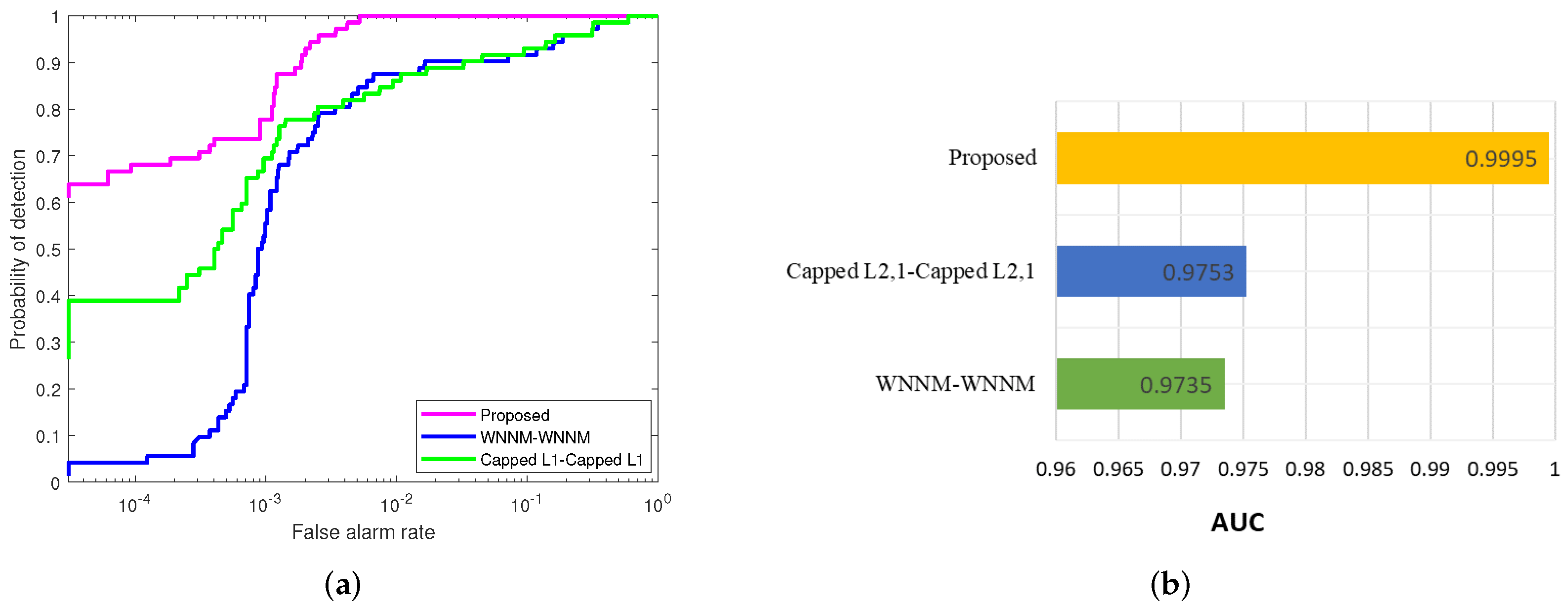
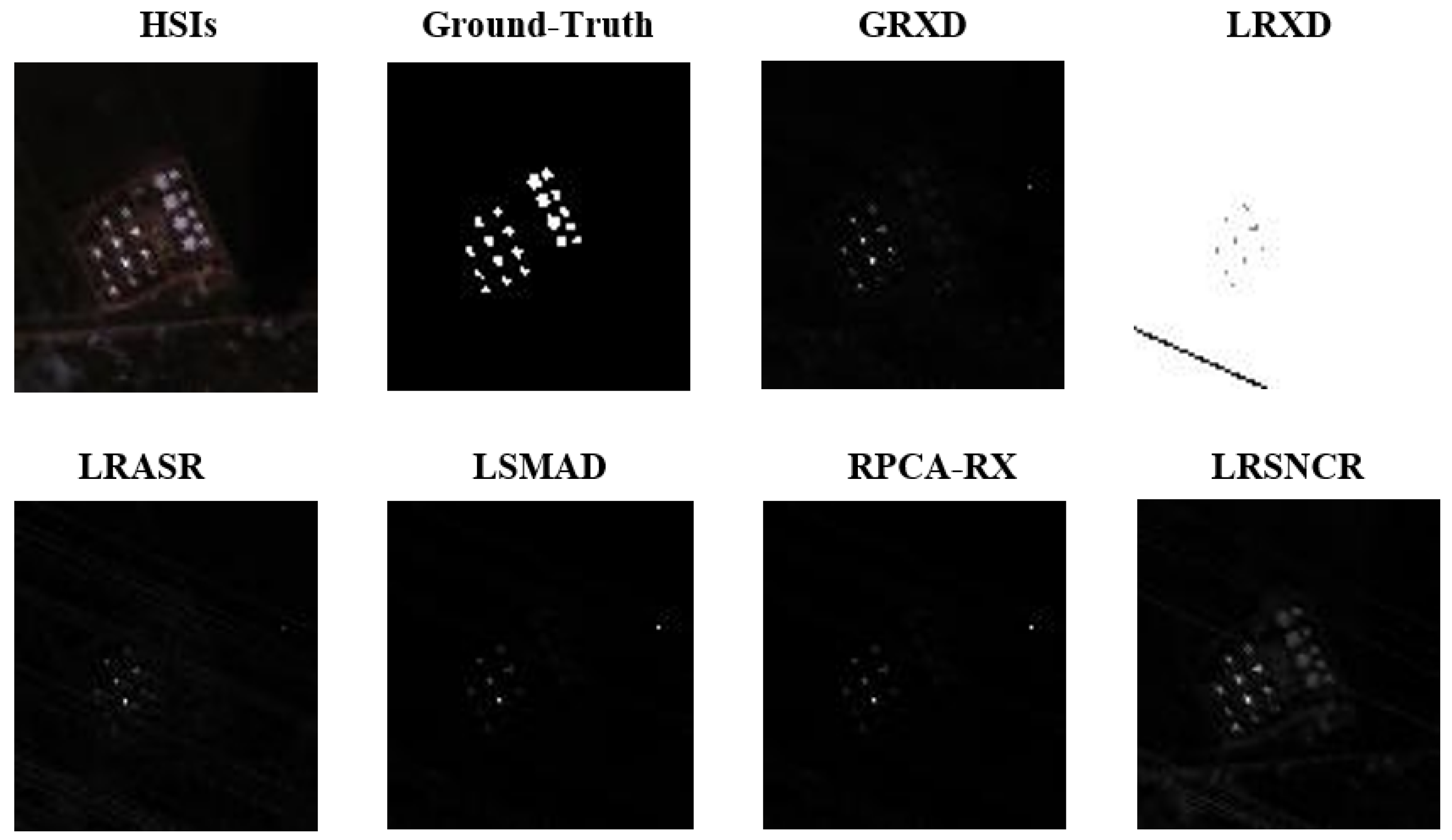
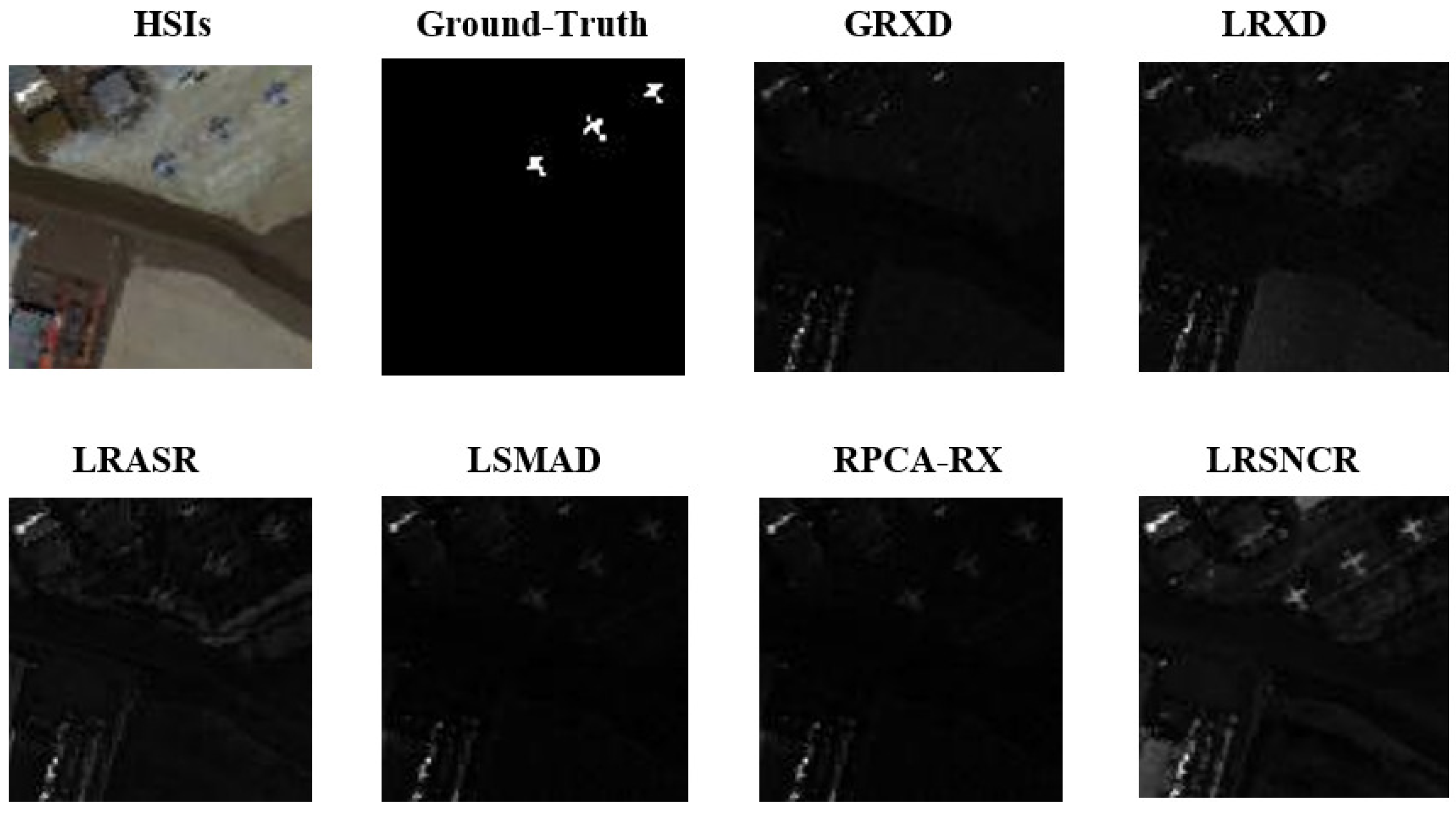
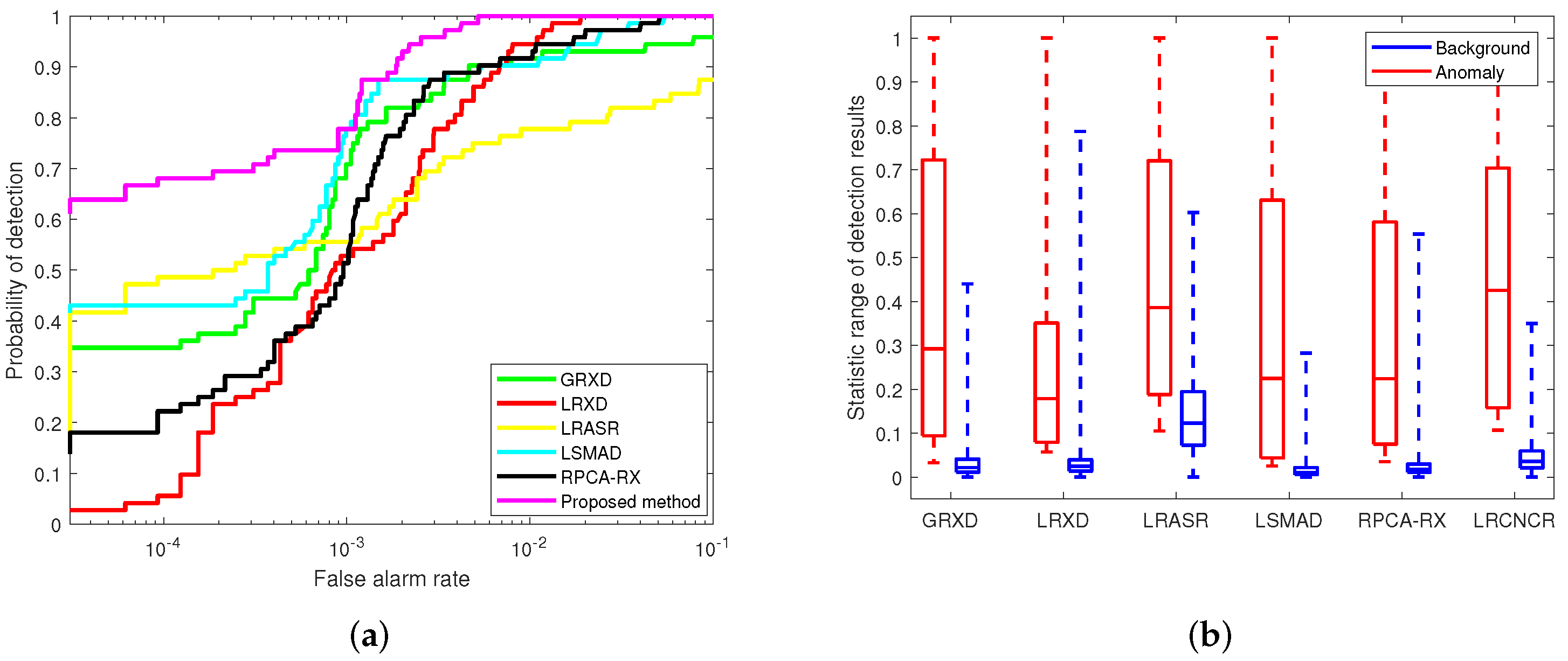
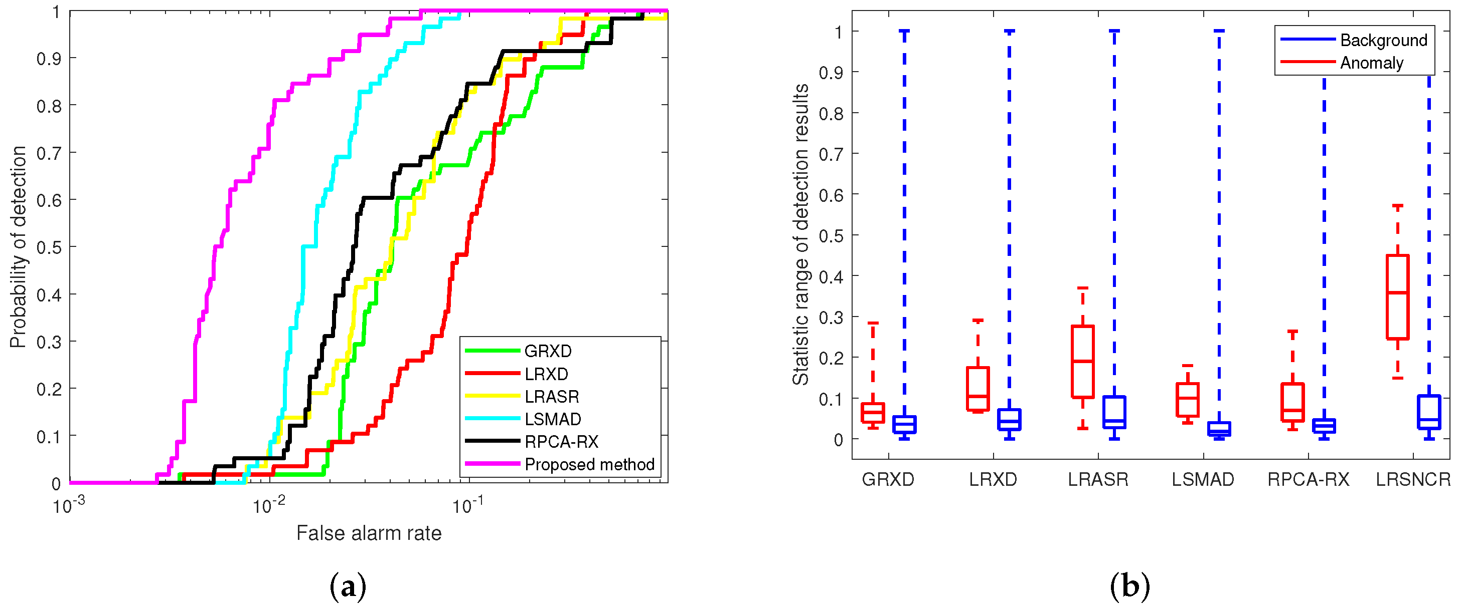
The proposed method adopts improved RPCA models to detect anomalies, anomalies are modeled by the sparse component, and background is modeled by the low-rank component. The experimental results on four real HSI datasets show that the proposed LRSNCR method has better detection performance than other methods and can better separate the background and anomalies.

2. Methodology

In this section, LRSNCR is proposed from HAD in the article and its optimization algorithm is introduced in detail. Firstly, the HSI cube data was rearranged as an input to LRSNCR. Secondly, the anomaly was separated from the background by getting the utmost out of the idea of matrix factorization to solve the problem of constrained convex optimization. Meanwhile, the weighted nuclear norm and Capped ${\ell }_{2,1}$-norm were used to replace the rank function in a low-rank item and the ${\ell }_0$ operator in a sparse item, respectively. Thirdly, the sparse and low-rank components were modeled and solved separately. The proposed LRSNCR architecture is shown in Figure 3.

Figure 3. Flowchart of anomaly detection based on LRSNCR.

Reformulating (1) leads to the following LRSNCR model:

$$\begin{array}{cc}\hfill & \min {∥L∥}_{w,*}+\lambda {∥S∥}_{\stackrel{\wedge }{{\ell }_{2,1}}}\hfill \\ \hfill & s.t.A=L+S\hfill \end{array}$$

(3)

In general, if only Equation (3) is transformed into a convex problem, there are a lot of methods that can be used to solve it. Here, we only introduce an augmented Lagrangian multiplier algorithm, namely Alternating Direction Method of Multipliers (ADMMs [42,43]).

For the optimization problem (3), the augmented Lagrangian function is first constructed:

$$\begin{array}{c}\hfill L(L,S,Y,\mu )={∥L∥}_{w,*}+\lambda {∥S∥}_{\stackrel{\wedge }{{\ell }_{2,1}}}+<Y,A-L-S>+\frac{\mu }{2}{∥A-L-S∥}_F^2\end{array}$$

(4)

where Y is the Lagrangian multiplier, it is the weight of the sparse error term in the cost function, and also is the given parameter, and $\mu$ is a positive scaler. ${∥•∥}_F$ is the Frobenius norm of the matrix when $Y=Y_k,\mu ={\mu }_k$.

Fixed L,Y, update S:

$$\begin{array}{c}\hfill {S_j}^{(k+1)}=\underset{S_j}{\arg \min }L(L^{(k+1)},S_j,Y^{\left(k\right)},{\mu }^{\left(k\right)})\end{array}$$

(5)

The original problem can then be recast into two sub-problems: $q_1$ and $q_2$. This is equivalent to decomposing a non-convex set into two convex sets to solve. The global minimum point is obtained by comparing the local minimum in two convex sets [40].

$$\begin{array}{c}\hfill q_1=\underset{S_j}{\arg \min }\frac{1}{2}{(S_j-u_j)}^2+\frac{\lambda }{\mu }\theta \mathrm{s}.\mathrm{t}.\left|S_j\right|\ge \theta \end{array}$$

(6)

$$\begin{array}{c}\hfill q_2=\underset{S_j}{\arg \min }\frac{1}{2}{(S_j-u_j)}^2+\frac{\lambda }{\mu }\left|S_j\right|\mathrm{s}.\mathrm{t}.\left|S_j\right|<\theta \end{array}$$

(7)

The solutions of $q_1$ and $q_2$ are $e_1$ and $e_1$, respectively, which are the the local minimum points.

$$\begin{array}{c}\hfill e_1=sign\left(u_j\right)\max (\theta ,\left|u_j\right|)\end{array}$$

(8)

$$\begin{array}{c}\hfill e_2=sign\left(u_j\right)\min (\theta ,\max (0,\left|u_j\right|-\lambda /\mu ))\end{array}$$

(9)

The global minimum point is determined by Equation (10).

$$Capped{\ell }_{2,1}:S_j^{(k+1)} = \left\{\begin{array}{c}{e}_1\mathrm{if}{q}_1\left(e_1\right)\le q_1\left(e_2\right)\hfill \\ e_2\mathrm{otherwise}\hfill \end{array}\right.$$

(10)

where, $u_j=\sqrt{{{\displaystyle \sum _j^n}\left[(A-L^{\left(k\right)}+\frac{Y^{\left(k\right)}}{{\mu }^{\left(k\right)}})(i,j)\right]}^2}$ and $\theta$ is a parameter to be set. For each element of $u_j$, $sign\left(u_j\right)$ is the sign function.

Fixed S, Y, update L:

$$\begin{array}{cc}\hfill L^{(k+1)}& =\underset{L}{\arg \min }L(L,S^{(k+1)},Y^{\left(k\right)},{\mu }^{\left(k\right)})\hfill \\ \hfill & =\underset{L}{\arg }\min {∥L∥}_{w,*}+<Y^{\left(k\right)},A-L-S^{\left(k\right)}>+\frac{\mu }{2}{∥A-L-S^{\left(k\right)}∥}_F^2\hfill \\ \hfill & =U\left[\sum _i{w}_i{\sigma }_i\left(L\right)\right]V^T\hfill \end{array}$$

(11)

where ${\displaystyle \sum _i}{w}_i{\sigma }_i\left(L\right)$ is the WNN of matrix L. These include: $w_i$, the weight (zero or positive number), defined for ${\sigma }_i\left(L\right)$ and ${\sigma }_i\left(L\right)$, which is the i-th singular value of matrix L.

In [44], let A = $U\sum V^T$ be the Singular Value Decomposition (SVD) of the observation data A, where $\sum =\left(\begin{array}{c}diag({\sigma }_1\left(A\right),{\sigma }_2\left(A\right),\dots {\sigma }_n\left(A\right))\hfill \\ 0\hfill \end{array}\right)$. If $C\ge 0$, then $\epsilon$ is a small constant satisfying $\epsilon <\min \left\{\sqrt{C},\frac{C}{{\sigma }_i\left(A\right)}\right\}$, the reweighting formula $w_i=\frac{C}{{\sigma }_i^{}\left(L\right)+\epsilon }$, with the initial estimation $L_0$ = A, and the optimization problem $\left\{{\min }_L{∥A-L∥}_F^2+{∥L∥}_{w,*}\right\}$ (WNNM) has the closed-form solution in a low-rank item, which is $\stackrel{\wedge }{L}=U{\displaystyle \sum _{}^{\wedge }}{V}^T$.

Where, ${\displaystyle \sum _{}^{\tilde{}}}=\left(\begin{array}{c}diag({\sigma }_1\left(L^{*}\right),{\sigma }_2\left(L^{*}\right),\dots {\sigma }_n\left(L^{*}\right))\hfill \\ 0\hfill \end{array}\right)$ and

$${\sigma }_i\left(L^{*}\right)=\left\{\begin{array}{c}\begin{array}{cc}0& C_1<0\end{array}\hfill \\ \begin{array}{cc}\frac{C_1+\sqrt{C_2}}{2}& C_2\ge 0\end{array}\hfill \end{array}\right.$$

(12)

$$\begin{array}{c}\hfill C_1={\sigma }_i\left(L\right)-\epsilon \end{array}$$

(13)

$$\begin{array}{c}\hfill C_2={\left({\sigma }_i\left(L\right)+\epsilon \right)}^2-4C\end{array}$$

(14)

Fixed L, S, update Y:

$$\begin{array}{c}\hfill Y^{(k+1)}=Y^{\left(k\right)}+{\mu }^{\left(k\right)}(A-L^{(k+1)}-S^{(k+1)})\end{array}$$

(15)

update $\mu$:

$$\begin{array}{c}\hfill {\mu }^{(k+1)}=\rho {\mu }^{\left(k\right)}\end{array}$$

(16)

where $\mu$ is a positive scaler so that the objective function is only perturbed slightly. Since the LRSNCR model is non-convex for general weight conditions, we used an unbounded ${\mu }_k$ to guarantee the convergence of the proposed method. We did not want the iterations to be stopped very quickly in case ${\mu }_k$ increased too fast, which would be bad for our model. Therefore, in our proposed method, a small value of $\rho$ was used to constrain the problem of excessive growth of ${\mu }_k$.

The LRSNCR is summarized in Algorithm 1 (https://github.com/yoyoath/LRSNCR, accessed on 1 January 2022). Here, the orders of updating L and S can be changed.

Algorithm 1 LRSNCR

Input:$A\in R^{m\times n}$; $\epsilon ,\mu ,\rho$, $\lambda ,\theta ,C>0$; $k_{\max }$ Output: L, S  1: Initializiation: $L_0=0$, $S_0=0$, $Y_0=0$, $k=0$;  2: repeat  3:     Fix other variables as the latest value, and  4: update variable S according to Equations (6)–(10);  5:     Fix other variables as the latest value, and  6: update variable L according to Equations (11)–(14);  7:     Update the Y according to Equation (15);  8:     Update the $\mu$ according to Equation (16);  9: until L and S converges or k > $k_{\max }$

3. Experimentation Results and Discussion

In this section, the availability of the LRSNCR model for HAD is expounded by the analysis and discussion of the experimental results. The algorithms and processes in this paper were implemented using MATLAB language in a PC that was powered by Windows 10 and Core i7-1165 CPU @2.80 GHz by Intel with 16 GB RAM.

3.1. Hyperspectral Datasets

In the experiment, we used some real hyperspectral images to verify the effectiveness of this method in anomaly detection.

(1) ABU(Airport-Beach-Urban)-Urban: The first dataset was from HSI in the ABU dataset, which contained 13 different hyperspectral image scenes, of which Urban was one [45]. These images of size 100 × 100 × 207 were collected on the Rexas Coast, had a resolution of 17.2 m, and were extracted from the Airborne Visible/Infrared Imaging Spectrometer (AVIRIS) website. The anomaly object in this image is a cluster of buildings. The pseudo-color image and ground-truth(GT) map of this dataset is displayed in Figure 4.

Figure 4. ABU-urban dataset and anomaly background response diagram. (a) Pseudo-color image. (b) Ground-truth map.

(2) ABU (Airport-Beach-Urban)-Beach: The second HSI dataset was the beach scenes and consisted of 100 × 100 pixels with 180 bands, and like the source of the first dataset, it was also obtained by (AVIRIS) sensor [46]. Anomalies consisted of man-made reefs in this scene. The pseudo-color image and GT map of this dataset is displayed in Figure 5.

Figure 5. ABU-beach dataset and anomaly background response diagram. (a) Pseudo-color image. (b) Ground-truth map.

(3) SpecTIR: The third experimental data were derived from the SpecTIR hyperspectral airborne Rochester experiment [47]. The detailed experimental information for this dataset was 180 × 180 pixels, 120 bands, 5 nanometer spectral resolution, and 1 meter spatial resolution. In this dataset, noise and useless bands were eliminated in advance where anomalies were forged by artificial-colored textile materials. The pseudo-color image and ground-truth map of this dataset is displayed in Figure 6.

Figure 6. SpecTIR dataset and anomaly background response diagram. (a) Pseudo-color image. (b) Ground-truth map.

(4) Sandiego: The fourth dataset, the San Diego scene, came from the same source as the first two datasets, also provided by (AVIRIS) [48]. The dataset had a spatial resolution of 3.5 and used a partial scene of the Sandiego airport in California (located in the US) in the experiments. The original image contained a total of 224 bands, covering 3,702,510 nm. In total, 189 bands were used in this article. Its space size was 100 × 100 pixels. The three aircraft above the image were considered anomalies, occupying a total of 58 pixels. The pseudo-color image and ground-truth map of this dataset is displayed in Figure 7. As shown in Figure 7a, we selected three bands from 189 bands in the Sandiego dataset to display as pseudo-color images. As shown in Figure 7b, the white pixel was the target or anomaly information, the exception in this image was the aircraft, and the background was a black pixel. It was used to compare with our test results.

Figure 7. Sandiego dataset and anomaly background response diagram. (a) Pseudo-color image. (b) Ground-truth map.

3.2. Evaluation Metrics and Parameter Tuning

3.2.1. Evaluation Metrics

We introduced the detection map, anomaly background separability map, ROC curve, and AUC value to carry out a qualitative and quantitative analysis of LRSNCR [49]. The anomaly background separability map and detection map can qualitatively evaluate the proposed detection performance of LRSNCR.

The ROC curve is a quantitative HAD and evaluation technical index based on the anomaly target reference information provided in the true value map marked by the anomaly point position in the hyperspectral image, and the detection results obtained by the HAD method were based on the detection value. In general, the false alarm rate (FAR) was used as the abscissa and the probability of detection (PD) was used as the ordinate in the ROC curve, respectively.

The definition of FAR and PD is:

$$\mathrm{FAR}=\frac{N_{fd}}{N_a}$$

(17)

$$\mathrm{PD}=\frac{N_{cd}}{N_t}$$

(18)

where $N_{fd}$ symbolizes the background pixel counts that are incorrectly judged as anomaly pixel counts and $N_a$ symbolizes the total counts of pixels in HSI. $N_{cd}$ represents the detected anomaly pixel counts and $N_t$ represents the total counts of anomaly target pixel in the HSI.

The AUC value is often used as an important performance assessment indicator to estimate the algorithm performance under different parameters. Ideally, this value is 1. The closer the value is to 1, the better the algorithm performance under this parameter. The calculation formula of AUC is:

$$\mathrm{AUC}={\int }_0^{+\infty }{F}_{\mathrm{ROC}}\left(x\right)dx$$

(19)

where $F_{\mathrm{ROC}}$ represents the ROC curve function.

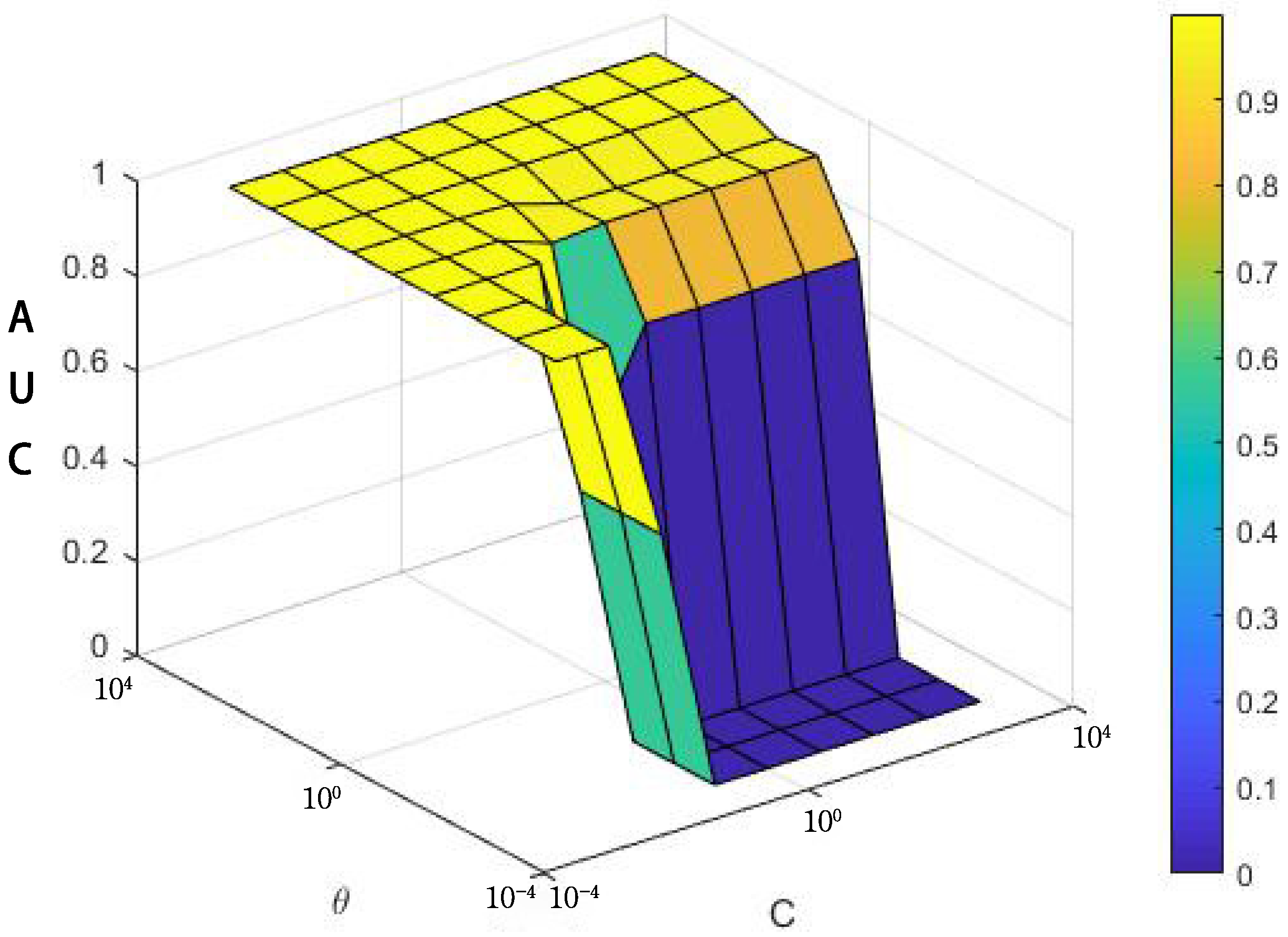
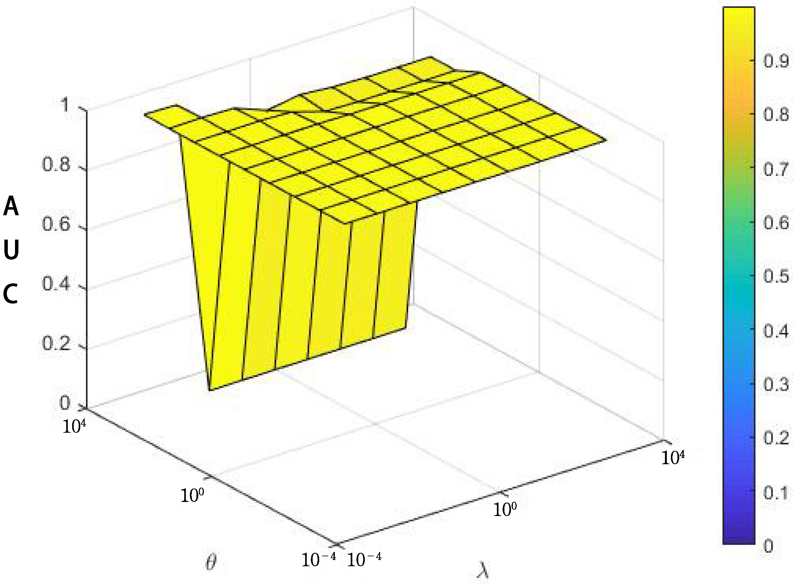
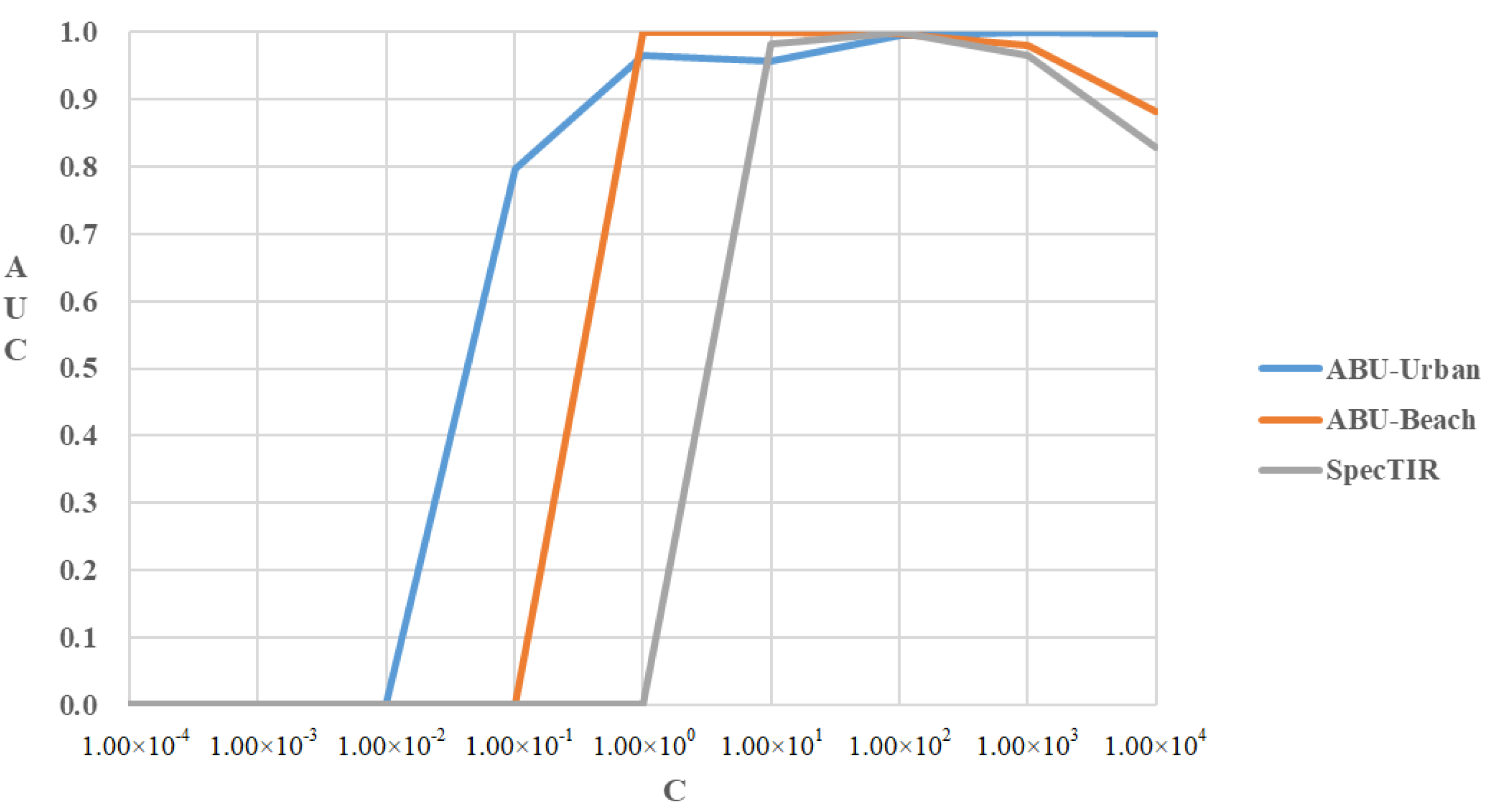
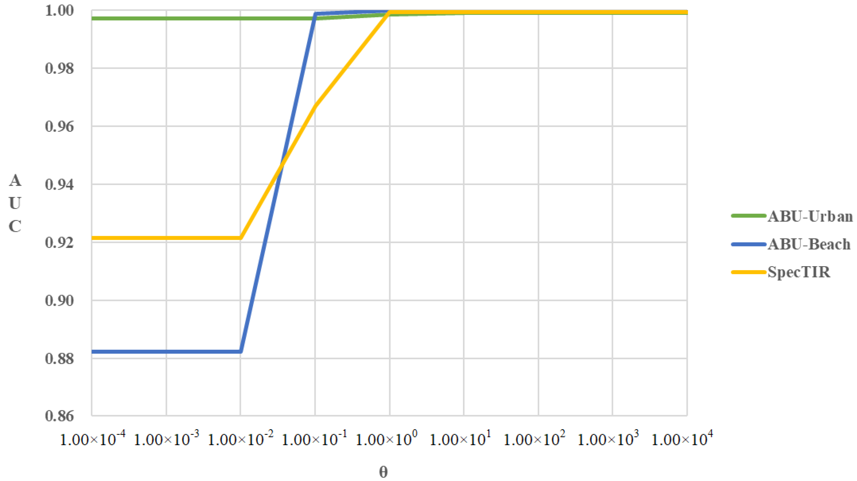
3.2.2. Parameter Tuning

LRSNCR had some parameters to tune, including the weighted C in WNNM and other parameters ($\rho$, $\lambda$, and $\theta$). With AUC as the evaluation index, we tested the effect of different parameters on the performance of LRSNCR on ABU-Urban, ABU-Beach, and SpecTIR datasets.

In our proposed method, $\rho$ was not a very large value, according to prior knowledge and the previous chapter. Thus, we searched the best $\rho$, varying from 0.5 to 1.5 at intervals of 0.05 in Figure 8. In all datasets, we found that the detection performance was very poor when $\rho$ was between 0.5 and 1.05 (short of 1.05). When $\rho$ reached 1.05, the AUC value was higher and the detection performance was the best. Therefore, in all subsequent experiments, the $\rho$ of LRSNCR was set to a fixed value of 1.05.

Figure 8. Tuning $\rho$ of the proposed LRSNCR.

We also dynamically adjusted the influence of different C, $\lambda$, and $\theta$ changes on AUC. They were fixed on a scale of $\left\{\left.{10}^{-4},{10}^{-3},{10}^{-2},{10}^{-1},{10}^0,{10}^1,{10}^2,{10}^3,{10}^4\right\}\right.$, respectively. Firstly, C and $\theta$ were tuned with other parameters fixed in Figure 9. Then $\lambda$ and $\theta$ were tuned with other parameters fixed in Figure 10. The parameters adjustment process in this part was all carried out in the ABU-Urban dataset.

Figure 9. Tuning C and $\theta$ of the proposed LRSNCR in the ABU-urban dataset.

Figure 10. Tuning $\lambda$ and $\theta$ of the proposed LRSNCR in the ABU-urban dataset.

Aiming to further study the effect of these three parameters for AUC values, the different effects of each parameter for AUC values were explored on three datasets, which are shown in Figure 11, Figure 12 and Figure 13. It was observed that the weighted C was more sensitive than the $\lambda$ and $\theta$ parameters according to AUC value. Therefore, in the following experiments, in all datasets, $\lambda$ was 1 and $\theta$ was 10, respectively, and the parameter C still needed to be adjusted separately in each datasets to obtain a better good experimental results.

Figure 11. Tuning C of the proposed LRSNCR.

Figure 12. Tuning $\lambda$ of the proposed LRSNCR.

Figure 13. Tuning $\theta$ of the proposed LRSNCR.

3.3. Detection Performance and Discussion

We analyzed the detection performance in our proposed LRSNCR, which done using two sets of comparative experiments. Firstly, the fixed low-rank term remained unchanged using the WNNM method, and some mainstream penalty functions were selected to replace the ${\ell }_0$ operator in the sparse item, such as SCAD, MCP, and ${\ell }_{2,1}$, and were called WNNM-SCAD, WNNM-MCP, and WMMN-L2,1. In addition, the same method (WNNM or Capped ${\ell }_{2,1}$) was used to replace the rank function of the low-rank term and the ${\ell }_0$ operator in the sparse item, which was named WNNM-WNNM, Capped L2,1-Capped L2,1. Using SpecTIR dataset as an example, we evaluated their detection capabilities based on ROC and AUC.

Figure 14a and Figure 15a show that the ROC curve of the LRSNCR algorithm almost wrapped the curves of other methods, indicating that the performance of the LRSNCR algorithm on the ROC curve far exceeded the other methods. In Figure 14b and Figure 15b, AUC values of the proposed LRSNCR were also relatively high. Therefore, whether for the low-rank item using the Capped ${\ell }_{2,1}$-norm or the sparse item using other penalty functions (or WNNM), the LRSNCR had the better detection performance.

Figure 14. Visualizing ROC curves and AUC values in the SpecTIR dataset. (a) ROC curves. (b) AUC values.

Figure 15. Visualizing ROC curves and AUC values in the SpecTIR dataset. (a) ROC curves. (b) AUC values.

Secondly, to further analyze the detection of performance based on the proposed LRSNCR, we contrasted the detection performance between some classical hyperspectral image anomaly detection methods, such as GRXD [13], LRXD [15], and LRaSMD-based methods, such as LRASR [24], LSMAD [23], and RPCA-RX [27].

Figure 16, Figure 17, Figure 18 and Figure 19 illustrate the detection diagrams by the different methods on each datasets. The higher the value in the graph, the brighter the pixel, which means the greater the chance of being an anomaly pixel. As shown in Figure 16, our proposed method could detect most of the anomalies in the dataset and could better suppress the background. Other methods can only detect some anomaly, and LRXD has the worst detection performance. In Figure 17 and Figure 18, although all methods could detect anomalies, it was obvious that only our method had the lowest FAR. In Figure 19, only our proposed method could fully detect the three aircraft located in the top right-hand corner, while others could not. Therefore, it can be concluded that the proposed LRSNCR is superior to other methods, with a better capability of separating background from anomaly.

Figure 16. Detection maps by ABU-urban dataset.

Figure 17. Detection maps by ABU-beach dataset.

Figure 18. Detection maps by SpecTIR dataset.

Figure 19. Detection maps by Sandiego dataset.

Figure 20, Figure 21, Figure 22 and Figure 23 illustrate the ROC curves and Separability map obtained by different methods for each dataset. Figure 20a, Figure 21a, Figure 22a and Figure 23a stand for ROC curves and Figure 20b, Figure 21b, Figure 22b and Figure 23b represent box-plots for each real hypserspectral dataset.

Figure 20. ROC curves and separability map acquired through the ABU-urban dataset. (a) ROC curves. (b) Box-plot.

Figure 21. ROC curves and separability map acquire through the ABU-beach dataset. (a) ROC curves. (b) Box-plot.

Figure 22. ROC curves and Separability map acquire through the SpecTIR dataset. (a) ROC curves. (b) Box-plot.

Figure 23. ROC curves and separability map acquire through the Sandiego dataset. (a) ROC curves. (b) Box-plot.

As shown in Figure 20a, the PD of LRSNCR was bigger than others in the beginning. After continuing, LRSNCR still had a high probability detection and low FAR. The curves produced by GRXD, LSMAD, and RPCA-RX were intertwined and mediocre, while LRXD and LRASR tended to be closer to the bottom right and performed less well. As shown in Figure 21a, the curve produced by LRSNCR demonstrated a higher PD and a lower FAR than the other detection methods. LRSNCR had a FAR of approximately 0.001 while achieving a 100% probability of detection. Therefore, it was more convincing than others. In Figure 22a, the curve of LRSNCR had a significant trend, wrapping the other curves, and the rest of the curves were intertwined, except for the LRSNCR. In addition, after FAR = 0.008, the LRSNCR had a larger PD. In comparison with others, LRSNCR was at an obvious advantage. As shown in Figure 23a, the curves of GRXD, LRXD, LRASR, LSMAD, and RPCA-RX were also intertwined, which meant that the effect of LSMAD was better but not as good as that of LRSNCR. These curves were always below that produced by LRSNCR. Almost all of the ROC curves of the LRSNCR method can wrap around those of other methods, with a higher detection rate but a lower FAR. This shows that the performance of LRSNCR method on ROC curve is much better than that of other methods.

In the box-plot, after first processing the data regarding anomaly and background, two rectangles of the separability graph were obtained, in which red rectangle indicated the anomaly and the blue rectangle indicated the background. The separability between the anomaly and the background was determined by the distance between the red and blue rectangles. The larger distance between red and blue rectangles of LRSNCR than that of other comparison methods, as shown in Figure 20b, indicates that LRSNCR can better separate anomalies from the background and is more convincing. The box-plot shown in Figure 21b, Figure 22b and Figure 23b, also indicates that the proposed LRSNCR can easily identify desired anomalies from background.

Table 2 lists the objective index AUC values obtained by anomaly detection of each data set by different methods. The AUC for the proposed LRSNCR on the four datasets were 0.9991, 0.9999, 0.9995, and 0.9903, respectively. Furthermore, the second largest AUC values on the four datasets were 0.9957, 0.9998, 0.9976, and 0.9778, which were not higher than our method. In each hyperspectral data set, the execution time of proposed method was 49.83561, 22.08689, 27.86498, and 19.45832, respectively. Table 3 provides the execution time of various detection methods. We proposed LRSNCR to be in the middle and lower level in execution time and did not have much advantage in computing time, because our method requires iterative optimization.

Table 2. The contrast in AUC from six anomaly detection methods.

Methods	GRXD	LRXD	LRASR	LSMAD	RPCA-RX	Proposed
ABU-Urban	0.9946	0.5713	0.8385	0.9843	0.9957	0.9991
ABU-Beach	0.9998	0.9736	0.9990	0.9995	0.9995	0.9999
SpecTIR	0.9914	0.9976	0.9685	0.9972	0.9971	0.9995
Sandiego	0.8886	0.8892	0.9200	0.9778	0.9165	0.9903

Table 3. The running time (unit:s) of different methods using four experimental datasets.

Methods	GRXD	LRXD	LRASR	LSMAD	RPCA-RX	Proposed
ABU-Urban	0.06351	69.55086	71.08300	24.96805	12.74864	49.83561
ABU-Beach	0.05629	39.46180	33.64385	9.85913	3.24897	22.08689
SpecTIR	0.10012	94.28799	89.25651	20.59356	4.78673	27.86498
Sandiego	0.15725	39.23523	32.22894	10.89012	3.41575	19.45832

4. Conclusions

In this article, an improved RPCA with non-convex regularized was proposed for HAD through the research and improvement of the RPCA problem. The rank norm and the ${\ell }_0$ operator were replaced with the WNNM and non-convex Capped ${\ell }_{2,1}$-norm. Experiments with four hyperspectral datasets demonstrated that, by using the LRSNCR method, discrimination between anomalies and background was enhanced. Compared with classical GRXD, LRXD and LRASR and LSMAD and RPCA-RX detectors in four real hyperspectral datasets, it was still better than others in terms of detection effectiveness and stability by the proposed LRSNCR.

The proposed method, based on low-rank and sparse joint non-convex regularization, was different from many improvements based on low-rank or sparse terms. Experimental results also show that our method achieved good results but still has some limitations. When dealing with large-scale hyperspectral image data, the iterative optimization speed of the algorithm may be less dominant, so reducing the running time or speeding up the convergence speed is an important aspect worth considering. In recent years, tensor-based and deep learning-based methods have been widely used in hyperspectral anomaly detection. In the future, we will consider low-rank approximation and deep learning or methods combined with tensors.

References

- Bioucas-Dias, J.M.; Plaza, A.; Camps-Valls, G.; Scheunders, P.; Nasrabadi, N.; Chanussot, J. Hyperspectral Remote Sensing Data Analysis and Future Challenges. IEEE Geosci. Remote Sens. Mag. 2013, 1, 6–36. [Google Scholar] [CrossRef] [Green Version]
- Jiang, M.; Fang, Y.; Su, Y.; Cai, G.; Han, G. Random Subspace Ensemble With Enhanced Feature for Hyperspectral Image Classification. IEEE Geosci. Remote Sens. Lett. 2020, 17, 1373–1377. [Google Scholar] [CrossRef]
- Li, W.; Du, Q. Collaborative Representation for Hyperspectral Anomaly Detection. IEEE Trans. Geosci. Remote Sens. 2015, 53, 1463–1474. [Google Scholar] [CrossRef]
- Su, Y.; Xu, X.; Li, J.; Qi, H.; Gamba, P.; Plaza, A. Deep Autoencoders With Multitask Learning for Bilinear Hyperspectral Unmixing. IEEE Trans. Geosci. Remote Sens. 2020, 59, 8615–8629. [Google Scholar] [CrossRef]
- Zhu, X.; Cao, L.; Wang, S.; Gao, L.; Zhong, Y. Anomaly Detection in Airborne Fourier Transform Thermal Infrared Spectrometer Images Based on Emissivity and a Segmented Low-Rank Prior. Remote Sens. 2021, 13, 754. [Google Scholar] [CrossRef]
- Shimoni, M.; Haelterman, R.; Perneel, C. Hypersectral Imaging for Military and Security Applications: Combining Myriad Processing and Sensing Techniques. IEEE Geosci. Remote Sens. Mag. 2019, 7, 101–117. [Google Scholar] [CrossRef]
- Zhao, X.; Hou, Z.; Wu, X.; Li, W.; Ma, P.; Tao, R. Hyperspectral target detection based on transform domain adaptive constrained energy minimization. Int. J. Appl. Earth Obs. Geoinf. 2021, 103, 102461. [Google Scholar] [CrossRef]
- Liu, J.; Hou, Z.; Li, W.; Tao, R.; Orlando, D.; Li, H. Multipixel Anomaly Detection With Unknown Patterns for Hyperspectral Imagery. IEEE Trans. Neural Netw. Learn. Syst. 2021, 1–11. [Google Scholar] [CrossRef]
- Hou, Z.; Wei, L.; Tao, R.; Shi, W. Collaborative Representation with Background Purification and Saliency Weight for Hyperspectral Anomaly Detection. Sci. China Inf. Sci. 2022, 65, 112305. [Google Scholar] [CrossRef]
- Zhao, R.; Du, B.; Zhang, L. A Robust Nonlinear Hyperspectral Anomaly Detection Approach. IEEE J. Sel. Top. Appl. Earth Obs. Remote Sens. 2014, 7, 1227–1234. [Google Scholar] [CrossRef]
- Du, B.; Zhang, L. Random-Selection-Based Anomaly Detector for Hyperspectral Imagery. IEEE Trans. Geosci. Remote Sens. 2011, 49, 1578–1589. [Google Scholar] [CrossRef]
- Zhao, C.; Li, C.; Feng, S. A Spectral–Spatial Method Based on Fractional Fourier Transform and Collaborative Representation for Hyperspectral Anomaly Detection. IEEE Geosci. Remote Sens. Lett. 2021, 18, 1259–1263. [Google Scholar] [CrossRef]
- Reed, I.; Yu, X. Adaptive multiple-band CFAR detection of an optical pattern with unknown spectral distribution. IEEE Trans. Acoust. Speech Signal Process. 1990, 38, 1760–1770. [Google Scholar] [CrossRef]
- Zhao, C.; Li, C.; Feng, S.; Su, N.; Li, W. A Spectral–Spatial Anomaly Target Detection Method Based on Fractional Fourier Transform and Saliency Weighted Collaborative Representation for Hyperspectral Images. IEEE J. Sel. Top. Appl. Earth Obs. Remote Sens. 2020, 13, 5982–5997. [Google Scholar] [CrossRef]
- Borghys, D.; Kasen, I.; Achard, V.; Perneel, C.; Shen, S.S.; Lewis, P.E. Comparative evaluation of hyperspectral anomaly detectors in different types of background. Int. Soc. Opt. Photonics 2012, 8390, 83902J. [Google Scholar]
- Guo, Q.; Zhang, B.; Ran, Q.; Gao, L.; Li, J.; Plaza, A. Weighted-RXD and Linear Filter-Based RXD: Improving Background Statistics Estimation for Anomaly Detection in Hyperspectral Imagery. IEEE J. Sel. Top. Appl. Earth Obs. Remote Sens. 2014, 7, 2351–2366. [Google Scholar] [CrossRef]
- Kwon, H.; Nasrabadi, N. Kernel RX-algorithm: A nonlinear anomaly detector for hyperspectral imagery. IEEE Trans. Geosci. Remote Sens. 2005, 43, 388–397. [Google Scholar] [CrossRef]
- Khazai, S.; Homayouni, S.; Safari, A.; Mojaradi, B. Anomaly Detection in Hyperspectral Images Based on an Adaptive Support Vector Method. IEEE Geosci. Remote Sens. Lett. 2011, 8, 646–650. [Google Scholar] [CrossRef]
- Matteoli, S.; Diani, M.; Corsini, G. Hyperspectral Anomaly Detection With Kurtosis-Driven Local Covariance Matrix Corruption Mitigation. IEEE Geosci. Remote Sens. Lett. 2011, 8, 532–536. [Google Scholar] [CrossRef]
- Du, L.; Wu, Z.; Xu, Y.; Liu, W.; Wei, Z. Kernel low-rank representation for hyperspectral image classification. In Proceedings of the 2016 IEEE International Geoscience and Remote Sensing Symposium (IGARSS), Beijing, China, 10–15 July 2016; pp. 477–480. [Google Scholar] [CrossRef]
- Li, L.; Li, W.; Du, Q.; Tao, R. Low-Rank and Sparse Decomposition With Mixture of Gaussian for Hyperspectral Anomaly Detection. IEEE Trans. Cybern. 2021, 51, 4363–4372. [Google Scholar] [CrossRef]
- Zhou, T.; Tao, D. GoDec: Randomized Lowrank & Sparse Matrix Decomposition in Noisy Case. In Proceedings of the International Conference on Machine Learning, Bellevue, WA, USA, 28 June–2 July 2011. [Google Scholar]
- Zhang, Y.; Du, B.; Zhang, L.; Wang, S. A Low-Rank and Sparse Matrix Decomposition-Based Mahalanobis Distance Method for Hyperspectral Anomaly Detection. IEEE Trans. Geosci. Remote Sens. 2016, 54, 1376–1389. [Google Scholar] [CrossRef]
- Xu, Y.; Wu, Z.; Li, J.; Plaza, A.; Wei, Z. Anomaly Detection in Hyperspectral Images Based on Low-Rank and Sparse Representation. IEEE Trans. Geosci. Remote Sens. 2016, 54, 1990–2000. [Google Scholar] [CrossRef]
- Zhang, X.; Wen, G.; Dai, W. A Tensor Decomposition-Based Anomaly Detection Algorithm for Hyperspectral Image. IEEE Trans. Geosci. Remote Sens. 2016, 54, 5801–5820. [Google Scholar] [CrossRef]
- Candès, E.J.; Li, X.; Ma, Y.; Wright, J. Robust Principal Component Analysis? J. ACM 2011, 58, 1–37. [Google Scholar] [CrossRef]
- Sun, W.; Liu, C.; Li, J.; Lai, Y.M.; Li, W. Low-rank and sparse matrix decomposition-based anomaly detection for hyperspectral imagery. J. Appl. Remote Sens. 2014, 8, 083641. [Google Scholar] [CrossRef]
- Li, F.R. Variable Selection via Nonconcave Penalized Likelihood and its Oracle Properties. Publ. Am. Stat. Assoc. 2001, 96, 1348–1360. [Google Scholar]
- Zhang, C.H. Nearly unbiased variable selection under minimax concave penalty. Ann. Stat. 2010, 38, 894–942. [Google Scholar] [CrossRef] [Green Version]
- Zhao, X.; Li, W.; Zhang, M.; Tao, R.; Ma, P. Adaptive Iterated Shrinkage Thresholding-Based Lp-Norm Sparse Representation for Hyperspectral Imagery Target Detection. Remote Sens. 2020, 12, 3991. [Google Scholar] [CrossRef]
- Candès, E.; Wakin, M.B.; Boyd, S.P. Enhancing Sparsity by Reweighted ℓ1 Minimization. J. Fourier Anal. Appl. 2008, 14, 877–905. [Google Scholar] [CrossRef]
- Trzasko, J.; Manduca, A. Highly Undersampled Magnetic Resonance Image Reconstruction via Homotopic ℓ0-Minimization. IEEE Trans. Med. Imaging 2009, 28, 106–121. [Google Scholar] [CrossRef]
- Gong, P.; Ye, J.; Zhang, C. Multi-stage multi-task feature learning. Adv. Neural Inf. Process. Syst. 2012, 25. Available online: https://proceedings.neurips.cc/paper/2012/hash/2ab56412b1163ee131e1246da0955bd1-Abstract.html (accessed on 1 January 2022).
- Abadía-Heredia, R.; López-Martín, M.; Carro, B.; Arribas, J.; Pérez, J.; Le Clainche, S. A predictive hybrid reduced order model based on proper orthogonal decomposition combined with deep learning architectures. Expert Syst. Appl. 2022, 187, 115910. [Google Scholar] [CrossRef]
- Lopez-Martin, M.; Le Clainche, S.; Carro, B. Model-free short-term fluid dynamics estimator with a deep 3D-convolutional neural network. Expert Syst. Appl. 2021, 177, 114924. [Google Scholar] [CrossRef]
- Recht, B.; Fazel, M.; Parrilo, P.A. Guaranteed Minimum-Rank Solutions of Linear Matrix Equations via Nuclear Norm Minimization. SIAM Rev. 2010, 52, 471–501. [Google Scholar] [CrossRef] [Green Version]
- Lu, C.; Zhu, C.; Xu, C.; Yan, S.; Lin, Z. Generalized Singular Value Thresholding. Comput. Sci. 2014, 29, 8123533. [Google Scholar]
- Fazel, M. Matrix Rank Minimization with Applications. Ph.D. Thesis, Stanford University, Stanford, CA, USA, 2002. [Google Scholar]
- Gu, S.; Xie, Q.; Meng, D.; Zuo, W.; Feng, X.; Zhang, L. Weighted Nuclear Norm Minimization and Its Applications to Low Level Vision. Int. J. Comput. Vis. 2017, 121, 183–208. [Google Scholar] [CrossRef]
- Gong, P.; Zhang, C.; Lu, Z.; Huang, J.Z.; Ye, J. A General Iterative Shrinkage and Thresholding Algorithm for Non-Convex Regularized Optimization Problems. In Proceedings of the 30th International Conference on International Conference on Machine Learning, Atlanta, GA, USA, 17–19 June 2013; Volume 28, pp. 37–45. [Google Scholar]
- Lu, C.; Tang, J.; Yan, S.; Lin, Z. Nonconvex Nonsmooth Low Rank Minimization via Iteratively Reweighted Nuclear Norm. IEEE Trans. Image Process. 2016, 25, 829–839. [Google Scholar] [CrossRef] [Green Version]
- Boyd, S.; Parikh, N.; Chu, E.; Peleato, B.; Eckstein, J. Distributed Optimization and Statistical Learning via the Alternating Direction Method of Multipliers. Found. Trends Mach. Learn. 2011, 3, 1–122. [Google Scholar] [CrossRef]
- Eckstein, J.; Yao, W. Understanding the convergence of the alternating direction method of multipliers: Theoretical and computational perspectives. Pac. J. Optim. 2015, 11, 619–644. [Google Scholar]
- Huang, X.; Du, B.; Tao, D.; Zhang, L. Spatial-Spectral Weighted Nuclear Norm Minimization for Hyperspectral Image Denoising. Neurocomputing 2020, 399, 271–284. [Google Scholar] [CrossRef]
- Kang, X.; Zhang, X.; Li, S.; Li, K.; Li, J.; Benediktsson, J.A. Hyperspectral Anomaly Detection With Attribute and Edge-Preserving Filters. IEEE Trans. Geosci. Remote Sens. 2017, 55, 5600–5611. [Google Scholar] [CrossRef]
- Li, L.; Li, W.; Qu, Y.; Zhao, C.; Tao, R.; Du, Q. Prior-Based Tensor Approximation for Anomaly Detection in Hyperspectral Imagery. IEEE Trans. Neural Netw. Learn. Syst. 2020, 33, 1037–1050. [Google Scholar] [CrossRef] [PubMed]
- Herweg, J.A.; Kerekes, J.P.; Weatherbee, O.; Messinger, D.; Aardt, J.V.; Ientilucci, E.; Ninkov, Z.; Faulring, J.; Raqueño, N.; Meola, J. SpecTIR hyperspectral airborne Rochester experiment data collection campaign. Spie Def. Secur. Sens. 2012, 8390, 839028. Available online: https://scholar.archive.org/work/ombukmvtczevtarnvfnf5yx64u/access/wayback/http://twiki.cis.rit.edu/twiki/pub/Main/ShareSpecTIR/SHARE_Report_v10.pdf (accessed on 1 January 2022).
- Zhao, R.; Du, B.; Zhang, L. Hyperspectral Anomaly Detection via a Sparsity Score Estimation Framework. IEEE Trans. Geosci. Remote Sens. 2017, 55, 3208–3222. [Google Scholar] [CrossRef]
- Hou, Z.; Li, W.; Li, L.; Tao, R.; Du, Q. Hyperspectral Change Detection Based on Multiple Morphological Profiles. IEEE Trans. Geosci. Remote Sens. 2021, 60, 5507312. [Google Scholar] [CrossRef]
Publisher’s Note: MDPI stays neutral with regard to jurisdictional claims in published maps and institutional affiliations. |
© 2022 by the authors. Licensee MDPI, Basel, Switzerland. This article is an open access article distributed under the terms and conditions of the Creative Commons Attribution (CC BY) license (https://creativecommons.org/licenses/by/4.0/).