Locality Constrained Low Rank Representation and Automatic Dictionary Learning for Hyperspectral Anomaly Detection

Abstract

Hyperspectral anomaly detection (HAD) as a special target detection can automatically locate anomaly objects whose spectral information are quite different from their surroundings, without any prior information about background and anomaly. In recent years, HAD methods based on the low rank representation (LRR) model have caught much attention, and achieved good results. However, LRR is a global structure model, which inevitably ignores the local geometrical information of hyperspectral image. Furthermore, most of these methods need to construct dictionaries with clustering algorithm in advance, and they are carried out stage by stage. In this paper, we introduce a locality constrained term inspired by manifold learning topreserve the local geometrical structure during the LRR process, and incorporate the dictionary learning into the optimization process of the LRR. Our proposed method is an one-stage algorithm, which can obtain the low rank representation coefficient matrix, the dictionary matrix, and the residual matrix referring to anomaly simultaneously. One simulated and three real hyperspectral images are used as test datasets. Three metrics, including the ROC curve, AUC value, and box plot, are used to evaluate the detection performance. The visualized results demonstrate convincingly that our method can not only detect anomalies accurately, but also suppress the background information and noises effectively. The three evaluation metrics also prove that our method is superior to other typical methods.

1. Introduction

As a 3D data cube, hyperspectral image (HSI) contains both spatial and spectral information. It usually consists of hundreds of narrow spectral bands ranging from the visible to the infrared spectrum [1]. The abundant spectral information offers an unique ability to analyze physicochemical characteristics of materials, which possesses great advantages in many remote sensing applications such as change detection [2], scene classification [3], and target detection [4].

Hyperspectral anomaly detection (HAD) [5] is an important branch of target detection. As opposed to matching target detection [6] with known information, HAD can automatically locate anomaly objects without any prior knowledge. In general, anomaly objects are thought distinctive and abnormal. And they have these characteristics: low proportion, small-size, and large spectral difference from the entire background or their surrounding pixels [7]. Anomaly objects have various entities depending on the application scenario. For example, anomaly objects are man-made objects in aerial reconnaissance [8,9,10], and interesting minerals in geological exploration [11].

In past decades, many HAD algorithms have been proposed. The most classical one is the Reed-Xiaoli (RX) algorithm [12], which is considered a benchmark. The RX algorithm assumes that the background data conforms to a Gaussian distribution, and anomaly degree of a pixel can be obtained by computing its deviation degree from the background distribution. There are two versions of RX algorithm: global RX (GRX) and local RX (LRX) [12]. The LRX adopts a slide dual-window model to find anomalies block by block. However, the multivariate Gaussian distribution is unable to model complex background, and the background modeling may be contaminated by anomalies [5]. There are two common strategies to improve the RX algorithm. One is to enhance the background pixels selection or remove anomalies for a relative pure background. In [13], the weighted RX algorithm assigns larger weight to suspected background pixels, in order to reduce the impact of anomaly pixels. In [14], a locally adaptable iterative RX algorithm was presented, which removes suspected anomaly pixels with RX algorithm iteratively until the results make approximately no change. In [15], the spectral angle distance between each pixel vector and the mean of all pixels are computed, and then the pixels with larger distance are removed to obtain a purer background. The other is kernel technique. Kwon et al. proposed the kernel RX (KRX) [16] method, which enlarges the separation degree between the anomaly and background by mapping nonlinearly the image to a higher-dimensional space. On account of its high computational complexity, a cluster kernel RX algorithm [17] was proposed further, which classifies the original data into several clusters and then adopts KRX method in each cluster.

Recently, the representation-based HAD methods have drawn much attention. The sparse representation (SR)-based HAD method assumes that a background pixel can be linearly expressed by a dictionary with corresponding spare vector [18], but anomaly pixel can not. In [19], a method by the use of background joint sparse representation (BJSR) method was presented, which employs a triple-window model and joint sparse representation to build a representative background dictionary. In [20], a multi-dictionary SR with discriminative feature learning was proposed. The collaborative-representation-based (CRD) detector [21] considers that each background pixel can be well expressed by its spatial neighbors, while anomalies can not. Following that, a background refinement collaboration representation method [22] was developed, where background pixels are obtained according to representation coefficients. Furthermore, the low rank representation (LRR)-based methods have been introduced, which seeks the low rank representation of a HSI. In [23], a low-rank and sparse matrix decomposition-based (LRaSMD) anomaly detection algorithm was proposed, in which the Go Decomposition algorithm [24] was used to decompose original HSI. On the basis of the LRaSMD method, Zhang et al. [25] proposed a LRaSMD-based Mahalanobis-distance anomaly detector (LSMAD), where a robust background is obtained by the LRaSMD method. In [26], the abundance map obtained by spectral unmixing algorithm was fed into a LRR model instead of original HSI, and the dictionary was constructed with a clustering algorithm. In [27], a low rank and sparse representation (LRASR)-based detection method was presented. It employed a sparse regularization term to constrain the representation coefficient matrix, and the dictionary was also constructed by the clustering algorithm. In [28], a anomaly detector using graph dictionary-based low rank decomposition with texture feature extraction is proposed, in which the dictionary was constructed by the graph Laplacian matrix.

Although the methods based on the LRR model can effectively model the background and anomaly part, there are still some drawbacks. Firstly, LRR is a global structure model [29,30], which inevitably ignores the local geometrical information. As we all know, the local structure information is beneficial to target detection [31]. Secondly, most LRR-based HAD methods need to construct a dictionary in advance [26,27,28], and the common dictionary construction method is the clustering algorithm. In practice, the number of background clusters is hard to determine. Thirdly, most HAD methods based on the LRR model have been carried out in several stages, they are not one-stage algorithm. To overcome those, we introduce a locality constrained term to preserve the local geometrical structure. Motivated by the idea of manifold learning, an affinity matrix is used to constrain the representation coefficient matrix, in order to force the pixels with small distance to have similar low representation vector. Moreover, the dictionary learning is integrated into the LRR model, and the dictionary will be updated iteratively along with the optimization process of LRR. In other words, the low representation coefficient matrix, the dictionary matrix, and the residual matrix referring to anomaly will be obtained simultaneously. Specifically, we proposed a locality constrained low rank representation and automatic dictionary learning-based hyperspectral anomaly detector (LCLRR). The main contributions of this paper are summarized as follows.

(1)

We introduce an locality constrained low rank representation to model the background and anomaly part for the HSI. By introducing the locality constrained term, this model encourages pixels with similar spectrum to have similar representation coefficient.

(2)

The dictionary learning is integrated into the LRR model, and a compact dictionary can be learned iteratively, instead of the widely-used clustering algorithms.

(3)

Our HAD method is a one-step algorithm, the representation coefficient matrix, dictionary matrix and anomaly matrix can be obtained simultaneously.

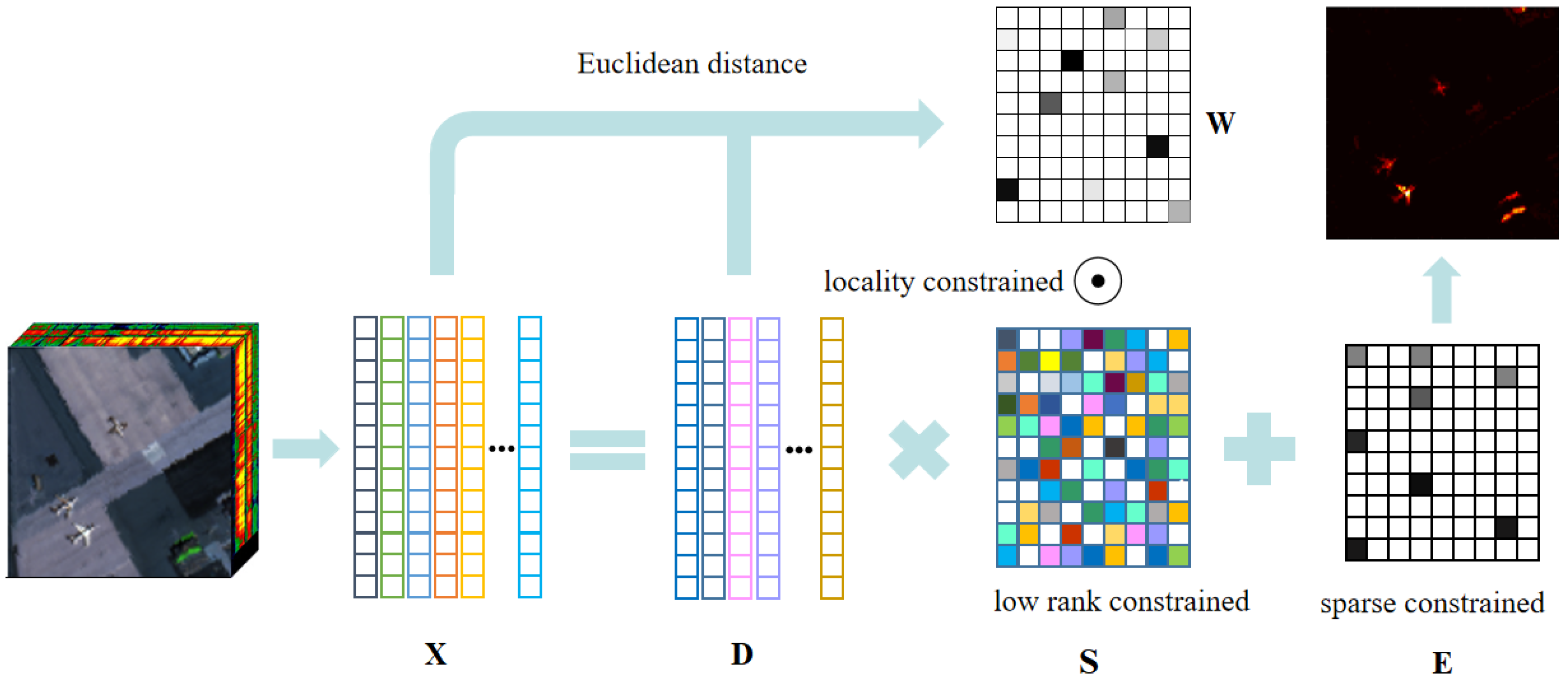
The remainder of this paper is organized as follows. The detailed description of our algorithm is presented in Section 2. The experimental details and analyses are shown in Section 3. The conclusions are given in Section 4.

2. Proposed Method

2.1. LRR for Hyperspectral Anomaly Detection

There is high spectral correlation and spatial homogeneity among background pixels [5] in a HSI, and the background pixel is assumed to be sampled from a union of multiple low-dimensional subspace. This makes the background part of the low-rank characteristic. The anomalies have low occurrence probability and small proportion, which makes them sparse. Suppose that an HSI is denoted as $\mathbf{I}\in {\mathbb{R}}^{w\times h\times p}$. Generally, the $\mathbf{I}$ is concerted to a 2D matrix $\mathbf{X}={\left\{{\mathbf{x}}_i\right\}}_{i=1}^n\in {\mathbb{R}}^{n\times p}$, where $n=w\times h$ is the number of pixels and p is number of spectral bands. The low rank representation (LRR) model [29] proposed by Liu et al. is developed to recover the subspace structures of a matrix, and usually used to decompose a matrix into a low rank part and a residual part. Based on low rank representation (LRR) model [29], $\mathbf{X}$ can be decomposed into the background and anomaly part, which is formulated as

$$\begin{array}{cc}\hfill \underset{\mathbf{S},\mathbf{E}}{min}& \mathrm{rank}\left(\mathbf{S}\right)+{\lambda \parallel \mathbf{E}\parallel }_0\hfill \\ \hfill \mathrm{s}.\mathrm{t}& \mathbf{X}=\mathbf{DS}+\mathbf{E}\hfill \end{array}$$

(1)

where $\mathbf{DS}$ denotes the background part, which can be expressed as the product of a background dictionary $\mathbf{D}$ and corresponding representation coefficient matrix $\mathbf{S}$. The dictionary $\mathbf{D}=[{\mathbf{d}}_1,{\mathbf{d}}_2,\cdots ,{\mathbf{d}}_m]$ is composed of representative background pixels. The matrix $\mathbf{E}$ is the residual matrix referring to the anomaly part. ${\parallel \mathbf{E}\parallel }_0$ is $l_0$ norm of $\mathbf{E}$, which is the number of nonzero atoms in $\mathbf{E}$.

However, the rank function and $l_0$ norm are discrete and non-convex. The problem (1) is NP-hard. Fortunately, the $l_1$ norm is the optimal convex approximation of $l_0$ norm, and the nuclear norm is an appropriate surrogate to rank function [29]. The problem (1) is rewritten as follows,

$$\begin{array}{cc}\hfill \underset{\mathbf{S},\mathbf{E}}{min}& {\parallel \mathbf{S}\parallel }_{*}+\lambda {\parallel \mathbf{E}\parallel }_1\hfill \\ \hfill \mathrm{s}.\mathrm{t}& \mathbf{X}=\mathbf{DS}+\mathbf{E}\hfill \end{array}$$

(2)

where ${\parallel \mathbf{S}\parallel }_{*}$ is the nuclear norm of $\mathbf{S}$, which is the sum of singular values of $\mathbf{S}$. ${\parallel \mathbf{E}\parallel }_1$ is the $l_1$ norm of $\mathbf{E}$, which is the sum of absolute value of all elements in $\mathbf{E}$. The problem (2) and problem (1) are equivalent when noise is free [29]. Real HSIs contain lots of noises; therefore, a robust model is formulated as

$$\begin{array}{cc}\hfill \underset{\mathbf{S},\mathbf{E}}{min}& {\parallel \mathbf{S}\parallel }_{*}+\lambda {\parallel \mathbf{E}\parallel }_{2,1}\hfill \\ \hfill \mathrm{s}.\mathrm{t}& \mathbf{X}=\mathbf{DS}+\mathbf{E}\hfill \end{array}$$

(3)

where ${\parallel \mathbf{E}\parallel }_{2,1}$ is the sum of the $l_2$ norm of each column of matrix $\mathbf{E}$. Compared to $l_0$ norm, $l_{2,1}$ norm can force more columns of $\mathbf{E}$ to be zero vector. $\lambda$ is a regularization parameter, which balances the weights of low-rank and sparsity characteristic.

The problem (3) can be solved by the Inexact Augmented Lagrange Multiplier (IALM) [32,33] algorithm. Once the decomposition process is completed, the residual matrix $\mathbf{E}$ is utilized to get the final detection map. The anomaly degree $G\left({\mathbf{x}}_i\right)$ is defined as the $l_2$ norm of the ith column of matrix $\mathbf{E}$.

$$G\left({\mathbf{x}}_i\right)={∥{\left[\mathbf{E}\right]}_{:,i}∥}_2$$

(4)

If $G\left({\mathbf{x}}_i\right)$ is larger than a given threshold, the pixel ${\mathbf{x}}_i$ will be regarded as an anomaly pixel. Moreover, the $G\left({\mathbf{x}}_i\right),i=1,2,\cdots ,n$ is reshaped to the spatial size of $\mathbf{I}$, yielding the detection map $\mathbf{G}$.

2.2. Locality Constrained LRR

The pixel in a local region belong to similar materials with high probability, and their spectrum vector are similar. It is beneficial for HAD task to explore the local similarity, whose importance has been shown in many articles [34,35]. However, the LRR is a global structure model, which inevitably neglects local geometrical information [29]. Manifold learning is an important dimensionality reduction method, which attempts to obtain the intrinsic distribution and geometry structure of high-dimensional data. Multi-dimensional scaling (MDS) [36] is a classical manifold learning algorithm, which keeps the geometrical structure of original data via holding the distances among points. Motivated by this, we adopt the distance weight $W_{ij}={\parallel {\mathbf{x}}_i-{\mathbf{x}}_j\parallel }_2^2\in \mathbf{W}$, i.e., the Euclidean distance between any two points, to constrain the representation coefficient $\mathbf{S}$, in order to make the pixels who are close in original space have similar coefficients in representation space $\mathbf{S}$.

As in [37,38], We utilize the following term to preserve the local geometrical structure in the process of low rank decomposition.

$$\mathbf{W}\odot \mathbf{S}$$

(5)

where ⊙ is the Hadamard product which is the element-wise product of two matrix. If two pixels are close in a HSI, the weight $W_{ij}$ with small value can make the corresponding pixels in representation space as close as possible.

In the HAD task, most pixels belong to the background, and they are composed of a few main materials. Pixels in a HSI can be sparsely represented by few nonzero coefficients with a dictionary. Therefore, the matrix $\mathbf{S}$ is also sparse, not only low-rank. We use the following term to characterize this.

$${\parallel \mathbf{W}\odot \mathbf{S}\parallel }_1$$

(6)

where ${\parallel \mathbf{W}\odot \mathbf{S}\parallel }_1$ can be seen as the $l_1$ norm of matrix $\mathbf{S}$ weighted by $\mathbf{W}$, which can encourage the sparsity of $\mathbf{W}\odot \mathbf{S}$.

Subsequently, the newly introduced locality constrained term is added into the original objective function (3) of LRR, which is expressed as,

$$\begin{array}{cc}\hfill \underset{\mathbf{S},\mathbf{E}}{min}& {\parallel \mathbf{S}\parallel }_{*}+{\lambda \parallel \mathbf{E}\parallel }_{2,1}+\alpha {\parallel \mathbf{W}\odot \mathbf{S}\parallel }_1\hfill \\ \hfill \mathrm{s}.\mathrm{t}& \mathbf{X}=\mathbf{DS}+\mathbf{E}\hfill \end{array}$$

(7)

where $\alpha$ is a locality constrained regularization parameter.

2.3. Active Dictionary Learning for LRR

For the anomaly detectors based on LRR model, the dictionary construction is of great importance. However, most HAD methods with LRR model need to construct dictionary in advance, that is to say, they have multiple steps. For example, in [26,27,39], the dictionary is built through a clustering algorithm independently. Since there is no prior information about the number of background materials, the number of clusters is difficult to determine, resulting in a big problem of dictionary construction. Different from previous methods, we attempt to learn a compact and discriminative dictionary by exploiting the local geometrical information. Thus, the dictionary learning is integrated into the optimization process of problem (7), in order to learn the representation coefficient $\mathbf{S}$ and dictionary $\mathbf{D}$ simultaneously. The objective function is formulated as follows,

$$\begin{array}{cc}\hfill \underset{\mathbf{S},\mathbf{E}}{min}& {\parallel \mathbf{S}\parallel }_{*}+{\lambda \parallel \mathbf{E}\parallel }_{2,1}{+\alpha \parallel \mathbf{W}\odot \mathbf{S}\parallel }_1+\frac{\gamma }{2}{\parallel \mathbf{D}\parallel }_F^2\hfill \\ \hfill \mathrm{s}.\mathrm{t}& \mathbf{X}=\mathbf{DS}+\mathbf{E}\hfill \end{array}$$

(8)

where ${\parallel \mathbf{D}\parallel }_F^2$ is the Frobenius norm of $\mathbf{D}$, aiming to avoid scale change, $\gamma$ is a balance parameter. The optimization process of problem (8) is introduced briefly in Section 2.4. For our HAD method based on the LCLRR model, the procedure is summarized in Algorithm 1, and the flowchart is shown in Figure 1.

Algorithm 1 HAD algorithm based on LCLRR model.

Input:    Hyperspectral image $\mathbf{X}$; Regularization parameter $\lambda$, $\alpha$, and $\gamma$; Number of atoms K in dictionary $\mathbf{D}$; Output:    Anomaly detection map $\mathbf{G}$. 1: Randomly select K pixels to form the initial dictionary $\mathbf{D}$. 2: Compute the Euclidean distance between $\mathbf{D}$ and $\mathbf{X}$ to form the weight matrix $\mathbf{W}$. 3: Optimize the problem (8) with the Algorithm 2 to obtain the residual matrix $\mathbf{E}$. 4: Obtain the detection map as Equation (4).

2.4. Optimization Procedure of LCLRR

To make the objective function separable for problem (8), two auxiliary variables $\mathbf{P}$ and $\mathbf{Q}$ are introduced. The original problem is rewritten as follows,

$$\begin{array}{cc}\hfill \underset{\mathbf{S},\mathbf{P},\mathbf{Q},\mathbf{E},\mathbf{D}}{min}& {\parallel \mathbf{P}\parallel }_{*}+{\lambda \parallel \mathbf{E}\parallel }_{2,1}{+\alpha \parallel \mathbf{W}\odot \mathbf{Q}\parallel }_1+\frac{\gamma }{2}{\parallel \mathbf{D}\parallel }_F^2\hfill \\ \hfill \mathrm{s}.\mathrm{t}& \mathbf{X}=\mathbf{DS}+\mathbf{E},\mathbf{S}=\mathbf{P},\mathbf{S}=\mathbf{Q}\hfill \end{array}$$

(9)

This constrained optimization problem (9) can be solved by the IALM algorithm [32,37]. The augmented Lagrangian function of Equation (9) is as follows,

$$\begin{array}{cc}\hfill & \mathcal{L}\left(\mathbf{S},\mathbf{P},\mathbf{Q},\mathbf{E},\mathbf{D},{\mathbf{Y}}_1,{\mathbf{Y}}_2,{\mathbf{Y}}_3,\mu \right)\hfill \\ \hfill & ={\parallel \mathbf{P}\parallel }_{*}+{\lambda \parallel \mathbf{E}\parallel }_{2,1}{+\alpha \parallel \mathbf{W}\odot \mathbf{Q}\parallel }_1+\frac{\gamma }{2}{\parallel \mathbf{D}\parallel }_F^2+〈{\mathbf{Y}}_1,\mathbf{X}-\mathbf{D}\mathbf{S}-\mathbf{E}〉\hfill \\ \hfill & +\langle {\mathbf{Y}}_2,\mathbf{S}-\mathbf{P}\rangle +\langle {\mathbf{Y}}_3,\mathbf{S}-\mathbf{Q}\rangle +\frac{\mu }{2}\left({\parallel \mathbf{X}-\mathbf{D}\mathbf{S}-\mathbf{E}\parallel }_F^2{+\parallel \mathbf{S}-\mathbf{P}\parallel }_F^2+{\parallel \mathbf{S}-\mathbf{Q}\parallel }_F^2\right)\hfill \end{array}$$

(10)

where ${\mathbf{Y}}_1,{\mathbf{Y}}_2,{\mathbf{Y}}_3$ are Lagrange multipliers, $\mu$ is a positive penalty coefficient. $\langle \mathbf{A},\mathbf{B}\rangle$ is trace of ${\mathbf{A}}^T\mathbf{B}$. The problem (10) has multiple variables, it can be solved iteratively by updating one variable with others fixed [27,37]. The processing procedure can be broken down into several steps.

Step 1: updating $\mathbf{S}$ with other variables fixed, the problem can be formulated as follows,

$$\begin{array}{cc}\hfill & {\mathbf{S}}^{k+1}=arg\underset{\mathbf{S}}{min}<{\mathbf{Y}}_1^k,\mathbf{X}-{\mathbf{D}}^k\mathbf{S}-{\mathbf{E}}^k>\hfill \\ \hfill & +<{\mathbf{Y}}_2^k,\mathbf{S}-{\mathbf{J}}^{k+1}>+<{\mathbf{Y}}_3^k,\mathbf{S}-{\mathbf{L}}^k>\hfill \\ \hfill & +\frac{{\mu }^k}{2}\left({∥\mathbf{X}-{\mathbf{D}}^k\mathbf{S}-{\mathbf{E}}^k∥}_F^2+{∥\mathbf{S}-{\mathbf{J}}^{k+1}∥}_F^2+{∥\mathbf{S}-{\mathbf{L}}^k∥}_F^2\right)\hfill \end{array}$$

(11)

Step 2: updating $\mathbf{P}$ with other variables fixed, the problem can be formulated as follows,

$$\begin{array}{cc}\hfill & {\mathbf{P}}^{k+1}=arg\underset{\mathbf{P}}{min}{\parallel \mathbf{P}\parallel }_{*}+<{\mathbf{Y}}_2^k,{\mathbf{S}}^k-\mathbf{P}>+\frac{{\mu }^k}{2}{∥{\mathbf{S}}^k-\mathbf{P}∥}_F^2\hfill \\ \hfill & =arg\underset{\mathbf{P}}{min}\frac{1}{{\mu }^k}{\parallel \mathbf{P}\parallel }_{*}+\frac{1}{2}{∥\mathbf{P}-\left({\mathbf{S}}^k+\frac{{\mathbf{Y}}_2^k}{{\mu }^k}\right)∥}_F^2\hfill \end{array}$$

(12)

Step 3: updating $\mathbf{Q}$ with other variables fixed, the problem can be formulated as follows,

$$\begin{array}{cc}\hfill & {\mathbf{Q}}^{k+1}=arg\underset{\mathbf{L}}{min}\alpha {\parallel \mathbf{W}\odot \mathbf{Q}\parallel }_1+<{\mathbf{Y}}_3^k,{\mathbf{S}}^{k+1}-\mathbf{Q}>\hfill \\ \hfill & +\frac{{\mu }^k}{2}{∥{\mathbf{S}}^{k+1}-\mathbf{Q}∥}_F^2\hfill \\ \hfill & =arg\underset{\mathbf{Q}}{min}\alpha {\parallel \mathbf{W}\odot \mathbf{L}\parallel }_1+\frac{{\mu }^k}{2}{∥\mathbf{Q}-\left({\mathbf{S}}^{k+1}+\frac{{\mathbf{Y}}_3^k}{{\mu }^k}\right)∥}_F^2\hfill \end{array}$$

(13)

Step 4: updating $\mathbf{E}$ with other variables fixed, the problem can be formulated as follows,

$$\begin{array}{cc}\hfill & {\mathbf{E}}^{k+1}=arg\underset{\mathbf{E}}{min}\lambda {\parallel \mathbf{E}\parallel }_{21}+<{\mathbf{Y}}_1^k,\mathbf{X}-{\mathbf{D}}^k{\mathbf{S}}^{k+1}-\mathbf{E}>\hfill \\ \hfill & +\frac{{\mu }^k}{2}{∥\mathbf{X}-{\mathbf{D}}^k{\mathbf{S}}^{k+1}-\mathbf{E}∥}_F^2\hfill \\ \hfill & =arg\underset{\mathbf{E}}{min}\frac{\lambda }{{\mu }^k}{\parallel \mathbf{E}\parallel }_{21}+\frac{1}{2}{∥\mathbf{E}-\left(\mathbf{X}-{\mathbf{D}}^k{\mathbf{S}}^{k+1}+\frac{{\mathbf{Y}}_1^k}{{\mu }^k}\right)∥}_F^2\hfill \end{array}$$

(14)

Step 5: updating $\mathbf{D}$ with other fixed variables, the problem can be formulated as follows,

$$\begin{array}{cc}\hfill & {\mathbf{D}}^{k+1}=arg\underset{\mathbf{D}}{min}\frac{\gamma }{2}{\parallel \mathbf{D}\parallel }_F^2+<{\mathbf{Y}}_1,\mathbf{X}-\mathbf{D}{\mathbf{S}}^{k+1}-{\mathbf{E}}^{k+1}>\hfill \\ \hfill & +\frac{{\mu }^k}{2}{∥\mathbf{X}-\mathbf{D}{\mathbf{S}}^{k+1}-{\mathbf{E}}^{k+1}∥}_F^2\hfill \\ \hfill & =\left[\frac{{\mathbf{Y}}_1^k{\left({\mathbf{S}}^{k+1}\right)}^T}{{\mu }^k}-\left({\mathbf{E}}^{k+1}-\mathbf{X}\right){\left({\mathbf{S}}^{k+1}\right)}^T\right]{\left(\frac{\gamma }{{\mu }^k}\mathbf{I}+{\mathbf{S}}^{k+1}{\left({\mathbf{S}}^{k+1}\right)}^T\right)}^{-1}\hfill \end{array}$$

(15)

The whole optimization process is summarize in Algorithm 2.

Algorithm 2 The optimization of problem (10) by the IALM algorithm.

Input:    Input matrix $\mathbf{X}$; Regularization parameter $\lambda$, $\alpha$, and $\gamma$; Weight matrix $\mathbf{W}$; Output:    Representation coefficient matrix $\mathbf{S}$; Dictionary matrix $\mathbf{D}$; Residual matrix $\mathbf{E}$; 1: Initialize ${\mathbf{S}}^0=0$, ${\mathbf{P}}^0=0$, ${\mathbf{Q}}^0=0$, ${\mathbf{E}}^0=0$, ${\mathbf{Y}}_1^0=0$, ${\mathbf{Y}}_2^0=0$, ${\mathbf{Y}}_3^0=0$, ${\mu }_{max}={10}^8$, $ϵ={10}^{}-6$, $\rho =1.15$. 2: while${∥{\mathbf{S}}^{k+1}-{\mathbf{P}}^{k+1}∥}_{\infty }<\epsilon ,{∥{\mathbf{S}}^{k+1}-{\mathbf{Q}}^{k+1}∥}_{\infty }<\epsilon$ and $\mathbf{X}-{\mathbf{D}}^{k+1}{\mathbf{S}}^{k+1}-{\mathbf{E}}^{k+1}{\parallel }_{\infty }<\epsilon$ do 3: Update the $\mathbf{S}$, $\mathbf{P}$, $\mathbf{Q}$, $\mathbf{E}$, $\mathbf{D}$ as the procedure in Section 2.4. 4: Update the Lagrangian multiplier ${\mathbf{Y}}_1$, ${\mathbf{Y}}_2$, ${\mathbf{Y}}_3$: ${\mathbf{Y}}_1^{k+1}={\mathbf{Y}}_1^k+{\mu }^k\left(\mathbf{X}-{\mathbf{D}}^{k+1}{\mathbf{S}}^{k+1}-{\mathbf{E}}^{k+1}\right)$ ${\mathbf{Y}}_2^{k+1}={\mathbf{Y}}_2^k+{\mu }^k\left({\mathbf{S}}^{k+1}-{\mathbf{P}}^{k+1}\right)$ ${\mathbf{Y}}_3^{k+1}={\mathbf{Y}}_3^k+{\mu }^k\left({\mathbf{S}}^{k+1}-{\mathbf{Q}}^{k+1}\right)$ 5: Update $\mu$: ${\mu }^{k+1}=min\left({\mu }_{max},\rho {\mu }^k\right)$ 6: do while

3. Experiments and Result Analysis

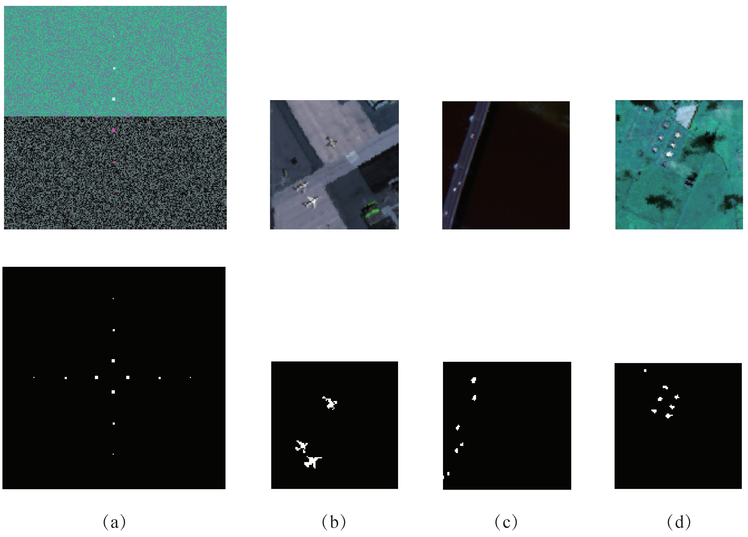
3.1. HSI Dataset

One simulated dataset and three real hyperspectral datasets are used to evaluate our method’s performance. The first is a simulated dataset [40]. It has the spatial size of $200\times 200$ and 105 spectral bands. The background materials are mixed by five plants in random proportions. The plants are lawn grass, dry long grass, black shrub leaf, sage brush, and tumbleweed, whose spectral vectors can be downloaded from the U.S. Geological Survey vegetation spectral library. The anomalies are set to pure materials. There are 12 anomaly objects with the size of $1\times 1$, $2\times 2$, and $3\times 3$ implanted into the complicated background in the shape of a cross. The pseudo-color image and its corresponding reference map are shown in Figure 2a.

The second is the San Diego airport dataset, which was captured by the Airborne Visible/Infrared Imaging Spectrometer (AVIRIS) in San Diego, CA, USA. The whole size of the image is $400\times 400$, and its spatial resolution is 3.5 m. After removing water absorption, low SNR, and poor-quality bands, there are 189 spectral bands remained in wavelength ranging from 370 to 2510 nm. In general, a sub-image of $100\times 100$ in the top-left is chosen as the test image. The background scene mainly containing hangars, airstrips, and meadows, is complicated. Three airplanes consisting of 57 pixels are taken as anomaly objects. The pseudo-color image and its corresponding reference map are shown in Figure 2b.

The third is the Pavia center dataset, which was captured by the Reflective Optics System Imaging Spectrometer (ROSIS) over a urban center in Pavia, Italy. This dataset have the size of $108\times 120$, and 1.3 m spatial resolution. There are 102 spectral bands in wavelength ranging from 430 to 860 nm. The background scene mainly includes a bridge and river. Six vehicles on the bridge are regarded as the anomaly objects. The pseudo-color image and its corresponding reference map are displayed in Figure 2c.

The fourth is the Texas Coast urban dataset, which was also captured by the AVIRIS sensor in Texas Coast. The size of the image is $100\times 100$, and its spatial resolution is 17.2 m. There are 204 spectral bands ranging from 450 to 1350 nm. The background scene comprises a stretch of meadow and some groves. The houses are regarded as anomaly objects. This image, it should be noted, is contaminated by some serious strip noises; hence, it is a challenging task to recognize all anomaly pixels with noise suppression. The pseudo-color image and its corresponding reference map are shown in Figure 2d.

3.2. Comparison Algorithm and Evaluation Metrics

Seven typical algorithms are compared with our proposed LCLRR algorithm. These competitors include the global RX (GRX) [12], local RX (LRX) [12], CRD [21], BJSR [19], LSMAD [25], LRASR [27], and KIFD [41]. The GRX and LRX are statistical model-based methods. The BJSR, CRD, LSMAD, and LRASR are representation-based methods, they use the SR, CR, and LRR model, respectively. The KIFD is based on the isolation forest theory [42], which isolates anomaly pixels from background directly.

To evaluate the results of different algorithms intuitively, our experiments employ the following three metrics: the receiver operating characteristic (ROC) curve [43], the area under the ROC curve (AUC), and the box plot [44]. The ROC curve illustrate the relationship between detection probability ($DP$) and false alarm rate ($FAR$), who are computed as:

$$DP=\frac{N_D}{N_T},FAR=\frac{N_F}{N_B},$$

(16)

where $N_D$ denotes the number of anomaly pixels detected correctly, $N_T$ is the number of anomaly pixels as the reference map shows, $N_F$ indicates the number of misidentified anomaly pixels, which are the background pixels actually. $N_B$ is the number of background pixels. When the $FAR$ is constant, the algorithm with larger $DP$ gets better performance. In other words, the algorithm whose ROC curve is closer to the top-left corner performs better. The AUC value is a quantitative evaluation metric. The algorithm with larger AUC value gets a better detection performance.

The box plot is used to visualize anomaly–background separability. Usually in a box plot, the red color box describes the distribution of anomaly pixels, and the blue color box represents the background distribution. The middle line in each box is the average value of their corresponding pixels. The larger the gap between the anomaly and background boxes is, the higher the anomaly-background separation degree will be. And the shorter the background box is, the more background information the algorithm suppresses.

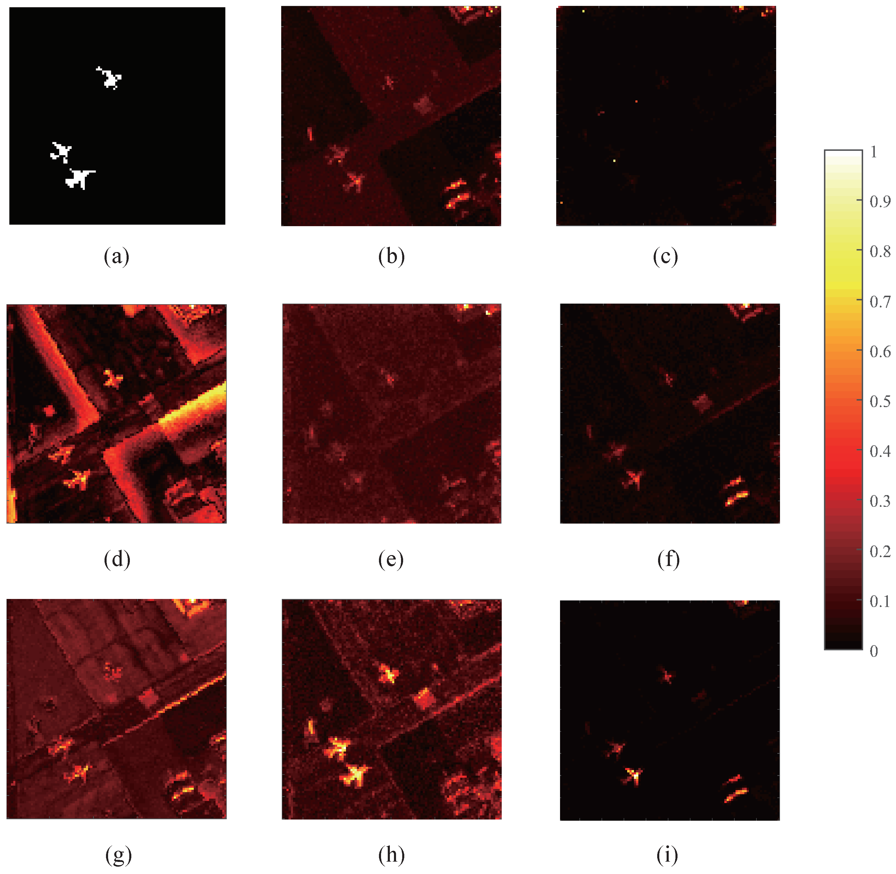
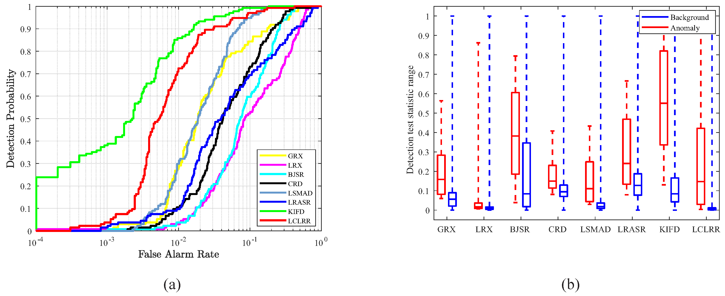
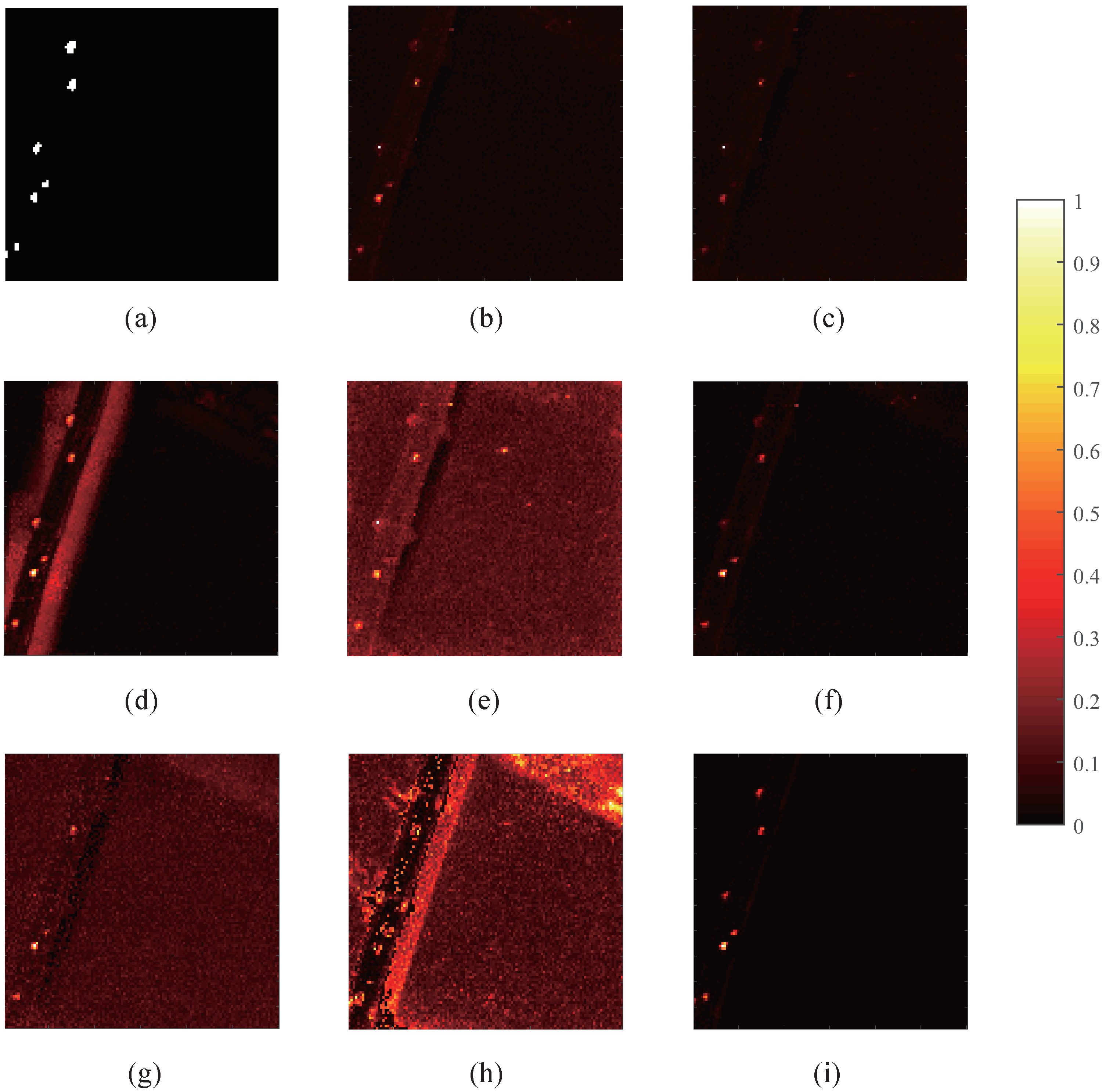
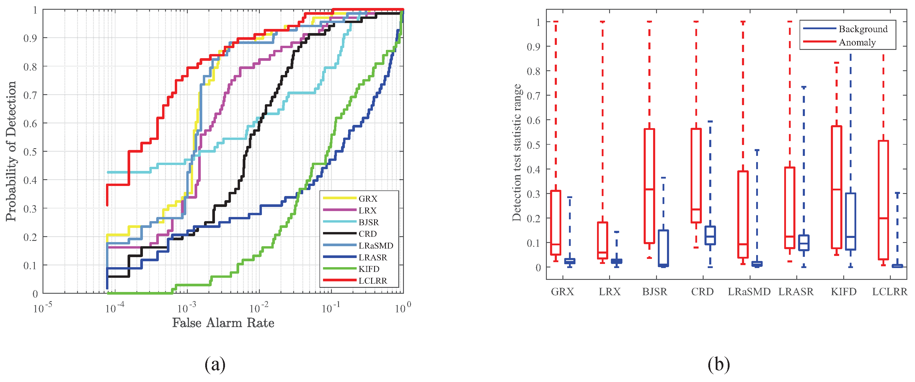
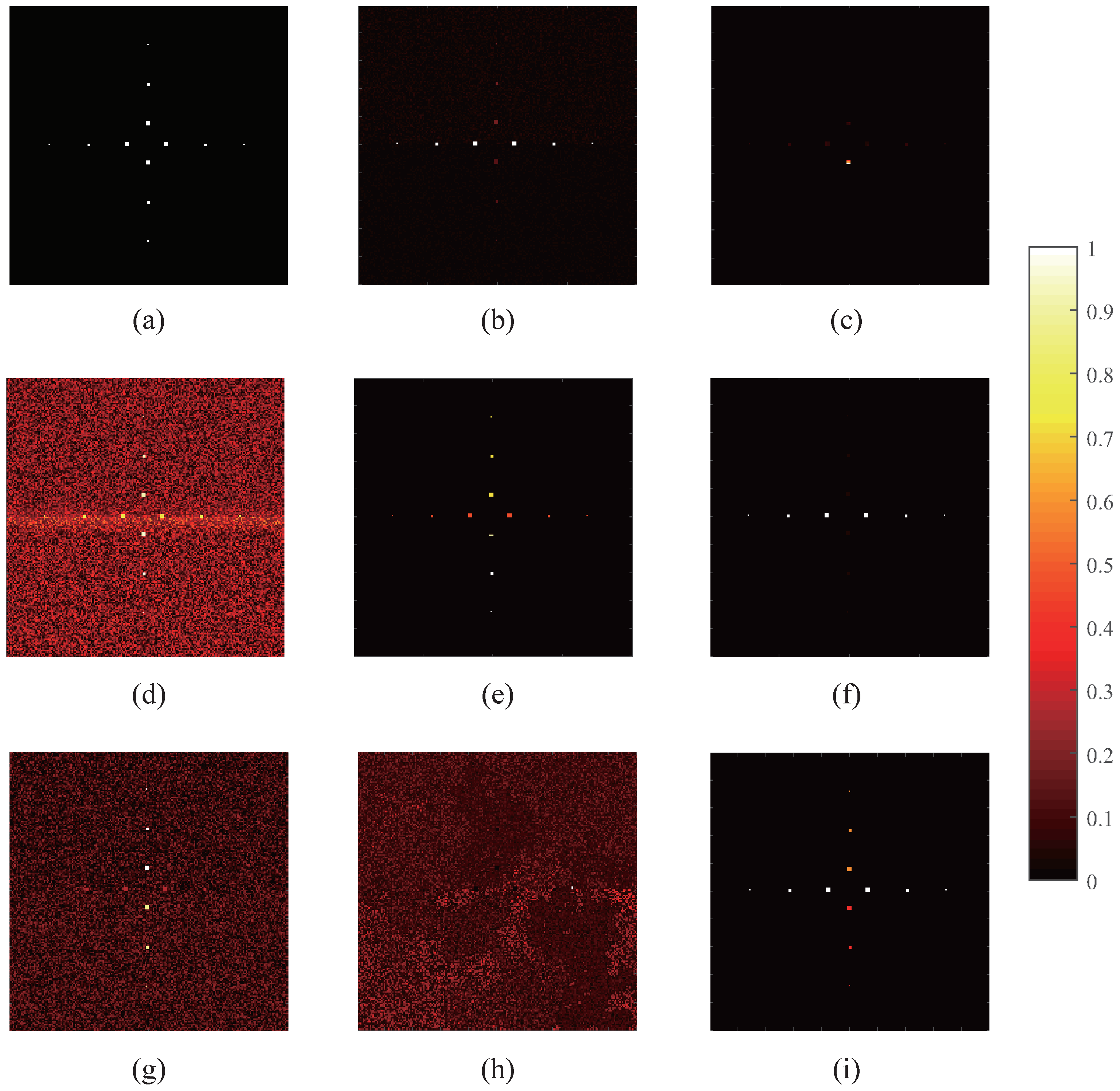
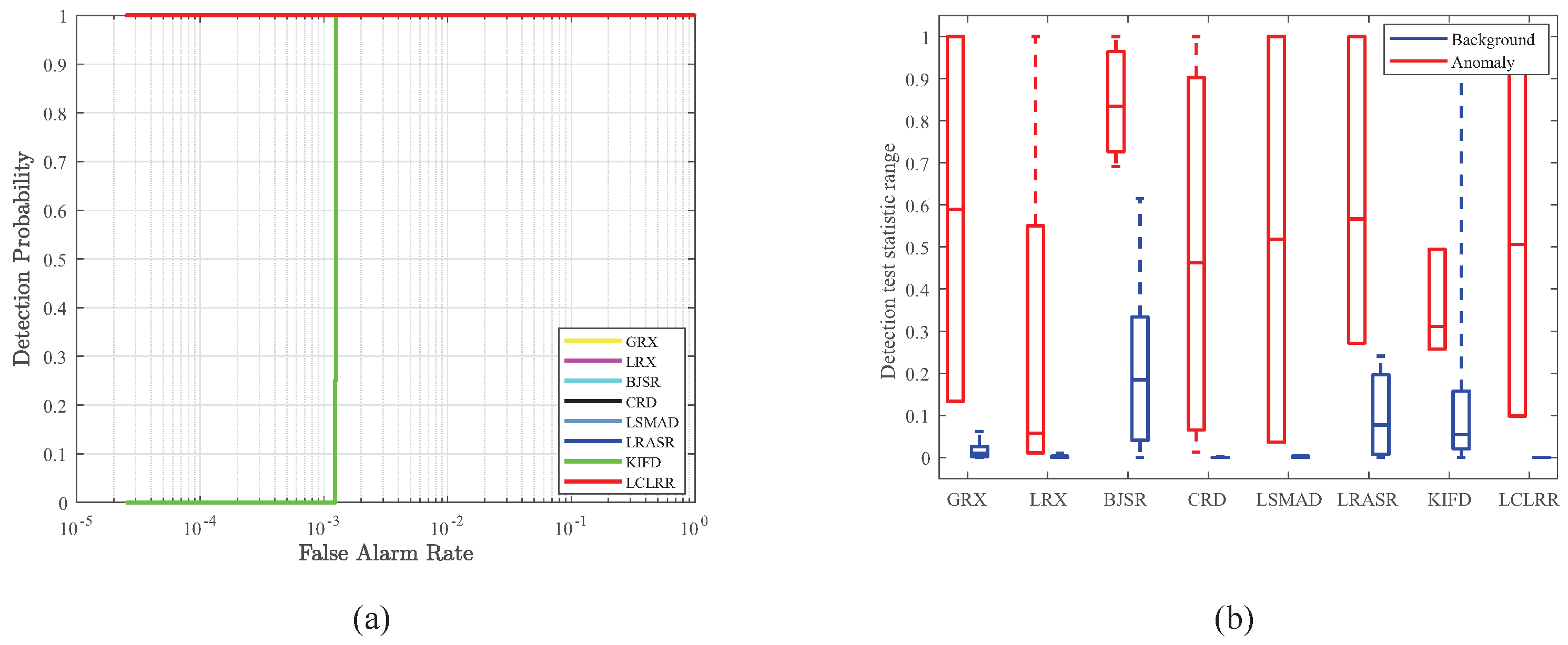
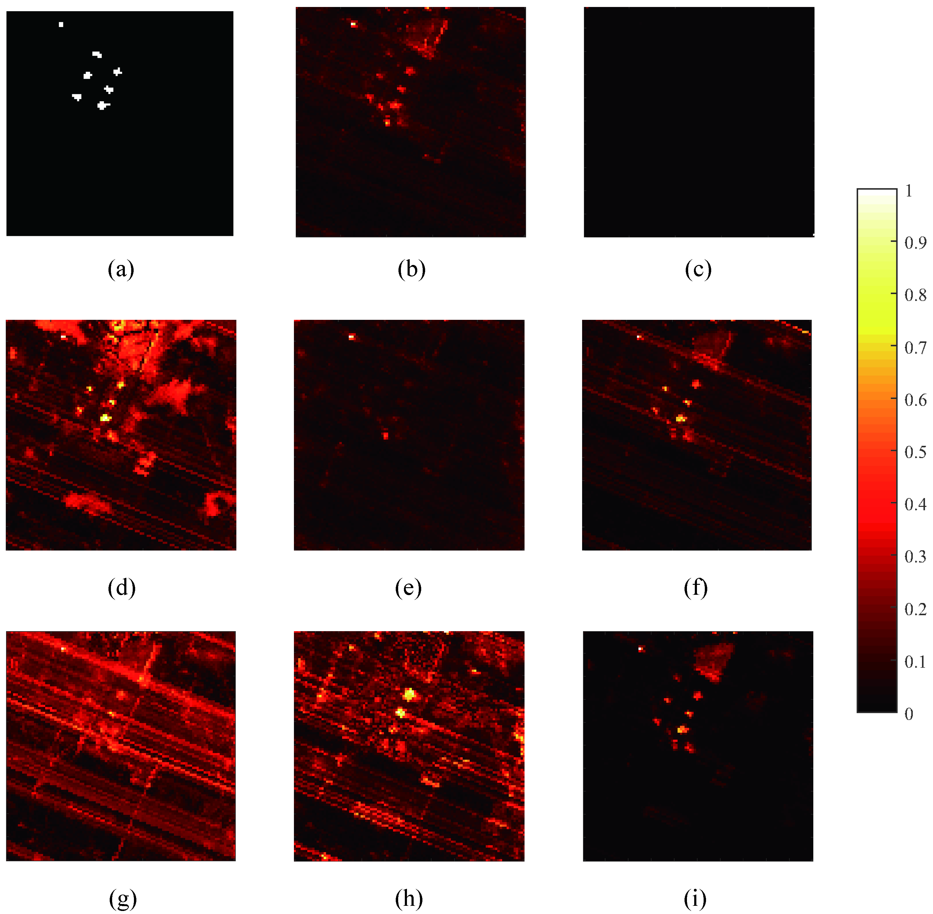
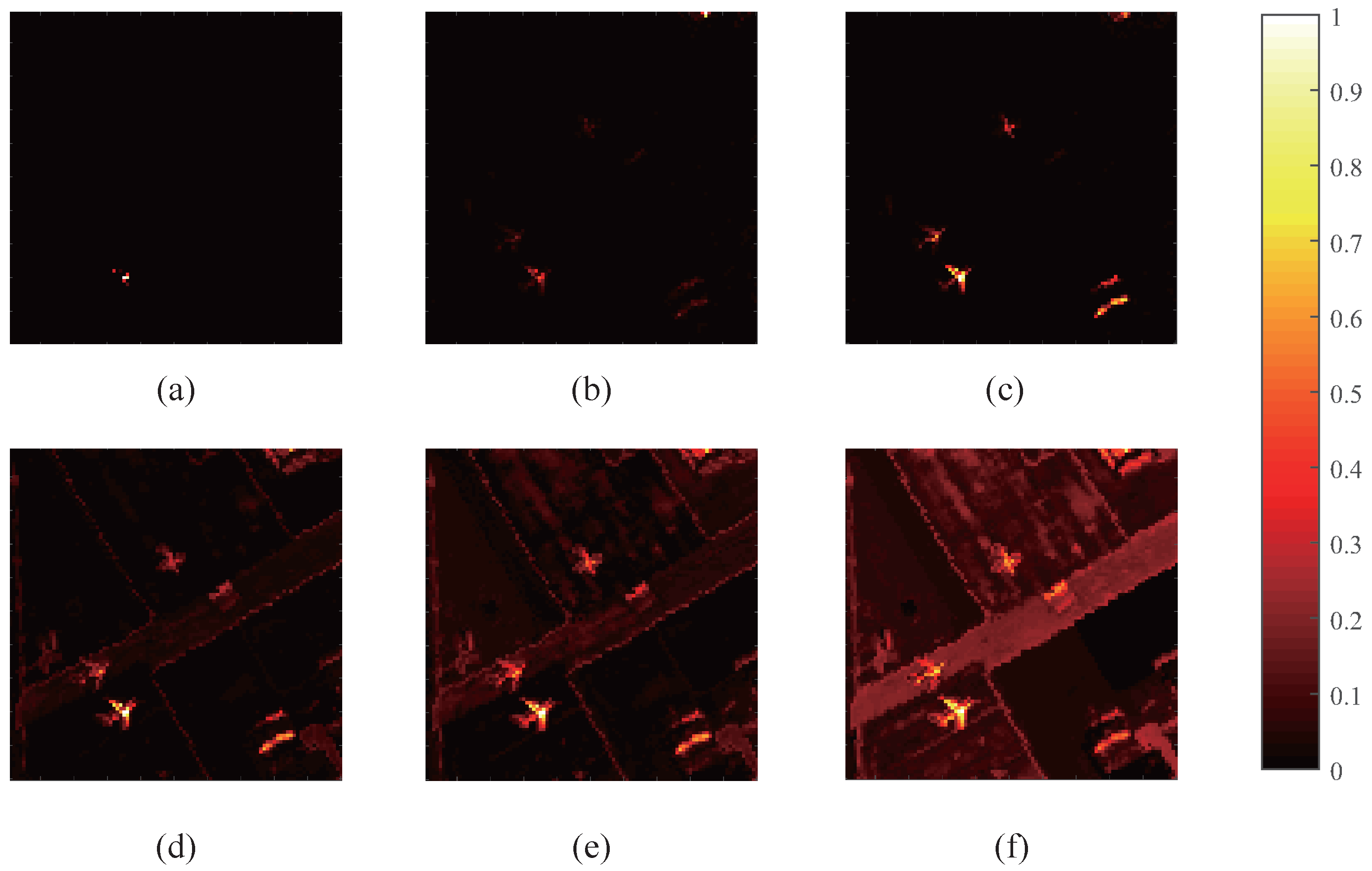
3.3. Detection Performance

For the comparison algorithms, there are some parameter settings to be declared in advance. The detection performances of the LRX, BJSR, and CRD methods are closely associated with the double-window size $\{W_{outer},W_{inner}\}$. To sort out the best result, $\{W_{outer},W_{inner}\}$ is set to $\{3,23\}$, $\{3,25\}$, $\{3,29\}$, $\{5,23\}$, $\{5,25\}$, and $\{3,29\}$ in turn. Moreover, the regularization parameter is set to $0.1$ for the CRD method. For the LSMAD method, the rank is set to 28, the cardinality is set to $0.02\times p$ (p is number of spectral bands). For the LRASR method, the parameter $\beta$ is set to $0.01$, the parameter $\lambda$ is set to 1, the number of clusters are set to 15, the number of pixels in each background cluster is set to 20. For the KIFD method, the dimension parameter $\zeta$, the number of isolation trees q, and the size of train dataset M are set to 300, 1000, and $3\%\times n$ (n is the number of pixels), respectively.

For our method, there are four parameters involved in the experiments. They are the sparsity regularization parameter $\lambda$, the locality regularization parameter $\alpha$, the dictionary regularization parameter $\gamma$, and the number of atoms K in dictionary $\mathbf{D}$. The influence of those parameters on the detection performance will be discussed in Section 3.4 in detail. Here, we just give the optimal parameter settings in following experiments. For the simulated dataset, several parameter combinations can make our method acquire the AUC value of 1. For example, the $\lambda ,\alpha ,\gamma$ are set to $0.1,0.05,0.05$. For the San Diego airport dataset, the $\lambda ,\alpha ,\gamma$ are set to $0.5,0.1,0.05$. For the Pavia center dataset, the $\lambda ,\alpha ,\gamma$ are set to $0.5,0.3,0.05$. For the Texas Coast urban dataset, the $\lambda ,\alpha ,\gamma$ are set to $0.1,0.01,0.05$. For all datasets, the number of atoms K is set to 300, considering the performance and efficiency comprehensively.

For the simulated dataset, the detection maps are displayed in Figure 3. We can find that our method and CRD method can detect all anomaly pixels with excellent results of background suppression. For the GRX, LRX, and LSMAD method, the background information is suppressed effectively, but only some anomaly objects are identified clearly. For the BJSR and LRASR method, the detection map is blurry. It is obvious that the effect of background suppression is bad. For the KIFD method, few anomaly pixels are detected. It performs poorly in both anomaly detection and background suppression. The ROC curves of different algorithms are displayed in Figure 4a. The curves of all algorithms except the KIFD are at the line whose y-coordinate is 1. The AUC values are listed in

Table 1. The AUC values of different algorithms for four datasets including simulated, San Diego airport, Pavia center, and Texas Coast urban. The best results are in bold, and the second-best outcomes are underlined.

Methods	Simulated	San Diego Airport	Pavia Center	Texas Coast Urban
GRX [12]	1	0.9403	0.9901	0.9907
LRX [12]	1	0.8173 (5,29 )	0.9734 (5,29)	0.9124 (5,29)
BJSR [19]	1	0.8844 (3,23)	0.9579 (5,23)	0.9200 (5,23)
CRD [21]	1	0.9159 (5,23)	0.9623 (5,29)	0.9421 (5,23)
LSMAD [25]	1	0.9666	0.9877	0.9833
LRASR [27]	1	0.8661	0.7148	0.9425
KIFD [41]	0.9988	0.9919	0.7707	0.9178
LCLRR	1	0.9846	0.9957	0.9944

, all algorithms except the KIFD method have the AUC values of 1. Obviously, the ROC curve and AUC value are unable to distinguish the performance difference of comparison algorithms. Here, the box plot depicted in Figure 4b can tell us more. The gap between the background and anomaly boxes for our method is the largest, which demonstrates that our method has the highest anomaly-background separation degree. Moreover, the background box of our method is shorter, which indicates that our method has good background suppression ability.

For the San Diego airport dataset, the detection maps are displayed in Figure 5. It can be observed intuitively that the GRX, LSMAD, KIFD, and our method get better performance. For the LRX method, a small number of anomaly pixels are detected, although the background is suppressed effectively. For the BJSR method, the anomaly-background separation degree is low, resulting in a blurred boundary between the background and anomalies. It is also proved in the box plot in Figure 6b, where the background box and anomaly box of the BJSR method is overlapped. For the KIFD method, it has a higher detection probability, and anomaly objects are clear. The ROC curves of different algorithms are shown in Figure 6a. The ROC curve of the KIFD method is the closest, indicating it has the best performance. The AUC values are listed in the second column of Table 1. The KIFD method have the largest AUC value, and our method is the second best. The box plot is shown in Figure 6b. The gap between these boxes for KIFD method is the largest, nevertheless, its anomaly box is large. This indicates that the KIFD method does not suppress the background well. On the contrary, our method performs well in suppressing the background information, because its background box is the shortest.

For the Pavia center dataset, the detection maps are shown in Figure 7. It can be founded that our proposed method performs best among all competitors. Our method can not only detect all anomaly pixels accurately, but also suppress the background information thoroughly, especially the edge of bridge. For the GRX, LRX, and LSMAD method, most of anomaly pixels have been detected, but some are not clear enough. The BJSR method can locate anomaly objects, but fail to suppress the edge of bridge, leading to high $FAR$. The CRD and LRASR method can not set a clear boundary to separate the background and anomaly part. The KIFD method performs poorly. It can not locate anomaly objects and suppress background information. The ROC curves of different algorithms are displayed in Figure 8a. The curve of our method is the closest to the top-left corner, indicating that our method is the best. The results of AUC value are shown in Table 1. The AUC value of our method is 0.9957, which is the largest of all. The box plots are shown in Figure 8b, which give us more details than other two metrics. For the BJSR, LRASR, and KIFD methods, the anomaly box and background box overlapped, indicating low anomaly-background separation degree. This is also verified mutually in the detection maps in Figure 7. For our method, there is a certain gap between the background box and anomaly box. More importantly, the background box of our method is very short, proving it has strong ability to suppress the background. Generally, the three metrics prove that our method is better than others.

For the Texas Coast urban dataset, the detection maps are shown in Figure 9. It can be observed visually that our method is the best. Since the Texas Coast urban dataset has some serious strip noises, the ability of an algorithm to suppress them is crucial. Our method can not only detect all anomaly pixels clearly, but also suppress both background and strip noises thoroughly, yielding a clear and evident detection map. The LRX method suppresses the background too much, causing few pixels being detected. The BJSR, LRASR, and KIFD method can not suppress background and noise effectively, yielding a fuzzy detection map. The GRX and LSMAD method can only suppress the background not the strip noises. The ROC curve map are displayed in Figure 10a. The curve of our method is the closest to the top-left. Our method has the AUC value of 0.9944, as shown in the fourth column of Table 1. It is the largest of all. The box plots are shown in Figure 10b. The larger gap between two boxes and shorter background box demonstrate that our method is superior to others.

In conclusion, our method is the best for the simulated, Pavia center, and Texas Coast urban datasets, and the second best for the San Diego airport dataset. The detection maps on different datasets show that our method can not only detect anomaly objects accurately, but also suppress the background and noises effectively. the detection maps of our method are clear and accurate. Regarding box plots, the gaps between anomaly box and background box are larger, indicating that our method can separate anomaly from the background with a large gap. The background boxes for four datasets are all shorter, indicating that our method can effectively restrain background information.

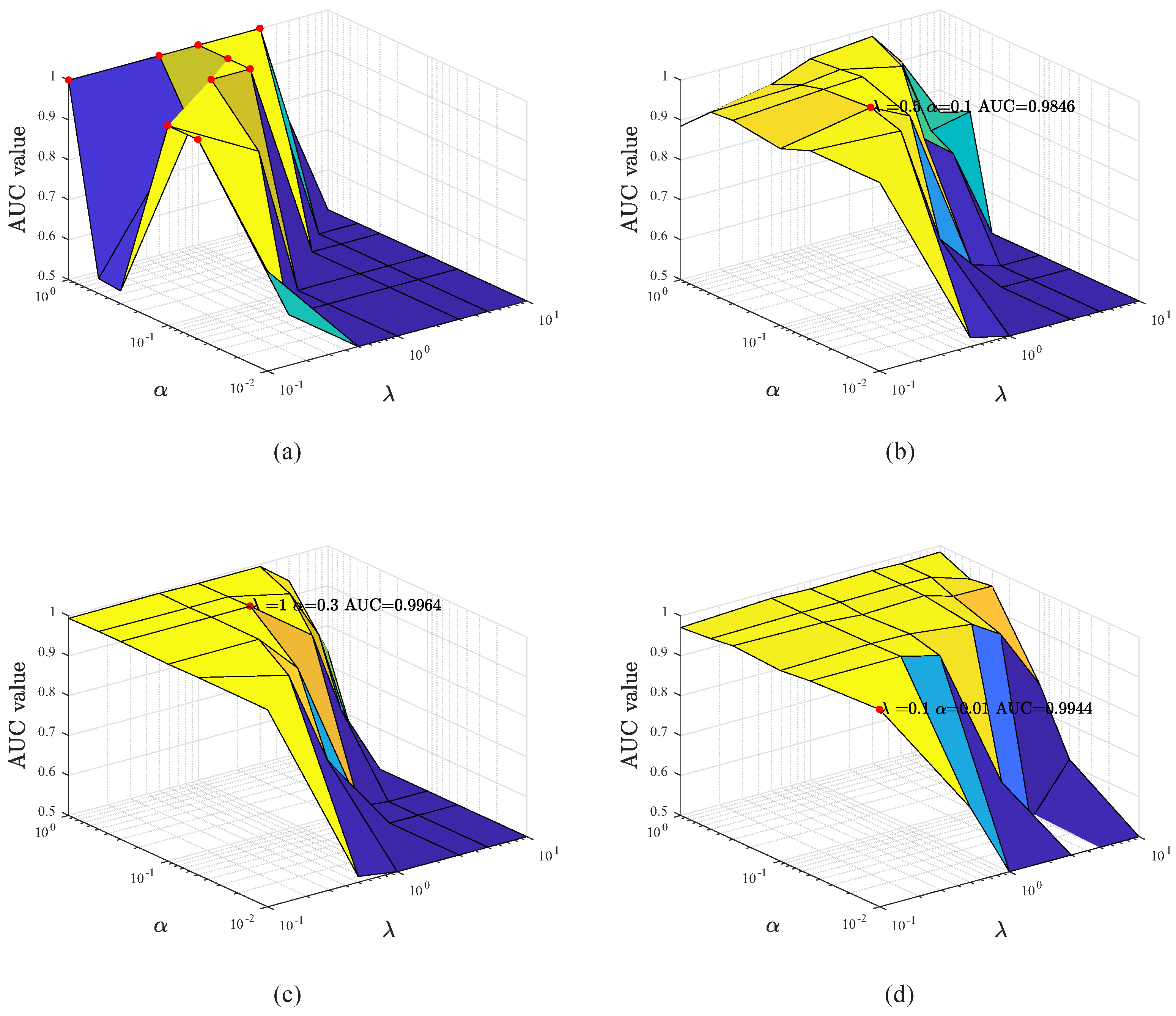
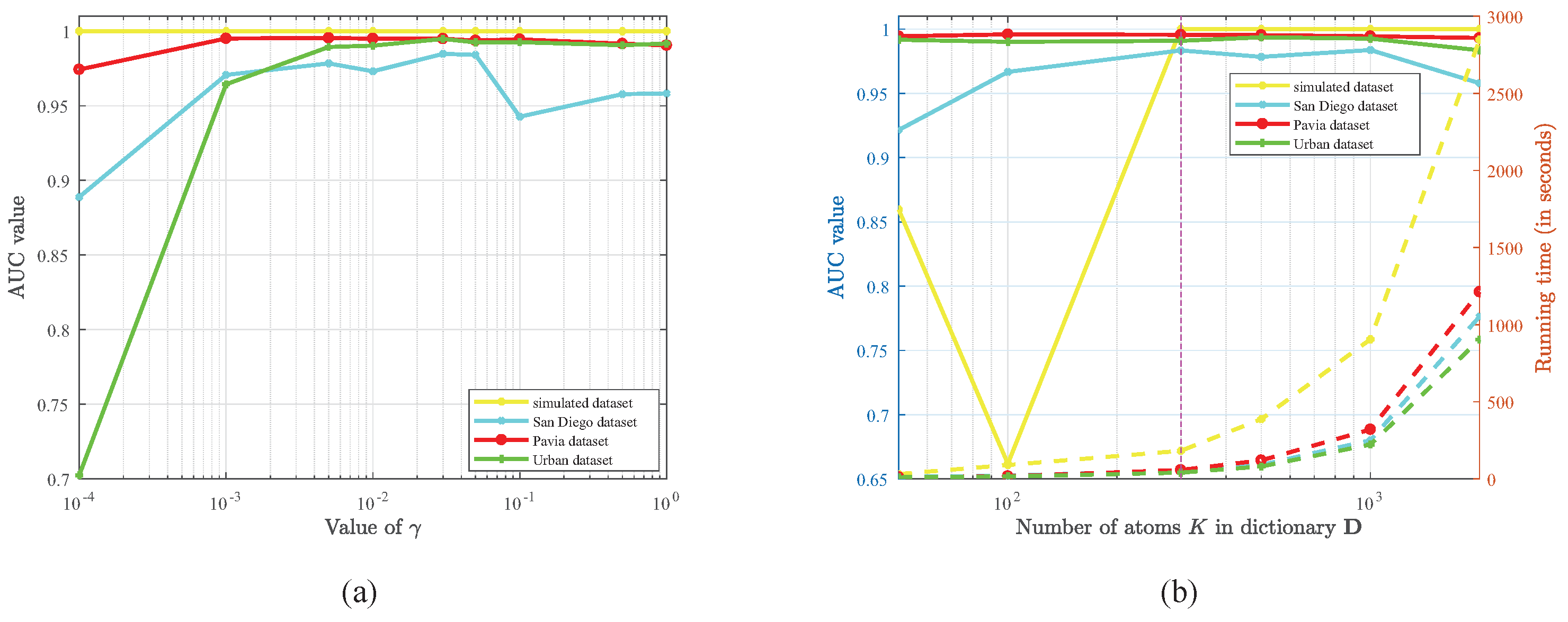
3.4. Parameters Analyses and Discussion

All the experiments were implemented with the MATLAB R2017a software on a computer with Inter Core I7-10700F CPU@ 2.90 GHz and 16 GB RAM. The key parameter K impacting the running time for our method is set to 300. The running times of different algorithms for four datasets are shown in

Table 2. The running time (in seconds) of different algorithms for four datasets including the simulated, San Diego airport, Pavia center, and Texas Coast urban.

Methods	Simulated	San Diego Airport	Pavia Center	Texas Coast Urban
GRX [12]	1.35	0.10	0.26	0.16
LRX [12]	45.90	50.14 (5,29)	23.59 (5,29)	60.25 (5,29)
BJSR [19]	26.63	6.15 (3,23)	6.39 (5,23)	5.93 (5,23)
CRD [21]	1631.15 (5,23)	297.06 (5,23)	498.54 (5,29)	286.66 (5,23)
LSMAD [25]	15.91	10.48	7.75	13.04
LRASR [27]	262.91	37.70	47.93	40.45
KIFD [41]	377.42	58.41	59.06	54.49
LCLRR	182.51	54.23	58.13	40.89

. It can be observed that the GRX method runs the fastest, and the CRD method takes the most time. The time complexity of our method is acceptable, considering its excellent detection capability.

There are four parameters involved in our method, namely the sparsity regularization parameter $\lambda$, the locality regularization parameter $\alpha$, the dictionary regularization parameter $\gamma$, and the number of atoms K in dictionary $\mathbf{D}$. We use the changing curve of AUC value to assess the influence of those parameters on the detection performance.

Firstly, the effects of the parameters $\lambda$ and $\alpha$ are discussed. Before experiment, the $\gamma$ and K are fixed to $0.05$ and 300, respectively. The value of $\lambda$ is set to $0.1,0.5,1,3,5,10$ in sequence, and the value of $\alpha$ is set to $0.01,0.05,0.1,0.3,0.5,1$ in sequence. We compute the AUC values of our algorithm using different parameter combination for four datasets, and then plot the surface diagram of AUC value changes in Figure 11. The best results are labeled with red spot, and corresponding AUC values and parameter combinations are marked nearby. It is worth noting that the AUC value equaling to 0.5 indicate the parameter combination is inappropriate. For the simulated dataset, $\lambda =1$ is preferable, and the ratio of $\lambda$ and $\alpha$ is less than 10. For other three real datesets, the rule of parameter selection is similar. $\lambda$ and $\alpha$ are preferably less than 1, and their ratio is less than 10. In all, the scope of working parameter is large, and they are easy to select. Furthermore, the locality regularization parameter $\alpha$ is discussed separately. We take the detection maps for the San Diego dataset as an example. we fix the $\lambda$ to $0.5$, and set $\alpha$ to $0.01,0.05,0.1,0.3,0.5,1$ in sequence. The final six detection maps are depicted in Figure 12. It can be observed that the anomaly objects become obvious as $\alpha$ increases. In other words, the $DP$ is positively associated with parameter $\alpha$. However, the background pixels also become evident, leading to high $FAR$. Considering the $DP$ and $FAR$ comprehensively, $\alpha =0.3$ is preferable. Based on these results, we can conclude that increasing the weight of the locality constrained term can make our method capture more local details.

Secondly, the influence of regularization parameter $\gamma$ is also discussed. The $\lambda$ and $\alpha$ are set according to the results in Figure 11. The parameter K is set to 300, and the value of $\gamma$ is set to $0.0001,0.001,0.005,0.01,0.03,0.05,0.1,0.5,1$ in sequence. The curves of AUC value changes for four datasets are shown in Figure 13a. The $\gamma$ have obvious effects for the San Diego airport and Texas Coast urban datasets, but little effect on the simulated and Pavia center datasets. The $\gamma =0.05$ is an optimal selection for four datasets.

Thirdly, the number of atoms in dictionary is an important parameter, which influence the results of weight matrix $\mathbf{W}$ and coefficient matrix $\mathbf{S}$. Similarly, the other parameters are fixed in advance. The K is set to $50,100,300,500,1000,2000$ in turn, and the changing curves of AUC value and running time are shown in Figure 13b. The parameter K has some impact for the San Diego airport dataset, but little impact for other three datasets. The main reason for this is that the background materials of the San Diego airport dataset is more complex than others. Obviously, the running time increases rapidly along with the K. The $K=300$ is good choice for four datasets, considering the detection performance and time complexities comprehensively.

4. Conclusions

In this paper, a novel hyperspectral anomaly detection method with the LCLRR model was proposed. Unlike most of the existing HAD algorithms based on LRR model, our proposed method introduced a locality constrained LRR model to model the background and anomaly part. By adding the locality constrained term, our model can force the pixelsr with small distances in HSI to have similar representation coefficients after the low rank decomposition process. Furthermore, the dictionary learning process and LRR is a whole process, the residual matrix referring to anomaly, coefficient matrix, and dictionary matrix can be obtained simultaneously. The experiments on simulated dataset and three real datasets demonstrated that our method can detect anomalies accurately. Significantly, our method can suppress both the background and noises effectively, yielding a clear and accurate detection map. Three metrics including ROC curve, AUC value, box plot, all demonstrate that our algorithm is better than other state-of-art algorithms. In the future, how to extend the LCLRR model into other remote sensing tasks is our next research interest.

References

1. Ghamisi, P.; Yokoya, N.; Li, J.; Liao, W.; Liu, S.; Plaza, J.; Rasti, B.; Plaza, A. Advances in Hyperspectral Image and Signal Processing: A Comprehensive Overview of the State of the Art. IEEE Geosci. Remote Sens. Mag. 2017, 5, 37–78. [Google Scholar] [CrossRef] [Green Version]
2. Li, X.; Yuan, Z.; Wang, Q. Unsupervised deep noise modeling for hyperspectral image change detection. Remote Sens. 2019, 11, 258. [Google Scholar] [CrossRef] [Green Version]
3. Chen, M.; Wang, Q.; Li, X. Discriminant analysis with graph learning for hyperspectral image classification. Remote Sens. 2018, 10, 836. [Google Scholar] [CrossRef] [Green Version]
4. Gao, Y.; Feng, Y.; Yu, X. Hyperspectral Target Detection with an Auxiliary Generative Adversarial Network. Remote Sens. 2021, 13, 4454. [Google Scholar] [CrossRef]
5. Su, H.; Wu, Z.; Zhang, H.; Du, Q. Hyperspectral Anomaly Detection: A Survey. IEEE Geosci. Remote Sens. Mag. 2021, 2–28. [Google Scholar] [CrossRef]
6. Gao, L.; Yang, B.; Du, Q.; Zhang, B. Adjusted spectral matched filter for target detection in hyperspectral imagery. Remote Sens. 2015, 7, 6611–6634. [Google Scholar] [CrossRef] [Green Version]
7. Matteoli, S.; Diani, M.; Corsini, G. A tutorial overview of anomaly detection in hyperspectral images. IEEE Aerosp. Electron. Syst. Mag. 2010, 25, 5–28. [Google Scholar] [CrossRef]
8. Eismann, M.T.; Stocker, A.D.; Nasrabadi, N.M. Automated hyperspectral cueing for civilian search and rescue. Proc. IEEE 2009, 97, 1031–1055. [Google Scholar] [CrossRef]
9. Theiler, J.; Ziemann, A.; Matteoli, S.; Diani, M. Spectral variability of remotely sensed target materials: Causes, models, and strategies for mitigation and robust exploitation. IEEE Geosci. Remote Sens. Mag. 2019, 7, 8–30. [Google Scholar] [CrossRef]
10. Kruse, F.A.; Boardman, J.W.; Huntington, J.F. Comparison of airborne hyperspectral data and EO-1 Hyperion for mineral mapping. IEEE Trans. Geosci. Remote Sens. 2003, 41, 1388–1400. [Google Scholar] [CrossRef] [Green Version]
11. Transon, J.; d’Andrimont, R.; Maugnard, A.; Defourny, P. Survey of hyperspectral earth observation applications from space in the sentinel-2 context. Remote Sens. 2018, 10, 157. [Google Scholar] [CrossRef] [Green Version]
12. Reed, I.S.; Yu, X. Adaptive multiple-band CFAR detection of an optical pattern with unknown spectral distribution. IEEE Trans. Acoust. Speech Signal Process. 1990, 38, 1760–1770. [Google Scholar] [CrossRef]
13. Guo, Q.; Zhang, B.; Ran, Q.; Gao, L.; Li, J.; Plaza, A. Weighted-RXD and Linear Filter-Based RXD: Improving Background Statistics Estimation for Anomaly Detection in Hyperspectral Imagery. IEEE J. Sel. Top. Appl. Earth Obs. Remote Sens. 2014, 7, 2351–2366. [Google Scholar] [CrossRef]
14. Taitano, Y.P.; Geier, B.A.; Bauer, K.W. A locally adaptable iterative RX detector. EURASIP J. Adv. Signal Process. 2010, 2010, 341908. [Google Scholar] [CrossRef] [Green Version]
15. Zhang, Y.; Fan, Y.; Xu, M. A Background-Purification-Based Framework for Anomaly Target Detection in Hyperspectral Imagery. IEEE Geosci. Remote Sens. Lett. 2020, 17, 1238–1242. [Google Scholar] [CrossRef]
16. Kwon, H.; Nasrabadi, N.M. Kernel RX-algorithm: A nonlinear anomaly detector for hyperspectral imagery. IEEE Trans. Geosci. Remote Sens. 2005, 43, 388–397. [Google Scholar] [CrossRef]
17. Zhou, J.; Kwan, C.; Ayhan, B.; Eismann, M.T. A Novel Cluster Kernel RX Algorithm for Anomaly and Change Detection Using Hyperspectral Images. IEEE Trans. Geosci. Remote Sens. 2016, 54, 6497–6504. [Google Scholar] [CrossRef]
18. Chen, Y.; Nasrabadi, N.M.; Tran, T.D. Sparse representation for target detection in hyperspectral imagery. IEEE J. Sel. Top. Signal Process. 2011, 5, 629–640. [Google Scholar] [CrossRef]
19. Li, J.; Zhang, H.; Zhang, L.; Ma, L. Hyperspectral anomaly detection by the use of background joint sparse representation. IEEE J. Sel. Top. Appl. Earth Obs. Remote Sens. 2015, 8, 2523–2533. [Google Scholar] [CrossRef]
20. Ma, D.; Yuan, Y.; Wang, Q. Hyperspectral anomaly detection via discriminative feature learning with multiple-dictionary sparse representation. Remote Sens. 2018, 10, 745. [Google Scholar] [CrossRef] [Green Version]
21. Li, W.; Du, Q. Collaborative representation for hyperspectral anomaly detection. IEEE Trans. Geosci. Remote Sens. 2014, 53, 1463–1474. [Google Scholar] [CrossRef]
22. Hou, Z.; Li, W.; Gao, L.; Zhang, B.; Ma, P.; Sun, J. A Background Refinement Collaborative Representation Method with Saliency Weight for Hyperspectral Anomaly Detection. In Proceedings of the 2020 IEEE International Geoscience and Remote Sensing Symposium, Waikoloa, HI, USA, 26 September–2 October 2020; pp. 2412–2415. [Google Scholar]
23. Sun, W.; Liu, C.; Li, J.; Lai, Y.M.; Li, W. Low-rank and sparse matrix decomposition-based anomaly detection for hyperspectral imagery. J. Appl. Remote Sens. 2014, 8, 083641. [Google Scholar] [CrossRef]
24. Zhou, T.; Tao, D. Godec: Randomized low-rank & sparse matrix decomposition in noisy case. In Proceedings of the 28th International Conference on Machine Learning, Bellevue, WA, USA, 28 June–2 July 2011; pp. 33–40. [Google Scholar]
25. Zhang, Y.; Du, B.; Zhang, L.; Wang, S. A Low-Rank and Sparse Matrix Decomposition-Based Mahalanobis Distance Method for Hyperspectral Anomaly Detection. IEEE Trans. Geosci. Remote Sens. 2016, 54, 1376–1389. [Google Scholar] [CrossRef]
26. Qu, Y.; Wang, W.; Guo, R.; Ayhan, B.; Kwan, C.; Vance, S.; Qi, H. Hyperspectral anomaly detection through spectral unmixing and dictionary-based low-rank decomposition. IEEE Trans. Geosci. Remote Sens. 2018, 56, 4391–4405. [Google Scholar] [CrossRef]
27. Xu, Y.; Wu, Z.; Li, J.; Plaza, A.; Wei, Z. Anomaly detection in hyperspectral images based on low-rank and sparse representation. IEEE Trans. Geosci. Remote Sens. 2015, 54, 1990–2000. [Google Scholar] [CrossRef]
28. Song, S.; Yang, Y.; Zhou, H.; Chan, J.C.W. Hyperspectral Anomaly Detection via Graph Dictionary-Based Low Rank Decomposition with Texture Feature Extraction. Remote Sens. 2020, 12, 3966. [Google Scholar] [CrossRef]
29. Liu, G.; Lin, Z.; Yan, S.; Sun, J.; Yu, Y.; Ma, Y. Robust recovery of subspace structures by low-rank representation. IEEE Trans. Pattern Anal. Mach. Intell. 2012, 35, 171–184. [Google Scholar] [CrossRef] [Green Version]
30. Wang, Q.; He, X.; Li, X. Locality and structure regularized low rank representation for hyperspectral image classification. IEEE Trans. Geosci. Remote Sens. 2018, 57, 911–923. [Google Scholar] [CrossRef] [Green Version]
31. Li, X.; Chen, M.; Nie, F.; Wang, Q. A multiview-based parameter free framework for group detection. In Proceedings of the Thirty-First AAAI Conference on Artificial Intelligence, San Francisco, CA, USA, 4–9 February 2017; pp. 4147–4153. [Google Scholar]
32. Lin, Z.; Chen, M.; Ma, Y. The augmented lagrange multiplier method for exact recovery of corrupted low-rank matrices. arXiv 2010, arXiv:1009.5055. [Google Scholar]
33. Bertsekas, D.P. Constrained Optimization and Lagrange Multiplier Methods; Academic Press: Cambridge, MA, USA, 2014. [Google Scholar]
34. Li, H.; Feng, R.; Wang, L.; Zhong, Y.; Zhang, L.; Wei, L. Low-Rank Representation Incorporating Local Spatial Constraint for Hyperspectral Anomaly Detection. In Proceedings of the 2021 IEEE International Geoscience and Remote Sensing Symposium, Brussels, Belgium, 11–16 July 2021; pp. 4424–4427. [Google Scholar]
35. Li, X.; Chen, M.; Nie, F.; Wang, Q. Locality adaptive discriminant analysis. In Proceedings of the IJCAI, Melbourne, Australia, 19–25 August 2017; pp. 2201–2207. [Google Scholar]
36. Cox, M.A.; Cox, T.F. Multidimensional scaling. In Handbook of Data Visualization; Springer: Berlin/Heidelberg, Germany, 2008; pp. 315–347. [Google Scholar]
37. Yin, H.F.; Wu, X.J.; Kittler, J. Face Recognition via Locality Constrained Low Rank Representation and Dictionary Learning. arXiv 2019, arXiv:1912.03145. [Google Scholar]
38. Pan, L.; Li, H.C.; Chen, X.D. Locality constrained low-rank representation for hyperspectral image classification. In Proceedings of the 2016 IEEE International Geoscience and Remote Sensing Symposium, Beijing, China, 10–15 July 2016; pp. 493–496. [Google Scholar]
39. Yang, Y.; Zhang, J.; Song, S.; Liu, D. Hyperspectral anomaly detection via dictionary construction-based low-rank representation and adaptive weighting. Remote Sens. 2019, 11, 192. [Google Scholar] [CrossRef] [Green Version]
40. Yuan, Y.; Ma, D.; Wang, Q. Hyperspectral Anomaly Detection by Graph Pixel Selection. IEEE Trans. Cybern. 2016, 46, 3123–3134. [Google Scholar] [CrossRef]
41. Li, S.; Zhang, K.; Duan, P.; Kang, X. Hyperspectral anomaly detection with kernel isolation forest. IEEE Trans. Geosci. Remote Sens. 2019, 58, 319–329. [Google Scholar] [CrossRef]
42. Liu, F.T.; Ting, K.M.; Zhou, Z.H. Isolation forest. In Proceedings of the 2008 Eighth IEEE International Conference on Data Mining, Pisa, Italy, 15–19 December 2008; pp. 413–422. [Google Scholar]
43. Kerekes, J. Receiver operating characteristic curve confidence intervals and regions. IEEE Geosci. Remote Sens. Lett. 2008, 5, 251–255. [Google Scholar] [CrossRef] [Green Version]
44. Williamson, D.F.; Parker, R.A.; Kendrick, J.S. The box plot: A simple visual method to interpret data. Ann. Intern. Med. 1989, 110, 916–921. [Google Scholar] [CrossRef]
Figure 1. The flowchart of the proposed LCLRR method.
Remotesensing 14 01327 g001
Figure 2. The pseudo-color images composed of 10th, 70th, and 100th spectral bands and their corresponding reference maps: (a) Simulated. (b) San Diego airport. (c) Pavia center. (d) Texas Coast urban.
Remotesensing 14 01327 g002
Figure 3. The detection maps of different algorithms for the simulated dataset, and the parameters in brackets are sizes of double-window used in corresponding algorithms. (a) Reference map. (b) GRX. (c) LRX (5, 29). (d) BJSR (3, 23). (e) CRD (3, 23). (f) LSMAD. (g) LRASR. (h) KIFD. (i) LCLRR.
Remotesensing 14 01327 g003
Figure 4. The ROC curves and box plots of different algorithms for the simulated dataset. (a) ROC curve. (b) box plot.
Remotesensing 14 01327 g004
Figure 5. The detection maps of different algorithms for the San Diego airport dataset, the parameters in brackets are sizes of double-window used in corresponding algorithms. (a) Reference map. (b) GRX. (c) LRX (5, 29). (d) BJSR (3, 23). (e) CRD (3, 23). (f) LSMAD. (g) LRASR. (h) KIFD. (i) LCLRR.
Remotesensing 14 01327 g005
Figure 6. The ROC curves and box plots of different algorithms for the San Diego airport dataset. (a) ROC curve. (b) box plot.
Remotesensing 14 01327 g006
Figure 7. The detection maps of different algorithms for the Pavia center dataset, the parameters in brackets are sizes of double-window used in corresponding algorithms. (a) Reference map. (b) GRX. (c) LRX (5,29). (d) BJSR (3,23). (e) CRD (3,23). (f) LSMAD. (g) LRASR. (h) KIFD. (i) LCLRR.
Remotesensing 14 01327 g007
Figure 8. The ROC curves and box plots of different algorithms for the Pavia center dataset. (a) ROC curve. (b) box plot.
Remotesensing 14 01327 g008
Figure 9. The detection maps of different algorithms for the Texas Coast urban dataset, the parameters in brackets are sizes of double-window used in corresponding algorithms. (a) Reference map. (b) GRX. (c) LRX (5, 29). (d) BJSR (3, 23). (e) CRD (3, 23). (f) LSMAD. (g) LRASR. (h) KIFD. (i) LCLRR.
Remotesensing 14 01327 g009
Figure 10. The ROC curves and box plots of different algorithms for the Texas Coast urban dataset. (a) ROC curve. (b) box plot.
Remotesensing 14 01327 g010
Figure 11. The influence of parameter λ and α on the detection performance for four datasets. (a) Simulated. (b) San Diego airport. (c) Pavia center. (d) Texas Coast urban.
Remotesensing 14 01327 g011
Figure 12. The detection maps with different settings of α for the San Diego airport dataset. (a) α = 0.01 . (b) α = 0.05 . (c) α = 0.1 . (d) α = 0.3 . (e) α = 0.5 . (f) α = 1 .
Remotesensing 14 01327 g012
Figure 13. (a) The influence of parameter γ on the detection performance for four datasets. (b) The influence of parameter K on the detection performance and running time for four datasets.
Remotesensing 14 01327 g013