Abstract
As a sensitive indicator for climate change, the spring phenology of alpine grassland on the Qinghai–Tibet Plateau (QTP) has received extensive concern over past decade. It has been demonstrated that temperature and precipitation/snowfall play an important role in driving the green-up in alpine grassland. However, the spatial differences in the temperature and snowfall driven mechanism of alpine grassland green-up onset are still not clear. This manuscript establishes a set of process-based models to investigate the climate variables driving spring phenology and their spatial differences. Specifically, using 500 m three-day composite MODIS NDVI datasets from 2000 to 2015, we first estimated the land surface green-up onset (LSGO) of alpine grassland in the QTP. Further, combining with daily air temperature and precipitation datasets from 2000 to 2015, we built up process-based models for LSGO in 86 meteorological stations in the QTP. The optimum models of the stations separating climate drivers spatially suggest that LSGO in grassland is: (1) controlled by temperature in the north, west and south of the QTP, where the precipitation during late winter and spring is less than 20 mm; (2) driven by the combination of temperature and precipitation in the middle, east and southwest regions with higher precipitation and (3) more likely controlled by both temperature and precipitation in snowfall dominant regions, since the snow-melting process has negative effects on the air temperature. The result dictates that snowfall and rainfall should be concerned separately in the improvement of the spring phenology model of the alpine grassland ecosystem.
1. Introduction
The Earth has experienced significant warming since the industrial revolution (IPCC, 2013), and the warming rate in the Qinghai–Tibet Plateau (QTP) over the past five decades is twice the global average [1]. Rapid warming has significantly affected the biogeochemical cycles [1] and the ecological environment [2] in QTP grassland, which covers 66% of the area. In particular, the warming-deduced variation in vegetation spring phenology directly affects the grassland’s net primary productivity and herbage production, which has a strong impact on the development of the regional economy. As a result, the date of green-up onset, which represents the start of the growing season in grasslands on the QTP, has recently been extensively investigated [3,4,5,6,7,8,9,10,11,12,13,14,15,16,17,18]. The majority of previous research is based on statistical methods to reveal the relationship between the spring phenology and climate variables [3,6,7,10,12,15,16,19,20], however, process models and process simulations of green-up onset are not well applied, and the climate control mechanism of grassland green-up onset and the spatial difference are not well investigated [11,21]. It has been recognized that a process-based model could effectively and accurately simulate the plant development process and the phenological phase based on various climate variables, such as temperature, precipitation and photoperiod [22]. Therefore, it is important to develop and apply the process-based spring phenology model for scientifically understanding the influence mechanism of climate change on the green-up date of grasslands and analyzing the spatial difference on the QTP for dealing with climate change, ecological protection and animal husbandry development.
Vegetation spring phenology has been commonly modeled by associating ground based phenology observations for individual species with meteorological data [22].This is also true on the QTP [11]. Although temperature is regarded as the main driving factor for the simulation of woody plant spring phenology [23,24], temperature, precipitation and their coupling effect are usually integrated together in the construction of a spring phenology model in grasslands [11,21,25,26]. Specifically, grassland green-up has been linked to air temperature, precipitation and their coupling effect as observed in meteorological stations [3,4,5,10,27], suggesting that precipitation or snowfall have much stronger controls on grassland green-up [7,11,28]. Moreover, a process-based phenology model, which was established based on multi-stations, multi-species and long term series of herb green-up dates from ground observations in the east and south of the QTP, indicates that late winter and spring snowfall is an important factor that affects the herb green-up [11]. However, the ground phenology observations are very limited and are mainly distributed in the margin of the QTP [11,29,30], so that the resultant phenological models only represent the corresponding phenological sites, but they are generally unable to explain detailed spatial patterns of climate controls on alpine grassland spring phenology on a large scale.
Specifically, varieties of models have been proposed to simulate the vegetation spring phenology [31], such as the GDD (growing degree days) model [32,33,34], sequential model, parallel model, alternating model and the unified model [23], with temperature as the only driving factor. However, these models are mainly developed for the simulation of spring phenology (leaf unfolding/leaf-out/budburst) for woody plants. For herbaceous plants with different physiological characteristics, because of the existing precipitation’s control over the spring phenology, precipitation was embedded in the above-mentioned models to improve the simulation of the green-up date [11,25]. However, either for woody plants or herbaceous plants, the models were designed based on the physiological processes of individual plants to simulate plant phenology at the species-level, which is dependent on limited plant individual phenology observation and could not be generalized to the land surface in a large area.
In contrast, land surface phenology derived from satellite data provides exhaustive spatial distributions, which can be used to establish much more robust phenology models to illustrate climate impacts on phenology variation on the QTP [21,35]. However, current detections of land surface phenology vary greatly, with different methods of processing the noisy time series of satellite observations [36,37]. Most of the phenology detections contain large uncertainties compared with ground observations [37]. Thus, it is necessary to evaluate the process-based simulation for the land surface green-up onset (LSGO) based on in situ observations.
In this study, we aim to investigate the following scientific questions: (1) can LSGO in grassland be used for the establishment of process-based models for exploring the spatial variation in climate drivers across QTP? (2) Can process-based models reveal the spatial difference of precipitation/snowfall control on alpine grassland spring phenology?
2. Materials and Methods
2.1. Study Area and Biomes
As the highest plateau in the world, the QTP is called ‘the roof of the world’, with a mean elevation exceeding 4000 m. Due to its special alpine environment, the QTP is the largest glacier store region, following the Arctic and Antarctica, and is called ‘the third pole’ of the Earth. The QTP is mainly distributed in China, including Tibet Autonomous Region, western Sichuan Province, part of Yunnan Province, Qinghai Province, southern Xinjiang Uygur Autonomous Region and part of Gansu province. The QTP climate is affected by south Asia monsoon in summer and prevailing westerlies in winter. From northwest to southeast, perennial mean air temperature ranges from −5 to 15.5 °C and multi-year average precipitation has been 16–1764 mm during the past three decades. Unique vegetation types have evolved on the QTP due to its special physic-geographical environment (Figure 1), which mainly consists of herbaceous plants that are steppe, meadow and alpine vegetation over 66% of the area [38]. Specifically, steppe is mainly dominated by Carex grass high-cold steppe, and the other types (which are only distributed in temperate regions on the northern QTP), include temperate tufted grass steppe, temperate tufted low grass nano-semi-shrub desert steppe and temperate grass forb meadow steppe [38]. Meadow is mainly dominated by Kobresia forb high-cold meadow, the other types including Carex grass and forb swamp meadow, grass and forb halophytic meadow and grass and forb meadow [38]. Alpine vegetation mainly consists of the composite family including alpine tundra and sparse vegetation and alpine cushion vegetation [38]. The other vegetation types include broad-leaved and coniferous forests in the south and southeast and shrub and cultivated vegetation in the east and margin of the east, but the areas are smaller [38].
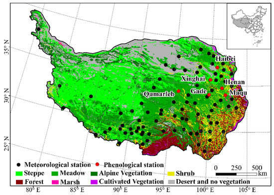
Figure 1.
Spatial distribution of vegetation type and meteorological and phenological stations on the QTP.
2.2. Ground Observations of Grass Green-Up and Meteorological Datasets
The grass green-up dates observed in fields are obtained from the China Meteorological Administration, which consists of 19 herb species over 6 phenological ground stations from 2000 to 2012. There are two to eight herb species being observed in each station (Table 1). The green-up date is observed by professional staff based on the same plant observation method with a united observation specification [39]. Specifically, the typical grassland in each station is selected, and then a 0.5 m × 0.5 m grassland quadrat is randomly extracted. The growing stages of 10 individuals for each species within the quadrat are observed every 2 days. The green-up date of the herbs is defined as the date when the young leaves in 50% of individuals grow higher than 1 cm over the ground. Usually, the observations are focused on the dominant species, such as poaceae, leguminosae and cyperaceae, and accompanying species, such as compositae, chenopodiaceae, liliaceous, rosaceae, umbrella and labiatae (Table 1). The mean green-up dates from multiple species in each station are used to establish the process-based models to evaluate the accuracy of land surface green-up onset (LSGO) (cf. Section 2.4).

Table 1.
The general information and observed herb species in phenological stations.
The meteorological datasets are derived from China’s meteorological data sharing service system in the China Meteorological Administration (http://cdc.nmic.cn/home.do (accessed on 22 December 2021)). The data include daily mean air temperature and daily precipitation from 2000 to 2015 in 86 stations (Figure 1). The stations are located at the elevation range from 1813.9 to 4900 m. Since the snowfall and rainfall data in late winter and spring (from 1 January to the multi-year mean green-up date) cannot be directly acquired for the meteorological stations, the snowfall data are defined as the accumulation of precipitation with daily mean air temperature below 0 °C [40]. The total rainfall is the accumulation of precipitation with daily mean air temperature above or equal to 0 °C.
2.3. Land Surface Green-Up Onset Dataset and Evaluation
Land surface spring phenology from 2000 to 2015 was estimated based on the Moderate Resolution Imaging SpectroRadiometer (MODIS) Nadir Bidirectional Reflectance Distribution Function (BRDF)-Adjusted Reflectance (NBAR) dataset (MCD43A4 Version 6) and Albedo Quality Product (MCD43A2) with a spatial resolution of 500 m and a temporal resolution of one day. Both MCD43A4 and MCD43A2 products were downloaded from the website (http://modis.gsfc.nasa.gov/ (accessed on 22 December 2021)) of the National Aeronautics and Space Administration (NASA). Daily normalized differential vegetation index (NDVI) was calculated from MCD43A4.
Three-day composite NDVI was computed first using maximum principle. Then, NDVI time series were fitted using the vegetation growing curve described in a logistic model, and curvature change rate was calculated to identify the phenological transition dates [41,42]. Specifically, a Hybrid Piecewise Logistic Model (HPLM) algorithm was first used to describe the temporal NDVI trajectory, optimizing the parameters of the logistic equation. Then, the curvature of the equation was computed. Finally, curvature variation (first derivative of curvature) was computed and the independent variable (day of year) which corresponds to the first extreme value of the dependent variable (first derivative of curvature) was defined as the land surface green-up onset (LSGO) (Figure 2). Details of the method are given in Zhang’s paper [43,44]. It should be note that the first growing cycle of grassland is only addressed in this study if there are two or more growing cycles. The land surface green-up onset dataset was evaluated using the multi-species mean green-up date in the six stations by mean absolute error (MAE) (Equation (1)), root mean square error (RMSE) (Equation (2)) and Pearson correlation coefficient (r) (Equation (3)), which are described as the followings.
where i is the sequence number of the year, n is the total number of years, is the mean green-up date of ground observations from multi species in the i-th year, is LSGO in the corresponding pixel, is the mean of multi-year ground observations in multi-species and is the mean of multi-year LSGO in one or multi-pixels.
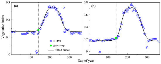
Figure 2.
MODIS NDVI curve fitting and green-up onset estimation. (a) is a sample pixel in steppe area and (b) is a sample pixel in meadow area in the QTP. The light green dot denotes the green-up onset point of alpine grassland on the fitting curves and the corresponding horizontal axis coordinate is the green-up onset.
In the evaluation, considering the uncertainties of remote sensing surface reflectance caused by the outliers and the spatial heterogeneity for the land surface phenology, field observations in each station are compared with LSGO within a set of pixel-window sizes to identify the optimum window size according to MAE, RMSE and r. The pixel-window size varies from one to twenty-one 500 m-pixels with the field station located in the center [45]. We then calculated the medium green-up onset of pixels within 9.5 km2 centered with the meteorological station in each window size to present the green-up onset of the alpine grassland of the meteorological station, which could also ensure the meteorological data are representative within this extent (usually less than 10 km2 [45]).
2.4. Establishment of Process-Based Model for Green-Up Dates
Process-based models for vegetation green-up date are established using daily mean air temperature and precipitation. The models are mainly divided into three groups [11,25], which are the traditional thermal time model, air temperature–precipitation parallel model and air temperature–precipitation sequential model. The traditional thermal time model assumes that vegetation begins to green-up when the accumulated temperature reaches to a critical value , which is described as (Equation (4)):
where is the initial day, which is usually defined as 1 January, y is the date of green-up onset and is the state of forcing temperature.is defined as Equations (5) and (6). is the degree-day base temperature indicating the linear response of green-up to the accumulation of temperature, a and b are the parameters and is the daily mean air temperature. Equation (5) is commonly used in previous studies [11,25]. However, the response of plant to temperature is usually nonlinear [46]. Thus, in our research, Equation (6) with logistic response function was used in the construction of the spring phenology model.
The air temperature–precipitation parallel model assumes that vegetation begins to green-up when the accumulated temperature reaches to a critical value (Equation (4)) and the state of forcing in precipitation () reaches a critical value from a date of t0 (Equations (7) and (8)):
where is the state of forcing in precipitation, is the daily precipitation (mm) and is the state of precipitation as a daily sum of the rate of precipitation.
The air temperature–precipitation sequential model assumes that the effect of air temperature on green-up (Equation (4)) is enforced after the state of forcing in precipitation reaches a critical value at the date of (Equation (9)), which means that, after this date, the forcing effect of air temperature on herb green-up will work until the date of green-up onset (y):
Four parameters of , , and should be determined for the air temperature-precipitation parallel and sequential models. The parameters of the three models are fitted using the simulated annealing algorithm of Metropolis [47] and are constrained by the lowest RMSE (root mean square error (Equation (10)) between simulated and observed green-up dates:
where is the observed green-up date in year i, is the simulated green-up date in year i and n is the number of the year. RMSE is a common indicator for the model evaluation. Usually, lower RMSE means better simulation accuracy.
The aforementioned three process-based models are established for ground observed grass green-up dates in each of six agrometeorological stations and for LSGO in each of eight-six meteorological stations. An optimum model for each station is chosen from the three process-based models to identify the factors driving green-up dates. The optimum model is selected based on the lowest value of Akaike information criterion (AIC) [11,25] (Equation (11)), which rates models in terms of parsimony and efficiency:
where is the observed green-up date in year i, is the simulated green-up date in year i, n is the number of the year and k is the number of the parameters. It is a commonly used index for the evaluation of the process-based phenology models [31,48], which could effectively avoid overfitting. It should be noted that the 16-year time series of LSGO in our research is enough for the phenology process-based simulation (usually more than 10 years) [11,25], so the data after 2015 are not included in our research.
3. Results
3.1. Land Surface Green-Up Onset of Alpine Grassland and Evaluation
The multi-year mean LSGO in grasslands varies from March to July (Figure 3). It shows that the green-up onset of alpine grassland tends to be later from the east to the west of the QTP. This spatial pattern is same as the results in previous studies [6,49], which demonstrates the high reliability of the MODIS green-up onset dataset. The MAE and RMSE of the 6 stations in different pixel windows are less than 20 days and the r of 4 stations shows significant positive correlations (Figure A1), which further demonstrated high reliability of the dataset.
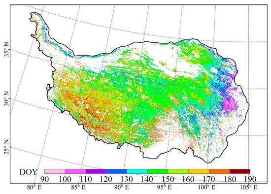
Figure 3.
Multi-year mean value of MODIS land surface green-up onset for pixels with detections for at least 10 years from 2000 to 2015.
3.2. Comparison of Process-Based Models between Ground Observations and LSGO
Table 2 presents the optimum models that are selected for the ground green-up date and the corresponding LSGO. In six agrometeorological stations (both phenological and meteorological data are available), the optimum model in each station is the best one to simulate green-up dates among the traditional thermal time model, air temperature–precipitation parallel model and air temperature–precipitation sequential model. The results indicate that the same type of optimum model is selected for both ground and LSGO green-up dates in two agrometeorological stations (Henan and Gade). However, all the optimal models for both ground observations and LSGO detections show that the green-up date is driven by the combination of air temperature and precipitation together (either air temperature–precipitation parallel or sequential model), except for the field green-up date in Xinghai, where the traditional thermal time model works better. Moreover, the RMSEs are very close to each other for ground observations and the LSGO based optimum model. The results overall suggest that the LSGO model is capable of simulating the grass green-up date with a similar accuracy as the ground based model.
Table 2.
Parameters of the optimum process-based models for ground observations and LSGO detections, respectively. Goodness of fit (R2), RMSE and AIC represent the quality of the optimum models at each station.
3.3. Process-Based Models of LSGO for All the Meteorological Stations
Figure 4a presents the optimal process-based models in each of 86 meteorological stations established based on medium LSGO in a window size of 9.5 km and daily mean air temperature and precipitation. The optimum models present clear spatial clusters geographically (Figure 4a). The thermal time model appears in 23 stations (27%) and is mainly distributed in the north, west and south of the QTP. This indicates that temperature drives green-up of grassland for the stations. In contrast, the temperature–precipitation parallel model (41% of stations) and temperature–precipitation sequential model (32% of stations) are spatially mixed and mainly distributed in the middle, east and southwest regions. This suggests that the green-up onset of grassland is mainly driven by the combination of air temperature and precipitation.
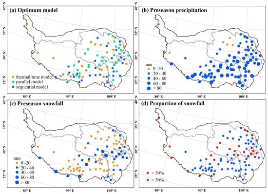
Figure 4.
The optimum process-based models for land surface green-up dates and their annual mean preseason precipitation/snowfall in 86 meteorological stations. (a) Optimum model, (b) annual mean preseason precipitation from January to April, (c) annual mean preseason snowfall January to April, and (d) proportion of snowfall.
3.4. The Spatial Pattern of Precipitation/Snowfall in the Stations
The annual mean preseason precipitation in each station spreads from 4.8 to 365 mm. On the whole, the precipitation in the south and southeast stations is higher than other stations, while the spatial difference is not obvious (Figure 4b). However, the annual mean preseason snowfall of the 86 stations shows obvious spatial difference (Figure 4c). Specifically, the stations with snowfall less than 20 mm are mainly distributed in the north, west and south QTP, while the stations with snowfall higher than 20 mm are mainly distributed in middle, east and southwest edge QTP. Furthermore, the stations with a proportion of snowfall (ration of snowfall and precipitation) higher than 50% were mainly distributed in the middle, east and southwest edge of the QTP (Figure 4b).
4. Discussion
4.1. Reliability of MODIS Land Surface Green-Up Onset for Construction Process-Based Model on the QTP
The process-based model for LSGO is expected to provide monitoring and prediction of phenology in vegetation communities across large scales. This could overcome the drawbacks in commonly used process-based phenology models established using extremely limited in situ observations. The process-based model using LSGO has shown advantages over a large region [35,50], such as the model for the woody leaf unfolding date in the deciduous broadleaf forest region of China [50].
However, although the MODIS LSGO has been used for the process simulation of alpine grassland green-up on the QTP [21], it is still full of uncertainty [36,37] and shows low predicted ability [21], which needs further evaluation based on in situ observations. Based on ground herb green-up date observation in six alpine grassland stations at the middle and east QTP, we evaluated the MODIS LSGO. Since the ground herb observation (tens of meters) does not spatially match with the MODIS pixel scale (hundreds of meters, community scale), it is hard to directly compare their difference [51]. However, we found that the MODIS LSGO could capture the green-up date variation in most of the stations. The simulation results from using both ground herb green-up date and LSGO at the same stations, such as lower RMSE and higher R2, supported our hypothesis that LSGO could perform well for the construction of process-based spring phenology. Specifically, the LSGO model simulation is similar to the multi-species mean green-up date observed from 33% of ground stations. However, the driving factors derived from the LSGO optimum model simulation are consistent with those from simulation of optimum models of the ground observations in 83% of stations. This suggests that the process-based optimum LSGO model could reflect well for the green-up onset climate driving factors in grassland, which is potentially capable of revealing the alpine grassland spring phenology climatic driving mechanism across the QTP.
4.2. Spatial Difference of the Optimum Process-Based Model for LSGO
The optimum LSGO model distinguishes the different climate drivers of grass green-up dates across 86 meteorological stations. The thermal time models and temperature–precipitation models reveal that both precipitation and temperature together trigger the grass green-up date in the middle, east and southwest regions, but thermal time alone drives the grass green-up timing in north, west and south areas (Figure 4a). This spatial difference in phenological forces is likely also associated with the amount of snowfall. A previous study based on the process-based model of the in situ herb green-up date shows that the green-up is mainly driven by air temperature in the stations with less than 20 mm snowfall, while it is mainly controlled by the coupling process between air temperature and precipitation in other regions [11]. Similarly, the optimum LSGO model in this study reveals that LSGO is manly driven by air temperature in the areas where precipitation in late winter and spring is less than 20 mm, while the LSGO is manly driven by air temperature and precipitation in other areas where precipitation is relatively high (Figure 4a,b). Since the regions with precipitation of less than 20 mm are mostly covered by less than 20 mm snowfall (Figure 4c,d), this suggests that air temperature is the main driver in triggering grass green-up in the regions with both precipitation and snowfall of less 20 mm. Nevertheless, the snow melting in the region with high snowfall is likely to reduce the air temperature, which could complicate climate controls on grass green-up. In this case, air temperature–precipitation models should be more appropriate for simulating grass green-up timing.
4.3. The Role of Snowfall in Driving Alpine Grassland Spring Phenology
Although temperature was regarded as the primary climatic factor controlling the plant spring phenology [52], the in situ species-level observations [28] and manipulative experiment [16] in alpine meadow on the QTP have demonstrated that soil moisture is also important in controlling green-up onset of alpine grassland on the QTP [28,53]. With the decrease in the soil moisture in spring, the green-up of the vegetation community was significantly delayed as the drought was induced [54]. Snowmelt is the only source of soil water in winter [28] in many areas of the QTP. By affecting soil moisture, snowfall could further control the alpine herb green-up. Moreover, based on multi-source remote sensing data streams, it has been reported that the snow cover melt date is positively correlated to the green-up onset in most areas of the QTP [17,27,55]. However, our research confirmed the snow control on alpine grassland on the QTP, but in limited spatial coverage. Except for the effect on soil moisture, the snow also has an indirect impact on the green-up onset of alpine grassland by reducing temperature when it melts [11]. The indirect control of snow on the green-up onset varies with the amount of snowfall in the late winter and early spring. The process-based model simulations in our research demonstrated that the green-up onset at the stations (80.7%) with larger amounts of snowfall (usually more than 20 mm) is mainly controlled by temperature and snowfall (31 stations in total, 25 stations’ optimum models are the parallel or sequential model, Figure 4a,c), which support the conjunction effect of snowfall and temperature. However, the dry winter with less snowfall in the alpine steppe distribution areas on the western and northern QTP resulted in temperature controlled green-up. Moreover, the proportion of snowfall in preseason precipitation is also an important factor that should be investigated. A higher proportion of snowfall means stronger impact on the temperature when the snowfall melts, which indicated a stronger control on the alpine grassland green-up onset. In fact, the conjunction effect of snowfall and temperature made the climate control on the alpine grassland more complex, which highlights that there should be different control degrees between preseason snowfall and rainfall on alpine grassland green-up onset, suggesting the snowfall and rainfall should be considered differently in the phenological module in the ecosystem model.
5. Conclusions
The optimum process-based models of the land surface green-up date are functionally consistent with the models of ground observed grass green-up date in 83% of the stations. This suggests that MODIS land surface green-up date is applicable for the construction of spring phenology process-based models and captures well the inter-annual variation in the ground green-up date in alpine grassland in the QTP. Thus, the process-based model of the land surface green-up date could be applied for monitoring grass growth across the QTP.
The spatial variation in optimum process-based models of land surface green-up date clearly distinguishes the different climate drivers controlling the grass green-up date across the QTP. The thermal time model is dominated in the north, west and south of the QTP, which implies that the green-up timing in grassland is mainly triggered by the spring temperature. In contrast, temperature–precipitation parallel and sequential models are mainly distributed in the middle, east and southwest, where the grassland green-up date is driven by the combination of temperature and precipitation.
Finally, the grassland green-up on the QTP could also be influenced by snowfall. The impact from the snowfall and rainfall to the grassland green-up is different because the snow melting process has negative effects on the air temperature. Future research is needed to separate snowfall and rainfall during late winter and spring in process-based phenological models.
Author Contributions
All authors made great contributions to the work. Specific contributions include research design (S.A.), data collection and image processing (S.A., X.Z.), data analysis (S.A.) and manuscript preparation (S.A., X.Z., S.R.). All authors have read and agreed to the published version of the manuscript.
Funding
This work was funded by the National Natural Science Foundation of China under grant nos. 42001101 and R&D Program of Beijing Municipal Education Commission (KM202111417013).
Data Availability Statement
Not applicable.
Acknowledgments
The authors thank the Meteorological Information Center of the China Meteorological Administration for providing phenological and meteorological datasets. We also thank NASA for providing free and ready access to the MODIS data.
Conflicts of Interest
The authors declare no conflict of interest.
Appendix A
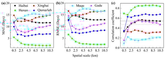
Figure A1.
The evaluation of MODIS land surface green-up onset. MAE (a), RMSE (b) and correlation coefficient (c) between multi-species mean green-up date and NDVI retrieved median green-up onset within different window sizes from 2000 to 2012. X-axis is the window size from 0.5 to 10.5 km. Y-axis is the MAE (days), RMSE (days) and correlation coefficient, respectively. Values above the high and low dashed lines in (c) denote significantly positive correlation at p < 0.05 and p < 0.1 levels, respectively. The symbols with different shapes and colors represent different phenological stations.
References
- Chen, H.; Zhu, Q.; Peng, C.; Wu, N.; Wang, Y.; Fang, X.; Gao, Y.; Zhu, D.; Yang, G.; Tian, J.; et al. The impacts of climate change and human activities on biogeochemical cycles on the Qinghai-Tibetan Plateau. Glob. Chang. Biol. 2013, 19, 2940–2955. [Google Scholar] [CrossRef] [PubMed]
- Yang, K.; Wu, H.; Qin, J.; Lin, C.; Tang, W.; Chen, Y. Recent climate changes over the Tibetan Plateau and their impacts on energy and water cycle: A review. Glob. Planet. Chang. 2014, 112, 79–91. [Google Scholar] [CrossRef]
- Yu, H.; Luedeling, E.; Xu, J. Winter and spring warming result in delayed spring phenology on the Tibetan Plateau. Proc. Natl. Acad. Sci. USA 2010, 107, 22151–22156. [Google Scholar] [CrossRef] [Green Version]
- Piao, S.; Cui, M.; Chen, A.; Wang, X.; Ciais, P.; Liu, J.; Tang, Y. Altitude and temperature dependence of change in the spring vegetation green-up date from 1982 to 2006 in the Qinghai-Xizang Plateau. Agric. For. Meteorol. 2011, 151, 1599–1608. [Google Scholar] [CrossRef]
- Shen, M.; Tang, Y.; Chen, J.; Zhu, X.; Zheng, Y. Influences of temperature and precipitation before the growing season on spring phenology in grasslands of the central and eastern Qinghai-Tibetan Plateau. Agric. For. Meteorol. 2011, 151, 1711–1722. [Google Scholar] [CrossRef]
- Shen, M.; Zhang, G.; Cong, N.; Wang, S.; Kong, W.; Piao, S. Increasing altitudinal gradient of spring vegetation phenology during the last decade on the Qinghai–Tibetan Plateau. Agric. For. Meteorol. 2014, 189–190, 71–80. [Google Scholar] [CrossRef]
- Shen, M.; Piao, S.; Cong, N.; Zhang, G.; Jassens, I.A. Precipitation impacts on vegetation spring phenology on the Tibetan Plateau. Glob. Chang. Biol. 2015, 21, 3647–3656. [Google Scholar] [CrossRef] [Green Version]
- Shen, M.; Piao, S.; Chen, X.; An, S.; Fu, Y.H.; Wang, S.; Cong, N.; Janssens, I.A. Strong impacts of daily minimum temperature on the green-up date and summer greenness of the Tibetan Plateau. Glob. Chang. Biol. 2016, 22, 3057–3066. [Google Scholar] [CrossRef]
- Shrestha, U.B.; Gautam, S.; Bawa, K.S. Widespread climate change in the Himalayas and associated changes in local ecosystems. PLoS ONE 2012, 7, e36741. [Google Scholar] [CrossRef] [Green Version]
- Zhang, G.; Zhang, Y.; Dong, J.; Xiao, X. Green-up dates in the Tibetan Plateau have continuously advanced from 1982 to 2011. Proc. Natl. Acad. Sci. USA 2013, 110, 4309–4314. [Google Scholar] [CrossRef] [Green Version]
- Chen, X.; An, S.; Inouye, D.W.; Schwartz, M.D. Temperature and snowfall trigger alpine vegetation green-up on the world’s roof. Glob. Chang. Biol. 2015, 21, 3635–3646. [Google Scholar] [CrossRef] [PubMed]
- Zheng, Z.; Zhu, W.; Chen, G.; Jiang, N.; Fan, D.; Zhang, D. Continuous but diverse advancement of spring-summer phenology in response to climate warming across the Qinghai-Tibetan Plateau. Agric. For. Meteorol. 2016, 223, 194–202. [Google Scholar] [CrossRef]
- Yang, B.; He, M.; Shishov, V.; Tychkov, I.; Vaganov, E.; Rossi, S.; Ljungqvist, F.C.; Bräuning, A.; Grießinger, J. New perspective on spring vegetation phenology and global climate change based on Tibetan Plateau tree-ring data. Proc. Natl. Acad. Sci. USA 2017, 114, 6966–6971. [Google Scholar] [CrossRef] [PubMed] [Green Version]
- Wang, Y.; Case, B.; Rossi, S.; Dawadi, B.; Liang, E.; Ellison, A.M. Frost controls spring phenology of juvenile Smith fir along elevational gradients on the southeastern Tibetan Plateau. Int. J. Biometeorol. 2019, 63, 963–972. [Google Scholar] [CrossRef]
- Li, X.; Guo, W.; Chen, J.; Ni, X.; Wei, X. Responses of vegetation green-up date to temperature variation in alpine grassland on the Tibetan Plateau. Ecol. Indic. 2019, 104, 390–397. [Google Scholar] [CrossRef]
- Ganjurjav, H.; Gornish, E.S.; Hu, G.; Schwartz, M.W.; Wan, Y.; Li, Y.; Gao, Q. Warming and precipitation addition interact to affect plant spring phenology in alpine meadows on the central Qinghai-Tibetan Plateau. Agric. For. Meteorol. 2020, 287, 107943. [Google Scholar] [CrossRef]
- Huang, K.; Zhang, Y.; Tagesson, T.; Brandt, M.; Wang, L.; Chen, N.; Zu, J.; Jin, H.; Cai, Z.; Tong, X.; et al. The confounding effect of snow cover on assessing spring phenology from space: A new look at trends on the Tibetan Plateau. Sci. Total Environ. 2021, 756, 144011. [Google Scholar] [CrossRef]
- Sun, Q.; Li, B.; Jiang, Y.; Chen, X.; Zhou, G. Declined trend in herbaceous plant green-up dates on the Qinghai-Tibetan Plateau caused by spring warming slowdown. Sci. Total Environ. 2021, 772, 145039. [Google Scholar] [CrossRef]
- Cong, N.; Shen, M.; Piao, S.; Chen, X.; An, S.; Yang, W.; Fu, Y.H.; Meng, F.; Wang, T. Little change in heat requirement for vegetation green-up on the Tibetan Plateau over the warming period of 1998–2012. Agric. For. Meteorol. 2017, 232, 650–658. [Google Scholar] [CrossRef]
- Yang, Z.; Du, Y.; Shen, M.; Jiang, N.; Liang, E.; Zhu, W.; Wang, Y.; Zhao, W. Phylogenetic conservatism in heat requirement of leaf-out phenology, rather than temperature sensitivity, in Tibetan Plateau. Agric. For. Meteorol. 2021, 304–305, 108413. [Google Scholar] [CrossRef]
- Cao, R.; Shen, M.; Zhou, J.; Chen, J. Modeling vegetation green-up dates across the Tibetan Plateau by including both seasonal and daily temperature and precipitation. Agric. For. Meteorol. 2018, 249, 176–186. [Google Scholar] [CrossRef]
- Chuine, I.; Régnière, J. Process-Based Models of Phenology for Plants and Animals. Annu. Rev. Ecol. Evol. Syst. 2017, 48, 159–182. [Google Scholar] [CrossRef]
- Chuine, I. A unified model for budburst of trees. J. Theor. Biol. 2000, 207, 337–347. [Google Scholar] [CrossRef] [PubMed]
- Delpierre, N.; Vitasse, Y.; Chuine, I.; Guillemot, J.; Bazot, S.; Rutishauser, T.; Rathgeber, C.B.K. Temperate and boreal forest tree phenology: From organ-scale processes to terrestrial ecosystem models. Ann. For. Sci. 2016, 73, 5–25. [Google Scholar] [CrossRef] [Green Version]
- Chen, X.; Li, J.; Xu, L.; Liu, L.; Ding, D. Modeling greenup date of dominant grass species in the Inner Mongolian Grassland using air temperature and precipitation data. Int. J. Biometeorol. 2014, 58, 463–471. [Google Scholar] [CrossRef]
- Li, Q.; Xu, L.; Pan, X.; Zhang, L.; Li, C.; Yang, N.; Qi, J. Modeling phenological responses of Inner Mongolia grassland species to regional climate change. Environ. Res. Lett. 2016, 11, 015002. [Google Scholar] [CrossRef]
- Wang, S.; Wang, X.; Chen, G.; Yang, Q.; Wang, B.; Ma, Y.; Shen, M. Complex responses of spring alpine vegetation phenology to snow cover dynamics over the Tibetan Plateau, China. Sci. Total Environ. 2017, 593–594, 449–461. [Google Scholar] [CrossRef]
- Mo, L.; Luo, P.; Mou, C.; Yang, H.; Wang, J.; Wang, Z.; Li, Y.; Luo, C.; Li, T.; Zuo, D. Winter plant phenology in the alpine meadow on the eastern Qinghai-Tibetan Plateau. Ann. Bot. 2018, 122, 1033–1045. [Google Scholar] [CrossRef] [Green Version]
- Zhu, W.; Jiang, N.; Chen, G.; Zhang, D.; Zheng, Z.; Fan, D. Divergent shifts and responses of plant autumn phenology to climate change on the Qinghai-Tibetan Plateau. Agric. For. Meteorol. 2017, 239, 166–175. [Google Scholar] [CrossRef]
- Zhu, W.; Zheng, Z.; Jiang, N.; Zhang, D. A comparative analysis of the spatio-temporal variation in the phenologies of two herbaceous species and associated climatic driving factors on the Tibetan Plateau. Agric. For. Meteorol. 2018, 248, 177–184. [Google Scholar] [CrossRef]
- Fu, Y.; Li, X.; Zhou, X.; Geng, X.; Guo, Y.; Zhang, Y. Progress in plant phenology modeling under global climate change. Sci. China Earth Sci. 2020, 63, 1237–1247. [Google Scholar] [CrossRef]
- Yu, R.; Schwartz, M.D.; Donnelly, A.; Liang, L. An observation-based progression modeling approach to spring and autumn deciduous tree phenology. Int. J. Biometeorol. 2016, 60, 335–349. [Google Scholar] [CrossRef] [PubMed]
- Fu, Y.H.; Piao, S.; Zhao, H.; Jeong, S.J.; Wang, X.; Vitasse, Y.; Ciais, P.; Janssens, I.A. Unexpected role of winter precipitation in determining heat requirement for spring vegetation green-up at northern middle and high latitudes. Glob. Chang. Biol. 2014, 20, 3743–3755. [Google Scholar] [CrossRef] [PubMed]
- Fu, Y.H.; Liu, Y.; De Boeck, H.J.; Menzel, A.; Nijs, I.; Peaucelle, M.; Penuelas, J.; Piao, S.; Janssens, I.A. Three times greater weight of daytime than of night-time temperature on leaf unfolding phenology in temperate trees. New Phytol. 2016, 212, 590–597. [Google Scholar] [CrossRef] [PubMed] [Green Version]
- Xin, Q.; Broich, M.; Zhu, P.; Gong, P. Modeling grassland spring onset across the Western United States using climate variables and MODIS-derived phenology metrics. Remote Sens. Environ. 2015, 161, 63–77. [Google Scholar] [CrossRef]
- Cong, N.; Piao, S.; Chen, A.; Wang, X.; Lin, X.; Chen, S.; Han, S.; Zhou, G.; Zhang, X. Spring vegetation green-up date in China inferred from SPOT NDVI data: A multiple model analysis. Agric. For. Meteorol. 2012, 165, 104–113. [Google Scholar] [CrossRef]
- White, M.A.; de Beurs, K.M.; Didan, K.; Inouye, D.W.; Richardson, A.D.; Jensen, O.P.; O’Keefe, J.; Zhang, G.; Nemani, R.R.; van Leeuwen, W.J.D.; et al. Intercomparison, interpretation, and assessment of spring phenology in North America estimated from remote sensing for 1982–2006. Glob. Chang. Biol. 2009, 15, 2335–2359. [Google Scholar] [CrossRef]
- Editorial Board of Vegetation Map of China CAS. 1:1000,000 Vegetation Atlas of China; Hou, X., Ed.; Science Press: Beijing, China, 2001. [Google Scholar]
- China Meteorological Administration. Observation Criterion of Agricultural Meteorology; China Meteorological Press: Beijing, China, 1993. [Google Scholar]
- Chen, X.; Tian, Y.; Xu, L. Temperature and geographic attribution of change in the Taraxacum mongolicum growing season from 1990 to 2009 in eastern China’s temperate zone. Int. J. Biometeorol. 2015, 59, 1437–1452. [Google Scholar] [CrossRef]
- Zhang, X.; Friedl, M.A.; Schaaf, C.B.; Strahler, A.H.; Hodges, J.C.F.; Gao, F.; Reed, B.C.; Huete, A. Monitoring vegetation phenology using MODIS. Remote Sens. Environ. 2003, 84, 471–475. [Google Scholar] [CrossRef]
- Zhang, X.; Friedl, M.A.; Schaaf, C.B. Global vegetation phenology from Moderate Resolution Imaging Spectroradiometer (MODIS): Evaluation of global patterns and comparison with in situ measurements. J. Geophys. Res. 2006, 111, G04017. [Google Scholar] [CrossRef]
- Zhang, X. Reconstruction of a complete global time series of daily vegetation index trajectory from long-term AVHRR data. Remote Sens. Environ. 2015, 156, 457–472. [Google Scholar] [CrossRef]
- Zhang, X.; Liu, L.; Liu, Y.; Jayavelu, S.; Wang, J.; Moon, M.; Henebry, G.M.; Friedl, M.A.; Schaaf, C.B. Generation and evaluation of the VIIRS land surface phenology product. Remote Sens. Environ. 2018, 216, 212–229. [Google Scholar] [CrossRef]
- An, S.; Chen, X.; Zhang, X.; Lang, W.; Ren, S.; Xu, L. Precipitation and minimum temperature are primary climatic controls of alpine grassland autumn phenology on the Qinghai-Tibet Plateau. Remote Sens. 2020, 12, 431. [Google Scholar] [CrossRef] [Green Version]
- Chuine, I.; Bonhomme, M.; Legave, J.M.; Garcia de Cortazar-Atauri, I.; Charrier, G.; Lacointe, A.; Ameglio, T. Can phenological models predict tree phenology accurately in the future? The unrevealed hurdle of endodormancy break. Glob. Chang. Biol. 2016, 22, 3444–3460. [Google Scholar] [CrossRef] [PubMed]
- Chuine, I.C.; Cour, P.; Rousseau, D.D. Fitting models predicting dates of flowering of temperate-zone trees using simulated annealing. Plant Cell Environ. 1998, 21, 455–466. [Google Scholar] [CrossRef]
- Zhang, H.; Chuine, I.; Regnier, P.; Ciais, P.; Yuan, W. Deciphering the multiple effects of climate warming on the temporal shift of leaf unfolding. Nat. Clim. Change 2022, 12, 193–199. [Google Scholar] [CrossRef]
- Wang, X.; Xiao, J.; Li, X.; Cheng, G.; Ma, M.; Che, T.; Dai, L.; Wang, S.; Wu, J. No Consistent Evidence for Advancing or Delaying Trends in Spring Phenology on the Tibetan Plateau. J. Geophys. Res. Biogeosci. 2017, 122, 3288–3305. [Google Scholar] [CrossRef]
- Luo, X.; Chen, X.; Wang, L.; Xu, L.; Tian, Y. Modeling and predicting spring land surface phenology of the deciduous broadleaf forest in northern China. Agric. For. Meteorol. 2014, 198–199, 33–41. [Google Scholar] [CrossRef]
- Li, R.; Luo, T.; Molg, T.; Zhao, J.; Li, X.; Cui, X.; Du, M.; Tang, Y. Leaf unfolding of Tibetan alpine meadows captures the arrival of monsoon rainfall. Sci. Rep. 2016, 6, 20985. [Google Scholar] [CrossRef]
- Piao, S.; Liu, Q.; Chen, A.; Janssens, I.A.; Fu, Y.; Dai, J.; Liu, L.; Lian, X.; Shen, M.; Zhu, X. Plant phenology and global climate change: Current progresses and challenges. Glob. Chang. Biol. 2019, 25, 1922–1940. [Google Scholar] [CrossRef]
- Ganjurjav, H.; Gao, Q.; Gornish, E.S.; Schwartz, M.W.; Liang, Y.; Cao, X.; Zhang, W.; Zhang, Y.; Li, W.; Wan, Y.; et al. Differential response of alpine steppe and alpine meadow to climate warming in the central Qinghai-Tibetan Plateau. Agric. For. Meteorol. 2016, 223, 233–240. [Google Scholar] [CrossRef] [Green Version]
- Hu, G.; Gao, Q.; Ganjurjav, H.; Wang, Z.; Luo, W.; Wu, H.; Li, Y.; Yan, Y.; Gornish, E.S.; Schwartz, M.W.; et al. The divergent impact of phenology change on the productivity of alpine grassland due to different timing of drought on the Tibetan Plateau. Land Degrad. Dev. 2021, 32, 4033–4041. [Google Scholar] [CrossRef]
- Wang, X.; Wu, C.; Peng, D.; Gonsamo, A.; Liu, Z. Snow cover phenology affects alpine vegetation growth dynamics on the Tibetan Plateau: Satellite observed evidence, impacts of different biomes, and climate drivers. Agric. For. Meteorol. 2018, 256–257, 61–74. [Google Scholar] [CrossRef]
Publisher’s Note: MDPI stays neutral with regard to jurisdictional claims in published maps and institutional affiliations. |
© 2022 by the authors. Licensee MDPI, Basel, Switzerland. This article is an open access article distributed under the terms and conditions of the Creative Commons Attribution (CC BY) license (https://creativecommons.org/licenses/by/4.0/).