Article

Continuous, High-Resolution Mapping of Coastal Seafloor Sediment Distribution

1
Istituto di Scienze Marine, Consiglio Nazionale delle Ricerche, CNR–ISMAR, 80133 Naples, Italy
2
Dipartimento di Bioscienze e Territorio, Università degli Studi del Molise, 86090 Pesche, Italy
*
Author to whom correspondence should be addressed.
Remote Sens. 2022, 14(5), 1268; https://doi.org/10.3390/rs14051268
Submission received: 8 February 2022 / Revised: 26 February 2022 / Accepted: 2 March 2022 / Published: 5 March 2022
(This article belongs to the Special Issue Remote Sensing in Marine-Coastal Environments)

Abstract

:
Seafloor topography and grain size distribution are pivotal features in marine and coastal environments, able to influence benthic community structure and ecological processes at many spatial scales. Accordingly, there is a strong interest in multiple research disciplines to obtain seafloor geological and/or habitat maps. The aim of this study was to provide a novel, automatic and simple model to obtain high-resolution seafloor maps, using backscatter and bathymetric multibeam system data. For this purpose, we calibrated a linear regression model relating grain size distribution values, extracted from samples collected in a 16 km2 area near Bagnoli–Coroglio (southern Italy), against backscatter and depth-derived covariates. The linear model achieved excellent goodness-of-fit and predictive accuracy, yielding detailed, spatially explicit predictions of grain size. We also showed that a ground-truth sample size as large as 40% of that considered in this study was sufficient to calibrate analogous regression models in different areas. Regardless of some limitations (i.e., inability to predict rocky outcrops and/or seagrass meadows), our modeling approach proved to be a flexible tool whose main advantage is the rendering of a continuous map for sediment size, in lieu of categorical mapping approaches which usually report sharp boundaries or rely on a few sediment classes.

1. Introduction

Studying the spatial and temporal distribution of seabed sediments is a pivotal topic in marine and coastal environmental research, ranging from biological and ecological research to engineering applications. It has been shown that seafloor geology, in particular topography and grain size distribution, can influence benthic community structure and ecological processes at many spatial scales (e.g., [1,2,3,4,5,6,7]). At the same time, characterizing grain size distribution is also important in harbour and coastal management [8,9,10], and can be essential when dealing with pollution and environmental remediation [11,12,13,14].
Consequently, there is a strong interest in multiple research disciplines to undertake seafloor geological and/or habitat mapping, and recent studies have presented different modeling approaches for the classification of seabed sediments [15,16,17,18]. Such classification approaches have been performed manually based on the experience of operators [4,19,20], while supervised or unsupervised modeling approaches have recently been proposed [10,21,22,23,24,25,26]. Manual segmentation and classification can be problematic due to subtle variations that may occur in the large volume of data being collected during modern surveys which might present reproducibility issues between different operators [27]. Supervised approaches, alternatively, rely on statistical methods based on ground-truth data, such as grab samples or dives [28], while unsupervised approaches often rely on some form of statistical clustering [29]. Supervised methods are the preferred approach in marine geological and ecological research [30] but, despite their importance, studying seabed sediments is challenging, given that obtaining representative samples of ground-truth data is usually complex, time-consuming and expensive [31]. Automated approaches relying on remote sensing, along with several statistical tools and dedicated software, can address these issues and are commonly employed nowadays (e.g., [27,32,33,34,35,36,37,38,39]).
Accordingly, a widespread remote sensing instrument used in studying seafloor sediment characteristics is the multibeam echosounder (MBES), which is currently becoming a fundamental tool for the exploration of both coastal and deep-water environments, although other instruments, such as side-scan sonar, are still widely used [5]. MBES is able to return both bathymetric and acoustic information on seabed characteristics, with applications rapidly increasing in seafloor mapping. MBES backscatter allows the application of quantitative and qualitative analysis to obtain important information for mapping seafloor habitats [40,41,42,43], such as surface roughness [44,45,46,47], seafloor classification [36,48,49,50,51], substrate type and benthic biota [2,35,52]. Backscatter intensity is related to sediment properties [47,53,54], depending on two main components: volume scattering from sediment inhomogeneities and interface scattering from bottom roughness. The scattering from the sediment volume is created by fluctuations in sediment density or sound velocity. The scattering from the sediment surface is controlled by the impedance difference between the overlying water and the sediments [55,56]. Thus, fine sediments generally exhibit low backscatter intensity due to low sediment bulk density and low acoustic impedance contrast at the water-sediment interface, whereas coarse sediments generally result in higher backscatter strength (e.g., [44,57]). Furthermore, it has been shown that backscatter intensity decreases with mean grain size in sandy sediments [47]. Since the relationship between acoustic backscatter, sediment grain size and benthic community structure has been demonstrated [58,59,60], an accurate grain size classification deriving from the acoustic backscatter becomes a priority from ecological, geological and management perspectives. At the same time, seafloor geology, depth, and topography, along with sediment distribution, are significant drivers of benthic community structure and ecological processes, being widely used in the development of benthic habitat maps [4,5,10,31].
Even though many methods are already available for categorical seabed classification based on MBES data, it has been shown that all of them may have low accuracy [30]. Such lack of accuracy could be due to the classification system, which is often an oversimplification of reality that fits into a rigid scheme failing to detect gradual changes in sediment size and substrate type [30,61]. Some of these issues might be circumvented by means of continuous rather than categorical mapping and, in recent years, continuous modeling approaches have been proposed [18,62,63]. Yet, there is still a need to develop new approaches that might render accurate and detailed benthic habitat maps for the management of coastal environments, which are also those with higher threats from anthropogenic activities [64].
The aim of this study was to provide a novel, automatic and simple model to obtain high-resolution seafloor maps that could provide accurate grain size distribution in coastal environments. For this purpose, we regressed grain size observations gathered from 50 ground-truth samples collected in a 16 km2 area near Bagnoli–Coroglio (Southern Italy) against backscatter and depth-derived covariates. We compared spatially explicit model predictions in the area with an expert-based seafloor map already available [65]. Additionally, the same model was also projected onto a test area of 18 km2, i.e., Lampedusa Island, although here no ground-truth samples were available, except for a few remotely operated vehicle images, along with a former map of the seafloor features based on a mixed expert-based and unsupervised approach [35]. Lastly, we estimated the minimum number of ground-truth samples per km2 that were needed to recalibrate the model and/or validate the results for new areas.

2. Materials and Methods

2.1. Data Acquisition

The bathymetric data were collected during two different surveys, i.e., “Abbaco 2017” and “Lampedusa 2015”. The Teledyne SeaBat 7125, a multi-frequency MBES set at 400 kHz, providing high-resolution data and collecting backscatter signal for acoustic mosaic production, was used for both surveys [35,65,66]. An SBG EkinoxU inertial system and a Trimble BX982 dual antenna differential global positioning system (DGPS) were used. Sound velocity corrections were provided by a Valeport mini-SVS probe and a Valeport Mini SVP sound velocity profiler. Data were acquired and processed using the PDS 4.1 (Teledyne©inc) software package. Tide data were applied (from https://www.mareografico.it, accessed on 1 February 2022) to the logged files to set up the real depth, and data de-spiking was carried out in order to produce a high-resolution image of the seafloor (chart datum mean sea level, ellipsoid WGS84). The backscatter signal (i.e., snippet data) was processed with an FMGeocoder Toolbox (FMGT) Fledermaus 7.6 version [67]. These data were corrected for receiver gain, transmit power, transmit pulse width, spherical spreading, attenuation in the water column, insonified area, beam pattern, speckle noise, and for angular dependence and local slope [35,65,68].

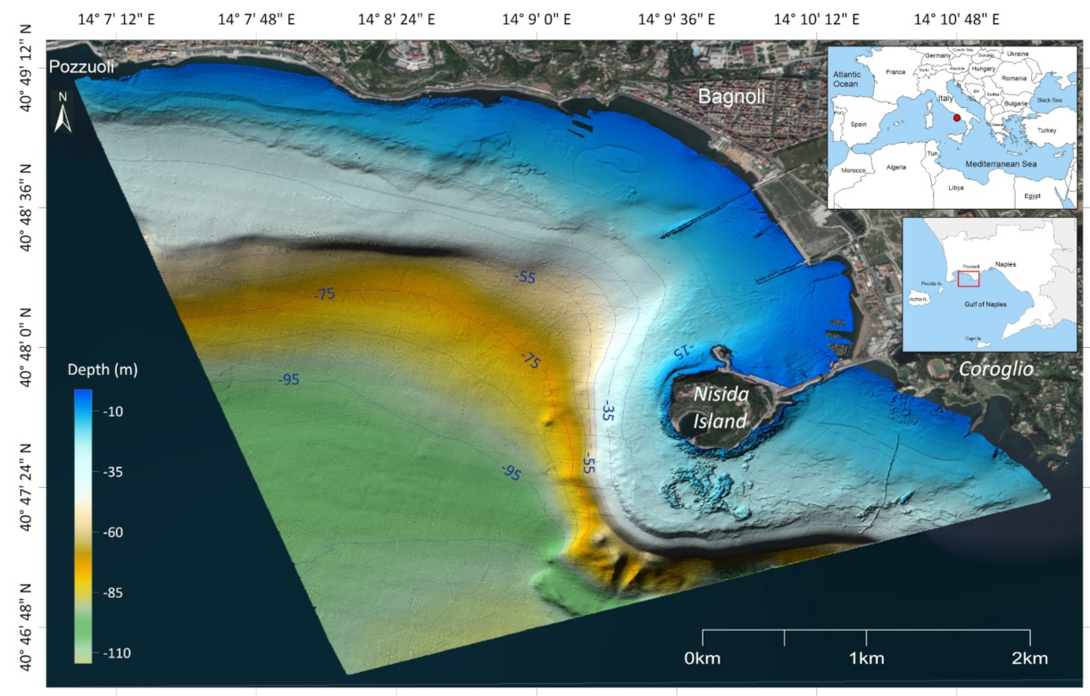
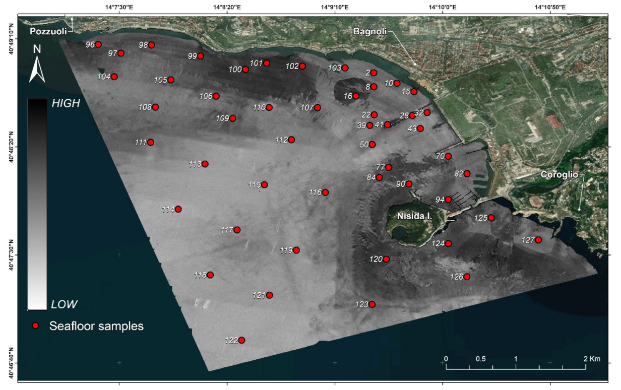
2.1.1. Bagnoli-Corogolio Calibration Area

The data acquisition of this study area was carried out in 2017 by CNR–ISMAR Naples (formerly CNR–IAMC), within the framework of the ABBaCo Project (Italian project ‘Restauro Ambientale e Balneabilità del SIN Bagnoli–Coroglio’—pilot experiments for the environmental restoration and bathing possibility of the Bagnoli–Coroglio coastal area) coordinated by the SZN-Anthon Dohrn, Naples. The project was designed to produce new approaches addressing the remediation of contaminated sites and restoration of marine habitats [66,69]. The study area (Figure 1) was located in the eastern Gulf of Pozzuoli (Naples, southern Italy) and is an integral component of the Campi Flegrei volcanic system, located in the Campania region [66].
The marine area of the Bagnoli coastal zone is part of the caldera collapse that originated from the eruption of the Neapolitan Yellow tuff [70]. The infralittoral setting is characterized by relatively coarse-grained sediments, mainly sand and silty–sand, representing the grain size distribution in equilibrium with a shallow–water, high-energy environment. The sediment constituents are mainly formed by bioclasts and volcaniclasts with a sandy–silt matrix that becomes more abundant towards the distal sector of the gulf [65]. The Bagnoli area has undergone intense industrial activity during most of the last century, from the 1910s until the 1990s. Human-related activities altered the original morphology of the coast, e.g., for the construction of infrastructures on both land and at sea. Steel production ultimately ended in 1990, and the industrial facilities were completely dismantled in the early 2000s [70]. Since then, a series of surveys were carried out with the aim of providing a characterization of soil on land and marine sediments offshore, addressed to the environmental recovery of the area (e.g., [11,13,71,72]). With the ABBaCo project, new results were obtained aimed at the acquisition of new and updated data [8,65,66,73,74,75,76]. Similarly, a high-resolution shaded image derived from bathymetric data (Figure 1) and acoustic mosaic from backscatter data (Figure 2) were obtained, covering about 16 km2 in a water depth range of 1.5–115 m bsl.
The inner shelf is characterized by the presence of stepped terraced surfaces located, in the western sector, at water depths of 10, 25, and 35 m, S-SW oriented. These terraces are expressions of erosional features or toplap/offlap surfaces of local prograding wedges and are likely the result of the dynamic equilibrium between seafloor erosion at the base of storm waves and the sediment supply from the coastline during the Holocene sea-level rise [77]. Stepped terraced surfaces, mainly W oriented, are also present around Nisida island, where the morphology displays a rugged seafloor with a gentle slope (<1°) within 30 m of depth. Two slope breaks bound the island (~10° at 30 m depth and ~15° at 45 m), connecting the inner continental shelf to the deeper part of the bay (see Figure 4 in [66]).
During the ABBaCo project, 50 grab samples were collected and processed for sedimentological and grain-size analysis. The gravel/sand fraction (4000−0.063 mm) was analysed using dry sieving at phi interval, while the fine-grained fraction (0.063−0.0040 mm) was processed with a SYMPATEC laser particle size analyzer [74].

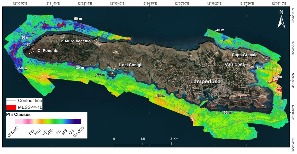
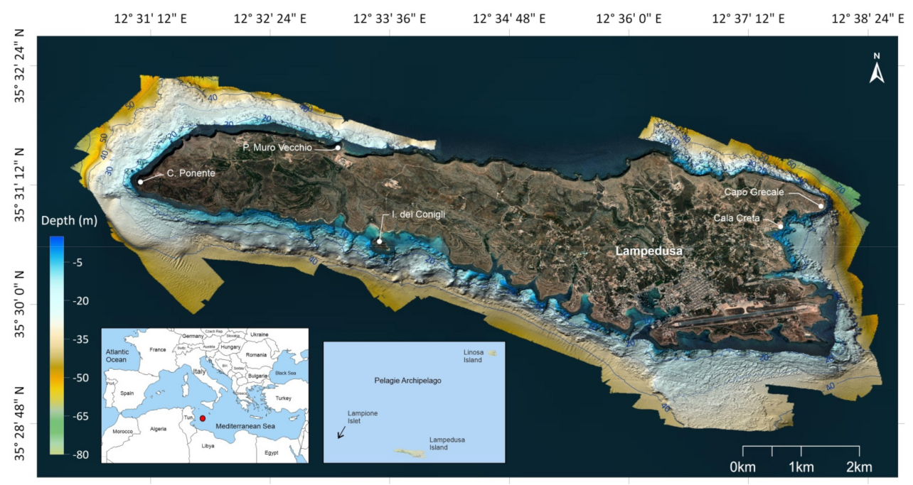
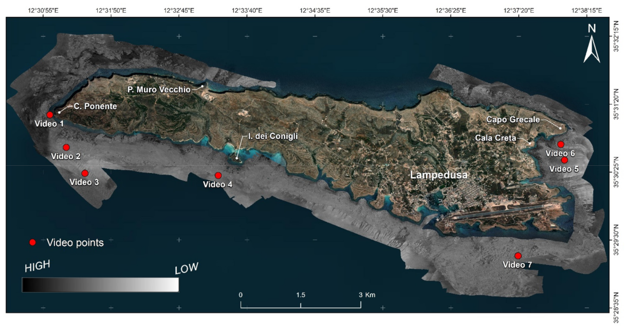
2.1.2. Lampedusa Test Area

Lampedusa is the largest island of the Pelagie Archipelago, followed by Linosa island and the Lampione islet (Sicily, Italy; Figure 3). The island is located in the southern Mediterranean Sea, inside the Sicily Channel, arising from the northern edge of the African continental plate [78,79].
The island (surface area 20 km2; maximum elevation 133 m asl) shows a sub-planar surface inclined toward the south-west and is carved by deep valleys that connect with the narrow inlets along the coast. The island displays rocky cliffs up to 120 m high, which outline a rugged coastline, with tens of rocky highs at a short distance from the coast, mostly occurring along the north-western sector [79,80]. The Lampedusa shoreline can be divided into two main sectors: in the north (from Capo Ponente to Capo Grecale) they are indented, with dominant coastal features varying from steep to sub-vertical cliffs, along with small promontories and bays. In the south, the coast gradually slopes down and includes pocket beaches in the coves. A geophysical survey of Lampedusa was carried out in 2015 by CNR–ISMAR Napoli (formerly CNR–IAMC), within the framework of the project “CAmBiA—Contabilità Ambientale e Bilancio Ambientale” to assess the conservation status and map the distribution of Posidonia oceanica (L.) Delile (Potamogetonaceae) meadows. The aim of the survey was the characterization of the seabed of Lampedusa Island with MBES (both for bathymetric and backscatter data) along with video-camera inspections as ground-truth data (see Figure 3 in [79]) to assess the distribution and the conservation of the P. oceanica meadows. The high-resolution bathymetric map of Lampedusa (depth range of 2–50 m bsl) showed a rugged seafloor all around the island within the first 20–40 m depth, due to extensive rocky outcrops, localized talus deposits and relict morphologies of the seabed, such as P. oceanica meadows on ‘matte’ facies (as defined by [31,79,81]). Locally, vertical scarps 10–20 m high are present, such as in the eastern and northern shallow water sectors. Along the northern coast, the seabed is steeper and dips down to over 50 m bsl (see [79]). Conversely, along the southern sector of the island, the seabed slopes with gradually decreasing gradient in the depth range of 10–50 m. As in Bagnoli, in this study area the snippet data of the MBES was also processed, obtaining an acoustic mosaic at 2.5 m resolution (Figure 4) that was used in [35] for automatic image classification.

2.2. Modeling and Mapping Approach

We used the granulometric distribution values derived from the 50 ground-truth samples collected in Bagnoli to calibrate our model. In detail, the different percentages of sediments belonging to each particle size class (from the coarse to the finest) were used to calculate the mean value of the phi scale using the ‘gran.stats’ function of the ‘rysgran’ package [82]. Phi is a logarithmic parameter for grain size classification whose values range from −9 (i.e., boulders) to 9 (i.e., clay) and is calculated as:
p h i = l o g 2 µ m
The package ‘rysgran’ is based on the size scales adopted by [83,84] while the phi scale was introduced by [85].
We used the values of phi as the dependent variable in our modeling approach using backscatter and depth data as independent variables. In order to take into account the effects of seafloor morphology, slope, aspect, terrain ruggedness index (i.e., TRI), the topographic position index (i.e., TPI), and roughness were computed from the depth data using the function ‘terrain’ from the package ‘raster’ [86].
The set of independent variables was checked for multicollinearity according to a variance inflation factor (i.e., VIF) using the function ‘vifstep’ in the package ‘usdm’ [87]. Specifically, we dropped all variables with VIF ≥ 5 as a threshold indicator of multicollinearity among predictors [88].
The remaining predictors were used in a linear regression model using phi as the dependent variable. We used a backward model selection using function ‘drop1’ in package ‘stats’ [89], recursively dropping all non-significant predictors. The remaining predictors were further sub-selected according to the Akaike information criterion (i.e., AIC) using the function ‘stepAIC’ in the package ‘MASS’ [90]. The AIC is routinely adopted in model selection applications, as the optimal model can be identified according to the lowest value of AIC [91]. Final models’ goodness-of-fit was evaluated calculating the adjusted coefficient of determination (R2adj.). Moreover, predictive performance of the best models was assessed through a 10-fold cross-validation approach, which was repeated five times using the function ‘train’ in the package ‘caret’ [92]. At each cross-validation run, we calculated the values of the predictive coefficient of determination (R2pred.) and root-mean-square error (RMSE), then averaging the results. The residuals from the best model according to the aforementioned criteria were inspected to assess possible violations of the linear regression assumptions. We also took into consideration the possible presence of spatial autocorrelation in the model residuals, which we tested using the function ‘correlog’ in the package ‘ncf’ [93], using 5 m increments for the uniformly distributed distance classes and 1000 permutations to assess the level of significance.
The model was used to produce a 2.5 m resolution map for phi values over the Bagnoli area and was also projected onto a test area (i.e., Lampedusa) where ground-truth data were not available. The final maps were produced by projecting the best regression model on both Bagnoli and Lampedusa areas, also filtering all those pixels reporting phi values >9 and <−9, which could result from minor anomalies in either the backscatter or the depth data. In order to render a more homogenous final map, we computed mean values for each pixel using a moving window approach by a 5 × 5 mean filter, using thefunction ‘focal’ in the package ‘raster’ [86].
In both study areas, we evaluated whether the models were extrapolated beyond the calibration range by means of multivariate environmental similarity surface (i.e., MESS), using the function ‘mess’ in the package ‘dismo’ [94]. In detail, we highlighted in the final output all those areas which had MESS ≤ −10, which can be considered areas of strict extrapolation [95].
Finally, we performed a sensitivity analysis to establish how many ground-truth samples would be needed in order to calibrate and/or validate the model outputs when applied to other areas beside the ones we studied. In order to do so, we took random subsamples from our original dataset, each with increasing sample size compared to the original one (i.e., from 10% to 90% of our original 50 ground-truth data). For each subsample, we recalibrated the model and compared the coefficients to the full model. Each subsample was randomly repeated 50 times. All statistical analyses were performed using R 4.1.2 [89].

3. Results

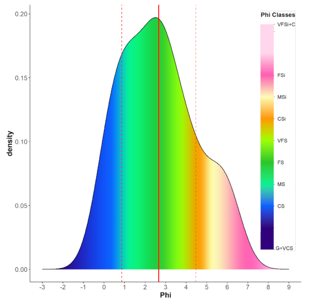
3.1. Ground-Truth Grain Size Classification from Bagnoli–Coroglio

The results from the grain size classification analyses are presented in supplementary material Table S1. The majority of the samples could be generally classified as sand (76%), ranging from very coarse sand (i.e., CS, 2%) to very fine sand (i.e., VFS, 14%). The remainder of the samples (24%) could be classified as silt, ranging from coarse silt (i.e., CSi, 10%) to fine silt (i.e., FSi, 6%). In terms of phi, the computed mean values showed an average of 2.67 ± 1.80 standard deviations. The whole distribution of phi values used for the model calibration can be seen in Figure 5.

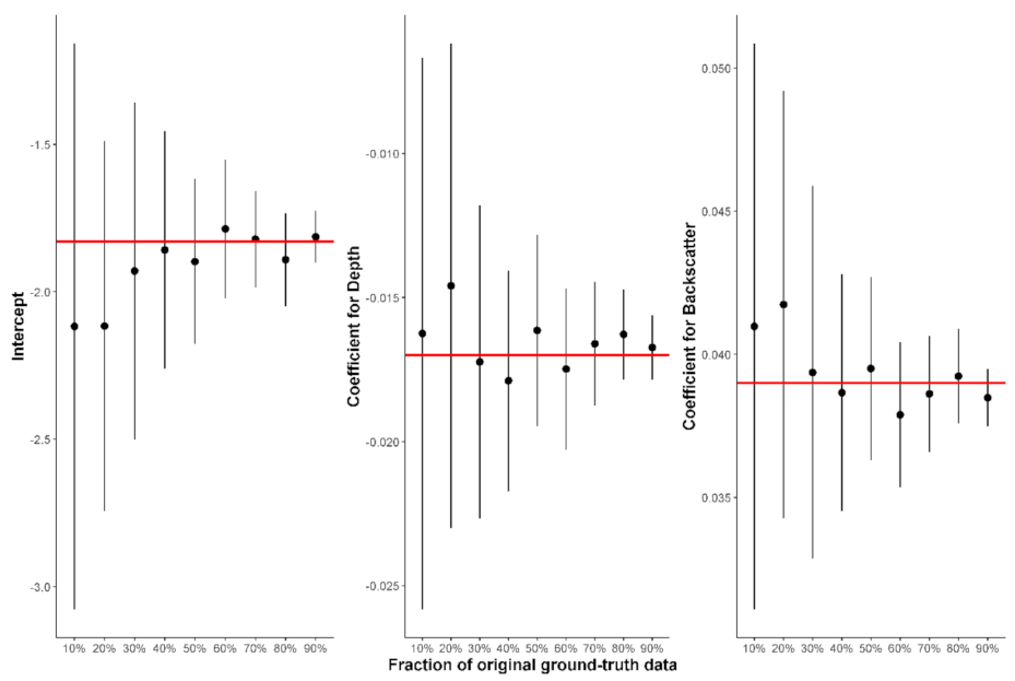
3.2. Model Calibration

After checking for multicollinearity among independent variables, we were left with a set of five covariates, i.e., depth, backscatter, aspect, TPI, and roughness. Starting from a full model, we recursively dropped all non-significant predictors until we were left with only depth and backscatter as significant covariates. In addition, these two variables were included in the best model after backward AIC selection. The final model achieved a high goodness-of-fit, reporting a R2adj.= 0.858, also showing excellent predictive performances (i.e., R2pred.= 0.865 and RMSE = 0.647, Table 1). The statistical analyses showed that both depth and backscatter were excellent predictors for phi, albeit backscatter remarkably outperformed depth when the covariates were considered singularly (Table 1). The final model showed no deviation from linear regression assumptions in the residuals. Spatial autocorrelation was negligible, with a mean value of Moran’s I of −0.027 and only 10% of 633 distance classes results significant (p < 0.05).

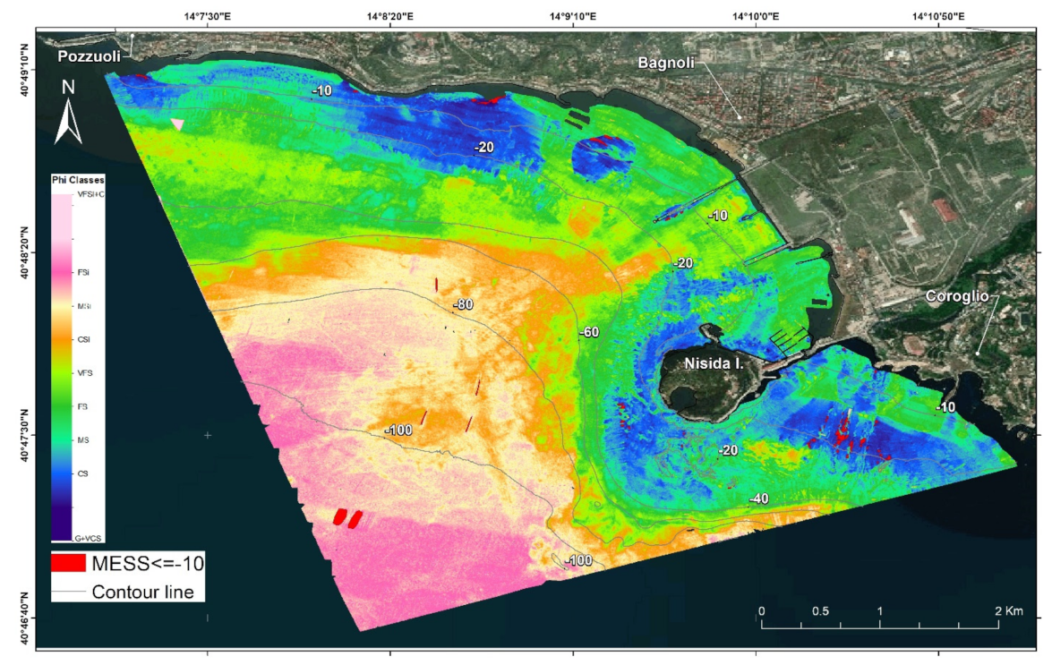
3.3. Final Maps for Bagnoli and Lampedusa

The final maps for Bagnoli and Lampedusa are shown in Figure 6 and Figure 7, respectively. For Bagnoli, only 0.33% of the total pixels in the image could be considered as strictly extrapolated according to MESS analysis, while in Lampedusa the corresponding figure was 1.28%. The mean value of phi for the overall predicted area of Bagnoli was 3.57 ± 1.91, while for Lampedusa the value was 2.84 ± 1.17.
The results from the sensitivity analysis can be seen in Figure 8. The results showed that, even with a sample size as low as 40% of our original dataset, all model parameters (i.e., intercept and coefficients for depth and backscatter) converged on the results of the full model, albeit with some variability resulting from the 50 random replicates with each subsample. Thus, considering that the area of Bagnoli was 16 km2 and that we took 50 ground-truth samples, we could have reached similar results with only 20 ground-truth samples. Consequently, 1.3 ground-truth samples per km2 would be a viable trade-off for validating and/or calibrating our modeling approach in other areas. Accordingly, for the area of Lampedusa, for instance, the results from our model could be validated by 24 ground-truth samples, as the overall surveyed area was approximately 18 km2.

4. Discussion

4.1. Bagnoli–Coroglio Calibration Area

In the Bagnoli–Coroglio area, the seafloor map showed good correspondence with the sedimentological map preliminarily recognized by expert-based interpretation of the backscatter mosaic published in [65]. The coarse-grained sediments were concentrated in two sectors: the area between Pozzuoli and Bagnoli and the southern sector of the Bagnoli–Coroglio offshore, including Nisida island and the area at its south. In particular, the northern sector was characterized by relatively high acoustic reflection (Figure 2) that corresponded to “gravelly coarse sand” in [65]. These sediments were mostly concentrated in two areas, one below a slide deposit that contributes a supply of coarse material from the coast, and the other corresponding to a sub-circular depression about 0.1 km2 wide where coarse sand settled. Such depression was described in more detail by [8]. Figure 6 showed the same gravelly coarse sand distribution (blue area), both from north and south sectors, and also showed coarse sand entrapped by bottom currents near the piers of the disused industrial site of Bagnoli [8].
In the southern part of the first study area, offshore of the Coroglio tuffaceous cliff, a series of morphologic depressions and ridges have favored a current-driven separation between the coarse deposits (depressions) from the fine-grained material (ridges), as shown by [8]. These morphological structures are clearly visible in Figure 6, supporting the outputs of the applied method. The central part of the study area, off the pier of the former industrial site, was classified as fine sand/very fine sand in [65], based on both backscatter values and seafloor sampling. Nevertheless, the acoustic mosaic showed some patches of intermediate to high backscatter, likely due to the occurrence of coarser shallow water deposits, which would be hard to discriminate visually by an expert. In this specific case, the seafloor map differs from that of [65], because the modeling approach presented here was able to recognize the heterogeneous distribution of medium sand to fine sand, with a predominance of the latter. In contrast, expert-based classification, or even automatic image classifications, might coerce aggregations or render sharp boundaries between the facies, preventing the realization of a more realistic distribution between the granulometric classes. Thus, even when close to reality, polygon classification can be limited in terms of resolution and detail compared to the outputs produced in this study. The same can be said for silty sediments, as this classification creates the possibility of distinguishing between coarse silt to very fine silt, avoiding creating a single class of silt and clay, as was done in [65]. Silt and clay were detected in the south-western distal part of the study area corresponding to the Bagnoli Valley [77], a morphostructural depression connecting the Bagnoli foreshore with the outer continental shelf of Pozzuoli Bay, which delivers coastal sediments towards deep water areas. In [66], a flow analysis, based on seafloor morphology data, was carried out to derive the stream paths towards the Valley, that showed a preferential direction of the sediment transport that fits with what is shown in Figure 6.
Finally, the presence of bedrock in the southern sector of Nisida island was recognized by experts from the morphology data published in [65]. In this sector, linear regression classified this sub-outcropping structure as an alternation of fine sand and coarse sand. Admittedly, as there were no grabs done in this sector and considering that the model was calibrated on loose sediments, rocky outcrops or very large boulders could have been misidentified.
Yet, the MESS sectors of the Bagnoli study area were only 0.33% of the total pixels and, analysing the map, they corresponded mostly to backscatter noise or to coarser sediments, which were underrepresented in the calibration data and might have led to strict extrapolation in some minor parts of the map.

4.2. Lampedusa Island Test Area

The sediment distribution map obtained from the linear regression model for Lampedusa, where no ground-truth was available, is in concordance with the classification carried out in [35]. In the latter study, a preliminary benthoscape classification of the island was carried out with the use of remote sensing object-based image analysis (RSOBIA), that segmented and classified the acoustic mosaic obtained from snippet data processing [96]. The map in [35] was presented as preliminary because no grab sampling was available and the seabed was mainly classified only by experts based on its acoustics facies pattern (i.e., fine sediments exhibiting low backscatter, and coarse sediments corresponding to high backscatter), and the results of RSOBIA segmentation. In general, the seafloor map produced here by the model was characterized mostly by fine sand, representing the predominant grain size. In detail, the southern sector of the island was mostly characterized by a distribution of fine and very fine sand, with channels of medium coarse sand. Posidonia oceanica meadows were identified with video-inspections and added in benthoscape classification as overprint layers [35,79]. Well-developed meadows of this plant cause a decrease in the backscatter values, shifting the classification toward fine sands, as already shown in [31]. So, in the case of meadows or any other plant-dominated seafloors, visual inspections or scuba diving as ground-truth information can outperform the linear modeling approach. The sediment distribution of the southern flank showed a classic depositional model of coastal environments, with the onshore coarse grain-size (blue areas in Figure 7) and finer material offshore. Coarser sand was present along the coastline and in all north-western sectors of Lampedusa, i.e., from Capo Ponente to P. Muro Vecchio. As shown by ROV images (see Video 1 in Figure 4 published in [35,79]), very coarse heterogeneous materials (well-rounded pebbles and boulders) in poorly sorted calcareous gravels were detected, forming a terraced surface at the foot of the submerged cliffs. This formation was interpreted as a foot-cliff deposit generated by the wave-related winnowing of talus, likely derived by progressive cliff failures [97]. As already showed for the Bagnoli–Coroglio site, rocky outcrops can be misclassified by the linear regression model, due to underrepresentation in the calibration ground-truth data.
Accordingly, the MESS areas were more present in sectors with higher reflectivity, as for Bagnoli, because there were no calibration samples for this class. The same reasoning can be followed for very fine sediments, such as clay without silt (e.g., Cala Creta in Figure 4 and Figure 7), which were also underrepresented in the calibration data from Bagnoli–Coroglio, where the finest sediments were very fine silt grouped with clay. Admittedly, the linear model predictions in the Lampedusa area need to be validated by grab samples that, according to our sensitivity analysis, could be as few as 24 samples.

4.3. Comparisons with Other Approaches

Supervised methods for seafloor grain size and/or habitat classification based on remote sensing data have been shown to provide accurate results, especially when paired with robust ground-truth sampling [21,27,98]. Yet, several supervised approaches resulted in comparatively low accuracy and high error rates when dealing with a morphologically simple seabed characterized by a high sedimentary complexity [30]. Despite state-of-the-art statistical approaches, such low map accuracy could be attributed to an inadequate classification system, low discriminatory power of the available predictors, and the spatial complexity of the survey site compared to the positioning accuracy of the grab samples [30]. Our approach can be seen as different and innovative compared to other studies, as it used a quantitative model for the spatial distribution of sediment fractions, which did not oversimplify the final output into a few categories. On the contrary, as the final model outputs a map for phi values, it can be seen as an extremely detailed map that clearly shows gradients and boundaries among sediments, allowing for more precise habitat mapping or geological study of the seafloor in coastal environments. Such a detailed map can be easily transformed into a simpler map of substrate types, as for instance those defined by the European Nature Information System (EUNIS) hierarchical classification [99] or other marine habitat classification schemes [61]
After cross-validation, our model showed excellent predictive performance (R2pred. = 0.865). Such a level of accuracy exceeds an 85% target accuracy that has usually been considered ideal for thematic mapping based on remotely sensed data [100]. Such a level of accuracy can be surpassed by other modeling approaches, such as fully connected conditional random field [101], but this model was calibrated on a few substrate classes rather than a continuous variable, such as phi.
Another typical classification model for seafloor data based on MBES is random forest [27,102,103,104]. This type of model has been shown to offer accuracy as high as 83% [103]. Moreover, when applied to seafloor data, random forest is used as a classification approach for few categories, such as those proposed by EUNIS, showing limitations and underperformance when substrate complexity is present [30]. Admittedly, random forest regression for continuous data is widely used in ecological research [105,106], yet, in continental shelf research, random forest is mostly used as a supervised classification approach, although there are recent examples where it has been employed for continuous modeling [18,62,63].
Other statistical methods rely on the use of proprietary software compared to free software, such as R or QGIS. Some approaches rely on object-based image analysis, for example, RSOBIA, which is implemented in ArcGIS [30,35,96,107]. The segmentation implemented in RSOBIA requires the user to define both the number and the minimum size of the clusters, which are then classified by a k-means clustering approach. Another ArcGIS tool is Terrain Attribute Selection for Spatial Ecology [108], which derives six variables from bathymetry that can be used along with backscatter data in a multiresolution segmentation algorithm requiring expert judgment to define scale and input variables. Both the aforementioned approaches in ArcGIS can offer good predictive performance, but they require proprietary software, some degree of expert handling for fine tuning the model and, finally, they both suffer from the same problems as random forest when dealing with complex seafloors [30].
Other approaches to seafloor mapping have been applied as well, including both expert-based and supervised classification. The authors of [109] focused on soft-sediment physical features to delineate distinct acoustic facies that presumably represented different lithological types of seabed sediments. The different facies were defined in ArcGIS according to similar backscatter characteristics, which were later validated by sediment samples analysed for particle size.
In [110], the applicability of supervised learning techniques for benthic habitat characterization using angular backscatter response was demonstrated. The study involved characterization of acoustic backscatter data from multibeam systems, using four different supervised learning methods to generate benthic habitat maps.
In [5], the authors combined a suite of geomorphometric and textural analytical techniques to map specific types of seafloor morphologies and compositions. The seabed was classified into five elementary morphological zones, using morphometric derivatives, bathymetric position index and geomorphometric mapping, to produce morphologic and seabed composition maps of the predominant habitats. Finally, ref. [111] used ensemble modeling to map seafloor sediment distributions and shifts with minimal ground-truth data combined with hydroacoustic datasets in the Sylt outer reef.

4.4. Limits and Future Developments

Despite several, advantages, our modeling approach was unable to correctly identify rocky outcrops and P. oceanica meadows. The model was also constrained by the calibration data, which was underrepresented in both very fine and very coarse sediments. Moreover, as our survey areas were both limited to shallow water, the model needs to be recalibrated when waters are deeper than 110 m. In its current stage of development, our model is best suited to all those shallow-water areas with loose sediments intermingled with a few hard substrates, regardless of terrain, that can be either smooth or rough [43]. Future developments of the model will be able to detect the presence of consolidated sediments and function in deeper waters by expanding the calibration dataset.

5. Conclusions

The modeling approach presented in this research can be seen as an accurate method for high resolution and continuous mapping of loose sediments in the continental shelf, which can be used in several applications from habitat mapping to substrate shifting when the analysis is repeated across time. The method relies on free software and can be validated and/or recalibrated using 1.3 ground-truth samples per km2 of survey area. The results from the Bagnoli–Coroglio area showed excellent accuracy and negligible areas of extrapolation, while the map for Lampedusa was largely in concordance with expert-based previous seafloor mapping [35,79], although there is a need to validate the results by grab samples. Regardless of these limitations, our modeling approach is a flexible tool whose main advantage is the rendering of a continuous map for sediment size that does not show sharp boundaries or few sediment classes. These features can be pivotal in ecological, geological and management applications in marine coastal ecosystems.

Supplementary Materials

The following supporting information can be downloaded at: https://www.mdpi.com/article/10.3390/rs14051268/s1, Table S1: Results from the granumoletric analyses from the 50 grab samples in the Bagnoli-Coroglio calibration area. The results include the percentages from all granulometric classes (according to Udden & Wentworth) and the corresponding phi values (according to Krumbein).

Author Contributions

Conceptualization, S.I., M.I. and R.T.; methodology, S.I., M.I. and M.D.F.; software, S.I., M.I. and G.D.M.; validation, M.D.F.; formal analysis, S.I. and M.I.; investigation, S.I. and G.D.M.; resources, M.S. and R.T.; data curation, S.I. and M.I.; writing—original draft preparation, S.I. and M.I.; writing—review and editing, M.D.F. and G.D.M.; visualization, S.I. and G.D.M.; supervision, M.S. and R.T.; project administration, M.S. and R.T.; funding acquisition, M.S. and R.T. All authors have read and agreed to the published version of the manuscript.

Funding

This research work has been conducted by ISMAR (formerly IAMC)—CNR Napoli within the framework of the ABBaCo Project (Italian project “Restauro Ambientale e Balneabilità del SIN Bagnoli–Coroglio”—pilot experiments for the environmental restoration and balneability of Bagnoli–Coroglio coastal area) coordinated by Stazione Zoologica Anthon Dohrn Napoli (SNZ-CNR contract n. 2974; Funding Institution MIUR; http://www.szn.it/index.php/en/research/integrative-marine-ecology/research-projects-emi/abbaco, accessed on 1 March 2022). This study also benefited from contribution by the project ‘Implementation of research activity and monitoring around Pelagie Islands Marine Protected Area’, within the project ‘CAmBiA—Contabilità Ambientale e Bilancio Ambientale’ funded by the Ministry for Environment, Land and Sea Protection (also known as MATTM—Ministero dell’Ambiente e della Tutela del Territorio e del Mare), Directive n° 5135 of March 2015. Finally, this study also benefited from contribution by the RITMARE (La Ricerca ITaliana per il MARE—http://www.ritmare.it/, accessed on 1 March 2022) Flagship Project, funded by the Ministry of Education, Universities and Research (also known as MIUR—Ministero dell’Istruzione, dell’Università e della Ricerca) [NRP 2011–2013].

Data Availability Statement

The entire data for the grab samples is available as Supplementary Materials. The raster files for backscatter and depth for both the calibration and test areas can be requested at Sara Innangi [email protected].

Acknowledgments

We thank Simone D’Ippolito, the captain of the M/B ‘Risal’, and Francesco Saggiomo, the captain of Research Catamaran “Idrosfera”.

Conflicts of Interest

The authors declare no conflict of interest.

References

  1. Cusson, M.; Bourget, E. Influence of topographic heterogeneity and spatial scales on the structure of the neighbouring intertidal endobenthic macrofaunal community. Mar. Ecol. Prog. Ser. 1997, 150, 181–193. [Google Scholar] [CrossRef] [Green Version]
  2. De Falco, G.; Tonielli, R.; Di Martino, G.; Innangi, S.; Simeone, S.; Parnum, I.M. Relationships between multibeam backscatter, sediment grain size and Posidonia oceanica seagrass distribution. Cont. Shelf Res. 2010, 30, 1941–1950. [Google Scholar] [CrossRef]
  3. Huang, Z.; Siwabessy, J.; Cheng, H.; Nichol, S. Using Multibeam Backscatter Data to Investigate Sediment-Acoustic Relationships. J. Geophys. Res. Ocean 2018, 123, 4649–4665. [Google Scholar] [CrossRef]
  4. Kostylev, V.; Todd, B.; Fader, G.; Courtney, R.; Cameron, G.; Pickrill, R. Benthic habitat mapping on the Scotian Shelf based on multibeam bathymetry, surficial geology and sea floor photographs. Mar. Ecol. Prog. Ser. 2001, 219, 121–137. [Google Scholar] [CrossRef] [Green Version]
  5. Micallef, A.; Le Bas, T.P.; Huvenne, V.A.I.; Blondel, P.; Hühnerbach, V.; Deidun, A. A multi-method approach for benthic habitat mapping of shallow coastal areas with high-resolution multibeam data. Cont. Shelf Res. 2012, 39–40, 14–26. [Google Scholar] [CrossRef] [Green Version]
  6. Orpin, A.R.; Kostylev, V.E. Towards a statistically valid method of textural sea floor characterization of benthic habitats. Mar. Geol. 2006, 225, 209–222. [Google Scholar] [CrossRef]
  7. Snelgrove, P.V.R.; Butman, C.A. Animal Sediment Relationships Revisited—Cause versus Effect. Oceanogr. Lit. Rev. 1995, 8, 668. [Google Scholar]
  8. Di Martino, G.; Innangi, S.; Sacchi, M.; Tonielli, R. Seafloor morphology changes in the inner-shelf area of the Pozzuoli Bay, Eastern Tyrrhenian Sea. Mar. Geophys. Res. 2021, 42, 13. [Google Scholar] [CrossRef]
  9. Siwabessy, P.J.W.; Tran, M.; Picard, K.; Brooke, B.P.; Huang, Z.; Smit, N.; Williams, D.K.; Nicholas, W.A.; Nichol, S.L.; Atkinson, I. Modelling the distribution of hard seabed using calibrated multibeam acoustic backscatter data in a tropical, macrotidal embayment: Darwin Harbour, Australia. Mar. Geophys. Res. 2018, 39, 249–269. [Google Scholar] [CrossRef]
  10. Lathrop, R.G.; Cole, M.; Senyk, N.; Butman, B. Seafloor habitat mapping of the New York Bight incorporating sidescan sonar data. Estuar. Coast. Shelf Sci. 2006, 68, 221–230. [Google Scholar] [CrossRef]
  11. Albanese, S.; De Vivo, B.; Lima, A.; Cicchella, D.; Civitillo, D.; Cosenza, A. Geochemical baselines and risk assessment of the Bagnoli brownfield site coastal sea sediments (Naples, Italy). J. Geochem. Explor. 2010, 105, 19–33. [Google Scholar] [CrossRef]
  12. Sprovieri, M.; Barra, M.; Del Core, M.; Di Martino, G.; Giaramita, L.; Gherardi, S.; Innangi, S.; Oliveri, E.; Passaro, S.; Romeo, T.; et al. Marine Pollution from Shipwrecks at the Sea Bottom: A Case Study from the Mediterranean Basin. In Mediterranean Sea, Ecosystems, Economic Importance and Environmental Threats; Hughes, T.B., Ed.; NOVA Science Publisher, Inc.: Hauppauge, NY, USA, 2013; pp. 35–64. ISBN 978-1-62618-238-7. [Google Scholar]
  13. Adamo, P.; Arienzo, M.; Bianco, M.R.; Terribile, F.; Violante, P. Heavy metal contamination of the soils used for stocking raw materials in the former ILVA iron-steel industrial plant of Bagnoli (southern Italy). Sci. Total Environ. 2002, 295, 17–34. [Google Scholar] [CrossRef]
  14. Trifuoggi, M.; Donadio, C.; Mangoni, O.; Ferrara, L.; Bolinesi, F.; Nastro, R.A.; Stanislao, C.; Toscanesi, M.; Di Natale, G.; Arienzo, M. Distribution and enrichment of trace metals in surface marine sediments in the Gulf of Pozzuoli and off the coast of the brownfield metallurgical site of Ilva of Bagnoli (Campania, Italy). Mar. Pollut. Bull. 2017, 124, 502–511. [Google Scholar] [CrossRef] [PubMed]
  15. Snellen, M.; Gaida, T.C.; Koop, L.; Alevizos, E.; Simons, D.G. Performance of Multibeam Echosounder Backscatter-Based Classification for Monitoring Sediment Distributions Using Multitemporal Large-Scale Ocean Data Sets. IEEE J. Ocean. Eng. 2019, 44, 142–155. [Google Scholar] [CrossRef] [Green Version]
  16. Misiuk, B.; Lecours, V.; Bell, T. A multiscale approach to mapping seabed sediments. PLoS ONE 2018, 13, e0193647. [Google Scholar] [CrossRef] [Green Version]
  17. Pydyn, A.; Popek, M.; Kubacka, M.; Janowski, Ł. Exploration and reconstruction of a medieval harbour using hydroacoustics, 3-D shallow seismic and underwater photogrammetry: A case study from Puck, southern Baltic Sea. Archaeol. Prospect. 2021, 28, 527–542. [Google Scholar] [CrossRef]
  18. Montereale Gavazzi, G.; Kapasakali, D.A.; Kerchof, F.; Deleu, S.; Degraer, S.; Van Lancker, V. Subtidal Natural Hard Substrate Quantitative Habitat Mapping: Interlinking Underwater Acoustics and Optical Imagery with Machine Learning. Remote Sens. 2021, 13, 4608. [Google Scholar] [CrossRef]
  19. Todd, B.J.; Fader, G.B.J.; Courtney, R.C.; Pickrill, R.A. Quaternary geology and surficial sediment processes, Browns Bank, Scotian Shelf, based on multibeam bathymetry. Mar. Geol. 1999, 162, 165–214. [Google Scholar] [CrossRef]
  20. Innangi, S.; Passaro, S.; Tonielli, R.; Milano, G.; Ventura, G.; Tamburrino, S. Seafloor mapping using high-resolution multibeam backscatter: The Palinuro Seamount (Eastern Tyrrhenian Sea). J. Maps 2016, 12, 736–746. [Google Scholar] [CrossRef] [Green Version]
  21. Stephens, D.; Diesing, M. A comparison of supervised classification methods for the prediction of substrate type using multibeam acoustic and legacy grain-size data. PLoS ONE 2014, 9, e93950. [Google Scholar] [CrossRef]
  22. Hasan, R.C.; Ierodiaconou, D.; Monk, J. Evaluation of Four Supervised Learning Methods for Benthic Habitat Mapping Using Backscatter from Multi-Beam Sonar. Remote Sens. 2012, 4, 3427–3443. [Google Scholar] [CrossRef] [Green Version]
  23. Lucieer, V.; Lamarche, G. Unsupervised fuzzy classification and object-based image analysis of multibeam data to map deep water substrates, Cook Strait, New Zealand. Cont. Shelf Res. 2011, 31, 1236–1247. [Google Scholar] [CrossRef]
  24. Blondel, P.; Gòmez Sichi, O. Textural analyses of multibeam sonar imagery from Stanton Banks, Northern Ireland continental shelf. Appl. Acoust. 2009, 70, 1288–1297. [Google Scholar] [CrossRef]
  25. Biondo, M.; Bartholomä, A. A multivariate analytical method to characterize sediment attributes from high-frequency acoustic backscatter and ground-truthing data (Jade Bay, German North Sea coast). Cont. Shelf Res. 2017, 138, 65–80. [Google Scholar] [CrossRef]
  26. Dartnell, P.; Gardner, J.V. Predicting seafloor facies from multibeam bathymetry and backscatter data. Photogramm. Eng. Remote Sens. 2004, 70, 1081–1091. [Google Scholar] [CrossRef] [Green Version]
  27. Diesing, M.; Green, S.L.; Stephens, D.; Lark, R.M.; Stewart, H.A.; Dove, D. Mapping seabed sediments: Comparison of manual, geostatistical, object-based image analysis and machine learning approaches. Cont. Shelf Res. 2014, 84, 107–119. [Google Scholar] [CrossRef] [Green Version]
  28. Janowski, L.; Madricardo, F.; Fogarin, S.; Kruss, A.; Molinaroli, E.; Kubowicz-Grajewska, A.; Tegowski, J. Spatial and temporal changes of tidal inlet using object-based image analysis of multibeam echosounder measurements: A case from the Lagoon of Venice, Italy. Remote Sens. 2020, 12, 2117. [Google Scholar] [CrossRef]
  29. Pillay, T.; Cawthra, H.C.; Lombard, A.T. Characterisation of seafloor substrate using advanced processing of multibeam bathymetry, backscatter, and sidescan sonar in Table Bay, South Africa. Mar. Geol. 2020, 429, 106332. [Google Scholar] [CrossRef]
  30. Diesing, M.; Mitchell, P.J.; O’Keeffe, E.; Montereale Gavazzi, G.; Le Bas, T. Limitations of Predicting Substrate Classes on a Sedimentary Complex but Morphologically Simple Seabed. Remote Sens. 2020, 12, 3398. [Google Scholar] [CrossRef]
  31. Innangi, S.; Barra, M.; Di Martino, G.; Parnum, I.M.; Tonielli, R.; Mazzola, S. Reson SeaBat 8125 backscatter data as a tool for seabed characterization (Central Mediterranean, Southern Italy): Results from different processing approaches. Appl. Acoust. 2015, 87, 109–122. [Google Scholar] [CrossRef]
  32. Erdey-Heydorn, M.D. An ArcGIS seabed characterization toolbox developed for investigating benthic habitats. Mar. Geod. 2008, 31, 318–358. [Google Scholar] [CrossRef]
  33. Huang, Z.; Siwabessy, J.; Nichol, S.L.; Brooke, B.P. Predictive mapping of seabed substrata using high-resolution multibeam sonar data: A case study from a shelf with complex geomorphology. Mar. Geol. 2014, 357, 37–52. [Google Scholar] [CrossRef]
  34. Ierodiaconou, D.; Schimel, A.C.G.; Kennedy, D.; Monk, J.; Gayland, G.; Young, M.; Diesing, M.; Rattray, A. Combining pixel and object based image analysis of ultra-high resolution multibeam bathymetry and backscatter for habitat mapping in shallow marine waters. Mar. Geophys. Res. 2018, 39, 271–288. [Google Scholar] [CrossRef]
  35. Innangi, S.; Tonielli, R.; Romagnoli, C.; Budillon, F.; Di Martino, G.; Innangi, M.; Laterza, R.; Le Bas, T.; Lo Iacono, C. Seabed mapping in the Pelagie Islands marine protected area (Sicily Channel, southern Mediterranean) using Remote Sensing Object Based Image Analysis (RSOBIA). Mar. Geophys. Res. 2019, 40, 333–355. [Google Scholar] [CrossRef] [Green Version]
  36. Innangi, S.; Di Martino, G.; Romagnoli, C.; Tonielli, R. Seabed classification around Lampione islet, Pelagie Islands Marine Protected area, Sicily Channel, Mediterranean Sea. J. Maps 2019, 15, 153–164. [Google Scholar] [CrossRef]
  37. Lacharité, M.; Brown, C.J.; Gazzola, V. Multisource multibeam backscatter data: Developing a strategy for the production of benthic habitat maps using semi-automated seafloor classification methods. Mar. Geophys. Res. 2018, 39, 307–322. [Google Scholar] [CrossRef]
  38. Marsh, I.; Brown, C. Neural network classification of multibeam backscatter and bathymetry data from Stanton Bank (Area IV). Appl. Acoust. 2009, 70, 1269–1276. [Google Scholar] [CrossRef]
  39. Zelada Leon, A.; Huvenne, V.A.I.; Benoist, N.M.A.; Ferguson, M.; Bett, B.J.; Wynn, R.B. Assessing the Repeatability of Automated Seafloor Classification Algorithms, with Application in Marine Protected Area Monitoring. Remote Sens. 2020, 12, 1572. [Google Scholar] [CrossRef]
  40. Fonseca, L.; Mayer, L. Remote estimation of surficial seafloor properties through the application Angular Range Analysis to multibeam sonar data. Mar. Geophys. Res. 2007, 28, 119–126. [Google Scholar] [CrossRef]
  41. Lucieer, V.; Roche, M.; Degrendele, K.; Malik, M.; Dolan, M.; Lamarche, G. User expectations for multibeam echo sounders backscatter strength data-looking back into the future. Mar. Geophys. Res. 2018, 39, 23–40. [Google Scholar] [CrossRef]
  42. Innangi, S.; Barra, M.; Brando, A.; Coppa, S.; Di Martino, G.; Guala, I.; Ferraro, L.; Tonielli, R. Construction of the thematic maps of the seabed along the Lucanian Tyrrhenian Coast of Maratea (PZ). Rend. Online Soc. Geol. Ital. 2008, 3, 476–477. [Google Scholar]
  43. Kloser, R.J.; Penrose, J.D.; Butler, A.J. Multi-beam backscatter measurements used to infer seabed habitats. Cont. Shelf Res. 2010, 30, 1772–1782. [Google Scholar] [CrossRef]
  44. Briggs, K.B.; Tang, D.; Williams, K.L. Characterization of interface roughness of rippled sand off fort Walton Beach, Florida. IEEE J. Ocean. Eng. 2002, 27, 505–514. [Google Scholar] [CrossRef]
  45. Fonseca, L.; Brown, C.; Calder, B.; Mayer, L.; Rzhanov, Y. Angular range analysis of acoustic themes from Stanton Banks Ireland: A link between visual interpretation and multibeam echosounder angular signatures. Appl. Acoust. 2009, 70, 1298–1304. [Google Scholar] [CrossRef]
  46. Pinson, S.; Stéphan, Y.; Holland, C.W. Roughness parameters imaging with a multibeam echosounder. J. Acoust. Soc. Am. 2017, 141, 3532. [Google Scholar] [CrossRef]
  47. Ferrini, V.L.; Flood, R.D. The effects of fine-scale surface roughness and grain size on 300 kHz multibeam backscatter intensity in sandy marine sedimentary environments. Mar. Geol. 2006, 228, 153–172. [Google Scholar] [CrossRef]
  48. Lo Iacono, C.; Grinyó, J.; Conlon, S.; Lafosse, M.; Rabaute, A.; Pierdomenico, M.; Perea, H.; d’Acremont, E.; Gràcia, E. Chapter 55—Near-pristine benthic habitats on the Francesc Pagès Bank, Alboran Sea, western Mediterranean. In Seafloor Geomorphology as Benthic Habitat, 2nd ed.; Harris, P.T., Baker, E., Eds.; Elsevier: Amsterdam, The Netherlands, 2020; pp. 889–901. ISBN 978-0-12-814960-7. [Google Scholar]
  49. Lo Iacono, C.; Gràcia, E.; Diez, S.; Bozzano, G.; Moreno, X.; Dañobeitia, J.; Alonso, B. Seafloor characterization and backscatter variability of the Almería Margin (Alboran Sea, SW Mediterranean) based on high-resolution acoustic data. Mar. Geol. 2008, 250, 1–18. [Google Scholar] [CrossRef]
  50. Simons, D.G.; Snellen, M. A Bayesian approach to seafloor classification using multi-beam echo-sounder backscatter data. Appl. Acoust. 2009, 70, 1258–1268. [Google Scholar] [CrossRef]
  51. De Falco, G.; Conforti, A.; Brambilla, W.; Budillon, F.; Ceccherelli, G.; De Luca, M.; Di Martino, G.; Guala, I.; Innangi, S.; Pascucci, V.; et al. Coralligenous banks along the western and northern continental shelf of Sardinia Island (Mediterranean Sea). J. Maps 2022, 1–10. [Google Scholar] [CrossRef]
  52. Rende, S.F.; Bosman, A.; Di Mento, R.; Bruno, F.; Lagudi, A.; Irving, A.D.; Dattola, L.; Di Giambattista, L.; Lanera, P.; Proietti, R.; et al. Ultra-High-Resolution Mapping of Posidonia oceanica (L.) Delile Meadows through Acoustic, Optical Data and Object-based Image Classification. J. Mar. Sci. Eng. 2020, 8, 647. [Google Scholar] [CrossRef]
  53. Goff, J.A.; Kraft, B.J.; Mayer, L.A.; Schock, S.G.; Sommerfield, C.K.; Olson, H.C.; Gulick, S.P.S.; Nordfjord, S. Seabed characterization on the New Jersey middle and outer shelf: Correlatability and spatial variability of seafloor sediment properties. Mar. Geol. 2004, 209, 147–172. [Google Scholar] [CrossRef]
  54. Sutherland, T.; Galloway, J.; Loschiavo, R.; Levings, C.; Hare, R. Calibration techniques and sampling resolution requirements for groundtruthing multibeam acoustic backscatter (EM3000) and QTC VIEWTM classification technology. Estuar. Coast. Shelf Sci. 2007, 75, 447–458. [Google Scholar] [CrossRef]
  55. Briggs, K. High-Frequency Acoustic Scattering from Sediment Interface Roughness and Volume Inhomogeneities; Naval Research Lab Stennis Space Center: Hancock County, MI, USA, 1994. [Google Scholar]
  56. Hines, P.C. Theoretical model of acoustic backscatter from a smooth seabed. J. Acoust. Soc. Am. 1990, 88, 324. [Google Scholar] [CrossRef]
  57. Stewart, W.K.; Chu, D.; Malik, S.; Lerner, S.; Singh, H. Quantitative seafloor characterization using a bathymetric sidescan sonar. IEEE J. Ocean. Eng. 1994, 19, 599–610. [Google Scholar] [CrossRef]
  58. McGonigle, C.; Collier, J.S. Interlinking backscatter, grain size and benthic community structure. Estuar. Coast. Shelf Sci. 2014, 147, 123–136. [Google Scholar] [CrossRef]
  59. Brown, C.J.; Beaudoin, J.; Brissette, M.; Gazzola, V. Multispectral multibeam echo sounder backscatter as a tool for improved seafloor characterization. Geosciences 2019, 9, 126. [Google Scholar] [CrossRef] [Green Version]
  60. Boswarva, K.; Butters, A.; Fox, C.J.; Howe, J.A.; Narayanaswamy, B. Improving marine habitat mapping using high-resolution acoustic data; a predictive habitat map for the Firth of Lorn, Scotland. Cont. Shelf Res. 2018, 168, 39–47. [Google Scholar] [CrossRef]
  61. Strong, J.A.; Clements, A.; Lillis, H.; Galparsoro, I.; Bildstein, T.; Pesch, R. A review of the influence of marine habitat classification schemes on mapping studies: Inherent assumptions, influence on end products, and suggestions for future developments. ICES J. Mar. Sci. 2019, 76, 10–22. [Google Scholar] [CrossRef] [Green Version]
  62. Misiuk, B.; Brown, C.J.; Robert, K.; Lacharité, M. Harmonizing Multi-Source Sonar Backscatter Datasets for Seabed Mapping Using Bulk Shift Approaches. Remote Sens. 2020, 12, 601. [Google Scholar] [CrossRef] [Green Version]
  63. Misiuk, B.; Diesing, M.; Aitken, A.; Brown, C.J.; Edinger, E.N.; Bell, T. A Spatially Explicit Comparison of Quantitative and Categorical Modelling Approaches for Mapping Seabed Sediments Using Random Forest. Geosciences 2019, 9, 254. [Google Scholar] [CrossRef] [Green Version]
  64. Halpern, B.S.; Walbridge, S.; Selkoe, K.A.; Kappel, C.V.; Micheli, F.; D’Agrosa, C.; Bruno, J.F.; Casey, K.S.; Ebert, C.; Fox, H.E.; et al. A Global Map of Human Impact on Marine Ecosystems. Science 2008, 319, 948–952. [Google Scholar] [CrossRef] [PubMed] [Green Version]
  65. Innangi, S.; Tonielli, R.; Di Martino, G.; Guarino, A.; Molisso, F.; Sacchi, M. High-resolution seafloor sedimentological mapping: The case study of Bagnoli–Coroglio site, Gulf of Pozzuoli (Napoli), Italy. Chem. Ecol. 2020, 36, 511–528. [Google Scholar] [CrossRef]
  66. Di Martino, G.; Innangi, S.; Passaro, S.; Sacchi, M.; Vallefuoco, M.; Tonielli, R. Mapping of seabed morphology of the Bagnoli brownfield site, Pozzuoli (Napoli) Bay, Italy. Chem. Ecol. 2020, 36, 496–510. [Google Scholar] [CrossRef]
  67. Fledermaus v7.6 Manual; QPS Maritime Software Solutions: Zeist, The Netherlands, 2016.
  68. Mallace, D. QPS-Fledermaus Workshop-FMGeocoder Webinar; QPS Maritime Software Solutions: Zeist, The Netherlands, 2012; pp. 1–49. [Google Scholar]
  69. Somma, R.; Iuliano, S.; Matano, F.; Molisso, F.; Passaro, S.; Sacchi, M.; Troise, C.; De Natale, G. High-resolution morpho-bathymetry of Pozzuoli Bay, southern Italy. J. Maps 2016, 12, 222–230. [Google Scholar] [CrossRef]
  70. Romano, E.; Bergamin, L.; Celia Magno, M.; Pierfranceschi, G.; Ausili, A. Temporal changes of metal and trace element contamination in marine sediments due to a steel plant: The case study of Bagnoli (Naples, Italy). Appl. Geochem. 2018, 88, 85–94. [Google Scholar] [CrossRef]
  71. Cecchetti, G.; Fruttero, A.; Conti, M.E. Asbestos reclamation at a disused industrial plant, Bagnoli (Naples, Italy). J. Hazard. Mater. 2005, 122, 65–73. [Google Scholar] [CrossRef] [PubMed]
  72. Fasciglione, P.; Barra, M.; Santucci, A.; Ciancimino, S.; Mazzola, S.; Passaro, S. Macrobenthic community status in highly polluted area: A case study from Bagnoli, Naples Bay, Italy. Rend. Lincei 2016, 27, 229–239. [Google Scholar] [CrossRef]
  73. Sacchi, M.; Matano, F.; Molisso, F.; Passaro, S.; Caccavale, M.; Di Martino, G.; Guarino, A.; Innangi, S.; Tamburrino, S.; Tonielli, R.; et al. Geological framework of the Bagnoli–Coroglio coastal zone and continental shelf, Pozzuoli (Napoli) Bay. Chem. Ecol. 2020, 36, 529–549. [Google Scholar] [CrossRef]
  74. Molisso, F.; Caccavale, M.; Capodanno, M.; Gilardi, M.; Guarino, A.; Oliveri, E.; Tamburrino, S.; Sacchi, M. Sedimentological analysis of marine deposits off the Bagnoli–Coroglio Site of National Interest (SIN), Pozzuoli (Napoli) Bay. Chem. Ecol. 2020, 36, 565–578. [Google Scholar] [CrossRef]
  75. Armiento, G.; Caprioli, R.; Cerbone, A.; Chiavarini, S.; Crovato, C.; De Cassan, M.; De Rosa, L.; Montereali, M.R.; Nardi, E.; Nardi, L.; et al. Current status of coastal sediments contamination in the former industrial area of Bagnoli–Coroglio (Naples, Italy). Chem. Ecol. 2020, 36, 579–597. [Google Scholar] [CrossRef]
  76. Castagno, P.; de Ruggiero, P.; Pierini, S.; Zambianchi, E.; De Alteris, A.; De Stefano, M.; Budillon, G. Hydrographic and dynamical characterisation of the Bagnoli–Coroglio Bay (Gulf of Naples, Tyrrhenian Sea). Chem. Ecol. 2020, 36, 598–618. [Google Scholar] [CrossRef]
  77. Sacchi, M.; Pepe, F.; Corradino, M.; Insinga, D.D.; Molisso, F.; Lubritto, C. The Neapolitan Yellow Tuff caldera offshore the Campi Flegrei: Stratal architecture and kinematic reconstruction during the last 15ky. Mar. Geol. 2014, 354, 15–33. [Google Scholar] [CrossRef] [Green Version]
  78. Rossi, V.; Gandolfi, A.; Baraldi, F.; Bellavere, C.; Menozzi, P. Phylogenetic relationships of coexisting Heterocypris (Crustacea, Ostracoda) lineages with different reproductive modes from Lampedusa Island (Italy). Mol. Phylogenet. Evol. 2007, 44, 1273–1283. [Google Scholar] [CrossRef] [PubMed]
  79. Tonielli, R.; Innangi, S.; Budillon, F.; Di Martino, G.; Felsani, M.; Giardina, F.; Innangi, M.; Filiciotto, F. Distribution of Posidonia oceanica (L.) Delile meadows around Lampedusa Island (Strait of Sicily, Italy). J. Maps 2016, 12, 249–260. [Google Scholar] [CrossRef] [Green Version]
  80. Giraudi, C. The Upper Pleistocene to Holocene sediments on the Mediterranean island of Lampedusa (Italy). J. Quat. Sci. 2004, 19, 537–545. [Google Scholar] [CrossRef]
  81. Francour, P.; Magréau, J.F.; Mannoni, A.P.; Cottalorda, M.J.; Gratiot, J. Management guide for Marine Protected Areas of the Mediterranean sea. In Permanent Ecological Moorings; Université de Nice Sophia Antipolis & Parc National de Port-Cros: Nice, France, 2006; pp. 1–68. [Google Scholar]
  82. Camargo, M.G. De Sysgran: Um Sistema De Código Aberto Para Anállses Granulométricas Do Sedimento. Rev. Bras. Geociências 2006, 36, 371–378. [Google Scholar] [CrossRef]
  83. Udden, J.A. Mechanical composition of clastic sediments. Bull. Geol. Soc. Am. 1914, 25, 655–744. [Google Scholar] [CrossRef]
  84. Wentworth, C.K. A Scale of Grade and Class Terms for Clastic Sediments. J. Geol. 1922, 30, 377–392. [Google Scholar] [CrossRef]
  85. Krumbein, W.C. Size frequency distributions of sediments. J. Sediment. Res. 1934, 4, 65–77. [Google Scholar] [CrossRef]
  86. Hijmans, R.J. Raster: Geographic Data Analysis and Modeling. R Package Version 3.4-5. 2020. Available online: https://cran.r-project.org/web/packages/raster/raster.pdf (accessed on 1 March 2022).
  87. Naimi, B.; Hamm, N.A.S.; Groen, T.A.; Skidmore, A.K.; Toxopeus, A.G. Where is positional uncertainty a problem for species distribution modelling? Ecography 2014, 37, 191–203. [Google Scholar] [CrossRef]
  88. James, G.; Witten, D.; Hastie, T.; Tibshirani, R. An Introduction to Statistical Learning with Applications in R, 1st ed.; Springer: Berlin/Heidelberg, Germany, 2013; ISBN 9780387781884. [Google Scholar]
  89. R Core Team. R: A Language and Environment for Statistical Computing; R Foundation for Statistical Computing: Vienna, Austria, 2021; Available online: https://www.r-project.org/ (accessed on 1 March 2022).
  90. Venables, W.N.; Ripley, B.D. Modern Applied Statistics with S, 4th ed.; Spinger: New York, NY, USA, 2002; ISBN 0-387-95457-0. [Google Scholar]
  91. Cavanaugh, J.E.; Neath, A.A. The Akaike information criterion: Background, derivation, properties, application, interpretation, and refinements. WIREs Comput. Stat. 2019, 11, e1460. [Google Scholar] [CrossRef]
  92. Kuhn, M. Caret: Classification and Regression Training. R Package Version 6.0-86. 2020. Available online: https://cran.r-project.org/web/packages/caret/caret.pdf (accessed on 1 March 2022).
  93. Bjornstad, O.N. Ncf: Spatial Covariance Functions. R Package Version 1.2-9. 2020. Available online: https://rdrr.io/cran/ncf/ (accessed on 1 March 2022).
  94. Hijmans, R.J.; Phillips, S.; Leathwick, J.; Elith, J. Dismo: Species Distribution Modeling. R Package Version 1.3-3. 2020. Available online: https://cran.r-project.org/web/packages/dismo/dismo.pdf (accessed on 1 March 2022).
  95. Beatty, G.E.; Provan, J. Phylogeographical analysis of two cold-tolerant plants with disjunct Lusitanian distributions does not support in situ survival during the last glaciation. J. Biogeogr. 2014, 41, 2185–2193. [Google Scholar] [CrossRef] [Green Version]
  96. Le Bas, T.P. RSOBIA—A new OBIA Toolbar and Toolbox in ArcMap 10.x for Segmentation and Classification. In Proceedings of the GEOBIA 2016: Solutions and Synergies, Enschede, The Netherlands, 14–16 September 2016; pp. 2–5. [Google Scholar] [CrossRef]
  97. Robinson, L.A. Marine erosive processes at the cliff foot. Mar. Geol. 1977, 23, 257–271. [Google Scholar] [CrossRef]
  98. Janowski, L.; Trzcinska, K.; Tegowski, J.; Kruss, A.; Rucinska-Zjadacz, M.; Pocwiardowski, P. Nearshore benthic habitat mapping based on multi-frequency, multibeam echosounder data using a combined object-based approach: A case study from the Rowy Site in the Southern Baltic Sea. Remote Sens. 2018, 10, 1983. [Google Scholar] [CrossRef] [Green Version]
  99. Ware, S.; Downie, A.-L. Challenges of habitat mapping to inform marine protected area (MPA) designation and monitoring: An operational perspective. Mar. Policy 2020, 111, 103717. [Google Scholar] [CrossRef]
  100. Foody, G.M. Harshness in image classification accuracy assessment. Int. J. Remote Sens. 2008, 29, 3137–3158. [Google Scholar] [CrossRef] [Green Version]
  101. Buscombe, D.; Grams, P. Probabilistic Substrate Classification with Multispectral Acoustic Backscatter: A Comparison of Discriminative and Generative Models. Geosciences 2018, 8, 395. [Google Scholar] [CrossRef] [Green Version]
  102. Montereale-Gavazzi, G.; Roche, M.; Lurton, X.; Degrendele, K.; Terseleer, N.; Van Lancker, V. Seafloor change detection using multibeam echosounder backscatter: Case study on the Belgian part of the North Sea. Mar. Geophys. Res. 2018, 39, 229–247. [Google Scholar] [CrossRef]
  103. Stephens, D.; Diesing, M. Towards Quantitative Spatial Models of Seabed Sediment Composition. PLoS ONE 2015, 10, e0142502. [Google Scholar] [CrossRef] [Green Version]
  104. Breiman, L. Random Forests. Mach. Learn. 2001, 45, 5–32. [Google Scholar] [CrossRef] [Green Version]
  105. Prasad, A.M.; Iverson, L.R.; Liaw, A. Newer Classification and Regression Tree Techniques: Bagging and Random Forests for Ecological Prediction. Ecosystems 2006, 9, 181–199. [Google Scholar] [CrossRef]
  106. Marzialetti, F.; Di Febbraro, M.; Malavasi, M.; Giulio, S.; Rosario Acosta, A.T.; Carranza, M.L. Mapping coastal dune landscape through spectral Rao’s Q temporal diversity. Remote Sens. 2020, 12, 2315. [Google Scholar] [CrossRef]
  107. Prampolini, M.; Angeletti, L.; Castellan, G.; Grande, V.; Le Bas, T.; Taviani, M.; Foglini, F. Benthic habitat map of the southern adriatic sea (Mediterranean sea) from object-based image analysis of multi-source acoustic backscatter data. Remote Sens. 2021, 13, 2913. [Google Scholar] [CrossRef]
  108. Lecours, V.; Devillers, R.; Simms, A.E.; Lucieer, V.L.; Brown, C.J. Towards a framework for terrain attribute selection in environmental studies. Environ. Model. Softw. 2017, 89, 19–30. [Google Scholar] [CrossRef]
  109. Todorova, V.; Dimitrov, L.; Doncheva, V.; Trifonova, E.; Prodanov, B. Benthic habitat mapping in the Bulgarian Black Sea. In Proceedings of the Twelfth International Conference on the Mediterranean Coastal Environment MEDCOAST, Varna, Bulgaria, 6–10 October 2015; Volume 15, pp. 6–10. [Google Scholar]
  110. Che Hasan, R.; Ierodiaconou, D.; Laurenson, L. Combining angular response classification and backscatter imagery segmentation for benthic biological habitat mapping. Estuar. Coast. Shelf Sci. 2012, 97, 1–9. [Google Scholar] [CrossRef] [Green Version]
  111. Galvez, D.; Papenmeier, S.; Sander, L.; Hass, H.; Fofonova, V.; Bartholomä, A.; Wiltshire, K. Ensemble Mapping and Change Analysis of the Seafloor Sediment Distribution in the Sylt Outer Reef, German North Sea from 2016 to 2018. Water 2021, 13, 2254. [Google Scholar] [CrossRef]
Figure 1. Location map and bathymetric map (2.5 × 2.5 m pixel resolution) of Bagnoli–Coroglio study area (after [66]).
Remotesensing 14 01268 g001
Figure 2. Acoustic intensity mosaic in grey scale (2.5 × 2.5 m pixel resolution) and location of seafloor samples (after [65]).
Remotesensing 14 01268 g002
Figure 3. Location map of Lampedusa Island and bathymetric map of area acquired in 2015 (2.5 × 2.5 m pixel resolution, after [79]).
Remotesensing 14 01268 g003
Figure 4. Acoustic intensity mosaic in grey scale colour (2.5 × 2.5 m pixel resolution) and location of video points acquisition (after [79]).
Remotesensing 14 01268 g004
Figure 5. Density plot of the mean phi values obtained from the Bagnoli ground-truth samples. The plot is coloured according to a scale aimed at representing the different granulometric classes corresponding to the phi values. The red lines represent the mean ± standard deviation (N = 50).
Remotesensing 14 01268 g005
Figure 6. The final map of Bagnoli–Coroglio study area (2.5 × 2.5 m pixel resolution). In the legend, the colour scale was chosen to represent the grain size distribution. The areas exceeding MESS values ≤ −10 are shown in red. Contour line each 20 m are also displayed.
Remotesensing 14 01268 g006
Figure 7. The final map of Lampedusa test study area (2.5 × 2.5 m pixel resolution. In the legend, the colour scale was chosen to represent the grain size distribution. The areas exceeding MESS values ≤ −10 are shown in red. Contour line each 20 m are also displayed.
Remotesensing 14 01268 g007
Figure 8. Results from the sensitivity analysis. Each point represents the mean and the standard deviation of 50 replications of random subsamples of the original dataset, each with increasing sample size compared to the original one (i.e., from 10% to 90% of the original 50 ground-truth data). For each subsample, the model was recalibrated and compared to the intercept and coefficients of the full model.
Remotesensing 14 01268 g008
Table 1. Results from the linear regression using as covariates only depth, only backscatter and depth + backscatter, respectively. The table reports the estimates for the intercept and the coefficients, the confidence intervals (CI) and the p-value. At the bottom of the table, the values for Akaike information criterion (AIC), adjusted coefficient of determination (R2adj.), predictive coefficient of determination (R2pred.), and root mean squared error (RMSE) can be found.
Only DepthOnly BackscatterDepth + Backscatter
PredictorsEstimatesCIp-ValueEstimatesCIp-ValueEstimatesCIp-Value
(Intercept)1.3240.853–1.795<0.001−2.355−3.070–−1.641<0.001−1.829−2.495–−1.163<0.001
Depth−0.043−0.053–−0.032<0.001 −0.017−0.024–−0.009<0.001
Backscatter 0.0490.042–0.055<0.0010.0390.031–0.046<0.001
AIC164.1121.8108.2
R2adj.0.5560.8090.858
R2pred.0.5930.8480.865
RMSE1.1480.7820.647
Publisher’s Note: MDPI stays neutral with regard to jurisdictional claims in published maps and institutional affiliations.

