Article

Estimation of Above-Ground Biomass of Winter Wheat Based on Consumer-Grade Multi-Spectral UAV

1
College of Agronomy and Biotechnology, China Agricultural University, Beijing 100193, China
2
College of Horticulture, China Agricultural University, Beijing 100193, China
3
College of Biological Sciences, China Agricultural University, Beijing 100193, China
4
Engineering Technology Research Center for Agriculture in Low Plain Areas, Cangzhou 061000, China
5
College of Grassland, Resources and Environment, Inner Mongolia Agricultural University, Hohhot 010011, China
6
School of Life Sciences, Technical University of Munich, 85354 Freising, Germany
*
Author to whom correspondence should be addressed.
Remote Sens. 2022, 14(5), 1251; https://doi.org/10.3390/rs14051251
Submission received: 27 January 2022 / Revised: 1 March 2022 / Accepted: 3 March 2022 / Published: 4 March 2022
(This article belongs to the Special Issue Remote Sensing for Smart Agriculture Management)

Abstract

:
One of the problems of optical remote sensing of crop above-ground biomass (AGB) is that vegetation indices (VIs) often saturate from the middle to late growth stages. This study focuses on combining VIs acquired by a consumer-grade multiple-spectral UAV and machine learning regression techniques to (i) determine the optimal time window for AGB estimation of winter wheat and to (ii) determine the optimal combination of multi-spectral VIs and regression algorithms. UAV-based multi-spectral data and manually measured AGB of winter wheat, under five nitrogen rates, were obtained from the jointing stage until 25 days after flowering in the growing season 2020/2021. Forty-four multi-spectral VIs were used in the linear regression (LR), partial least squares regression (PLSR), and random forest (RF) models in this study. Results of LR models showed that the heading stage was the most suitable stage for AGB prediction, with R2 values varying from 0.48 to 0.93. Three PLSR models based on different datasets performed differently in estimating AGB in the training dataset (R2 = 0.74~0.92, RMSE = 0.95~2.87 t/ha, MAE = 0.75~2.18 t/ha, and RPD = 2.00~3.67) and validation dataset (R2 = 0.50~0.75, RMSE = 1.56~2.57 t/ha, MAE = 1.44~2.05 t/ha, RPD = 1.45~1.89). Compared with PLSR models, the performance of the RF models was more stable in the prediction of AGB in the training dataset (R2 = 0.95~0.97, RMSE = 0.58~1.08 t/ha, MAE = 0.46~0.89 t/ha, and RPD = 3.95~6.35) and validation dataset (R2 = 0.83~0.93, RMSE = 0.93~2.34 t/ha, MAE = 0.72~2.01 t/ha, RPD = 1.36~3.79). Monitoring AGB prior to flowering was found to be more effective than post-flowering. Moreover, this study demonstrates that it is feasible to estimate AGB for multiple growth stages of winter wheat by combining the optimal VIs and PLSR and RF models, which overcomes the saturation problem of using individual VI-based linear regression models.

1. Introduction

Winter wheat, one of the main cultivated food crops in the North China Plain (NCP), plays a vital role in China’s food security [1]. The above-ground biomass (AGB), which is the total mass of dry organic matter per unit area at a given time, is a good indicator reflecting the growth and development status of crops [2,3,4], especially for crop yield [5]. Therefore, timely and accurate monitoring of the AGB of winter wheat is essential, and it is of guiding significance for the field management of winter wheat [6,7].
The traditional method of monitoring AGB is through destructive field sampling, and it can obtain accurate AGB information in a sampling area. However, it is also time-consuming, labor-intensive, and destructive [8]. In recent years, with the application of remote sensing technology in agriculture, more and more scholars are focusing on monitoring the crop status through remote sensing data. As a non-destructive and efficient method, it can capture the spectral reflectance features of crops and vegetation, which provide the physiological and biochemical information of observation objects [9,10,11]. There have been a lot of studies on crop growth monitoring [12], nutrition diagnosis [13], pest prediction [14], AGB prediction [7], and yield and quality prediction [15,16] using remote sensing data. Many studies have been carried out on predicting the AGB of forests successfully [17,18,19]. As for crops, the AGB prediction based on different remote sensing platforms has also been realized. Han et al. [4] used structural and spectral information collected by a drone to estimate maize biomass with four machine learning algorithms. He et al. [6] realized the biomass mapping of six selected annual crops based on the Sentinel-2 data.
Previous studies have shown that scholars mainly adopt physically based models and empirical regression techniques in crop monitoring [20,21,22,23,24]. For AGB monitoring, satellite remote sensing data were used to estimate the AGB of forests based on physical models successfully in some studies [25,26]. However, there are only limited applications of crop biomass retrieval using physical models due to the complexity of the models. Compared to the physically based models, an empirical model such as linear regression (LR) and partial least squares regression (PLSR) [27] uses regression technology to observe specific field traits and establish statistical relationships with remote sensing data [28], which has the advantages of simplicity and straightforward, fast, and efficient calculations. Among previous studies, it is a common way to use vegetation indices (VIs) as the spectral features to extract and associate them with the AGB of crops [29]. VIs can be calculated by band math, which can amplify the difference of crops to a certain extent [30]. Many studies have found that the normalized difference vegetation index (NDVI) is the most widely used vegetation index for predicting AGB with a great predictive capability [31,32,33]. Some other Vis, such as the enhanced vegetation index (EVI), soil-adjusted vegetation index (SAVI) [34], and modified chlorophyll absorption in reflectance index (MCARI) [35], are highly related to AGB in some studies. However, the inversion of crop AGB based on a vegetation index is unstable [21,36,37], and it mainly manifested in the following aspects: (i) some of the VIs will be saturated in the later stage of crop growth; (ii) the VIs selected by different algorithms in different studies can be inconsistent. In order to solve these problems, some new technologies such as synthetic aperture radar (SAR) [38], laser intensity direction and ranging (LIDAR) [39], crop surface models (CSMs) [40], and narrow-band hyperspectral VI technique [41] were applied in the AGB estimation. These technologies can achieve good results, but their high cost and technical difficulty restrict their promotion and use in agricultural production in developing countries.
Recently, many new regression techniques have been used in analyzing remote sensing data for the purpose of monitoring crops. With the application of machine learning algorithms in agriculture, many excellent algorithms such as random forest regression (RF), support vector machine regression (SVM), and convolutional neural network (CNN) perform well on AGB forecasts [42,43,44,45,46] for they can make full use of spectral information. In addition to modeling algorithms, remote sensing platforms have also had more choices in recent years. As a representative of the near-ground agricultural remote sensing platform, compared with airborne remote sensing and satellite remote sensing platforms, UAVs have the advantages of low cost, easy operation, high timeliness, and high spatial resolution [47]. Previous study [48] estimated the nitrogen nutrition index successfully using an RGB sensor carried by the drone. Yellow rust in winter wheat was detected with an overall accuracy of 0.77 to 0.85 by [49] based on the hyperspectral UAV images. The leaf area index, SPAD, and yield of wheat have also been evaluated with high accuracy [50]. As for AGB prediction, the CSM technology inherited by drones, which can provide three-dimensional point clouds [51], is highly suitable. Major crops including maize [3], wheat [7], and rice [52] have been studied using a UAV remote sensing platform for AGB estimation and have achieved good results. The application of a UAV remote sensing system will promote the development of agriculture. Actually, for VIs, machine learning, and UAV-based remote sensing platforms, previous studies have combined one or two of these techniques for AGB prediction for crops. However, there are limited studies using machine learning algorithms combined with VIs obtained from consumer UAVs to estimate the AGB of winter wheat, and our understanding is very limited in terms of the optimal growth period and VIs for estimating the AGB of winter wheat.
The objectives of this study were (i) to determine the optimal time window of using VIs for AGB estimation of winter wheat and (ii) to determine the optimal combination of multi-spectral VIs and regression algorithms for predicting AGB of winter wheat in multiple growth stages.

2. Materials and Methods

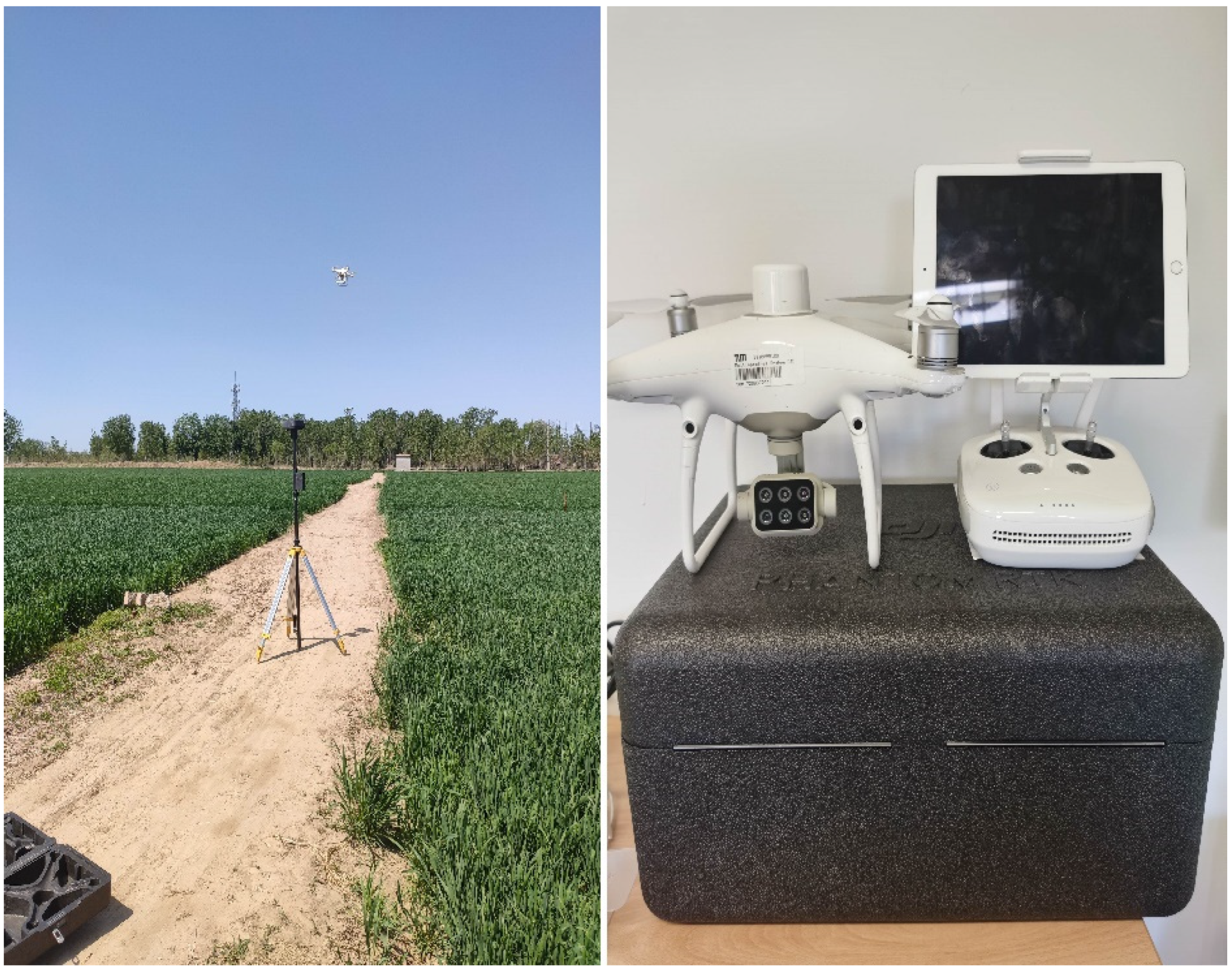
2.1. Study Area and Experimental Design

The experiment was conducted from 2020 to 2021 at the Wuqiao Experimental Station of China Agricultural University, which is located in Wuqiao County (37°41′ N, 116°37′ E), Hebei Province, China (Figure 1). The site is in the North China Plain and has a warm temperate semi-humid continental monsoon climate, average rainfall of 550 mm, an average temperature of 12.5 °C, and an average altitude of 18 m. The soil texture was determined to be light loam, which contains 11.9% clay, 78.1% silt, and 10.0% sand.
This experiment followed a split zone test design. We selected JiMai22 variety of winter wheat (Triticum aestivum L.) in this study, which has the largest plant area in China, and was sowed in October 2020 and harvested in June 2021 with a row spacing of 15 cm and a density of 430 × 104 ha−1. Five nitrogen fertilizer treatments were established, including 0 kg N ha−1 (N0), 80 kg N ha−1 (N1), 120 kg N ha−1 (N2), 160 kg N ha−1 (N3), and 200 kg N ha−1 (N4). For each treatment, three replications were conducted, and each plot area was 40 m2 (10 m × 4 m). For all treatments, we applied 120 kg P2O5 ha−1 and 90 kg K2O ha−1 to the soil as basal dressings, and the rest of the field managements are the same.

2.2. Data Acquisition and Processing

2.2.1. Field Data Acquisition

When the wheat grows to the observed growth period (see Table 1), a 20 cm plus 30 cm area of wheat was randomly selected in each plot. After sampling, the samples were placed in plastic bags and taken back to the laboratory immediately. The stems and leaves of wheat were separated and dried at 105 °C for 2 h and then at 75 °C until the samples maintained a constant weight [52]. We used a balance with an accuracy of 0.01 g to obtain the dry weight of the above-ground biomass of wheat.

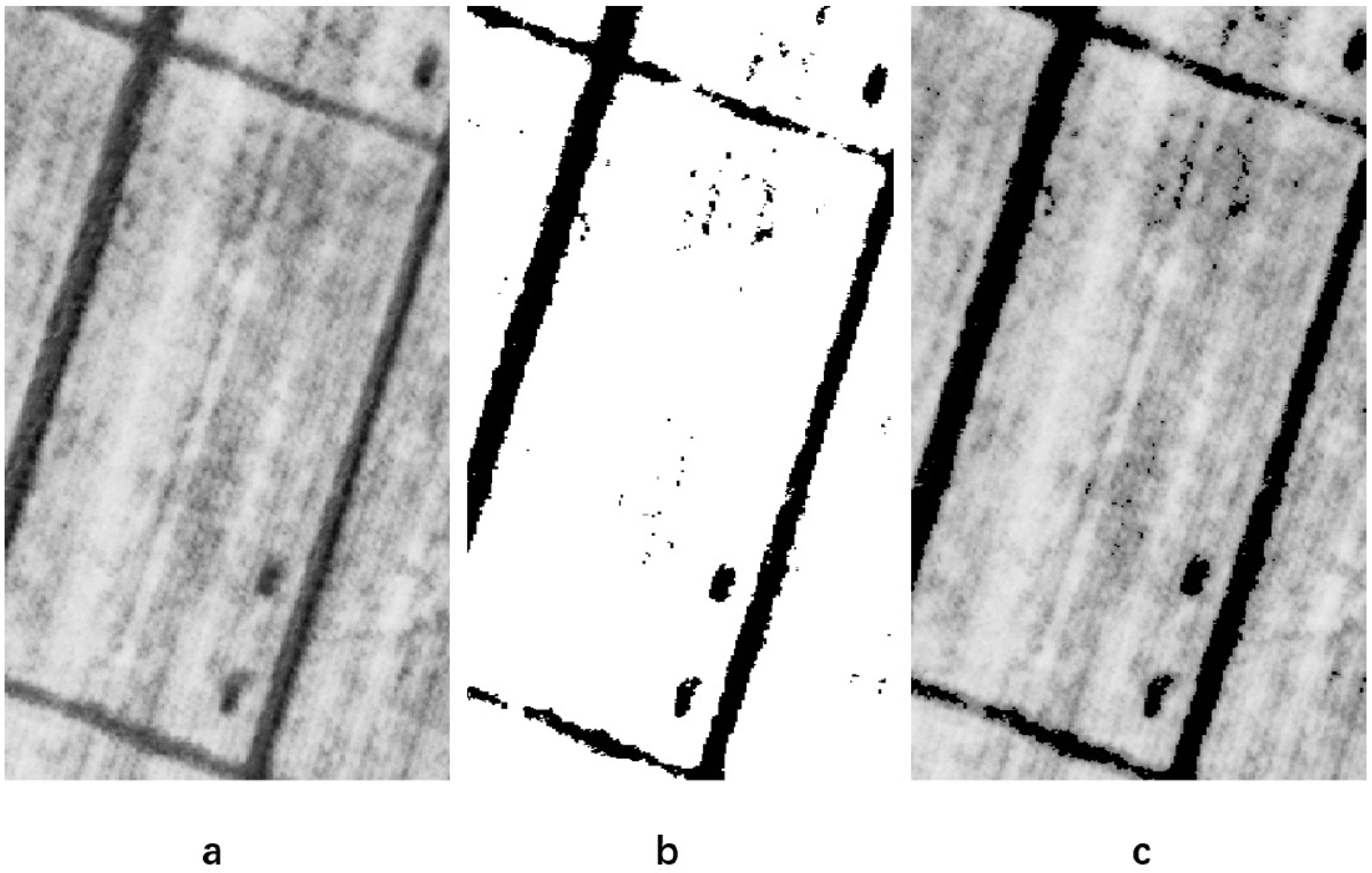
2.2.2. Acquisition and Pre-Processing of UAV Remote Sensing Data

During the wheat season, eight UAV flight missions were carried out between 10:00 a.m. to 14:00 p.m. on sunny days. Meanwhile, the dates of execution of the mission were the same as the dates of ground sampling. The UAV platform we used was a DJI Phantom 4 quadcopter (DJI, Shenzhen, Guangdong, China), which was equipped with a GPS/GNSS satellite positioning system, and with a maximum load capacity of 1.388 kg and a maximum flight time of 27 min. The sensor had six 1/2.9-inch CMOS, including one RGB sensor for visible light imaging and five monochromatic sensors including blue (450 nm ± 16 nm), green (560 nm ± 16 nm), red (650 nm ± 16 nm), red edge (730 nm ± 16 nm), and NIR (840 nm ± 26 nm) for multi-spectral imaging. For every single sensor, there were 2.08 million effective pixels (more details in Table 2). The fight route was made by DJI go pro software (DJI, Shenzhen, Guangdong, China), which provides easy mission planning through different methods such as setting points using the aircraft and importing files. The images were acquired with 80% overlap and 70% side overlap at the height of 25 m. Nine ground control points (GCP) were evenly placed on the field after the wheat emerged. We used a D-RTK 2 high-precision GNSS mobile station (DJI, Shenzhen, Guangdong, China) which has a centimeter-level positioning system with uninterrupted data transmission to record the coordinate information of GCPs. Figure 2 shows the scene of the drone working in the field.
Pix4D software (Pix4D SA, Lausanne, Switzerland), which integrates structure-from-motion (SFM) technology, was used to generate orthomosaic images. The SFM technology can search for the keypoints among the UAV-captured images. Camera parameters can be calibrated to external parameters, such as the position and scale of the images. At the same time, a point correlation was performed based on the characteristics to identify similar characteristics between images in common areas or overlapping areas. After computing the 3D position of matched points, the corresponding images were densified and textured. Then, by projecting each textured pixel onto a 2D plane, the orthomosaic image was obtained. We selected the multi-spectral Ag template as our model and manually punctured points by importing the coordinates of GCPs for orthomosaic georeferencing. Finally, five single-band orthophotos were obtained in each observed stage.

2.3. Methods

2.3.1. Selection of VIs

Forty-four VIs were selected to estimate above-ground biomass of winter wheat (see Table 3). All of the VIs were calculated from the original multi-spectral images.
Band math was performed in the QGIS 3.14 open-source software (QGIS Version 3.14). The orthophotos obtained from Pix4D software were imported into the new project of QGIS. We used the function of the raster calculator to perform the band math and generate the original vegetation index maps. In order to reduce the impact of abnormal factors such as soil, we applied image segmentation based on the OTSU algorithm in MATLAB (MathWorks, Natick, MA, USA) (Figure 3). Finally, QGIS software was used to extract the vegetation index of the region of interest.

2.3.2. Modeling Methods

For each growth stage, there were 15 remote sensing data points from regions of interest corresponding to the above-ground biomass data obtained by destructive sampling. In total, there were 120 samples across all stages. Linear regression (LR), partial least squares regression (PLSR), and random forests algorithm (RF) were used in this research. In individual growth stages, linear models based on each vegetation index were established for exploring the relationship between vegetation index and AGB. Meanwhile, models were built by PLSR and RF based on a pre-flowering dataset, post-flowering dataset, and a full dataset for determining the optimal combination of multi-spectral VIs and regression algorithms for predicting AGB of winter wheat in multiple growth stages. All the models were built in R programming language in R Studio (R Version 3.6.1) [83], using the R packages ‘pls’ [84] and ‘randomForest’ [85]. For the validation of models, 80% of the samples were selected as a training dataset, and the remaining 20% were used as a validation dataset.
PLSR is a bilinear regression method [86]. It integrates the advantages of principal component analysis, canonical correlation analysis, and linear regression analysis. It is stable, and suitable for small datasets and can handle multi-collinearity. The objective of partial least squares is to predict dependent variables from independent variables by describing the common structure of these two variables. PLSR can be used to identify potential factors, which are linear combinations of explanatory variables (also called latent variables) that best model the response variable. By performing component projection, it reduces noise and the dimensionality and eliminates the multi-collinearity of the input data. In this study, the one-sigma algorithm [87] was conducted to determine the optimal number of principal components. The variable importance in projection (VIP) [88] score is often used to assess the importance of variables, and the variables with a VIP score greater than one is generally considered to be more important. Therefore, we used it to evaluate the importance of the VIs in the PLSR model.
Random forest is an bagging-based ensemble algorithm [89]. By combining multiple weak classifiers, the final result is voted or averaged, so that the result of the overall model has higher accuracy and generalization performance. The generation rules of random forest are as follows: first, take N samples randomly from the dataset by the bootstrap way; second, use these data as the training set to train tree models; third, randomly select m feature subsets from M features, and select the best from these m features after each time the tree splits; fourth, the generated decision trees are formed into a random forest to ensure that each tree grows to the maximum extent, and there is no pruning process; finally, the mean value of the tree prediction results is used as the final prediction result. Furthermore, there are two important parameters to RF, which are the number of decision trees (ntree) and input variables per node (mtry). They are the key parameters to ensure the accuracy and complexity of the model. In this paper, to obtain the best RF model, the ntree and mtry were selected based on the RMSE with the RF algorithm. To further optimize the model, the 10-fold cross-validation was conducted and was repeated 5 times. In this study, %var explained by [89] was used for evaluating the performance of RF models. Percentage increase in mean squared error (%IncMSE) [40,90] was used as an indicator for evaluating the importance of variables in RF models. It comes from permuting out-of-bag (OOB) data, and the important variables have the higher %IncMSE after the data have been permutated. The detailed description of %IncMSE can be found in [89]. We used %IncMSE to evaluate the performance of VIs in RF model.

2.3.3. Evaluation of Model Accuracy

We choose the coefficients of determination (R2), root mean square error (RMSE), mean absolute error (MAE), and residual predictive deviation (RPD) to evaluate the performances of the different models. Generally, the higher the R2 and the lower the RMSE and MAE, the better the precision and accuracy of the models. The model is regarded as robust if the RPD is higher than 2 [91]. Equations (1)–(4) were used to calculate R2, RMSE, MAE, and PRD.
R 2 = i = 1 n ( x i x ¯ ) 2 ( y i y ¯ ) 2 / i = 1 n ( x i x ¯ ) 2 i = 1 n ( y i y ¯ ) 2
R M S E = 1 / k i = 1 n ( x i y i ) 2
M A E = i = 1 n | x i y i | / k
R P D =   S D y i / R M S E
where n is the number of samples, i is the ith sample, x i and y i stand for the estimated values and measured values, S D y i stands for the standard deviation of measured values, and x ¯ and y ¯ stand for the average estimated values and measured values, respectively. In order to understand the experiment more intuitively, the experiment flowchart (Figure 4) was made based on the experiment design, data collection, and processing.

3. Results

3.1. Variations of Winter Wheat Above-Ground Biomass

Table 4 shows the descriptive statistics of the above-ground biomass (AGB) by each growth stage. Across all stages, the AGB varies from 3.96 to 27.08 t/ha, with an SD of 5.51 and a CV of 36%. AGB showed an increasing trend as the growth stage progressed. It reached the maximum at the stage AF20 with a mean value of 20.44 t/ha.

3.2. AGB Model Based on LR

AGB was regressed on 44 VIs in each growth stage as well as the pre- and post-flowering period (BF and AF), and the results showed that most VIs have good capability to predict AGB in all observed stages with positive correlations, such as NDVI (Figure 5). Only a few VIs have a negative correlation with wheat AGB, such as SIPI (Supplementary Material S1). Decreased linear correlations between VIs and AGB for the BF (pre-flowering) period were found compared to the LR result at each individual pre-flowering stages, and there was little linear correlation between VIs and AGB throughout the AF (post-flowering) period. Moreover, we found a rapid decrease in NDVI at the stage AF5 (Figure 5b).
Comparing spectral indices between stages, the TCARI/OSAVI showed the best prediction of AGB, with an R2 of 0.93 at the heading stage. Figure 6 shows the top 10 VIs at each growth stage and the periods of BF and AF. From the jointing stage to AF25, the VIs with the best predictive capability were TCARI/OSAVI (R2 = 0.70), WDRVI (R2 = 0.86), TCARI/OSAVI (R2 = 0.93), GNDVI (R2 = 0.81), OSAVI-REG (R2 = 0.88), SIPI (R2 = 0.83), GARI (R2 = 0.75), and NDVI (R2 = 0.72), respectively. For the BF and AF, the best VIs were CVI (R2 = 0.67) and TCARI/OSAVI (R2 = 0.46). In general, as the growth progressed, the prediction capability of the VIs increased and reached the maximum at the heading stage, then gradually decreased.

3.3. AGB Model Based on PLSR

Three PLSR models were constructed based on the pre-flowering dataset, post-flowering dataset, and the whole dataset, respectively. Figure 7a–c shows the top VIs (VIP > 1) of the three PLSR models. Based on the VIP analysis (Figure S1, Supplementary Material S2), the indices of significant contribution (VIP ≥ 1) were determined for the pre- and post-flowering models, and the across-stage models, respectively, with nine, ten, and fifteen indices across-stage.
The most important indices for the three PLSR models were DVI-RGE (VIP = 2.08), TCARI/OSAVI (VIP = 2.12), and S-CCCI (VIP = 1.72), respectively. Three indices (TCARI/OSAVI, SIPI, OSAVI) were the same in the pre- and post-flowering PLSR models. Six indices (DVI-REG, TCARI/OSAVI, TCARI, OSAVI, CVI, SAVI) were the same in the pre-flowering and across-stage PLSR models. Seven indices (TCARI/OSAVI, OSAVI, OSAVI-REG, OSAVI-GREEN, MTCI, RGBVI, S-CCCI) were the same in the post-flowering and across-stage PLSR models. It is worth noting that TCARI/OSAVI and OSAVI were important contributions for all the three PLSR models.
As shown in Figure 8, the pre-flowering PLSR model with three components performed the best in the training set (R2 = 0.92, RMSE = 0.95 t/ha, MAE = 0.75 t/ha, and RPD = 3.67). The across-stage PLSR model with two components performed the worst in the training set (R2 = 0.74, RMSE = 2.82 t/ha, MAE = 2.18 t/ha, and RPD = 2.00), but performed the best for the validation set (R2 = 0.75, RMSE = 2.57 t/ha, MAE = 2.05 t/ha, and RPD = 1.89). The post-flowering PLSR model performed the worst for the validation set, with the R2 of 0.50, the RMSE of 2.07 t/ha, the MAE of 1.69 t/ha, and RPD of 1.45. Comparing the performances of the three PLSR models in the training and the validation datasets, the pre-flowering PLSR model allowed for the best prediction of AGB.

3.4. AGB Model Based on RF

Based on our result, the ntree and mtry were set to 41 and 24 for the pre-flowering RF model, 300 and 19 for the post-flowering RF model, and 737 and 38 for the across-stage RF model (Figure S2 in Supplementary Material S2).
The top 20 VIs for the three RF models are shown by the order of the %IncMSE of VIs in Figure 7d–f. MCARI2 with a %IncMSE of 6.20, OSAVI with a %IncMSE of 12.47, and TCARI/OSAVI with a %IncMSE of 46.98 showed the largest contributions to the pre- and post-flowering RF models, and the across-stage RF model. By conducting 10-fold cross-validation (Figure S3 in Supplementary Material S2), the three RF models were further optimized by setting the mtry to eight, twelve, and twelve, respectively. Four indices of significant contributions (MCARI2, LCI, CVI, TCARI) were the same in the pre-flowering and post-flowering RF models. Five indices (MCARI2, LCI, CVI, TCARI, GRVI) were the same in the pre-flowering and across-stage RF models. Ten indices (OSAVI, TCARI/OSAVI, S-CCCI, CVI, MCARI2, MTCI, SAVI, OSAVI-REG, TCARI, LCI) were the same in the post-flowering and across-stage RF models. Overall, MCARI2, LCI, CVI, and TCARI were the same for all the three RF models.
As shown in Figure 9, the pre-flowering RF model performed well in predicting AGB (R2 = 0.96, RMSE = 0.58 t/ha, MAE = 0.46 t/ha, and RPD = 5.39 in training dataset and R2 = 0.93, RMSE = 0.93 t/ha, MAE = 0.72 t/ha, and RPD = 3.79 in validation dataset). The post-flowering RF model performed the worst in predicting AGB (R2 = 0.95, RMSE = 1.08 t/ha, MAE = 0.89 t/ha, and RPD = 3.95 in training dataset and R2 = 0.83, RMSE = 2.34 t/ha, MAE = 2.01 t/ha, and RPD = 1.36 in validation dataset). The across-stage RF model performed the best among the three RF models (R2 = 0.97, RMSE = 0.84 t/ha, MAE = 0.67 t/ha, and RPD = 6.35 in training dataset and R2 = 0.87, RMSE = 2.10 t/ha, MAE = 1.54 t/ha, and RPD = 2.85 in validation dataset).

4. Discussion

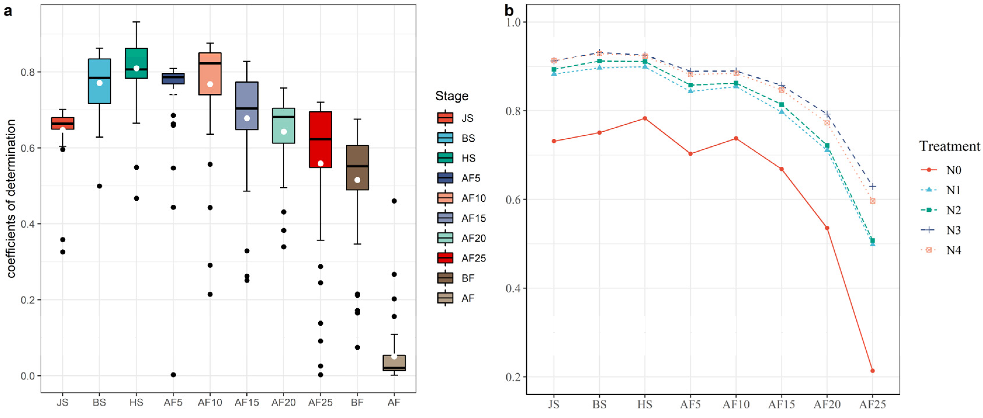
4.1. The Optimal Time Window for the AGB Monitoring

It can be found that the correlation between the VIs obtained from the UAV multi-spectral images and the AGB of winter wheat showed a trend of increasing first and then decreasing from the jointing stage to the stage AF25 in our study, except for the stage AF5 (Figure 6). After flowering, the correlation between VI and AGB becomes lower and lower. This may be due to the fact that photosynthesis is weakened [42] and the influence of wheat ears. The abrupt decrease in NDVI (Figure 5b) observed at the stage AF5 was deviated from the whole observation period, indicating that there might be some problems in the image acquisition at that time, in mid-May. There were many poplars planted around the farmland near the experimental site, and the stage AF5 was the time when the poplars spat out. There were many poplars in the air at that time, which floated on the wheat field and affected the quality of the images. Moreover, we found that with the advancement of the growth stages, the AGB has been increasing; but most of the VIs decreased and the degree of decrease gradually increased after flowering. This could explain the gradual decrease in the correlations between VIs and AGB after the heading stage.
Among all the stages, we found that the VIs at the heading stage had the best correlations with the AGB. It has also been found that the heading stage was suitable for monitoring the AGB of rice [29]. As a concurrent period between vegetative growth and reproductive growth of winter wheat, the heading stage is an important phenological stage for wheat [92]. Previous studies have demonstrated that the heading stage was the optimal crop growth stage for remote sensing of several agronomic traits such as grain yield and nitrogen uptake [93]. Furthermore, this can be explained from the perspective of radar remote sensing, such as in the study from Ouaadi [94], which showed that the C-band Sentinel-1 time-series data backscatter coefficient and polarization ratio of wheat reached the minimum and maximum at the heading stage, suggesting the heading stage is an optimal period for monitoring AGB.
It has been well known that vegetation indices often saturate in high-density vegetation canopies [95,96]. As the crop grows, canopy vegetation coverage gradually increases until it reaches the maximum or closure in the reproductive growth stage. In the later stages of crop growth, senescence may affect the use of multi-spectral data for crop biomass monitoring [29,97]. These could explain our results that the post-flowering biomass prediction models performed worse than the pre-flowering biomass prediction models. In crop management practices, pre-flowering biomass prediction is of practical value because most of the agronomic measures affecting crop growth are implemented during the vegetative growth period of crops.

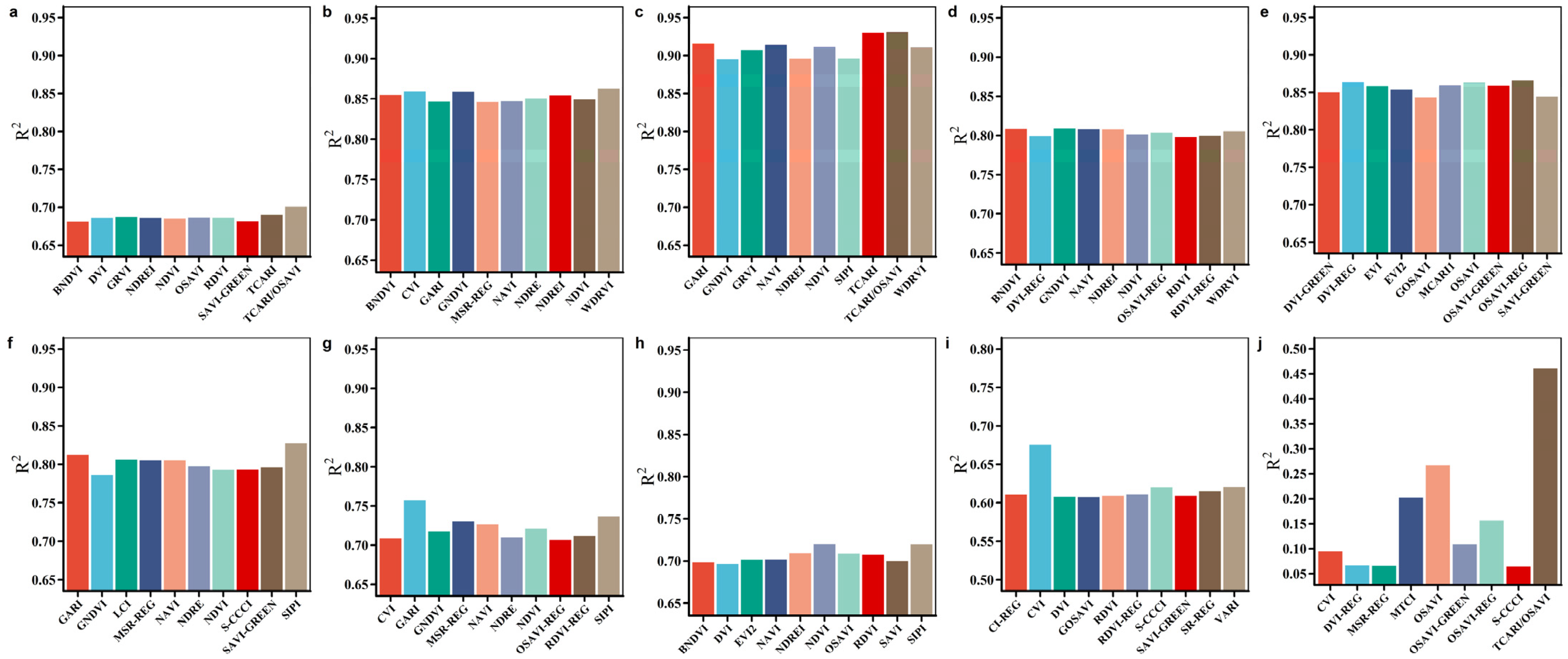
4.2. The Comparison of Sensitive Bands

In this study, we evaluated the relationship between each vegetation index and the AGB of winter wheat at each specific growth stage using the linear regression model. The Vis correlated highly with the AGB normally contained in the near-infrared and red bands for all the observation stages, although the best indices in each stage were not exactly the same. This is similar to the finding of a previous study [27], which proved the NIR region is the most effective band for AGB prediction in winter wheat. However, inconsistent results have also been reported that the VIs based on the NIR and red bands may fail to predict AGB in the middle and late stages of wheat growth [98].
According to the comparison of the best 10 VIs for different stages, we found that the best correlated VIs in the early stages were based on the red edge, green, and blue bands in addition to the NIR and red bands. In contrast, in the late stages, the best indices were found to be based exclusively on the NIR and red bands. Previous studies showed that plants have high reflectivity in the NIR band, and the light of the NIR band can penetrate deeper into the leaf and canopy than the visible bands [99,100]. Therefore, with the increase of crop biomass, the VIs based on visible bands may be less responsive to variations in biomass than the VIs based on the NIR bands.

4.3. The Performances of PLSR and RF Models for AGB Estimation

Preview studies have concluded that it was difficult to use traditional VIs to estimate crop multi-temporal variations in biomass due to the saturation of the VIs and their low sensitivity in the reproductive growth stages [42,101,102]. In this study, however, it was found to be feasible to predict the AGB of winter wheat across all stages by using multiple VIs and machine learning models. Since different VIs are calculated through different wavebands, the difference in their sensitivity to AGB may be significant in different growth stages. Meanwhile, compared to the use of VI-based linear models, the machine learning technique is suitable for tackling the multi-collinearity problem [103,104]. The RF models have achieved better estimation accuracy than the PLSR model in general, which is similar to previous studies [37,105]. Moreover, differently from the performance of the across-stage PLSR model, the across-stage RF model showed a better ability to predict wheat biomass than that of the pre-flowering RF model. Recent studies on predicting the AGB of various crops have shown the promise of using RF methods, such as in potato crops [21], wheat [106], rice [107], and corn [3,41]. Therefore, combining VIs and machine learning methods such as RF can help to overcome the saturation problem of using individual VIs in the late growth stage of winter wheat.
Among all the VIs used in this study, there were 28 two-band indices, 13 three-band indices, and 3 four-band indices. Our result showed that 24 of 44 VIs were selected by the machining learning models for estimating the AGB of winter wheat, including 13 two-band indices, 9 three-band indices, and 2 four-band indices. The three-band vegetation indices are expected to be less prone to the saturation problems than the two-band vegetation indices [58,108]. Actually, previous research has revealed the important role of the three-band vegetation index in crop monitoring due to its large amount of information and relatively simple structure [58,108]. Many studies on crop nitrogen monitoring used three-band or optimal three-band vegetation indices and obtained great results [109,110]. In this study, nearly all the three-band vegetation indices were selected by our machine learning models, and nearly half or more of the vegetation indices used in each model were three-band vegetation indices. This suggests that three-band indices deserve more attention in crop biomass forecasting.
LCI, CVI, and TCARI were screened for their importance in biomass estimation in both the pre-flowering PLSR model and pre-flowering RF model. These VIs have been reported in previous studies [7,111,112], suggesting that these VIs may be more stable to be used in PLSR and RF models for the forecast of winter wheat biomass before flowering. Our result showed that five important VIs including the TCARI/OSAVI, OSAVI, OSAVI-REG, MTCI, and SAVI-GREEN were always used in the post-flowering machine learning models. Interestingly, most of these indices were related to soil-line vegetation indices, which were developed to minimize soil background influence [113]. Similarly, TCARI/OSAVI also contributed a lot to AGB forecasting in both across-stage machine learning models. Zheng [29] also found that OSAVI exhibited the best relationship with AGB for the whole season and post-heading stages. Meanwhile, it was found that ten important VIs were always selected both in the across-stage PLSR and RF across-stage models. Nevertheless, these indices should be further evaluated in future research, such as whether they should be prioritized to be used in machine learning models for AGB prediction.

4.4. The Limitations of the Study and Suggestions for Future AGB Estimation

This study was conducted in an experimental field condition and only had a small sample size of 120, spanning eight growth stages. It has been demonstrated that the accuracy of biomass estimation highly depends on the prediction method and data type, and less on the sample size of its data [114]. Statistically, obtaining more samples in a larger region will improve the generalizability of the model. Based on the results of the LR models, we found that most of the VIs related to the AGB of winter wheat were based on the NIR and red bands. However, our results indicated that the performance of the VIs for the AGB prediction differs in growth stages due to the fact that the top VIs obtained in different stages were different. This confirms the influence of crop growth stages on the sensitivity and performance of VIs for estimating crop biophysical parameters [115,116,117,118]. Namely, it is challenging to determine a unique VI that is suitable for the prediction of the same crop biophysical parameters across different crop growth stages. It has been recommended to use multiple VIs to best capture agricultural crop characteristics due to the variety of VIs at different growth stages [116]. Similarly, in this study, using multiple VIs in PLSR and RF models might be adequate to capture the variations in biomass in different stages. Therefore, determining an optimal combination of VIs is promising to predict the AGB of crops across stages. In future work, we will further investigate the combination of vegetation indices to obtain a generic prediction model for AGB monitoring using multi-spectral UAVs and more ground samples over a larger area.

5. Conclusions

In this study, the multi-temporal measured AGB of winter wheat obtained by field sampling was associated with the corresponding images obtained by a consumer-grade drone carrying five-band sensors. Linear regression models were built based on individual VIs from each specific growth stage to select the best predicting stage for the AGB of winter wheat. PLSR and RF models based on the pre-flowering dataset, post-flowering dataset, and a full dataset were constructed to assess the feasibility of using multiple VIs to estimate the AGB of winter wheat during multiple growth stages and to explore the optimal period for biomass forecasting of winter wheat. Firstly, results indicate that the NIR and the red bands are important bands for winter wheat AGB monitoring. Secondly, the optimal time window for using individual vegetation indices to predict winter wheat AGB is before wheat flowering. Lastly, compared with the instability of wheat AGB monitoring for different growth stages based on linear regression, this study demonstrates that it is feasible to use multi-VI-based PLSR and RF models to estimate AGB for multiple growth stages, including both the vegetative growth and reproductive growth stages of winter wheat. Our further work will further explore the optimal combination of vegetation indices to obtain a generic prediction model for AGB monitoring using multi-spectral UAVs and more ground samples over a larger area.

Supplementary Materials

The following supporting information can be downloaded at: https://www.mdpi.com/article/10.3390/rs14051251/s1, Supplementary Material S1: LR results for different stages. Supplementary Material S2: Figures S1–S3.

Author Contributions

Experiments were designed by M.Y., F.W. and K.Y.; F.W., L.M., T.Z. and W.Q. performed the flight missions and completed the acquisition of above-ground biomass in the field; F.W. compiled the data and conducted the data analysis; W.L. provided software technical support. Z.W., Y.Z., Z.S. and K.Y. supervised the experiments; F.W. wrote the initial draft of the manuscript and F.L. and K.Y. revised and edited the manuscript. All authors have read and agreed to the published version of the manuscript.

Funding

This work was financially supported by the Key Research Projects of Hebei Province (grant number: 21327003D) and the China Agricultural Research System (CARS301).

Institutional Review Board Statement

Not applicable.

Informed Consent Statement

Not applicable.

Data Availability Statement

Not applicable.

Acknowledgments

We thank the Wuqiao Experimental Station of China Agricultural University for the experiment site and equipment. We are also grateful for Ying Liu, Chenhang Du, and Chunsheng Yao for their support in field sampling.

Conflicts of Interest

The authors declare no conflict of interest.

References

  1. Li, J.; Zhang, Z.; Liu, Y.; Yao, C.; Song, W.; Xu, X.; Zhang, M.; Zhou, X.; Gao, Y.; Wang, Z.; et al. Effects of micro-sprinkling with different irrigation amount on grain yield and water use efficiency of winter wheat in the North China Plain. Agric. Water Manag. 2019, 224, 105736. [Google Scholar] [CrossRef]
  2. Huang, J.; Sedano, F.; Huang, Y.; Ma, H.; Li, X.; Liang, S.; Tian, L.; Zhang, X.; Fan, J.; Wu, W. Assimilating a synthetic Kalman filter leaf area index series into the WOFOST model to improve regional winter wheat yield estimation. Agric. For. Meteorol. 2016, 216, 188–202. [Google Scholar] [CrossRef]
  3. Zhu, W.; Sun, Z.; Peng, J.; Huang, Y.; Li, J.; Zhang, J.; Yang, B.; Liao, X. Estimating Maize Above-Ground Biomass Using 3D Point Clouds of Multi-Source Unmanned Aerial Vehicle Data at Multi-Spatial Scales. Remote Sens. 2019, 11, 2678. [Google Scholar] [CrossRef] [Green Version]
  4. Han, L.; Yang, G.; Dai, H.; Xu, B.; Yang, H.; Feng, H.; Li, Z.; Yang, X. Modeling maize above-ground biomass based on machine learning approaches using UAV remote-sensing data. Plant Methods 2019, 15, 1–19. [Google Scholar] [CrossRef] [PubMed] [Green Version]
  5. Gil-Docampo, M.L.; Arza-García, M.; Ortiz-Sanz, J.; Martínez-Rodríguez, S.; Marcos-Robles, J.L.; Sánchez-Sastre, L.F. Above-ground biomass estimation of arable crops using UAV-based SfM photogrammetry. Geocarto Int. 2019, 35, 687–699. [Google Scholar] [CrossRef]
  6. He, L.; Wang, R.; Mostovoy, G.; Liu, J.; Chen, J.; Shang, J.; Liu, J.; McNairn, H.; Powers, J. Crop Biomass Mapping Based on Ecosystem Modeling at Regional Scale Using High Resolution Sentinel-2 Data. Remote Sens. 2021, 13, 806. [Google Scholar] [CrossRef]
  7. Yue, J.; Yang, G.; Tian, Q.; Feng, H.; Xu, K.; Zhou, C. Estimate of winter-wheat above-ground biomass based on UAV ultrahigh-ground-resolution image textures and vegetation indices. ISPRS J. Photogramm. Remote Sens. 2019, 150, 226–244. [Google Scholar] [CrossRef]
  8. Meng, S.; Pang, Y.; Zhang, Z.; Jia, W.; Li, Z. Mapping Aboveground Biomass using Texture Indices from Aerial Photos in a Temperate Forest of Northeastern China. Remote Sens. 2016, 8, 230. [Google Scholar] [CrossRef] [Green Version]
  9. Feng, D.; Xu, W.; He, Z.; Zhao, W.; Yang, M. Advances in plant nutrition diagnosis based on remote sensing and computer application. Neural Comput. Appl. 2020, 32, 16833–16842. [Google Scholar] [CrossRef]
  10. Curran, P.J.; Dungan, J.L.; Peterson, D.L. Estimating the foliar biochemical concentration of leaves with reflectance spectrometry: Testing the Kokaly and Clark methodologies. Remote Sens. Environ. 2001, 76, 349–359. [Google Scholar] [CrossRef]
  11. Mauser, W.; Bach, H.; Hank, T.; Zabel, F.; Putzenlechner, B. How spectroscopy from space will support world agriculture. In Proceedings of the 2012 IEEE International Geoscience and Remote Sensing Symposium, Munich, Germany, 12 November 2012; pp. 7321–7324. [Google Scholar] [CrossRef]
  12. Wang, L.J.; Zhang, G.M.; Wang, Z.Y.; Liu, J.G.; Shang, J.L.; Liang, L. Bibliometric Analysis of Remote Sensing Research Trend in Crop Growth Monitoring: A Case Study in China. Remote Sens. 2019, 11, 809. [Google Scholar] [CrossRef] [Green Version]
  13. Zha, H.; Miao, Y.; Wang, T.; Li, Y.; Zhang, J.; Sun, W.; Feng, Z.; Kusnierek, K. Improving Unmanned Aerial Vehicle Remote Sensing-Based Rice Nitrogen Nutrition Index Prediction with Machine Learning. Remote Sens. 2020, 12, 215. [Google Scholar] [CrossRef] [Green Version]
  14. Pinto, J.; Powell, S.; Peterson, R.; Rosalen, D.; Fernandes, O. Detection of Defoliation Injury in Peanut with Hyperspectral Proximal Remote Sensing. Remote Sens. 2020, 12, 3828. [Google Scholar] [CrossRef]
  15. Maimaitiyiming, M.; Sagan, V.; Sidike, P.; Kwasniewski, M.T. Dual Activation Function-Based Extreme Learning Machine (ELM) for Estimating Grapevine Berry Yield and Quality. Remote Sens. 2019, 11, 740. [Google Scholar] [CrossRef] [Green Version]
  16. Chen, P. Estimation of Winter Wheat Grain Protein Content Based on Multisource Data Assimilation. Remote Sens. 2020, 12, 3201. [Google Scholar] [CrossRef]
  17. Bispo, P.C.; Rodríguez-Veiga, P.; Zimbres, B.; De Miranda, S.D.C.; Cezare, C.H.G.; Fleming, S.; Baldacchino, F.; Louis, V.; Rains, D.; Garcia, M.; et al. Woody Aboveground Biomass Mapping of the Brazilian Savanna with a Multi-Sensor and Machine Learning Approach. Remote Sens. 2020, 12, 2685. [Google Scholar] [CrossRef]
  18. Hu, T.; Zhang, Y.; Su, Y.; Zheng, Y.; Lin, G.; Guo, Q. Mapping the Global Mangrove Forest Aboveground Biomass Using Multisource Remote Sensing Data. Remote Sens. 2020, 12, 1690. [Google Scholar] [CrossRef]
  19. Naik, P.; Dalponte, M.; Bruzzone, L. Prediction of Forest Aboveground Biomass Using Multitemporal Multispectral Remote Sensing Data. Remote Sens. 2021, 13, 1282. [Google Scholar] [CrossRef]
  20. Atzberger, C.; Darvishzadeh, R.; Immitzer, M.; Schlerf, M.; Skidmore, A.; le Maire, G. Comparative analysis of different retrieval methods for mapping grassland leaf area index using airborne imaging spectroscopy. Int. J. Appl. Earth Obs. Geoinf. 2015, 43, 19–31. [Google Scholar] [CrossRef] [Green Version]
  21. Yang, H.; Li, F.; Wang, W.; Yu, K. Estimating Above-Ground Biomass of Potato Using Random Forest and Optimized Hyperspectral Indices. Remote Sens. 2021, 13, 2339. [Google Scholar] [CrossRef]
  22. Féret, J.-B.; le Maire, G.; Jay, S.; Berveiller, D.; Bendoula, R.; Hmimina, G.; Cheraiet, A.; Oliveira, J.; Ponzoni, F.; Solanki, T.; et al. Estimating leaf mass per area and equivalent water thickness based on leaf optical properties: Potential and limitations of physical modeling and machine learning. Remote Sens. Environ. 2019, 231, 110959. [Google Scholar] [CrossRef]
  23. Feret, J.-B.; François, C.; Asner, G.P.; Gitelson, A.A.; Martin, R.E.; Bidel, L.P.; Ustin, S.L.; Le Maire, G.; Jacquemoud, S. PROSPECT-4 and 5: Advances in the leaf optical properties model separating photosynthetic pigments. Remote Sens. Environ. 2008, 112, 3030–3043. [Google Scholar] [CrossRef]
  24. Wang, Z.; Skidmore, A.K.; Darvishzadeh, R.; Heiden, U.; Heurich, M.; Wang, T. Leaf Nitrogen Content Indirectly Estimated by Leaf Traits Derived From the PROSPECT Model. IEEE J. Sel. Top. Appl. Earth Obs. Remote Sens. 2015, 8, 3172–3182. [Google Scholar] [CrossRef]
  25. Soenen, S.A.; Peddle, D.R.; Hall, R.J.; Coburn, C.A.; Hall, F.G. Estimating aboveground forest biomass from canopy reflectance model inversion in mountainous terrain. Remote Sens. Environ. 2010, 114, 1325–1337. [Google Scholar] [CrossRef]
  26. Wang, X.Y.; Guo, Y.G.; He, J. Estimation of forest biomass by integrating ALOS PALSAR And HJ1B data. Land Surf. Remote Sens. II 2014, 9260, 92603I. [Google Scholar] [CrossRef]
  27. Fu, Y.; Yang, G.; Wang, J.; Song, X.; Feng, H. Winter wheat biomass estimation based on spectral indices, band depth analysis and partial least squares regression using hyperspectral measurements. Comput. Electron. Agric. 2014, 100, 51–59. [Google Scholar] [CrossRef]
  28. Ferwerda, J.G.; Skidmore, A. Can nutrient status of four woody plant species be predicted using field spectrometry? ISPRS J. Photogramm. Remote Sens. 2007, 62, 406–414. [Google Scholar] [CrossRef]
  29. Zheng, H.; Cheng, T.; Zhou, M.; Li, D.; Yao, X.; Tian, Y.; Cao, W.; Zhu, Y. Improved estimation of rice aboveground biomass combining textural and spectral analysis of UAV imagery. Precis. Agric. 2019, 20, 611–629. [Google Scholar] [CrossRef]
  30. Zhang, L.; Verma, B.; Stockwell, D.; Chowdhury, S. Density Weighted Connectivity of Grass Pixels in image frames for biomass estimation. Expert Syst. Appl. 2018, 101, 213–227. [Google Scholar] [CrossRef] [Green Version]
  31. Tucker, C.J. Red and photographic infrared linear combinations for monitoring vegetation. Remote Sens. Environ. 1979, 8, 127–150. [Google Scholar] [CrossRef] [Green Version]
  32. Gnyp, M.L.; Miao, Y.; Yuan, F.; Ustin, S.L.; Yu, K.; Yao, Y.; Huang, S.; Bareth, G. Hyperspectral canopy sensing of paddy rice aboveground biomass at different growth stages. Field Crops Res. 2014, 155, 42–55. [Google Scholar] [CrossRef]
  33. Breunig, F.M.; Galvão, L.S.; Dalagnol, R.; Dauve, C.E.; Parraga, A.; Santi, A.L.; Della Flora, D.P.; Chen, S. Delineation of management zones in agricultural fields using cover–crop biomass estimates from PlanetScope data. Int. J. Appl. Earth Obs. Geoinf. 2020, 85, 102004. [Google Scholar] [CrossRef]
  34. Venancio, L.P.; Mantovani, E.C.; Amaral, C.H.D.; Neale, C.M.U.; Gonçalves, I.Z.; Filgueiras, R.; Eugenio, F.C. Potential of using spectral vegetation indices for corn green biomass estimation based on their relationship with the photosynthetic vegetation sub-pixel fraction. Agric. Water Manag. 2020, 236, 106155. [Google Scholar] [CrossRef]
  35. Pölönen, I.; Saari, H.; Kaivosoja, J.; Honkavaara, E.; Pesonen, L. Hyperspectral imaging based biomass and nitrogen content estimations from light-weight UAV. In Remote Sensing for Agriculture, Ecosystems, and Hydrology XV; SPIE: Bellingham, WA, USA, 2013; Volume 8887, pp. 141–149. [Google Scholar] [CrossRef]
  36. Kross, A.; McNairn, H.; Lapen, D.; Sunohara, M.; Champagne, C. Assessment of RapidEye vegetation indices for estimation of leaf area index and biomass in corn and soybean crops. Int. J. Appl. Earth Obs. Geoinf. 2015, 34, 235–248. [Google Scholar] [CrossRef] [Green Version]
  37. Liu, Y.; Liu, S.; Li, J.; Guo, X.; Wang, S.; Lu, J. Estimating biomass of winter oilseed rape using vegetation indices and texture metrics derived from UAV multispectral images. Comput. Electron. Agric. 2019, 166, 105026. [Google Scholar] [CrossRef]
  38. Li, S.; Potter, C. Patterns of Aboveground Biomass Regeneration in Post-Fire Coastal Scrub Communities. GIScience Remote Sens. 2012, 49, 182–201. [Google Scholar] [CrossRef]
  39. Deery, D.M.; Rebetzke, G.J.; Jimenez-Berni, J.A.; Condon, A.G.; Smith, D.J.; Bechaz, K.M.; Bovill, W.D. Ground-Based LiDAR Improves Phenotypic Repeatability of Above-Ground Biomass and Crop Growth Rate in Wheat. Plant Phenomics 2020, 2020, 1–11. [Google Scholar] [CrossRef]
  40. Varela, S.; Pederson, T.; Bernacchi, C.J.; Leakey, A.D.B. Understanding Growth Dynamics and Yield Prediction of Sorghum Using High Temporal Resolution UAV Imagery Time Series and Machine Learning. Remote Sens. 2021, 13, 1763. [Google Scholar] [CrossRef]
  41. Zhang, Y.; Xia, C.; Zhang, X.; Cheng, X.; Feng, G.; Wang, Y.; Gao, Q. Estimating the maize biomass by crop height and narrowband vegetation indices derived from UAV-based hyperspectral images. Ecol. Indic. 2021, 129, 107985. [Google Scholar] [CrossRef]
  42. Yue, J.; Feng, H.; Jin, X.; Yuan, H.; Li, Z.; Zhou, C.; Yang, G.; Tian, Q. A Comparison of Crop Parameters Estimation Using Images from UAV-Mounted Snapshot Hyperspectral Sensor and High-Definition Digital Camera. Remote Sens. 2018, 10, 1138. [Google Scholar] [CrossRef] [Green Version]
  43. Wang, Y.; Zhang, K.; Tang, C.; Cao, Q.; Tian, Y.; Zhu, Y.; Cao, W.; Liu, X. Estimation of Rice Growth Parameters Based on Linear Mixed-Effect Model Using Multispectral Images from Fixed-Wing Unmanned Aerial Vehicles. Remote Sens. 2019, 11, 1371. [Google Scholar] [CrossRef] [Green Version]
  44. Yue, J.; Feng, H.; Yang, G.; Li, Z. A Comparison of Regression Techniques for Estimation of Above-Ground Winter Wheat Biomass Using Near-Surface Spectroscopy. Remote Sens. 2018, 10, 66. [Google Scholar] [CrossRef] [Green Version]
  45. Zhang, J.; Tian, H.; Wang, D.; Li, H.; Mouazen, A.M. A Novel Approach for Estimation of Above-Ground Biomass of Sugar Beet Based on Wavelength Selection and Optimized Support Vector Machine. Remote Sens. 2020, 12, 620. [Google Scholar] [CrossRef] [Green Version]
  46. Dong, L.; Du, H.; Han, N.; Li, X.; Zhu, D.; Mao, F.; Zhang, M.; Zheng, J.; Liu, H.; Huang, Z.; et al. Application of Convolutional Neural Network on Lei Bamboo Above-Ground-Biomass (AGB) Estimation Using Worldview-2. Remote Sens. 2020, 12, 958. [Google Scholar] [CrossRef] [Green Version]
  47. Bhardwaj, A.; Sam, L.; Akanksha; Martín-Torres, F.J.; Kumar, R. UAVs as remote sensing platform in glaciology: Present applications and future prospects. Remote Sens. Environ. 2016, 175, 196–204. [Google Scholar] [CrossRef]
  48. Qiu, Z.; Ma, F.; Li, Z.; Xu, X.; Ge, H.; Du, C. Estimation of nitrogen nutrition index in rice from UAV RGB images coupled with machine learning algorithms. Comput. Electron. Agric. 2021, 189, 106421. [Google Scholar] [CrossRef]
  49. Zhang, X.; Han, L.; Dong, Y.; Shi, Y.; Huang, W.; Han, L.; González-Moreno, P.; Ma, H.; Ye, H.; Sobeih, T. A Deep Learning-Based Approach for Automated Yellow Rust Disease Detection from High-Resolution Hyperspectral UAV Images. Remote Sens. 2019, 11, 1554. [Google Scholar] [CrossRef] [Green Version]
  50. Han, X.; Wei, Z.; Chen, H.; Zhang, B.; Li, Y.; Du, T. Inversion of Winter Wheat Growth Parameters and Yield Under Different Water Treatments Based on UAV Multispectral Remote Sensing. Front. Plant Sci. 2021, 12, 1–13. [Google Scholar] [CrossRef]
  51. Roth, L.; Aasen, H.; Walter, A.; Liebisch, F. Extracting leaf area index using viewing geometry effects—A new perspective on high-resolution unmanned aerial system photography. ISPRS J. Photogramm. Remote Sens. 2018, 141, 161–175. [Google Scholar] [CrossRef]
  52. Jiang, Q.; Fang, S.; Peng, Y.; Gong, Y.; Zhu, R.; Wu, X.; Ma, Y.; Duan, B.; Liu, J. UAV-Based Biomass Estimation for Rice-Combining Spectral, TIN-Based Structural and Meteorological Features. Remote Sens. 2019, 11, 890. [Google Scholar] [CrossRef] [Green Version]
  53. Wang, F.-M.; Huang, J.-F.; Tang, Y.-L.; Wang, X.-Z. New Vegetation Index and Its Application in Estimating Leaf Area Index of Rice. Rice Sci. 2007, 14, 195–203. [Google Scholar] [CrossRef]
  54. Gitelson, A.A.; Gritz, Y.; Merzlyak, M.N. Relationships between leaf chlorophyll content and spectral reflectance and algorithms for non-destructive chlorophyll assessment in higher plant leaves. J. Plant Physiol. 2003, 160, 271–282. [Google Scholar] [CrossRef]
  55. Clevers, J.G.P.W.; Kooistra, L.; Brande, M.M.M.V.D. Using Sentinel-2 Data for Retrieving LAI and Leaf and Canopy Chlorophyll Content of a Potato Crop. Remote Sens. 2017, 9, 405. [Google Scholar] [CrossRef] [Green Version]
  56. Vincini, M.; Frazzi, E.; D’Alessio, P. A broad-band leaf chlorophyll vegetation index at the canopy scale. Precis. Agric. 2008, 9, 303–319. [Google Scholar] [CrossRef]
  57. Rouse, J.W.; Haas, R.H.; Schell, J.A.; Deeering, D. Monitoring Vegetation Systems in the Great Plains with ERTS (Earth Resources Technology Satellite). In Proceedings of the Third Earth Resources Technology Satellite-1 Symposium, Washington, DC, USA, 10–14 December 1973; Volume 1, pp. 309–317. Available online: https://ntrs.nasa.gov/citations/19740022614 (accessed on 26 January 2022).
  58. Huete, A.; Didan, K.; Miura, T.; Rodriguez, E.P.; Gao, X.; Ferreira, L.G. Overview of the radiometric and biophysical performance of the MODIS vegetation indices. Remote Sens. Environ. 2002, 83, 195–213. [Google Scholar] [CrossRef]
  59. Jiang, Z.; Huete, A.R.; Didan, K.; Miura, T. Development of a two-band enhanced vegetation index without a blue band. Remote Sens. Environ. 2008, 112, 3833–3845. [Google Scholar] [CrossRef]
  60. Gitelson, A.A.; Merzlyak, M.N.; Lichtenthaler, H.K. Detection of Red Edge Position and Chlorophyll Content by Reflectance Measurements Near 700 nm. J. Plant Physiol. 1996, 148, 501–508. [Google Scholar] [CrossRef]
  61. Siegmann, B.; Jarmer, T.; Lilienthal, H.; Richter, N.; Selige, T.; Höfled, B. Comparison of narrow band vegetation indices and empirical models from hyperspectral remote sensing data for the assessment of wheat nitrogen concentration. In Proceedings of the 8th EARSeL Workshop on Imaging Spectroscopy, Nantes, France, 1 January 2013; pp. 1–2. [Google Scholar]
  62. Xiao, Y.; Zhao, W.; Zhou, D.; Gong, H. Sensitivity Analysis of Vegetation Reflectance to Biochemical and Biophysical Variables at Leaf, Canopy, and Regional Scales. IEEE Trans. Geosci. Remote Sens. 2014, 52, 4014–4024. [Google Scholar] [CrossRef]
  63. Daughtry, C.S.T.; Walthall, C.L.; Kim, M.S.; De Colstoun, E.B.; McMurtrey, J.E. Estimating Corn Leaf Chlorophyll Concentration from Leaf and Canopy Reflectance. Remote. Sens. Environ. 2000, 74, 229–239. [Google Scholar] [CrossRef]
  64. Haboudane, D.; Miller, J.R.; Pattey, E.; Zarco-Tejada, P.J.; Strachan, I.B. Hyperspectral vegetation indices and novel algorithms for predicting green LAI of crop canopies: Modeling and validation in the context of precision agriculture. Remote Sens. Environ. 2004, 90, 337–352. [Google Scholar] [CrossRef]
  65. Gong, P.; Pu, R.; Biging, G.; Larrieu, M. Estimation of forest leaf area index using vegetation indices derived from hyperion hyperspectral data. IEEE Trans. Geosci. Remote Sens. 2003, 41, 1355–1362. [Google Scholar] [CrossRef] [Green Version]
  66. Chen, J.M. Evaluation of Vegetation Indices and a Modified Simple Ratio for Boreal Applications. Can. J. Remote Sens. 1996, 22, 229–242. [Google Scholar] [CrossRef]
  67. Dash, J.; Curran, P.J. The MERIS terrestrial chlorophyll index. Int. J. Remote Sens. 2004, 25, 5403–5413. [Google Scholar] [CrossRef]
  68. Gitelson, A.A.; Merzlyak, M.N. Remote estimation of chlorophyll content in higher plant leaves. Int. J. Remote 1997, 18, 2691–2697. [Google Scholar] [CrossRef]
  69. Hassan, M.A.; Yang, M.; Rasheed, A.; Jin, X.; Xia, X.; Xiao, Y.; He, Z. Time-Series Multispectral Indices from Unmanned Aerial Vehicle Imagery Reveal Senescence Rate in Bread Wheat. Remote Sens. 2018, 10, 809. [Google Scholar] [CrossRef] [Green Version]
  70. Agapiou, A.; Alexakis, D.D.; Stavrou, M.; Sarris, A.; Themistocleous, K.; Hadjimitsis, D.G. Prospects and limitations of vegetation indices in archeological research: The Neolithic Thessaly case study. SPIE Remote Sens. 2013, IV, 88930D. [Google Scholar] [CrossRef]
  71. Rondeaux, G.; Steven, M.; Baret, F. Optimization of soil-adjusted vegetation indices. Remote Sens. Environ. 1996, 55, 95–107. [Google Scholar] [CrossRef]
  72. Roujean, J.-L.; Breon, F.-M. Estimating PAR absorbed by vegetation from bidirectional reflectance measurements. Remote Sens. Environ. 1995, 51, 375–384. [Google Scholar] [CrossRef]
  73. Bendig, J.; Yu, K.; Aasen, H.; Bolten, A.; Bennertz, S.; Broscheit, J.; Gnyp, M.L.; Bareth, G. Combining UAV-based plant height from crop surface models, visible, and near infrared vegetation indices for biomass monitoring in barley. Int. J. Appl. Earth Obs. Geoinf. 2015, 39, 79–87. [Google Scholar] [CrossRef]
  74. Walsh, O.S.; Shafian, S.; Marshall, J.M.; Jackson, C.; McClintick-Chess, J.R.; Blanscet, S.M.; Swoboda, K.; Thompson, C.; Belmont, K.M.; Walsh, W.L. Assessment of UAV Based Vegetation Indices for Nitrogen Concentration Estimation in Spring Wheat. Adv. Remote Sens. 2018, 7, 71–90. [Google Scholar] [CrossRef] [Green Version]
  75. Huete, A.R. A soil-adjusted vegetation index (SAVI). Remote Sens. Environ. 1988, 25, 295–309. [Google Scholar] [CrossRef]
  76. Verrelst, J.; Schaepman, M.; Koetz, B.; Kneubühler, M. Angular sensitivity analysis of vegetation indices derived from CHRIS/PROBA data. Remote Sens. Environ. 2008, 112, 2341–2353. [Google Scholar] [CrossRef]
  77. Raper, T.B.; Varco, J.J. Canopy-scale wavelength and vegetative index sensitivities to cotton growth parameters and nitrogen status. Precis. Agric. 2014, 16, 62–76. [Google Scholar] [CrossRef] [Green Version]
  78. Penuelas, J.; Gamon, J.; Fredeen, A.; Merino, J.; Field, C. Reflectance indices associated with physiological changes in nitrogen- and water-limited sunflower leaves. Remote Sens. Environ. 1994, 48, 135–146. [Google Scholar] [CrossRef]
  79. Haboudane, D.; Miller, J.R.; Tremblay, N.; Zarco-Tejada, P.J.; Dextraze, L. Integrated narrow-band vegetation indices for prediction of crop chlorophyll content for application to precision agriculture. Remote Sens. Environ. 2002, 81, 416–426. [Google Scholar] [CrossRef]
  80. Broge, N.H.; Leblanc, E. Comparing prediction power and stability of broadband and hyperspectral vegetation indices for estimation of green leaf area index and canopy chlorophyll density. Remote Sens. Environ. 2001, 76, 156–172. [Google Scholar] [CrossRef]
  81. Gitelson, A.A.; Kaufman, Y.J.; Robert, S.; Rundquist, D. Novel algorithms for remote estimation of vegetation fraction. Remote Sens. Environ. 2002, 80, 76–87. [Google Scholar] [CrossRef] [Green Version]
  82. Gitelson, A.A. Remote estimation of crop fractional vegetation cover: The use of noise equivalent as an indicator of performance of vegetation indices. Int. J. Remote Sens. 2013, 34, 6054–6066. [Google Scholar] [CrossRef]
  83. Pilson, D.; Decker, K.L. Compensation for herbivory in wild sunflower: Response to simulated damage by the head-clipping weevil. Ecology 2002, 83, 3097–3107. [Google Scholar] [CrossRef]
  84. Mevik, B.-H.; Wehrens, R. TheplsPackage: Principal Component and Partial Least Squares Regression inR. J. Stat. Softw. 2007, 18, 1–23. [Google Scholar] [CrossRef] [Green Version]
  85. Liaw, A.; Wiener, M. Package ‘randomForest’. Breiman and Cutler’s Random Forests for Classification and Regression. Tutorial 2015, 29. Available online: https://cran.r-project.org/web/packages/randomForest/index.html (accessed on 26 January 2022).
  86. Pak, S.I.; Oh, T.H. Correlation and simple linear regression. J. Vet. Clin. 2010, 27, 427–434. [Google Scholar]
  87. Wold, S.; Sjostrom, M.; Eriksson, L. PLS-regression: A basic tool of chemometrics. Chemom. Intell. Lab. Syst. 2001, 58, 109–130. [Google Scholar] [CrossRef]
  88. Hastie, T.; Tibshirani, R.; Friedman, J. The Elements of Statistical Learning: Data Mining, Inference and Prediction. Math. Intell. 2005, 27, 83–85. [Google Scholar]
  89. Farrés, M.; Platikanov, S.; Tsakovski, S.; Tauler, R. Comparison of the variable importance in projection (VIP) and of the selectivity ratio (SR) methods for variable selection and interpretation. J. Chemom. 2015, 29, 528–536. [Google Scholar] [CrossRef]
  90. Breiman, L. Random forests. Mach. Learn. 2001, 45, 5–32. [Google Scholar] [CrossRef] [Green Version]
  91. Aiyelokun, O.O.; Agbede, O.A. Development of random forest model as decision support tool in water resources management of Ogun headwater catchments. Appl. Water Sci. 2021, 11, 1–9. [Google Scholar] [CrossRef]
  92. Huang, X.; Zhu, W.; Wang, X.; Zhan, P.; Liu, Q.; Li, X.; Sun, L. A Method for Monitoring and Forecasting the Heading and Flowering Dates of Winter Wheat Combining Satellite-Derived Green-Up Dates and Accumulated Temperature. Remote Sens. 2020, 12, 3536. [Google Scholar] [CrossRef]
  93. Pavuluri, K.; Chim, B.K.; Griffey, C.A.; Reiter, M.S.; Balota, M.; Thomason, W.E. Canopy spectral reflectance can predict grain nitrogen use efficiency in soft red winter wheat. Precis. Agric. 2014, 16, 405–424. [Google Scholar] [CrossRef]
  94. Ouaadi, N.; Jarlan, L.; Ezzahar, J.; Zribi, M.; Khabba, S.; Bouras, E.; Bousbih, S.; Frison, P.-L. Monitoring of wheat crops using the backscattering coefficient and the interferometric coherence derived from Sentinel-1 in semi-arid areas. Remote Sens. Environ. 2020, 251, 112050. [Google Scholar] [CrossRef]
  95. Sun, G.; Jiao, Z.; Zhang, A.; Li, F.; Fu, H.; Li, Z. Hyperspectral image-based vegetation index (HSVI): A new vegetation index for urban ecological research. Int. J. Appl. Earth Obs. Geoinf. 2021, 103, 102529. [Google Scholar] [CrossRef]
  96. Song, C. Optical remote sensing of forest leaf area index and biomass. Prog. Phys. Geogr. Earth Environ. 2013, 37, 98–113. [Google Scholar] [CrossRef]
  97. Guo, J.; Pradhan, S.; Shahi, D.; Khan, J.; McBreen, J.; Bai, G.; Murphy, J.P.; Babar, A. Increased Prediction Accuracy Using Combined Genomic Information and Physiological Traits in A Soft Wheat Panel Evaluated in Multi-Environments. Sci. Rep. 2020, 10, 1–12. [Google Scholar] [CrossRef]
  98. Yue, J.; Yang, G.; Li, C.; Li, Z.; Wang, Y.; Feng, H.; Xu, B. Estimation of Winter Wheat Above-Ground Biomass Using Unmanned Aerial Vehicle-Based Snapshot Hyperspectral Sensor and Crop Height Improved Models. Remote Sens. 2017, 9, 708. [Google Scholar] [CrossRef] [Green Version]
  99. Thenkabail, P.S.; Smith, R.B.; De Pauw, E. Hyperspectral Vegetation Indices and Their Relationships with Agricultural Crop Characteristics. Remote Sens. Environ. 2000, 71, 158–182. [Google Scholar] [CrossRef]
  100. Hatfield, J.L.; Gitelson, A.A.; Schepers, J.S.; Walthall, C.L. Application of Spectral Remote Sensing for Agronomic Decisions. Agron. J. 2008, 100, S-117–S-131. [Google Scholar] [CrossRef] [Green Version]
  101. Nguy-Robertson, A.; Gitelson, A.; Peng, Y.; Viña, A.; Arkebauer, T.; Rundquist, D. Green Leaf Area Index Estimation in Maize and Soybean: Combining Vegetation Indices to Achieve Maximal Sensitivity. Agron. J. 2012, 104, 1336–1347. [Google Scholar] [CrossRef] [Green Version]
  102. Luo, S.; He, Y.; Li, Q.; Jiao, W.; Zhu, Y.; Zhao, X. Nondestructive estimation of potato yield using relative variables derived from multi-period LAI and hyperspectral data based on weighted growth stage. Plant Methods 2020, 16, 1–14. [Google Scholar] [CrossRef]
  103. Martínez-Muñoz, G.; Suárez, A. Out-of-bag estimation of the optimal sample size in bagging. Pattern Recognit. 2010, 43, 143–152. [Google Scholar] [CrossRef] [Green Version]
  104. Garg, A.; Tai, K. Comparison of statistical and machine learning methods in modelling of data with multicollinearity. Int. J. Model. Identif. Control 2013, 18, 295. [Google Scholar] [CrossRef]
  105. Yue, J.; Yang, G.; Feng, H. Comparative of remote sensing estimation models of winter wheat biomass based on random forest algorithm. Nongye Gongcheng Xuebao/Transactions Chinese. Soc. Agric. Eng. 2016, 32, 175–182. [Google Scholar] [CrossRef]
  106. Lu, N.; Zhou, J.; Han, Z.; Li, D.; Cao, Q.; Yao, X.; Tian, Y.; Zhu, Y.; Cao, W.; Cheng, T. Improved estimation of aboveground biomass in wheat from RGB imagery and point cloud data acquired with a low-cost unmanned aerial vehicle system. Plant Methods 2019, 15, 17. [Google Scholar] [CrossRef] [PubMed] [Green Version]
  107. Cen, H.; Wan, L.; Zhu, J.; Li, Y.; Li, X.; Zhu, Y.; Weng, H.; Wu, W.; Yin, W.; Xu, C.; et al. Dynamic monitoring of biomass of rice under different nitrogen treatments using a lightweight UAV with dual image-frame snapshot cameras. Plant Methods 2019, 15, 32. [Google Scholar] [CrossRef]
  108. Sims, D.A.; Gamon, J.A. Relationships between leaf pigment content and spectral reflectance across a wide range of species, leaf structures and developmental stages. Remote Sens. Environ. 2002, 81, 337–354. [Google Scholar] [CrossRef]
  109. Li, F.; Mistele, B.; Hu, Y.; Chen, X.; Schmidhalter, U. Optimising three-band spectral indices to assess aerial N concentration, N uptake and aboveground biomass of winter wheat remotely in China and Germany. ISPRS J. Photogramm. Remote Sens. 2014, 92, 112–123. [Google Scholar] [CrossRef]
  110. Wang, W.; Yao, X.; Yao, X.; Tian, Y.; Liu, X.; Ni, J.; Cao, W.; Zhu, Y. Estimating leaf nitrogen concentration with three-band vegetation indices in rice and wheat. Field Crop. Res. 2012, 129, 90–98. [Google Scholar] [CrossRef]
  111. Badreldin, N.; Sanchez-Azofeifa, A. Estimating Forest Biomass Dynamics by Integrating Multi-Temporal Landsat Satellite Images with Ground and Airborne LiDAR Data in the Coal Valley Mine, Alberta, Canada. Remote Sens. 2015, 7, 2832–2849. [Google Scholar] [CrossRef] [Green Version]
  112. Foster, A.J.; Kakani, V.G.; Ge, J.; Mosali, J. Discrimination of Switchgrass Cultivars and Nitrogen Treatments Using Pigment Profiles and Hyperspectral Leaf Reflectance Data. Remote Sens. 2012, 4, 2576–2594. [Google Scholar] [CrossRef] [Green Version]
  113. Barillé, L.; Mouget, J.-L.; Méléder, V.; Rosa, P.; Jesus, B. Spectral response of benthic diatoms with different sediment backgrounds. Remote Sens. Environ. 2011, 115, 1034–1042. [Google Scholar] [CrossRef]
  114. Masjedi, A.; Zhao, J.; Thompson, A.M.; Yang, K.-W.; Flatt, J.E.; Crawford, M.M.; Ebert, D.S.; Tuinstra, M.R.; Hammer, G.; Chapman, S. Sorghum Biomass Prediction Using Uav-Based Remote Sensing Data and Crop Model Simulation. In Proceedings of the IGARSS 2018—2018 IEEE International Geoscience and Remote Sensing Symposium, Valencia, Spain, 22–27 July 2018; pp. 7719–7722. [Google Scholar]
  115. Yu, K.; Li, F.; Gnyp, M.L.; Miao, Y.; Bareth, G.; Chen, X. Remotely detecting canopy nitrogen concentration and uptake of paddy rice in the Northeast China Plain. ISPRS J. Photogramm. Remote Sens. 2013, 78, 102–115. [Google Scholar] [CrossRef]
  116. Hatfield, J.L.; Prueger, J.H. Value of Using Different Vegetative Indices to Quantify Agricultural Crop Characteristics at Different Growth Stages under Varying Management Practices. Remote Sens. 2010, 2, 562–578. [Google Scholar] [CrossRef] [Green Version]
  117. Li, F.; Miao, Y.; Hennig, S.D.; Gnyp, M.L.; Chen, X.; Jia, L.; Bareth, G. Evaluating hyperspectral vegetation indices for estimating nitrogen concentration of winter wheat at different growth stages. Precis. Agric. 2010, 11, 335–357. [Google Scholar] [CrossRef]
  118. Yu, K.; Lenz-Wiedemann, V.; Chen, X.; Bareth, G. Estimating leaf chlorophyll of barley at different growth stages using spectral indices to reduce soil background and canopy structure effects. ISPRS J. Photogramm. Remote Sens. 2014, 97, 58–77. [Google Scholar] [CrossRef]
Figure 1. Location of the study area and overview of the experiment site. The red words inside the black boxes represent different treatment.
Remotesensing 14 01251 g001
Figure 2. The UAV platform used in this study.
Remotesensing 14 01251 g002
Figure 3. (a) Original vegetation index image; (b) binary vegetation index image based on OTSU method; (c) segmented vegetation index image.
Remotesensing 14 01251 g003
Figure 4. The flowchart of the experiment.
Remotesensing 14 01251 g004
Figure 5. (a) Variations of the R2 of different VIs in different growth stages. The white dots in each box represent the mean value of R2, and the black dots represent outliers. (b) The NDVI of different treatments across all stages.
Remotesensing 14 01251 g005
Figure 6. Top 10 VIs for specific growth stages using LR. (a) JS, (b) BS, (c) HS, (d) AF5, (e) AF10, (f) AF15, (g) AF20, (h) AF25, (i) BF, (j) AF.
Remotesensing 14 01251 g006
Figure 7. The vegetation indices with VIP scores greater than one in the PLSR models and the top 20 VIs for RF models. (a) VIP for pre-flowering PLSR model; (b) VIP for post-flowering PLSR model; (c) VIP for across-stage PLSR model; (d) %IncMSE for pre-flowering RF model; (e) %IncMSE for post-flowering RF model; (f) %IncMSE for across-stage RF model.
Remotesensing 14 01251 g007
Figure 8. Comparison of the prediction of AGB using different PLSR models for the training and validation datasets. (a) The prediction of AGB using pre-flowering PLSR model for the training dataset; (b) the prediction of AGB using pre-flowering PLSR model for the validation dataset; (c) the prediction of AGB using post-flowering PLSR model for the training dataset; (d) the prediction of AGB using post-flowering PLSR model for the validation dataset; (e) the prediction of AGB using across-stage PLSR model for the training dataset; (f) the prediction of AGB using across-stage PLSR model for the validation dataset.
Remotesensing 14 01251 g008
Figure 9. The prediction effect of RF model using different datasets in the training and validation datasets: (a) the prediction of AGB using pre-flowering RF model for the training dataset; (b) the prediction of AGB using pre-flowering RF model for the validation dataset; (c) the prediction of AGB using post-flowering RF model for the training dataset; (d) the prediction of AGB using post-flowering RF model for the validation dataset; (e) the prediction of AGB using across-stage RF model for the training dataset; (f) the prediction of AGB using across-stage RF model for the validation dataset.
Remotesensing 14 01251 g009
Table 1. Sampling date and the growth stage of wheat.
Sampling DateGrowth StageZadoks Codes
18 April 2021Jointing stage (JS)GS31
27 April 2021 Booting stage (BS)GS40
5 May 2021Heading stage (HS)GS50
12 May 20215 Days after Flowering (AF5)GS70
17 May 202110 Days after Flowering (AF10)GS75
22 May 202115 Days after Flowering (AF15)GS80
27 May 202120 Days after Flowering (AF20)GS85
1 June 202125 Days after Flowering (AF25)GS90
Table 2. Some parameters of the UAV and sensor.
Aircraft Parameters Camera Parameters
Takeoff Weight1487 gFOV62.7°
Diagonal Distance 350 mmFocal Length5.74 mm
Maximum Flying Altitude6000 mAperturef/2.2
Max Ascent Speed6 m/sRGB Sensor ISO200–800
Max Descent Speed3 m/sMonochrome Sensor Gain1–8 ×
Max Speed50 km/hMax Image Size1600 × 1300
Max Flight Time27 minPhoto FormatJPEG/TIFF
Operating Temperature0 to 40 °CSupported File Systems≥32 GB
Operating Frequency5.72 to 5.85 GHzOperating Temperature0° to 40 °C
Table 3. Vegetation indices used in this study.
IndexFormulaAuthors
BNDVI ( N I R B L U E ) / ( N I R + B L U E ) [53]
CI-GREEN ( N I R / G R E E N ) 1 [54]
CI-RED ( N I R / R E D ) 1 [55]
CI-REG ( N I R / R E D E D G E ) 1 [54]
CVI ( N I R / G R E E N ) × ( R E D / G R E E N ) [56]
DVI N I R R E D [57]
DVI-GREEN N I R G R E E N [57]
DVI-REG N I R R E D E D G E [57]
EVI 2.5 ( N I R R E D ) / ( 1 + N I R 2.4 R E D ) [58]
EVI2 2.5 ( N I R R E D ) / ( N I R + 2.4 R E D + 1 ) [59]
GARI N I R [ G R E E N 1.7 ( B L U E R E D ) ] N I R + [ G R E E N 1.7 ( B L U E R E D ) ] [60]
GNDVI ( N I R G R E E N ) / ( N I R + G R E E N ) [54]
GOSAVI ( N I R G R E E N ) / ( N I R + G R E E N + 0.16 ) [61]
GRVI ( G R E E N R E D ) / ( G R E E N + R E D ) [31]
LCI ( N I R R E D E D G E ) / ( N I R R E D ) [62]
MCARI [ ( R E D E D G E R E D ) 0.2 ( R E D E D G E G R E E N ) ] ( R E D E D G E / R E D ) [63]
MCARI1 1.2 [ 2.5 ( N I R R E D ) 1.3 ( N I R G R E E N ) ] [64]
MCARI2 3.75 ( N I R R E D ) 1.95 ( N I R G R E E N ) ( 2 N I R + 1 ) 2 6 ( N I R 5 R E D ) 0.5 [64]
MNLI ( 1.5 N I R 2 1.5 G R E E N ) / ( N I R 2 + R E D + 0.5 ) [65]
MSR [ ( N I R / R E D ) 1 ] / ( ( N I R / R E D ) + 1 ) [66]
MSR-REG [ ( N I R / R E D E D G E ) 1 ] / ( ( N I R / R E D E D G E ) + 1 ) [66]
MTCI ( N I R R E G ) / ( N I R R E D ) [67]
NDRE ( N I R R E D E D G E ) / ( N I R + R E D E D G E ) [68]
NDREI ( R E D E D G E G R E E N ) / ( R E D E D G E + G R E E N ) [69]
NAVI 1 R E D / N I R [70]
NDVI ( N I R R E D ) / ( N I R + R E D ) [57]
OSAVI 1.6 [ ( N I R R E D ) / ( N I R + R E D + 0.16 ) ] [71]
OSAVI-GREEN 1.6 [ ( N I R G R E E N ) / ( N I R + G R E E N + 0.16 ) ] [71]
OSAVI-REG 1.6 [ ( N I R R E D E D G E ) / ( N I R + R E D E D G E + 0.16 ) ] [71]
RDVI ( N I R R E D ) / ( N I R + R E D ) [72]
RDVI-REG ( N I R R E D E D G E ) / ( N I R + R E D E D G E ) [72]
RGBVI ( G R E E N 2 B L U E R E D ) / ( G R E E N 2 + B L U E R E D ) [73]
RTVI-CORE 100 ( N I R R E D D E G E ) 10 ( N I R G R E E N ) [74]
RVI N I R / R E D [57]
SAVI 1.5 ( N I R R E D ) / ( N I R + R E D + 0.5 ) [75]
SAVI-GREEN 1.5 ( N I R G R E E N ) / ( N I R + G R E E N + 0.5 ) [76]
S-CCCI N D R E / N D V I [77]
SIPI ( N I R B L U E ) / ( N I R R E D ) [78]
SR-REG N I R / R E D E D G E [74]
TCARI 3 [ ( R E D E D G E R E D ) 0.2 ( R E D E D G E G R E E N ) ( R E D E D G E / R E D ) ] [79]
TCARI/OSAVI T C A R I / O S A V I [79]
TVI [ 120 ( N I R G R E E N ) 200 ( R E D G R E E N ) ] / 2 [80]
VARI ( G R E E N R E D ) / ( G R E E N + R E D B L U E ) [81]
WDRVI ( 0.2 N I R R E D ) / ( 0.2 N I R + R E D ) [82]
Table 4. Descriptive statistics of above-ground biomass of wheat.
StageMinMaxMeanMedianSDVarCV
Jointing3.9610.737.828.511.903.600.24
Booting5.8112.3510.0910.762.214.910.22
Heading6.8715.9613.0214.183.2410.540.25
AF58.2619.9915.4116.763.8915.110.25
AF109.0422.6716.5017.464.1317.150.25
AF159.2723.0318.4919.704.3118.590.23
AF2010.1827.0820.4421.434.5620.770.22
AF2514.5324.5919.7919.863.3311.080.17
BF3.9615.9610.3110.563.2710.690.31
AF8.2627.0818.1319.464.4019.350.24
Full dataset3.9627.0815.3015.565.5130.420.36
BF: from JS to HS; AF: from AF5 to AF25.
Publisher’s Note: MDPI stays neutral with regard to jurisdictional claims in published maps and institutional affiliations.

