Accurate Matching of Invariant Features Derived from Irregular Curves

Abstract

High-quality feature matching is a critical prerequisite in a wide range of applications. Most contemporary methods concentrate on detecting keypoints or line features for matching, which have achieved adequate results. However, in some low-texture environments where these features are both lacking, previously used approaches may result in an insufficient number of matches. Besides, in repeated-texture environments, feature matching is also a challenging task. As a matter of fact, there exist numerous irregular curves that can be detected in all kinds of images, including low-texture and repeated-texture scenes, which inspires us to move a step further and dig into the research of curves. In this paper, we propose an accurate method to match invariant features from irregular curves. Our method consists of two stages, the first of which is to match the curves as accurately as possible by an elaborate three-step matching strategy. The second is to extract the matching features with the presented self-adaptive curve fitting approach. Experiments have shown that the matching performances of our features in ordinary scenes are comparable to previous keypoints. Particularly, our features can outperform the keypoints in low-texture and repeated-texture scenes.

1. Introduction

Adequate performance of feature matching has been a fundamental and significant premise of many fields in computer vision, including image stitching [1,2,3,4,5], 3D reconstruction [6,7,8], relative pose estimation [9,10,11], etc. To achieve an optimal matching result, sufficient features are needed, which requires an effective detection method. The majority of researches have been working on detecting adequate keypoints based on invariant features of the image [12,13,14]. However, in low-texture environments, it is hard to acquire sufficient keypoints, thus making this technique difficult and unreliable for image matching. With respect to repeated-texture images, the descriptions of some points are too similar to others; thus, feature matching becomes a challenging task. As a result, the matching correspondences in low-texture and repeated-texture images are not sufficient, which may influence the applications of the features.

As a complement to the keypoint-based features, some research has resorted to line features in images [12,15,16]. The combination of point features and line features has proved to be an effective solution, on the condition that there exist rich straight lines in the image. However, in situations where both the features are lacking, e.g., natural environments without rich textures or line structures, it is imperative to tackle the feature detection, description, and matching task. What is more, although a high quality of matches can be essential to solving some computer vision tasks [17], there remain some situations that require a larger set of feature matches and a better distribution of them, such as image registration [18], panorama production [3,4], and 3D reconstruction [6,7,8]. Motivated by this fact, we intend to leverage irregular curves, which can be obtained in a wide range of images by classic edge detection methods. If we can work out an approach to utilizing these curves precisely, dependence on keypoints and straight lines would be significantly alleviated.

Nevertheless, it is quite difficult to directly match the detected curves. The reasons are as follows: (1) perspective change may cause diverse appearances of one particular object in different 2D images; (2) a slight change of pixel distributions may lead to different descriptions of one particular curve at the pixel level. These two issues may pose an obstacle to the matching of irregular curves.

In this paper, we propose an effective and novel method to match invariant features derived from irregular curves. To be specific, first, we conduct a three-step matching strategy, including local searching, segmented matching, and candidate filtering, in order to match the curves as accurately as possible. The curve-matching result on a temple scene is shown in Figure 1a. Then, a self-adaptive curve fitting is proposed to extract invariant features using a segmented strategy under the constraint of the fitting precision and the matching error of curves. We consider the maximal curvature points of the fitted curves as the invariant features. Our extracted features are shown in Figure 1b. As far as we are concerned, we are the first to match invariant features derived from irregular curves. Experiments illustrate that our method can be applied to various environments with different textures, as long as curves in the image can be detected. Moreover, the matching features derived from curves can be employed to improve the quality of further applications, and we have also analyzed the applications of our features in image stitching, relative pose estimation, and feature-based image searching.

The main contributions of our work are made possible as follows:

(1)

We propose an end-to-end method to match invariant features derived from irregular curves in images with different textures;

(2)

Compared to the existing curve-matching approaches, we introduce a three-step matching strategy to match the curves more accurately by elaborate searching and description;

(3)

We present a self-adaptive fitting approach of matching features to eliminate the disturbance of pixel-level descriptions caused by perspective change;

(4)

Extensive experiments are implemented to show the effectiveness of our method compared to the state-of-the-art keypoint detection methods, and different fields are involved to demonstrate the applications of the matching invariant features.

2. Related Work

Approaches for image alignment are mainly based on feature detection methods that construct descriptors to describe the neighboring distribution of points. There are many popular methods of feature detection such as Harris [19], SIFT [13], SURF [20], FAST [21], BRIEF [22], ORB [14], BRISK [23], etc. Through the neighboring descriptors, features detected by these methods may possess some invariant properties. The similarity of the descriptors can be evaluated by criteria including Euclidean distance [24] and Hamming distance [25], and the quality of feature matching can be further improved by various methods such as RANSAC [26], VFC [27], etc. However, for images of low-texture environments, keypoints may not be effectively detected, which directly influences feature matching. As for repeated-texture images, in spite of the fact that keypoints can be detected, the matching of them is quite difficult due to the similarity of descriptions.

Considering the limitations of traditional keypoint feature, various approaches resort to line features [11,28,29,30], since straight lines can provide abundant information about the structural information of the images. Progress in line detection has been made by many researchers [15,16,31,32], which also boosts the study and the application of line matching [33,34,35,36]. One of the most widely-adopted line descriptors is MSLD (Mean-Standard Deviation Line Descriptor) [37] proposed by Wang et al., in which a histogram of the image gradient is accumulated for each pixel support region. MSLD is a widely-adopted tool of line description in many fields [30,38,39]; however, it relies on the neighboring appearance of the line segment and is less distinctive than the neighboring descriptor for points. Besides, line structures are abundant only in some artificial scenes, such as images of buildings or indoor scenes, which narrows the applications of straight-line matching.

To overcome the limitations above, many approaches turn to different shapes for geometric support, whose description and matching are both difficult to implement. Advancements in shape descriptors have come from the work of Belongie et al. [40,41]. They proposed a histogram-based shape descriptor named the Shape Context, which effectively captures the shape properties of an object. What is more, many researchers have focused on studying circles, which can be easily detected based on their geometric properties [42]. With the development of edge and segment extraction technologies [43,44], extensive irregular curves can be detected effectively. As for curve description, Wang et al. extended the concept of MSLD and applied it to describe curves [37], terming this the MSCD (Mean-Standard Deviation Curve Descriptor). However, curve matching is a challenging task due to two inherent difficulties: (i) perspective changes may cause different appearances of the same object in images; (ii) slight changes of neighboring pixels may lead to different descriptions of the same curve. As a result, if we only describe a curve in a general way and search its correspondences throughout the whole image, it is quite difficult to find a desirable and unique correspondence for it, especially in repeated-texture scenes. This is one of the key factors limiting the advancement of curve matching and its applications.

Recently, deep learning-based methods of keypoint detection and matching have become prevalent as well [45,46,47,48]. LIFT implements feature point processing in a unified manner while preserving end-to-end differentiability, which consists of detection, orientation estimation, and feature description [48]. SuperPoint has been proposed to obtain SIFT-like 2D interest point locations and descriptors [45]. LF-Net proposes a network to create a virtual target response, using the ground truth geometry in a non-differentiable way [47]. Prediction by these models is based on a parameter-learning process, which is learned from certain pre-processed datasets, paying little attention to the curve structures in arbitrary images.

Different from previous methods, we put emphasis on irregular curves that can be detected in various scenes. The complexity of the irregular curves motivates us to adopt a local strategy to match the detected curves with elaborate searching and description. After that, we match the invariant features derived from the curve pairs, for which we adopt a curve-fitting strategy to eliminate the disturbances in pixel-level description caused by perspective changes. As long as abundant curves are detected, our method is comparable to the state-of-the-art methods of feature matching, especially for low-texture and repeated-texture scenes, where the detection or matching of traditional keypoints is often unreliable.

3. Proposed Approach

Our approach consists of two stages: curve matching and invariant feature extracting. Note that the curve-matching stage of our method aims to provide curve correspondences for the next stage to conduct feature matching. The explicit procedures of each step are shown in Figure 2. In the following sections, we will illustrate each step in detail.

3.1. Curve Matching

For a pair of images $I_1$ and $I_2$, our first step is to detect and match the keypoint matches $p_f={\left[\begin{array}{cc}x& y\end{array}\right]}^T$ and $p_f^{\prime }={\left[\begin{array}{cc}{x}^{\prime }& y^{\prime }\end{array}\right]}^T$. As many keypoint detection methods can be used, in our approach we choose SIFT [13] to obtain the initial keypoints, which is implemented by Vlfeat [49]. This does not mean that our method relies on SIFT [13] to obtain an initial homography. Other keypoint detection methods such as SURF [20], ORB [14], or BRISK [23] can also provide the initial keypoints that we need. Then, we conduct RANSAC [26] to remove the mismatches and leverage the matches to obtain an initial $3\times 3$ homography $H_0$ by function ${\tilde{p}}_f=H_0{\tilde{p}}_f^{\prime }$ (${\tilde{p}}_f$ is $p_f$ in homogeneous coordinates), as shown in Figure 3a. $H_0$ is a global transformation of the image pair, which may provide an approximation of the scale or perspective change between images. 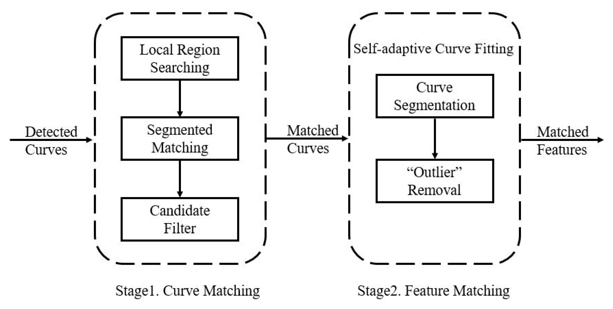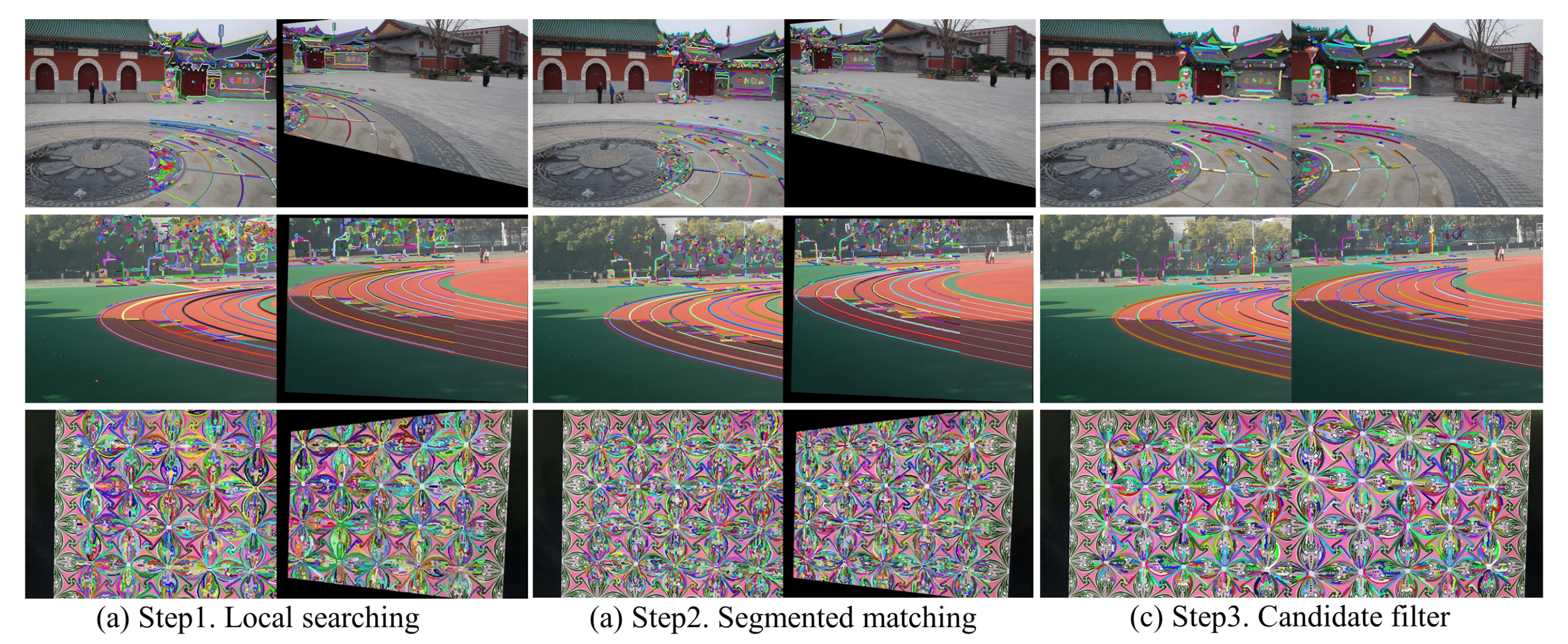Note that we use edge drawing [44] to detect curves in the images. The curve-matching stage includes three steps: local region searching, segmented matching and candidate filtering. Algorithm 1 is given to show the pseudo-code of this stage. Detailed illustrations are as follows.

Algorithm 1 The pseudo-algorithm of the curve matching stage.

Input: A pair of images $I_1$ and $I_2$ to be matched. Detect all the curves in $I_1$ and $I_2$ to obtain a curve list for each image. for each detected curve cin the curve list of $I_1$, Search c’s candidates ${\left\{c_j^{\prime }\right\}}_{j=1}^k$ in the curve list of $I_2$ by the local region searching step. for each $c_j^{\prime }$in the candidate list ${\left\{c_j^{\prime }\right\}}_{j=1}^k$, Obtain curve-segment matches on c and $c_j^{\prime }$ by executing the segmented matching step (see Algorithm 2 for details). Evaluate the curve-segment matches on c and ${\left\{c_j^{\prime }\right\}}_{j=1}^k$ to record the best-matched pairs by the candidate filtering step. Output: Accurately-matched curve-segment pairs in $I_1$ and $I_2$.

Algorithm 2 The pseudo-algorithm of segmented matching.

Input: Curve c from $I_1$ and one of its candidates in ${\left\{c_j^{\prime }\right\}}_{j=1}^k$ from $I_2^{\prime }$. Step 1. Find a pair of fiducial points on c and $c_j^{\prime }$; Step 2. Starting from the fiducial points, obtain the MSCD description of 5-pixel curve segments respectively on c and $c_j^{\prime }$, expressed as $MD{L}_c$, $MD{L}_{c_j^{\prime }}$; while$∥MD{L}_c-MD{L}_{c_j^{\prime }}∥$<${\delta }_l$, do Concatenate them to the previously matched parts as a whole, and calculate their MSCD descriptions, expressed as $MD{G}_c$, $MD{G}_{c_j^{\prime }}$; if$∥MD{G}_c-MD{G}_{c_j^{\prime }}∥$<${\delta }_g$, then Calculate the MSCD descriptions of the next 5-pixel segments for comparison. else Jump out of this iteration; Eliminate these 5-pixel segments and append the previously-matched parts to a list $L_{match}$. Go to Step 1 for the remaining parts of c and $c_j^{\prime }$. Output: Multiple curve-segment matches ($L_{match}$) on c and $c_j^{\prime }$.

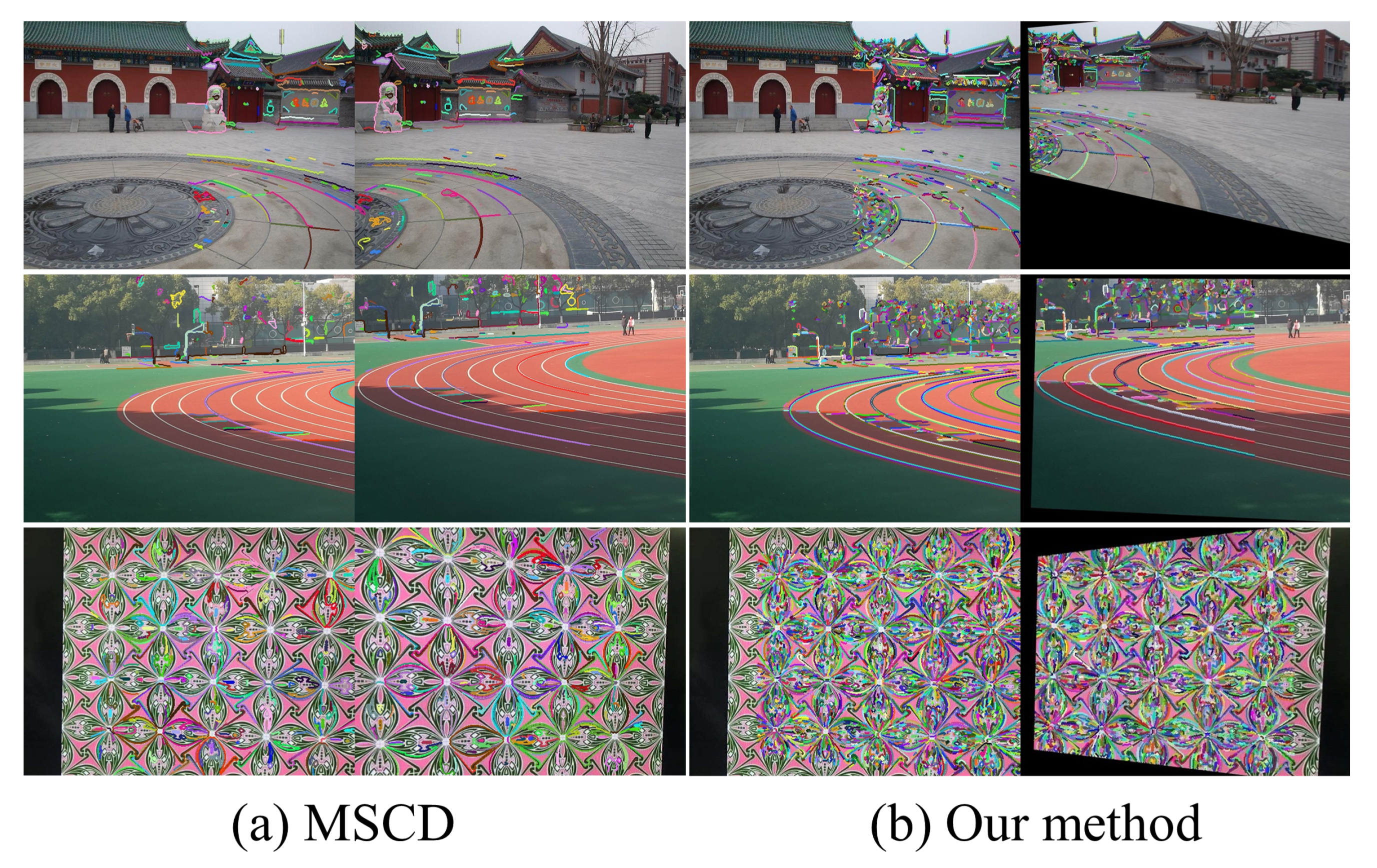
Local region searching. We project $I_2$ to $I_1$ by initial homography $H_0$ and obtain the transformed image $I_2^{\prime }$ (Figure 3c). In order to improve the precision of searching, the overlapping region in image $I_2^{\prime }$ is first partitioned into a grid of 5 × 5 cells. For each cell, an exclusive threshold, which is expressed as $max\left(ln\left({∥N_{cell}-N_{max}∥}^2\right)\times thr,thr\right)$, is adopted for candidate searching. $N_{cell}$ represents the number of keypoints in the current cell, $N_{max}$ represents the largest number of keypoints among all cells, and $thr$ is the default threshold, which is set as 2.0. The dynamic threshold can guarantee a desirable searching of curve candidates, even if the initial homography is not satisfying.

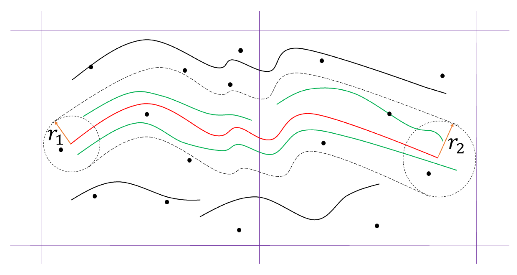
For one curve c in the overlapping region of image $I_1$, we search its potential candidates in image $I_2^{\prime }$ as follows: each pixel on c is regarded as a center, and the radius is the exclusive threshold in the corresponding cell (as shown in Figure 4). The center point slides from the starting point along c to construct the searching region in $I_2^{\prime }$; then, all the curves in this region are denoted as ${\left\{c_j^{\prime }\right\}}_{j=1}^k$. The fewer keypoints exist in a grid, the larger the searching radius will be, considering that the alignment of curves in this region is not desirable. In this way, this local searching procedure not only narrows the region of curve candidates, but also prevents the omission of potential candidates due to the changing radius.

Segmented matching. To acquire high-quality correspondences from c and its candidates ${\left\{c_j^{\prime }\right\}}_{j=1}^k$, we adopt a segmented matching strategy in this step. A pseudo-algorithm is given in Algorithm 2 to make our strategy more understood.

First, we obtain a pair of fiducial points on c and one of its candidates $c_j^{\prime }$. The fiducial points serve as the starting points of segment matching and are determined by the following procedures: (i) for each point on a curve, we describe it together with its five neighboring points on the curve under a threshold ${\delta }_f$ for the similarity of MSCD [37]; (ii) nearest/next ratio (NNDR) [13] is used to find the best matching fiducial point pair under a default NNDR ratio $\theta$.

Then, we need to match the fixed-length (set as 5 pixels in our paper) curve segments by evaluating their MSCD. Accordingly, a local threshold ${\delta }_l$ and a global threshold ${\delta }_g$ are introduced to select curve segments that have enough similarity. Starting from the fiducial points on c and $c_j^{\prime }$, the Euclidean distance of the corresponding segment’s MSCD is compared with ${\delta }_l$. Next, the matching goes on from the endpoint, and the next two 5-pixel segments are evaluated in the same manner. Then. they are joined to the matching segments as a whole to evaluate their similarity and compare it with ${\delta }_g$. The calculating and comparing is be implemented iteratively. As soon as either threshold is exceeded, the matching stops executing and we consider the joint segments matched.

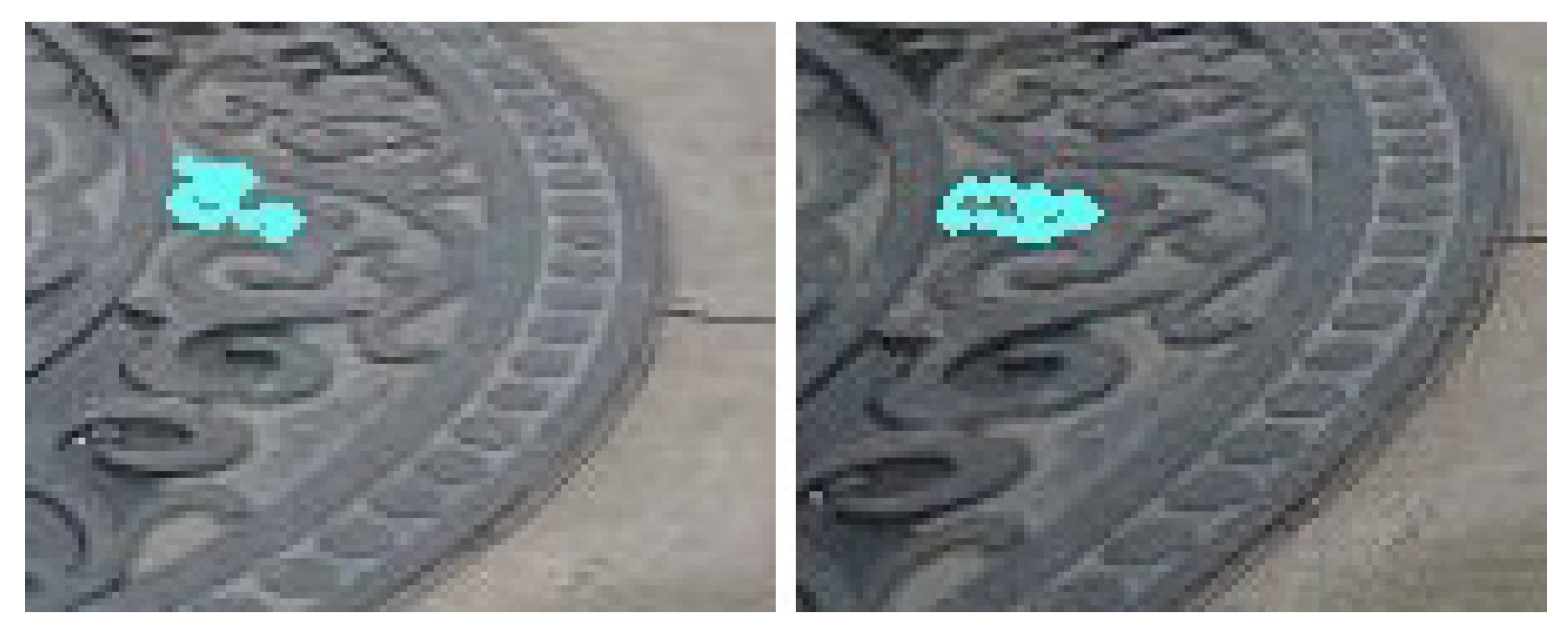
To enrich the number of correspondences, the segmented matching procedures are executed on the remaining part of curve c in the same way. That is to say, a new pair of fiducial points are obtained on the remaining curve segments, where the segmented matching algorithm will be executed again. The implementation results on one pair of correspondences are shown in Figure 5, which illustrates that multiple curve-segment matches can be obtained for one pair of curve correspondences.

As for c and all of its candidates ${\left\{c_j^{\prime }\right\}}_{j=1}^k$, the matching is implemented independently on each pair of them; namely, the segmented-matching of c is conducted n times.

Candidate filter. In this step, we need to construct an elaborate descriptor to find the best matching candidate as the unique correspondence of one curve segment. The gradient description matrix (GDM) in [37] is a widely-used descriptor for curves, which contains the most structural information in the curve neighborhood region, expressed as Equation (1), where $V_{ij}$ is used as the description vector of the sub-region $G_{ij}$. $V_{ij}$ consists of four components of the gradients distributed in the sub-region $G_{ij}$ in four directions, which are the direction of the curve, the normal direction of the curve, and their opposite directions, respectively. In addition, in Equation (1), $M_0$ and N denote the count of sub-regions and points on a curve, respectively; i ranges from 1 to $M_0$ and j ranges from 1 to N. Furthermore, based on the GDM, the MSCD is obtained by computing the normalized mean vector and the normalized standard deviation vector of the GDM’s column vectors. However, we do not find this effective enough to describe complicated irregular curves. To more accurately distinguish the candidates, we present a gradient difference descriptor (GDD) based on GDM.

$$GDM=\left(\begin{array}{cccc}{V}_{11}& V_{12}& \cdots & V_{1N}\\ V_{21}& V_{22}& \cdots & V_{2N}\\ \cdots & \cdots & \cdots & \cdots \\ V_{M_{0}1}& V_{M_{0}2}& \cdots & V_{M_{0}N}\end{array}\right)$$

(1)

$$GDD{M}_n=\left(\begin{array}{cccc}{V}_{21}-V_{11}& V_{22}-V_{12}& \cdots & V_{2N}-V_{1N}\\ V_{31}-V_{21}& V_{32}-V_{22}& \cdots & V_{3N}-V_{2N}\\ \cdots & \cdots & \cdots & \cdots \\ V_{M_{1}1}-V_{(M_1-1)1}& V_{M_{1}2}-V_{(M_1-1)2}& \cdots & V_{M_{1}N}-V_{(M_1-1)N}\end{array}\right)$$

(2)

$$GDD{M}_p=\left(\begin{array}{cccc}{V}_{\left(M_1+1\right)1}-V_{M_{1}1}& V_{\left(M_1+1\right)2}-V_{M_{1}2}& \cdots & V_{\left(M_1+1\right)N}-V_{M_{1}N}\\ V_{\left(M_1+2\right)1}-V_{\left(M_1+1\right)1}& V_{\left(M_1+2\right)2}-V_{\left(M_1+1\right)2}& \cdots & V_{\left(M_1+2\right)N}-V_{\left(M_1+1\right)N}\\ \cdots & \cdots & \cdots & \cdots \\ V_{M_{0}1}-V_{\left(M_0-1\right)1}& V_{M_{0}2}-V_{\left(M_0-1\right)2}& \cdots & V_{M_{0}N}-V_{\left(M_0-1\right)N}\end{array}\right)$$

(3)

Unlike the overall description of GDM, we adopt the gradient difference between vector $V_{ij}$ and $V_{i(j-1)}$ (or $V_{i(j+1)}$) and divide each pixel support region into positive and negative parts, as shown in Figure 6. The two matrixes are expressed as $GDD{M}_n$ and $GDD{M}_p$ in Equations (2) and (3), where $M_1=(1+M_0)/2$. Accordingly, two vectors of the gradient difference descriptor can be calculated to describe each side of the curve, thus helping to find the unique corresponding curve in $I_2^{\prime }$. Then, we project it back to $I_2$ to obtain $c^{\prime }$, which is the unique correspondence of c.

The above illustration focuses on one curve and its candidates to explain the procedures of curve matching. With all the curves in the image pair implemented according to the same procedures, a set of curve matches ${\left\{c_i,c_i^{\prime }\right\}}_{i=1}^m$ can be obtained in the curve-matching stage.

The whole curve-matching stage provides us curve pairs that have been matched as accurately as possible. Next, we need a further stage to extract the invariant features from the matched curves to make good use of them.

3.2. Feature Matching

The potential matching curves of the same object from different views should be the “same”, with one projective transformation between them. However, due to changes of perspective and pixel-level description, two curves in a pair may still have minor differences. In our paper, a curve-fitting approach is adopted to eliminate the diversities.

However, if we directly implement curve fitting on the curve pairs obtained in Section 3.1, it is not enough to fit the curves well, which would influence the extraction of invariant features. Therefore, a self-adaptive fitting strategy is proposed to fit the curves more accurately, which includes self-adaptive segmentation and “outlier” removal under the constraint of fitting error.

As proven in the Appendix A, the maximal curvature point is translation, rotation, and scale invariant, making it a proper feature of a fitted curve. Since the curvature $k=\left|y^{″}\right|/{(1+{y^{\prime }}^2)}^{\frac{3}{2}}$ depends on the second derivative of the curve, any form of curve function that has the second derivative can be employed to extract the maximal curvature points. For convenience, we employ the cubic polynomial $f(a,b,c,d;x)=a{x}^3+b{x}^2+cx+d$ to fit the matched curves. Hence, we calculate the fitting error between $f(a,b,c,d;x)$ and the curve as the segmentation and outlier removal criteria, which can be expressed as $RMSE\left(f\right)=\sqrt{\frac{1}{N}{\sum }_i^N{∥y_i-f(a,b,c,d;x_i)∥}^2}$. The curve-fitting threshold is set as ${\epsilon }_c$, which controls the curve segmentation and the outlier removal at the same time.

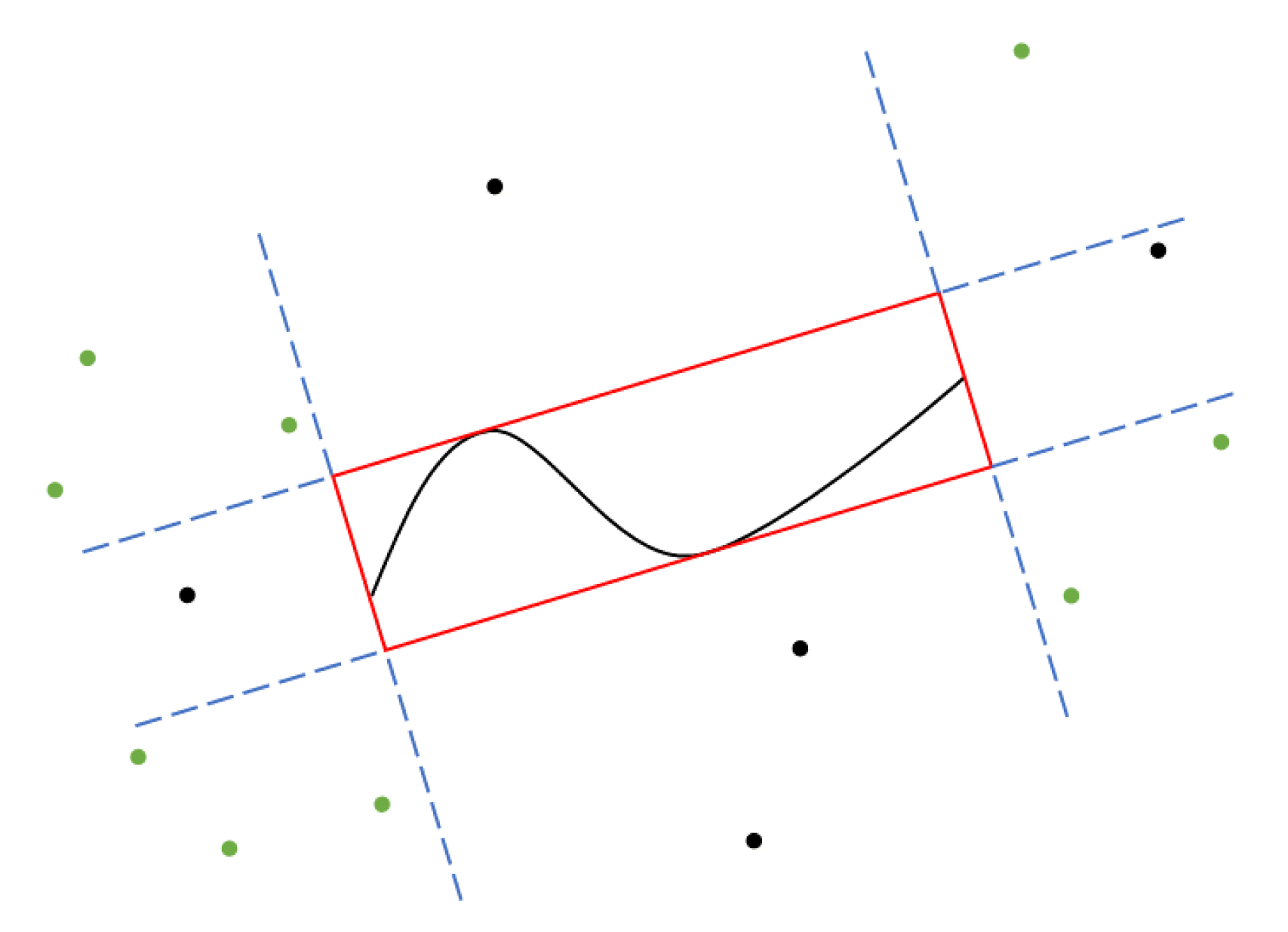
Self-adaptive segmentation. The detected keypoints in an image can provide a strong constraint for their enclosing region, which encourages us to choose the surrounding keypoints of a curve to constrain the curve fitting and matched-feature extraction. Figure 7 shows the explanation of the surrounding keypoints.

The objective function to estimate the invariant features for a pair of curve segments is expressed as:

$$E=E_{fitting}+E_{feature}+E_{keypoint},$$

(4)

where $E_{fitting}$ is the curve fitting term, $E_{feature}$ is the feature extracting term, and $E_{keypoint}$ is the surrounding keypoint constraint term. The $E_{fitting}$ is used to evaluate the fitting of curve matches $(c_i,c_i^{\prime })$ and is defined as:

$$E_{fitting}=\sum _{i=1}^{N_1}(f_1\left(x{1}_i\right)-y{1}_i)+\sum _{j=1}^{N_2}(f_2\left(x{2}_j\right)-y{2}_j),$$

(5)

where $f_1(a_1,b_1,c_1,d_1;x1)$, $N_1$ and $(x{1}_i,y{1}_i)$ represent the curve fitting function and the number of pixels and pixel coordinate of $c_i$, respectively, while $f_2(a_2,b_2,c_2,d_2;x2)$, $N_2$ and $(x{2}_j,y{2}_j)$ describe $c_i^{\prime }$, accordingly.

The maximal curvature points serve as the features of the fitting curve, and the local homography $h_l$ estimated by the surrounding keypoints is used to align the corresponding curve segments. There also exists a projective transformation between the matching maximal curvature points on the fitting curves, so the feature extracting term $E_{feature}$ is:

$$E_{feature}=\sum _{i=1}^{N_c}{∥{\tilde{p}}_{c_i}-h_l{\tilde{p}}_{c_i}^{\prime }∥}^2,$$

(6)

where $p_{c_i}\leftrightarrow p_{c_i}^{\prime }$ is a pair of maximal curvature points that are the invariant features we expect to obtain, and $N_c$ is the number of the invariant feature matches.

We resort to the surrounding keypoints as another kind of constraint. The constraint term of keypoints $E_{keypoint}$ can be written as:

$$E_{keypoint}=\sum _{i=1}^{N_f}{∥{\tilde{p}}_{f_i}-h_l{\tilde{p}}_{f_i}^{\prime }∥}^2,$$

(7)

where $p_{f_i}\leftrightarrow p_{f_i}^{\prime }$ is a pair of surrounding keypoints and $N_f$ is the number of matches.

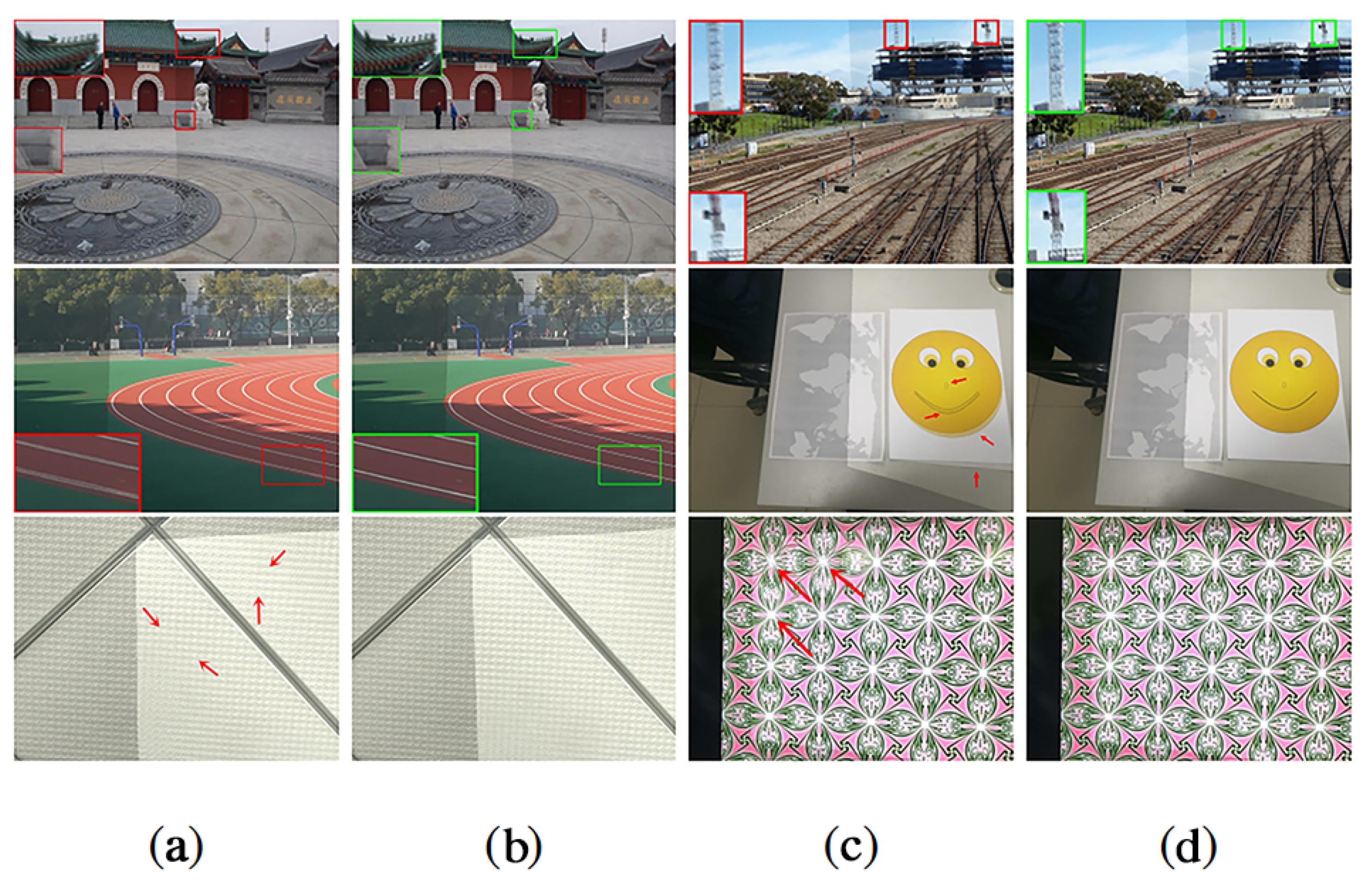
Outlier removal. During the process of curve fitting, some defective points exist that would disturb the error calculation if added, which are regarded as the “outliers” in our paper. To this end, we evaluate the RMSE of the fitted curves to remove those points. The outlier removal process is executed along with the optimization of the objective function. In the ablation study of Section 4.5, we can notice that the number of final matched features increases when adding our “outlier” removal operation.

Please note that our outlier-removal process is quite different from conventional methods such as RANSAC [26]. These methods often serve as a post-processing procedure and aim to remove some poorly-matched points that would reduce the number of final matches. Conversely, our outlier removal aims to remove the defective points that would affect the curve fitting performance, which contributes to the whole optimization of our fitting process and further boosts the quality and quantity of the extracted features.

Ultimately, the selection of maximal curvature points of $c_i$ and $c_i^{\prime }$ are determined by a RMSE threshold ${\epsilon }_{inv}$. According to the procedures above, a set of matching features ${\left\{p_{c_i},p_{c_i}^{\prime }\right\}}_{i=1}^Q$(Q represents the number of matched maximal curvature point pairs) from the curve pair ${\left\{c_i,c_i^{\prime }\right\}}_{i=1}^m$ can be obtained.

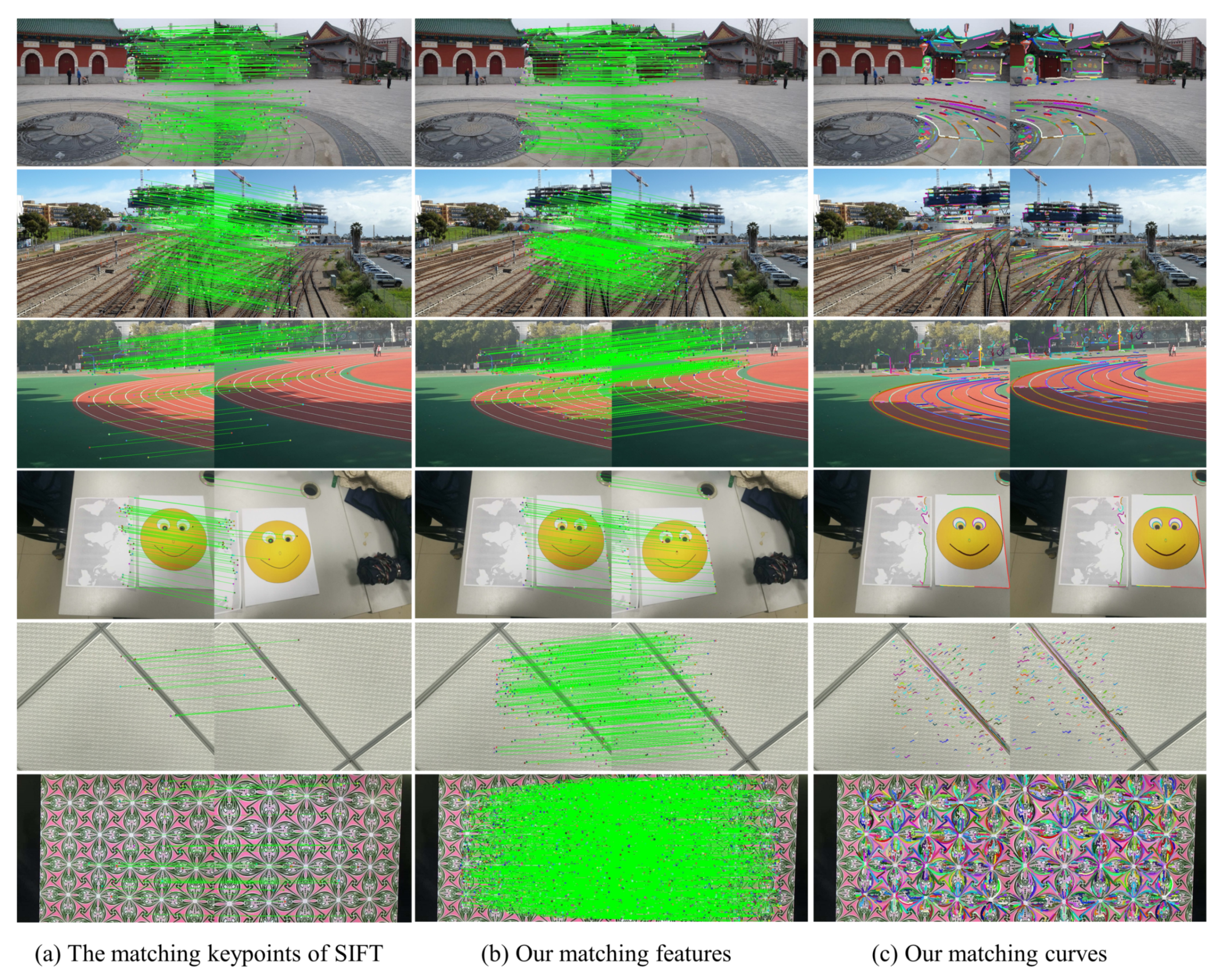
Note that conventional methods are relatively weak in dealing with two situations: (1) in low-texture scenes, keypoints cannot be detected easily, which directly influences feature matching; (2) in repeated-texture scenes, although keypoints can be detected, the following feature matching is quite difficult due to the similarity of descriptions. Therefore, an insufficient number of keypoints may lead to an unsatisfactory homography and perspective transformation. When using our elaborate matching steps, the matching of our invariant features derived from the curve is not be affected.

4. Experimental Results and Analysis

4.1. Parameters

As a method of local matching and fitting, several parameters are used in our experiments. However, the process of our end-to-end method is based on fixed values of parameters and executed automatically, with no extra handcrafted procedures needed. The three emphasized parameters in

Table 1. The parameter settings for the thresholds in our experiments. ${\delta }_f$: fiducial point matching; $\theta$: NNDR ratio; ${\delta }_l$: local segmented matching; ${\delta }_g$: global segmented matching; $\delta$: candidate filter; ${\epsilon }_c$: curve segmentation and outlier removal; ${\epsilon }_{kp}$: surrounding keypoints selection; ${\epsilon }_{inv}$: feature matching.

Parameter	Value	Parameter	Value
${\mathbf{\delta }}_{\mathbf{f}}$	0.55	$\theta$	0.6
${\mathbf{\delta }}_{\mathbf{l}}$	0.65	${\delta }_g$	0.55
$\delta$	0.3	${\epsilon }_c$	1.0
${\epsilon }_{kp}$	0.5	${\mathbf{\epsilon }}_{\mathbf{inv}}$	1.0

are related to the distribution and the matching precision of the invariant features. Therefore, these parameters can be slightly adjusted to obtain a better result in practical use.

As stated in above sections, the intention of our method is to extract accurately-matched feature points from irregular curves. Thus, we choose methods that focus on point features, including classic and modern techniques. The baselines in our experiments are classic methods, i.e., SIFT [13], SURF [20], ORB [14], BRISK [23], and deep-learning methods, i.e., LIFT [48], SuperPoint [45], and LF-Net [47].

We use Vlfeat [49] to implement keypoint extraction for SIFT, with the peak threshold and edge threshold set as 0 and 10, respectively. For other traditional methods such as ORB, SURF, and BRISK, we use the detection implementation provided by OpenCV. Brute-force Matcher is used for keypoint matching, and RANSAC [26] is used to remove the mismatches for these methods. As for the deep-learning based methods—LIFT, SuperPoint and LF-Net—we use the source code on Github released by their authors.

4.2. Implementation Details

This part briefly describes the implementation details of our experiments. The programs of our approach as well as the classic methods are implemented on Intel I5-6400 and NVIDIA GTX 1050 with 2GB memory. Our program is based on C++ and is developed with Visual Studio 2017. The development environment includes OpenCV 3.0 and Eigen 3.2.0 for image processing and matrix and vector operations. In addition, Vlfeat [49] and Edge Drawing [44] are used for keypoint extraction and curve detection, respectively, and the Levenberg–Marquardt programming method [50] is used to optimize the objective function. The deep-learning models are evaluated on a single NVIDIA RTX 2080Ti GPU using the published code released by the authors.

4.3. Datasets

The images used in our experiment are divided into three scenes: ordinary scenes, low-texture scenes, and repeated-texture scenes. The ordinary scenes temple and railtrack were used in paper [4]. The low-texture scenes playground, table, and repeated-texture scenes roof are captured by us. The repeated-texture scene pattern was downloaded from the Internet. All the images used in our paper can be obtained from this website for future comparisons (https://github.com/davidyinnan/curve accessed on 22 February 2022). In addition, the datasets used for relative pose estimation and feature-based image searching in Section 4.7 were acquired from TUM [51].

4.4. Analysis of Curve Matching

To match curves abundantly and accurately, in the curve-matching stage, we implement three steps following the order presented in Section 3.1. Note that, it is essential for curve matching to perform these three steps in this order. For example, the second step should be executed before the third; otherwise, a large number of the potential curve matches will be rejected by GDD, leading, resulting in missed correspondences. For clarity, the output of each step of this stage is shown in Figure 8. Furthermore, we conducted the following experiments on the ordinary scene temple to analyze the necessity of each step.

First, we intended to illustrate the importance of local region searching. It is obvious in Figure 9a that the two curves are mismatched, while the result of using local region searching manifests better performance, as shown in Figure 9b.

After local region searching, we may still obtain some mismatches under a large threshold, as shown in Figure 9c. However, using a stricter threshold may cause us to miss many potential curve pairs. However, with our segmented matching step, more abundant and correct matches can be obtained even under a strict threshold, as shown in Figure 9d.

The next comparison was conducted to prove the effect of GDD on filtering curve candidates. Following the first two steps, if GDM is used for description, more than one matching curve may be obtained, as shown in Figure 9e. Figure 9f demonstrates the correct matching using our presented GDD.

More comparisons to MSCD curve matching are shown in Figure 10. We can observe that there exist extensive mismatches when directly adopting MSCD, where two curves are considered matched as long as the Euclidean distance of their descriptors is below a threshold. In contrast, we present a local and elaborate strategy to match the curves as accurately as possible, and the results are satisfying.

For scenes of different textures, Figure 11c shows the curve-matching results with our curve-matching strategy. It is obvious that our method is able to obtain abundant curve matches, especially in the low-texture scenes playground and table, as well as in the repeated-texture scenes roof and pattern. Besides, these curve correspondences are matched as accurately as possible. Note that there might exist mismatches for twisted curves in sophisticated regions (see Figure 12), but such mismatches can be eliminated in the next stage of our approach.

4.5. Analysis of Feature Matching

To accurately extract the invariant features from curves, we adopt a self-adaptive fitting strategy for feature matching. We also resort to the strong constraint of the surrounding keypoints to obtain the matching maximal curvature points. In the following comparisons, we continue to use the temple scene for illustration.

As we mentioned in Section 1, the second reason why it is difficult to match the detected curves directly is the pixel distribution change. Points on the detected curves are described based on discrete pixels, which makes it quite unpractical to obtain the matching maximal curvature points. To show the significance of curve fitting, we attempt to extract the maximal curvature points from two corresponding curve segments. As clearly shown in Figure 13, the extracted points cannot match with each other, which calls for a curve-fitting strategy to eliminate the disturbance of pixel-level descriptions caused by curve detection.

Self-adaptive curve fitting. There are several key procedures for our proposed curve fitting, including curve segmentation, outlier removal, and the constraining of surrounding keypoints. All of these procedures make great contributions to the extraction of invariant features. In this part, we conduct ablation experiments to show the importance of these procedures. For each factor removed, the number and accuracy of the extracted features were recorded and compared. The accuracy is evaluated by the RMSE of the maximal curvature point matches ${\left\{p_{c_i},p_{c_i}^{\prime }\right\}}_{i=1}^Q$, where $p_{c_i}^{\prime }$ is the corresponding point of $p_{c_i}$ after mapping of the initial homography. Note that when we remove the constraint on the surrounding keypoints, we use all the keypoint matches in the whole image as the constraint for comparison.

As shown in

Table 2. The ablation study for the self-adaptive curve fitting. The best results are marked in bold.

Method	Number ↑	RMSE ↓
W/o curve segmentation	313	3.0941
W/o “outlier” removal	199	2.9772
W/o surrounding keypoints	286	2.8371
Ours	330	2.6913

, the metric results degrade if any of the three factors are removed, indicating the significance of the curve segmentation, outlier removal, and constraining of surrounding keypoints. Besides, it can also be noticed that our outlier-removal operation is not the same as in classic outlier-removing methods. Instead of removing the poorly-matched points and reducing the number of final matches (e.g., RANSAC [26]), our outlier-removal strategy is to remove the defective points that would affect the curve fitting performance. Therefore, when executing outlier removal, the number of final matched features increases accordingly, indicating that the whole fitting is well conducted and optimized.

We also conducted experiments to prove that the effectiveness of our method is not be limited by the form of the fitting function, as shown in

Table 3. Performance on various scenes with different polynomial fitting functions.

Texture	Scene	Cubic		Quartic		Quintic
		Number	Error	Number	Error	Number	Error
Ordinary	Temple	314	2.837	409	2.917	461	2.885
	Railtrack	464	3.908	472	3.988	406	4.082
Low-texture	Playground	329	2.009	506	2.542	453	2.365
	Table	76	2.034	81	2.149	78	2.114
Repeated-texture	Roof	328	2.517	408	2.518	334	2.603
	Pattern	1618	4.256	1801	4.512	1842	4.163

. We evaluated the number and the RMSE of the extracted features using different fitting forms: cubic, quartic, and quintic polynomials. The extracted features are sufficient no matter which polynomial is adopted, and the errors remain stable as well. This proves that our method is not limited by the form of the fitting function.

Feature matching. Since the ultimate goal of our method is to accurately match the features derived from curves, we conducted experiments to show the superiority of our method in comparison with the baselines, including the classic approaches (SIFT, ORB, SURF, and BRISK) and the deep-learning techniques (LIFT, SuperPoint, and LF-Net). The six pairs of input images were divided into three groups of different textures: ordinary, low-texture and repeated-texture. The matching number of the features extracted by different methods are compared in

Table 4. The matching numbers and processing times using different approaches in various scenes. Best results are marked in bold.

	Ordinary		Low-Texture		Repeated-Texture
	Temple	Railtrack	Playground	Table	Roof	Pattern
SIFT [13]	279	353	143	64	25	40
SURF [20]	291	381	135	68	33	73
ORB [14]	264	372	121	49	20	57
BRISK [23]	284	359	160	57	19	67
LIFT [48]	298	377	190	67	134	245
SuperPoint [45]	318	427	203	45	162	311
LF-Net [47]	269	435	256	68	276	477
Ours	314	464	329	76	328	1618

.

Comparisons with classic methods. Our method manifests significant superiority over classic methods; to be specific: (1) in ordinary scenes, our method is quite comparable to all the baselines; (2) in low-texture scenes where the baselines cannot detect enough feature points, the ultimate matching number of their results is not optimal, while our method can still extract a large quantity of matched features; (3) in repeated-texture scenes, traditional methods can detect enough keypoints, yet may fail to acquire rich matches due to the similarity of the descriptors.

Comparisons with deep-learning methods. As for the deep-learning-based methods, training datasets for neural networks are limited, but the analytical method that we present does not need training datasets at all. Conversely, our approach pays attention to the structural details of an image, namely, the detected irregular curves. By the proposed self-adaptive curve fitting strategy, rich point matches can be extracted from the accurately matched curve segments. Although these methods can extract comparable feature points to classic methods, our algorithm shows better performance in low-texture and repeated-texture scenes, as we focus on accurately extracting features from the widely-existing curves in the image.

Qualitative comparisons. Since the baselines focus on detecting features from the whole image, we choose SIFT as the representative method for qualitative demonstration. Figure 11 provides a clear comparison of the matching points by SIFT and our method. We can notice that in areas such as the runway in playground and the smiling-face picture in table, where textures and lines are both lacking, rich curves can be matched by our method, thus contributing to a better distribution of our features compared to SIFT keypoints. With regard to the repeated-texture images roof and pattern, our method can extract a larger number of matching features with better distribution compared to SIFT.

4.6. Analysis of Processing Time

As for the specific running time for each stage of our method, the details are shown in

Table 5. The processing time of each stage on different scenes.

Texture	Scene	Curve-Matching Time (s)	Feature-Matching Time (s)	Image Size
Ordinary	Temple	55	26	730 × 487
	railtrack	69	49	720×540
Low-texture	Playground	48	23	720 × 540
	Table	7	16	1440×1080
Repeated-texture	Roof	63	21	720 × 540
	Pattern	96	27	600×450

. The computational efficiency of our algorithm highly depends on the resolution of the input image, as well as the textures in it. A higher resolution or a larger number of detected curves indicates a longer implementation time. To boost the implementation speed of the self-adaptive curve fitting, we evaluate the Jacobian terms of the objective function defined in Equation (4) and optimize the objective function using the Levenberg–Marquardt programming method [50], which helps the solution converge more rapidly.

4.7. Applications

In this part, we show the comparisons of our method and SIFT on image stitching and relative pose estimation. We also conduct a simple application of feature-based image searching.

Image stitching. We compared the alignment quality of image stitching using our features and SIFT keypoints, which are based on a classic stitching model APAP [4] and are evaluated by local similarity in the overlapping regions. For each alignment, we used the same accuracy measurement in [30]. For pixels in the overlapping region, we used a 3 × 3 window to calculate the RMSE of one minus normalized cross correlation (NCC), i.e., $RMSE(I_i,I_j)=\sqrt{\frac{1}{N}{\sum }_{\pi }{∥1-NCC(x_i,x_j)∥}^2}$, where N is the number of pixels in the overlapping region $\pi$, and $x_i$ and $x_j$ are the pixels in image $I_i$ and $I_j$, respectively.

Figure 14 shows the stitching results using keypoints and our features. As we zoom in, it can be observed that the stitching quality based on our features is apparently higher than using keypoints. There are multiple ghosting artifacts in the results using SIFT keypoints, while our results show desirable alignments in the overlapping regions. Moreover,

Table 6. The pixel RMSE ([0, 255]) of SIFT keypoints and our invariant features in each image pair. Best results are marked in bold.

Scene	SIFT	Ours	Scene	SIFT	Ours
Temple	5.55	5.09	Railtrack	13.41	11.81
Playground	8.39	5.81	Table	2.77	2.41
Roof	4.10	3.84	Pattern	29.15	26.71

shows RMSE results using keypoints and our extracted features. The higher stitching quality and the smaller alignment errors of our results indicate that our extracted features accurately match and have good distribution, which can significantly contribute to the application of image stitching. More comparisons about image stitching are shown in Figure 15d,e.

Relative pose estimation. In this experiment, we showed the application in relative pose estimation using our extracted features as a complement for SIFT keypoints. We used three RGB datasets with different textures, which were acquired from TUM [51] since it can provide the intrinsic parameters and the ground truth trajectory of the camera. We randomly chose a frame and the thirtieth frame after it; then, we evaluated the rotation matrix and translation vector between these two frames based on the classic 5-point algorithm [9]. After that, we compared the rotation and translation angle between the estimated vector and the ground truth data as the error of estimation. The average error of 50 groups of images was calculated and demonstrated for each scene.

As shown in

Table 7. The accuracy results of relative pose estimation. Best results are marked in bold.

Data	Points	Avg. Error of R	Avg. Error of T
Picture	SIFT	1.1589	3.2564
	Ours	1.2350	4.1220
	Both	0.5563	1.8952
Bear	SIFT	1.3720	1.7954
	Ours	1.3596	1.7258
	Both	0.8962	0.8841
Ball	SIFT	1.1080	5.2665
	Ours	1.8141	6.3214
	Both	1.0245	5.2533

, in scenes picture and bear, the accuracy of estimation by our method is quite comparable to that of SIFT keypoints, but our results on ball are not satisfying, as the detected curves are not enough. What is more, when we further combine our features and keypoints together to estimate the relative pose of the camera, accuracy can be improved. Hence, our extracted invariant features are quite precise and can also serve as a powerful complement to existing keypoints to improve the accuracy of estimation. The extracted features of each scene are shown in Figure 16.

Feature-based image searching. We conducted a simple application of feature-based image searching using the matching features extracted by our method, as shown in Figure 17. The frame sequences were also from datasets on TUM. For the two videos picture and bear, we sampled the images ten frames after another. For the mixed test, we randomly chose five samples from picture and bear. We can observe that the matching number of the features degrades when the perspective becomes larger or the scene is changed, which shows that the features extracted from curves by our method can be used to evaluate the similarity between images and to search for similar ones.

5. Discussions and Limitations

Curve missing. In ordinary and repeated-texture senses, it is possible to detect multiple curves. However, in some low-texture environments, the number of detected curves is limited, which is the same as with feature points. Especially when a covering object appears or a curve is projected as a straight line in an image, there is a lack of curves to match. In these cases, it is difficult to accurately match curves with large shape differences in the curve-matching stage, so the number of extracted curve features decreases accordingly.

Perspective changes. As the difference of viewing perspective turns larger, the detected curves of the same object in two images are more likely to manifest different appearances, thus making our second stage—feature matching—more difficult to execute. However, as we illustrate in Section 3.2, most of the outlier points can be effectively removed by using our self-adaptive curve-fitting strategy without affecting the matching accuracy.

Implementation time. Although the matching numbers of our algorithm are exceedingly superior to the state-of-the-art methods, the processing time remains to be a limitation of our method. The relatively long implementation time is due to the multi-stage dealing of matching curves and extracting features. The more curves are detected, the more time our method takes.

6. Conclusions

In this paper, we tackle the bottleneck problem of feature detection and feature matching in environments where feature points and line structures are both lacking. An effective method is proposed to match invariant features derived from irregular curves, which consists of two stages: curve matching and feature matching. Our method is able to match irregular curves accurately. Moreover, to make better use of these matched curves, we also propose to extract a large set of features from them, which can be applied in various environments, especially low-texture and repeated-texture scenes. Extensive experiments showed the effectiveness of our method both quantitatively and qualitatively.