Article

Flood Monitoring Using Enhanced Resolution Passive Microwave Data: A Test Case over Bangladesh

1
Department of Civil, Environmental, Architectural Engineering and Mathematics, University of Brescia, Via Branze 43, 25123 Brescia, Italy
2
Lamont-Doherty Earth Observatory, Columbia University, 61 Rte 9W, Palisades, NY 10964, USA
3
NASA Goddard Institute of Space Studies, 2880 Broadway, New York, NY 10027, USA
4
School of Geography, Development, and Environment, University of Arizona, 1064 E. Lowell Street, Tucson, AZ 85721, USA
5
Cloud to Street, New York, NY 11201, USA
*
Author to whom correspondence should be addressed.
Remote Sens. 2022, 14(5), 1180; https://doi.org/10.3390/rs14051180
Submission received: 18 January 2022 / Revised: 21 February 2022 / Accepted: 22 February 2022 / Published: 27 February 2022

Abstract

:
Monitoring floods is a major issue in water resources management and risk mitigation, especially in the Global South. Optical and radar observations, even providing a fine spatial resolution, are still limited by cloud cover interaction or insufficient temporal resolution. On the other hand, passive microwave (PMW) sensors collect information on a daily frequency with minor cloud cover interaction, but they have been historically limited in terms of spatial resolution. Here, we evaluate the capability of an enhanced spatial resolution PMW dataset (3.125 km) in monitoring spatio-temporal evolution of flood events, focusing on a major flood event that occurred in October 2005 in Bangladesh. We apply an algorithm aimed to remove the seasonal variability of surface temperature from the PMW timeseries, exploiting the difference in emissivity between dry and water-covered pixels. We assess the capability of the algorithm in capturing flood evolution and extension through the comparison with quantities obtained from optical data collected by the Moderate Resolution Imaging Spectroradiometer (MODIS) and water level measurements. We also compare the enhanced product with the historical coarser resolution dataset by means of a variogram-based analysis to evaluate the improvements in terms of spatial representation. Finally, we evaluate the possibility to extract the water fraction within a single pixel by using an Advanced Microwave Scanning Radiometer—Earth Observing System (AMSR-E) emissivity dataset and compare the estimates with MODIS-derived water fractions. Our results show that the enhanced PMW product outperforms the coarser one when compared to flood mapped from optical data based on information content, indicating that it is possible to integrate such a product into the mapping of floods at a global scale on a daily basis.

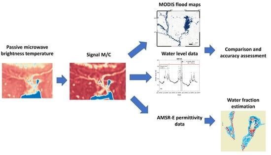
Graphical Abstract

1. Introduction and Background

Flooding is a frequent hydrologic hazard, affecting everyday life and impacting social and economic systems, especially in the Global South. Structural and non-structural mitigation measurements should be based on proper knowledge of the spatial and temporal evolution of such devastating events. In this regard, the increase in the availability of radar and optical spaceborne data in recent years has allowed monitoring the spatial distribution and temporal evolution of floods with increased accuracy with respect to the previous decades [1,2,3]. Despite this, however, several major issues need to be addressed for properly capturing the spatio-temporal evolution of floods, especially in regions where in situ measurements and data infrastructures are not well developed and readily available, as in the Global South. While optical data are routinely collected at high spatial (~meters or tens of meters) and temporal (daily) resolutions, the presence of clouds within the acquired scene can often obstruct the view of the sensors, especially during floods associated with hurricanes and heavy rain. On the other hand, radar data are not limited to clear sky conditions and can collect information during cloudy conditions and without the need for solar illumination. However, current available radar datasets are characterized by a relatively coarse temporal resolution (6–12 days in the case of Sentinel-1 sensors depending on year and location) and short record (~2015–present), introducing strong limitations in monitoring the short-term evolution of floods. While radars mounted on small satellites are becoming more popular, they are still cost-prohibitive and not yet currently available at a daily timestep. Moreover, acquisitions must be tasked, limiting their access to a wide audience of researchers and utility for flood monitoring.
A complementary approach to optical and radar sensors consists of using passive microwave (PMW) data. While radars collect information of the scene under observation in an active way, PMW sensors measure the electromagnetic radiation naturally emitted by the Earth. Because of their large swath (of the order of a thousand kilometers), PMW sensors can collect useful information over most of the Earth at high temporal resolution (daily or even sub-daily, depending on the latitude), representing a strong candidate for long-term, high temporal resolution detection of floods or their mapping. Building on the sensitivity of PMW data to dry and wet surfaces [4], several algorithms have been proposed in the past that aim at mapping floods using PMW data [5,6,7,8,9,10,11,12,13,14,15]. One of the first assessments of PMW sensors’ capability of monitoring floods was carried out by Allison et al. [11], using data at 19.3 GHz collected by the Electrically Scanning Microwave Radiometer (ESMR) Nimbus-5 satellite. However, as we mentioned, there is a temporal gap between the ESMR data and the next available PMW sensor, the SMMR launched in 1979. Later, Giddings, and Choudhury [12] used both horizontally and vertically polarized brightness temperatures at 37 GHz collected by the Nimbus-7 SMMR to monitor seasonal inundation in South America through the so-called polarization difference, defined as the difference between vertically and horizontally polarized brightness temperatures. Similarly, following Choudhury [13], Sippel et al. [6] used the polarization difference to assess the inundation area in the Amazon River floodplain. In the early 2000s, a different methodology was proposed by Galantowicz [7] in which the 19 GHz and 37 GHz horizontally polarized brightness temperatures and a digital elevation model are combined for flood mapping purposes. Prigent et al. [14] used 37 GHz SSM/I emissivity (obtained removing the influence of the atmosphere, clouds and rain) together with ERS-1 active microwave scatterometer data (sensitive to vegetation density) and the AVHRR Normalized Difference Vegetation Index to capture global wetland dynamics to create the Global Inundation Extent from Multi-Satellites (GIEMS).
If we exclude the Electrically Scanning Microwave Radiometer (ESMR) aboard NOAA’s Nimbus-5 satellite which was launched in 1972 but was acquiring data only for a short period, the first satellite to start collecting PMW brightness temperatures without temporal gaps was launched in 1979, carrying the Scanning Microwave Multichannel Radiometer (SMMR), followed by the Special Sensor Microwave/Imager (SSM/I, since 1987) and the Special Sensor Microwave Imager/Sounder (SSMI/S, since 2006) flying on the Defense Meteorological Program Satellites (DMSP 5D-2/F8, F10, F11, F13, F14, DMSP 5D-3/F15 for SSM/I and DMSP 5D-3/F16, F17, F18, F19 for SSMI/S). A major limitation of the historical approaches making use of PMW data consists of the relatively coarse spatial resolution at which these datasets have been produced and distributed (25 km). In this regard, a new “spatially enhanced” dataset was recently produced within the framework of a NASA MeEASUREs Project [16], containing calibrated PMW brightness temperatures at spatial resolutions of 3.125 km, 6.25 km, 12.5 km, and 25 km for the period 1979–2019 from all available sensors. The enhancement of the spatial resolution is achieved at the cost of a potential increase in the noise in the final product. It is, therefore, important to assess the impact of such noise on the use of the enhanced product in flood detection.
In this paper, we apply the algorithm developed by De Groeve [5] to the enhanced PMW brightness temperatures at 37 GHz (3.125 km) to assess the skills of the new product to map floods. To perform our assessment, we focus on an area in Bangladesh during a major flood event that occurred in October 2005. For assessing the performance of the enhanced PMW product to map the spatio-temporal variability of the flood under study, we compare the results obtained with the enhanced PMW product with those obtained from the same dataset at the historical, coarser resolution (25 km) and with those obtained from the analysis of optical data collected by the Moderate Resolution Imaging Spectroradiometer (MODIS) at the spatial resolution of 500 m over a portion of the study area. Building on the finer spatial resolution of MODIS data, we also conduct a sensitivity analysis of the skills of the enhanced PMW product to map the surface water fraction (here defined as the relative portion of the area pixel where the flood is occurring). Such a comparison is aimed at quantifying possible improvements related to the enhancement of spatial resolution of the dataset. We continue evaluating the capability of the PMW algorithm outputs in describing the temporal evolution of the flood event by comparing them with water level data measured by a selected hydrometric station. Then, we report the results of a semi-variograms analysis to study the scale lengths and the spatial autocorrelation of the PMW and MODIS-based products [17], aiming at evaluating the consistency of the PMW datasets with respect to the higher resolution MODIS reference. Lastly, we make use of a global permittivity dataset to retrieve the water fractional area within each PMW pixel and compare it with that obtained with MODIS.

2. Materials and Methods

2.1. Study Area

Our study area covers Bangladesh and East India, and it is bounded by the following latitude and longitude values: 20.9905°N–28.8737°N and 81.8462°E–95.0090°E, for a total surface area of 1,164,600 km2. The region is confined in the north by the Himalayan Mountains and in the south by the Bay of Bengal (Figure 1). The three major rivers draining the Bangladesh basin are Ganges, Brahmaputra, and Meghna. The hydrologic response of this colossal river system is triggered by monsoon rainfall, meltwater from the Himalayas, and tides at the delta. Whenever an increment of runoff from the three tributaries occurs, strong flood events affect the downstream river system [18]. Moreover, the area is exposed to floods from cyclones, such as the super cyclone Amphan that hit the area at the beginning of June 2020 and was the strongest cyclone recorded in the area, with winds reaching ~160 miles per hour. A total of 1.4 billion people inhabit this active river delta, including the megacity of Dhaka, rural areas with extensive agriculture and especially rice cropping, and the UNESCO world heritage site of the Sundarbans mangrove forest. We specifically focus our attention on a flood event that occurred between 3 and 17 October 2005, when dozens of villages were inundated by extreme rainfall, causing the rivers of northwestern Bangladesh to burst their banks. The flood lasted for at least 20 days, killing 19 people, displacing ~100,000 people, and affecting an estimated area of ~23,000 km2. The flood was associated with late monsoon rains, damaging 200,000 hectares of crops and leaving 10,000 homeless families in the Rangpur region alone.

2.2. Passive Microwave Data

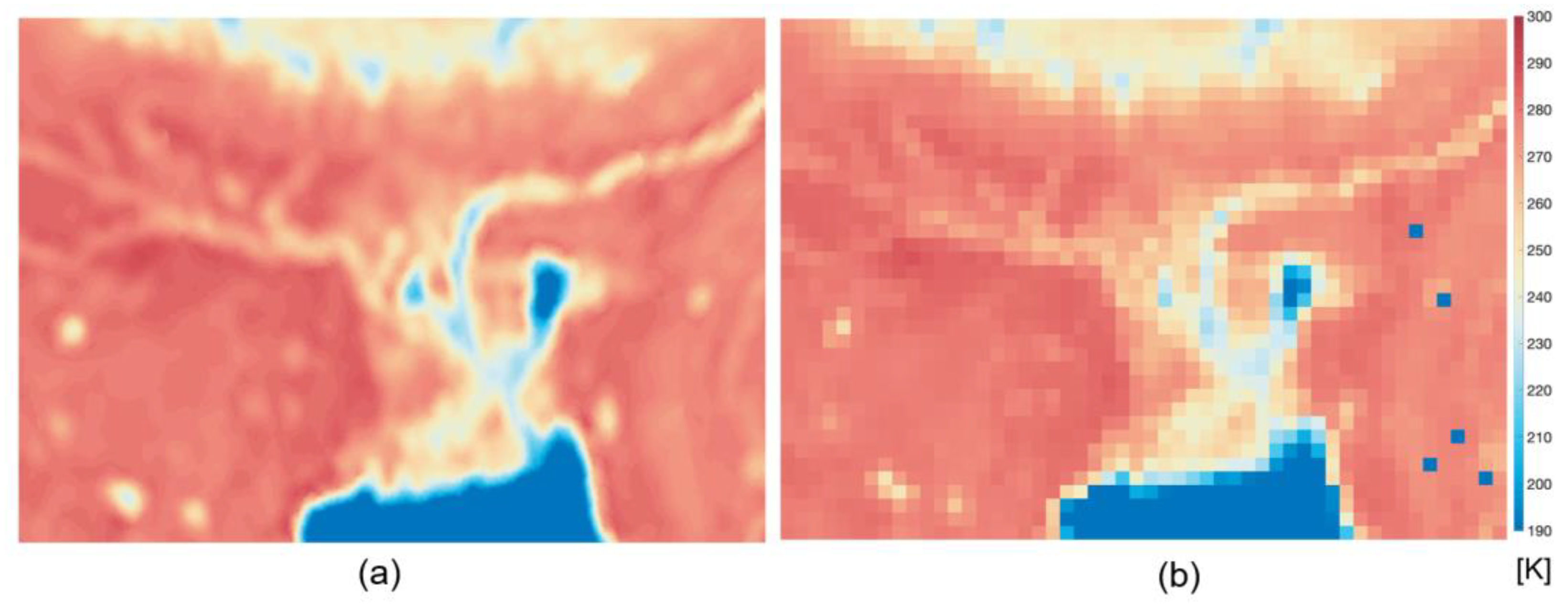
In this study, we make use of a spatially enhanced resolution product (named simply “enhanced” in the following), produced and distributed within the framework of a NASA MEASURES project [16]. The spatial enhancement is achieved through the application of a radiometer version of the Scatterometer Image Reconstruction technique (rSIR), gridding overlapping swath data by means of the effective measurement response function (MRF) together with the scan geometry and the integration period [19]. This technique represents a large improvement when compared with the more basic “drop-in-the-bucket” gridding method (based on a simple average of all the measurements falling into the pixel) historically used to generate the coarser resolution dataset. The final spatial resolution at which the enhanced product is generated is a function of the frequency. Data at 37 and 89 GHz are generated at a resolution of 3.125 km, 19 GHz at 6.125 km, and the remaining lower frequencies at 12.5 km. A consistent version of the product at a spatial resolution of 25 km is also produced and distributed (and it is also used in this study). More information about the spatially enhanced product is available at https://nsidc.org/data/nsidc-0630 (last access 21 February 2022). Here, we use the 37 GHz brightness temperature produced at 3.125 km because of the high spatial resolution and because it has been proven to be effective in mapping floods in other studies [5,6,7,10,12,13]. We excluded the 89 GHz (which has a similar spatial resolution of the 37 GHz) because of its strong sensitivity to atmospheric processes that would impact our estimates. We report results obtained using the horizontal polarization, as our analysis (not shown here) indicates that this polarization is most sensitive to flood events, in agreement with previous studies [5,7]. As an example, Figure 2 shows the map of brightness temperature at 37 GHz, horizontal polarization, ascending pass in the case of the enhanced (Figure 2a) and coarse (Figure 2b) resolution for data collected on 10 October 2005 over the study area during the flood event.

2.3. Passive Microwave Flood Detection Method

Approaches for detecting floods from PMW data build on the contrast between the emissivity of dry and flooded/wet surfaces. Typically, emissivity values for water are around 0.5, and for most minerals, values are between 0.75 and 0.95 [20]. Such contrast has allowed the development of techniques based on PMW data that, under the assumptions discussed below, allow us to estimate the presence of surface water within the observed scene. Beside intrinsic limitations of the different algorithms, we point out here that PMW data can be sensitive to soil moisture and heavy precipitation, depending on the frequency. In general, the lower the frequency, the higher the sensitivity to soil moisture and lower to precipitation. In this regard, the 37 GHz channel has been shown to provide optimal results [12] and, as we will see in the next section, is delivered at an unprecedented spatial resolution of 3.125 km through a new NASA product.
The method that we apply here is based on the work by De Groeve [5], who proposed an approach based on the assumption that geographically close pixels have similar land surface properties (i.e., temperature, roughness, vegetation, etc.). This approach relies on the selection of a calibration brightness temperature aimed to remove the effect of the surface temperature from the time series. In the method, the measured brightness temperature value of an area (Tb,m) is assumed to be expressed as the linear combination of water-covered (i.e., flooded, Tb,w) and dry brightness temperatures (Tb,d), weighted through fractional flooded area w as follows:
Tb,m = (1-w)Tb,d + wTb,w = Tm [(1−w) εd + wεw],
where εw and εd are the water and dry land emissivities, respectively, and Tm is the physical surface temperature of the area within the measurement pixel. In order to detect floods, brightness temperature values are normalized through a calibration brightness temperature Tb,c, defined as:
Tb,c = Tb,d = Tcεd,
where Tc is the physical surface temperature of the area within the calibration pixel. If for nearby pixels we assume,
εd,m ≈ εd,c ≈ εd and Tm ≈ Tc,
then we can define a signal S as the ratio between measurement (M) and calibration (C) brightness temperature signals:
S = M/C = Tb,m/Tb,c = {Tm [(1−w)εd + wεw]}/Tcεd ≈ 1 − w + w(εwd),
According to Equation (4), we can also express the water fraction within each pixel as follows:
w = (S − 1)/(εwd − 1),
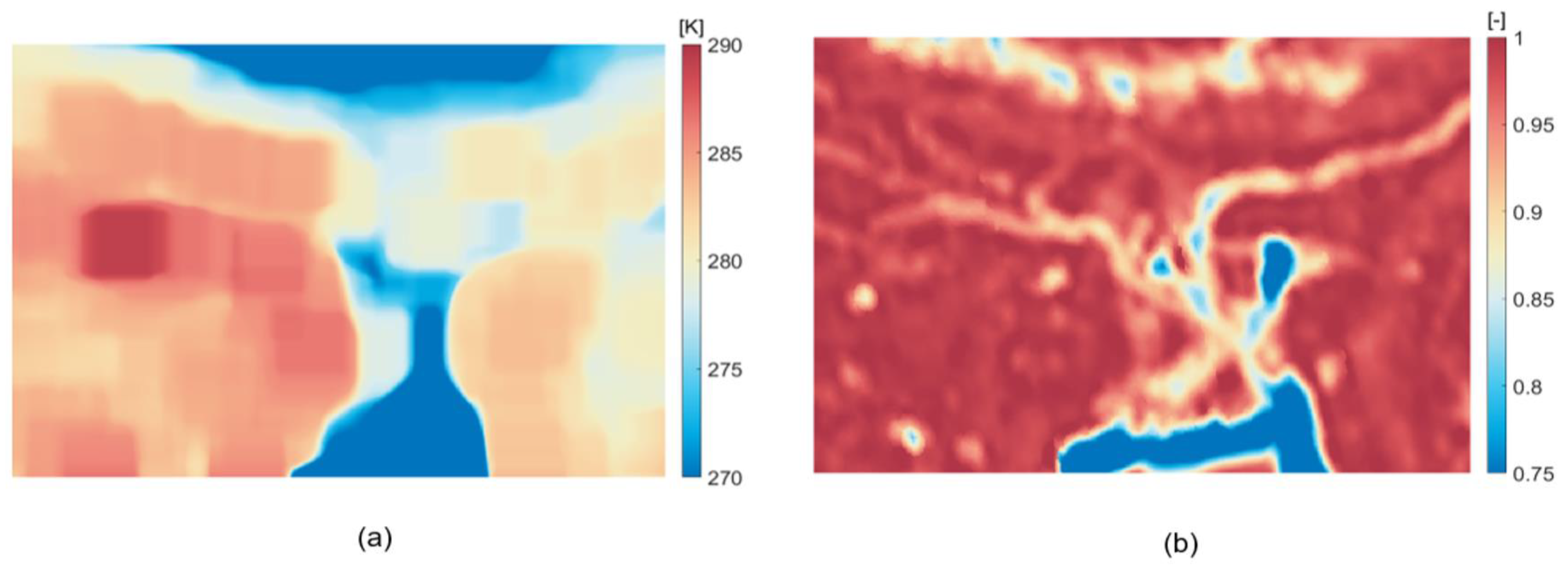
For each pixel, we compute the calibration brightness temperature automatically as the maximum brightness temperature value within a square area of 24 pixels centered at the specific pixel where flood is being monitored. The number of pixels was selected to match the original area size used in [5]. A pixel is flagged as flooded when S drops below a threshold value, computed as the 5th percentile of the time series (adopted here) or a fixed number of standard deviations from the mean, 2 in the case of regular floods and 4 in the case of large floods [5]. Figure 3 shows an example of the maps of the calibration (C, Figure 3a) and measured (M, Figure 3b) brightness temperatures over the test region of Bangladesh obtained from the enhanced resolution satellite image of 10 October 2005.

2.4. MODIS Data and the Normalized Difference Water Index

In order to assess the performances of the PMW algorithm, we collected Moderate Resolution Imaging Spectroradiometer (MODIS) reflectance data acquired by the TERRA and AQUA satellites over the area of interest [21]. Images were georeferenced and areas covered by clouds were removed using the internally provided quality flag. In order to map inundated areas, we use the Normalized Difference Water Index (NDWI, [21]), expressed as:
NDWI = (XNIR – XSWIR)/(XNIR + XSWIR),
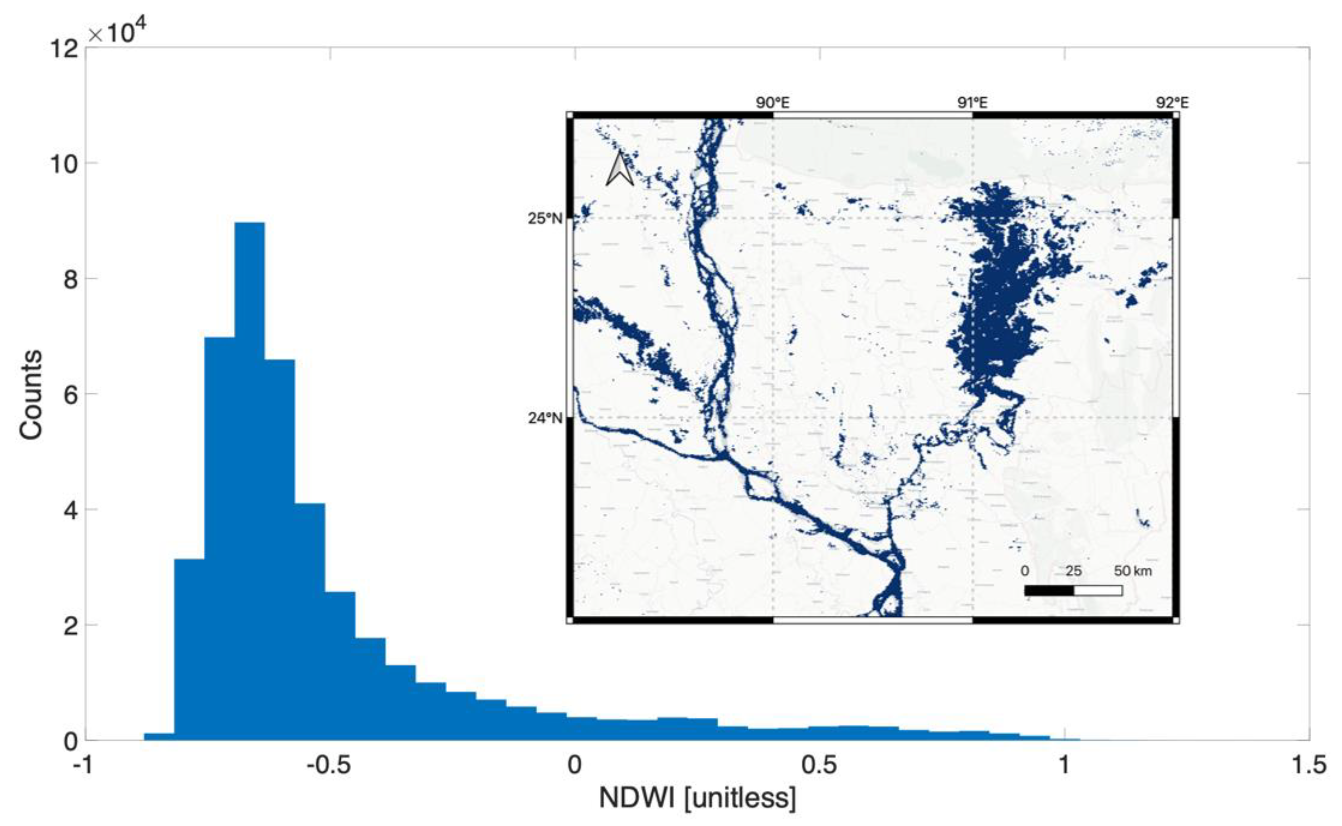
where XNIR and XSWIR are the near-infrared and short-wave infrared channels, respectively. Surface water is assumed to be present when NDWI exceeds the value of 0 [22]. As an example, Figure 4 shows the histogram of NDWI values computed from MODIS at the spatial resolution of 500 m for 10 October 2005.

2.5. Water Level Data

As a point-scale indicator of the flood event, we used water level data measured by the hydrometric stations distributed over the research area. Here, we chose to use the water level data in proximity of the selected pixels for the time series analysis. Specifically, we considered the Mohadebpur station, in the Naogaon district (station ID SW145), located at 24.9158 N and 88.7500 E (Figure 1). We considered the two-month interval centered in the proximity of the flood event (September and October 2005).

2.6. Spatial Scale analysis and Semi-Variograms

To further investigate the information content associated with the enhanced resolution of the PMW product with respect to the coarse one, we performed a semi-variogram analysis to study the spatial scales of the parameters used to characterize flooding (i.e., NDWI in the case of MODIS and the signal S in the case of the PMW datasets). A semi-variogram can be seen as a descriptor of the spatial continuity of the data, describing the spatial autocorrelation of the elements within the scene. We computed the empirical semi-variogram as:
γ(h) = (2N(h))−1Σ(i,j)∈N(h) (zi − zj)2,
where N(h) stands for the number of pair observations (i,j) separated by a spatial distance h [23]. The terms zi and zj are the attribute values of observations i and j, respectively. Generally, as the distance between observations increases, the semi-variance γ is likely to increase because near-observations are more likely to be spatially correlated. The semi-variance is then plotted as a function of the distance h to obtain the so-called experimental variogram. Lastly, this is fitted with a function to calculate the following three parameters characterizing the semi-variogram: the nugget, sill, and range. In this study, we used a spherical function [23] to fit the experimental variorum as it is the function that provided the best fitting among all considered functions. The nugget represents the small-scale spatial variations within the fields. This is an indicator of how noisy the spatial structure is. For instance, inside the fields, there exists some small-scale intrinsic variability, which accounts for the fact that not all neighbors can be exactly similar. The sill corresponds to the value when the semi-variances reach a plateau and stabilize. The range is the distance beyond which observations are no longer spatially correlated. Above the range distance, observations do not share any relationship, or complementarily, observations within the range are spatially correlated and share similar drivers and processes [24]. Such information can describe the spatial coherence of the dataset considered with respect to the reference dataset (i.e., MODIS).

2.7. AMSR-E Emissivity Data and Water Fraction Extraction

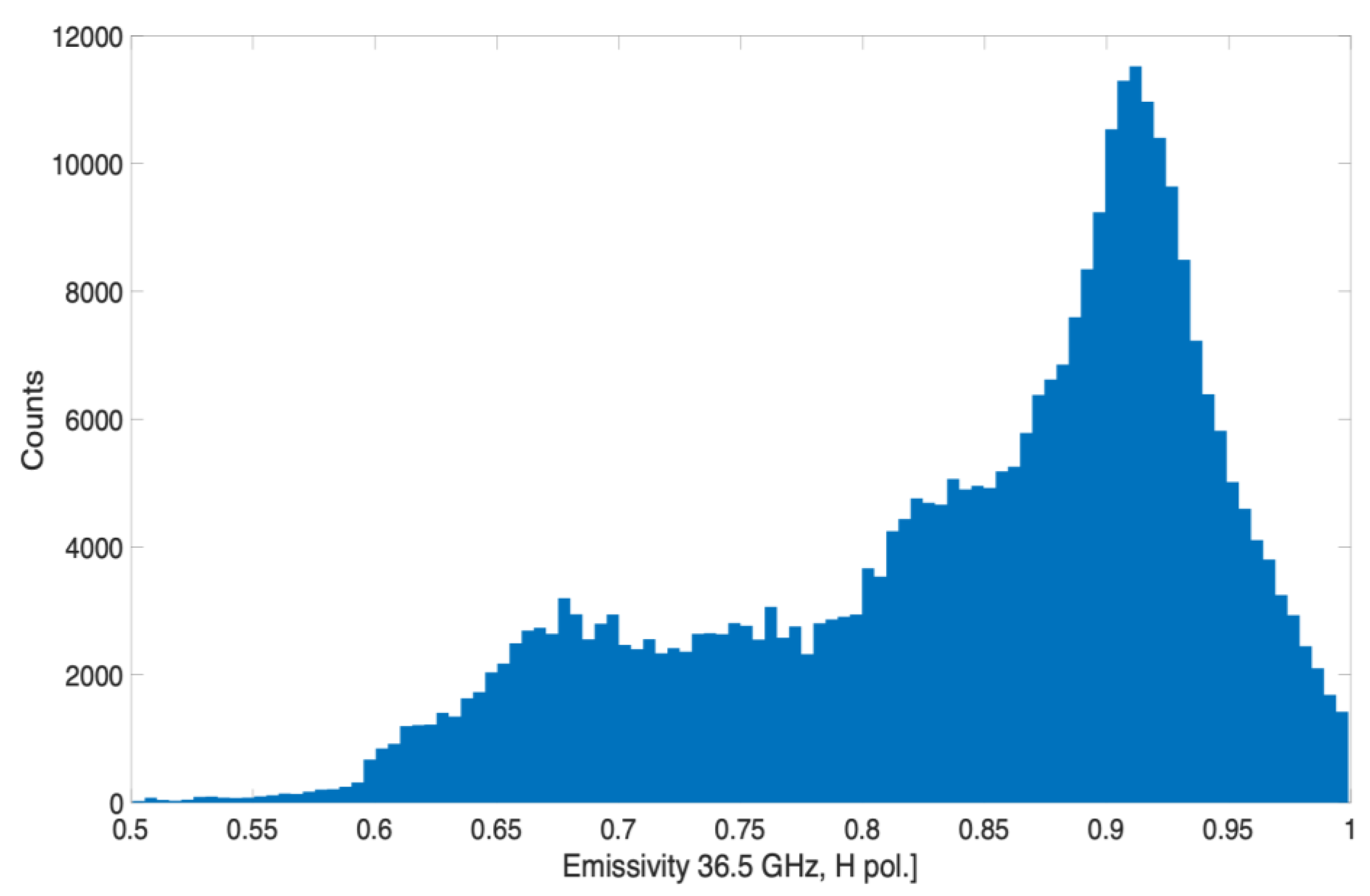
We also address the possibility of retrieving the fraction of the pixel covered by the flood, w in Equation (5) from the PMW data. In order to solve Equation (5) for w, we need to assign values to the water and land permittivity values (εwater and εland). As mentioned, the values can range greatly, and to assess optimal values for the inversion in our case, we make use of a dataset containing global land emissivity product obtained from PMW observations collected by the Advanced Microwave Scanning Radiometer—Earth Observing System (AMSR-E, [25]). As an example, we show the histogram of the monthly emissivity values estimated at 36.5 GHz over our area of interest for the month of October 2005 (Figure 5) when the flood occurred. From the histogram, we assume the emissivity in the case of dry pixels to be the peak value of the histogram (0.93) and the emissivity value in the case of flooded areas to be the 5th percentile of the values (0.58). After selecting these values, we visually inspected the emissivity map to verify that pixels presenting such values (0.93 or 0.58) were indeed located over flooded areas or water bodies. We realize there is room for refinement of these assumptions and improvement of the way the emissivity can be estimated, but our goal in this study is to provide a first analysis on the potential of the PMW dataset to extract fractional flooded areas. In order to evaluate the goodness of such an estimation of water fraction obtained from the PMW datasets, we compare it with the estimate obtained by resampling the 500 m MODIS flood maps at the 3.125 km and 25 km spatial resolutions.

3. Results and Discussion

3.1. Spatial Coverage

Because of the novelty of the product and of the new resampling adopted for generating the enhanced product, we first assessed the coverage of the spatially enhanced product over our study area. This is important in view of the benefits arising from the large swath associated with PMW sensors and the possibility of reaching a high temporal resolution for a near-real-time monitoring of floods. Our results indicate that the coverage of each sensor considered separately reaches relatively low values (~20% of the total area) because of the design orbit of the PMW spaceborne sensors, which reduces coverage at lower latitudes. Nevertheless, the fractional coverage increases considerably (average 97.8%) when considering all sensors. Moreover, the mean coverage increases to 99.7% when combining ascending and descending passes, with minimum values exceeding 95%. Such results indicate that the PMW-enhanced dataset is a reliable tool in terms of spatial and temporal coverage, providing useful data over the area of interest at high temporal resolution even in the enhanced case.

3.2. Time series Analysis

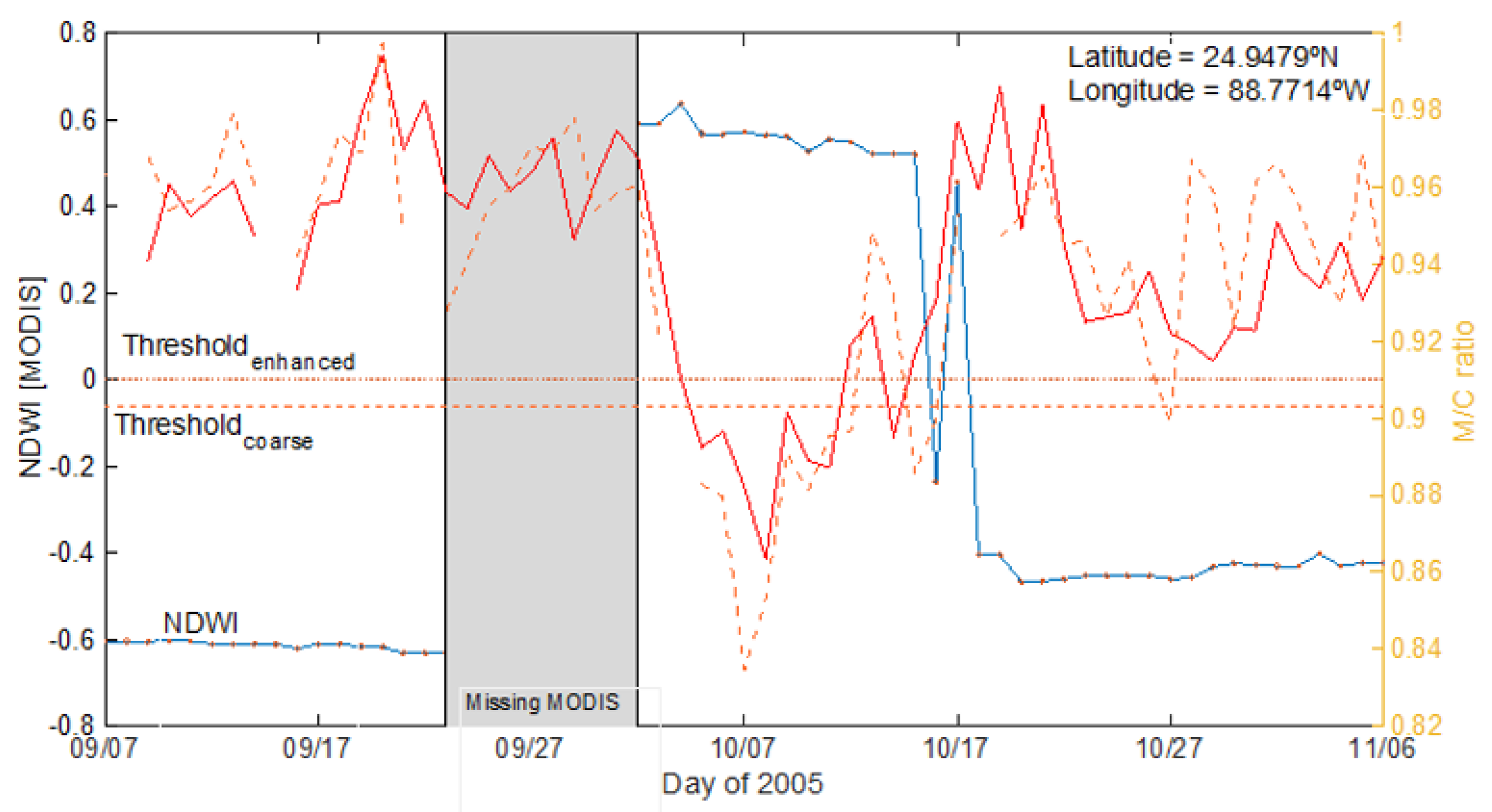
As a first step, we perform a comparison of time series of NDWI and the microwave signal S over different regions to better understand the linkages and relationships between the optical and the PMW datasets used for the flood detection. At this stage, we focus on a single gauged area strongly inundated in October 2005 to evaluate the temporal evolution of the flood event. The event was selected because of the availability of optical data that can be used as a validation dataset and because the flood was extensive enough to be captured by the relatively coarser spatial resolution of the PMW datasets. Specifically, in Figure 6, we show the time series of NDWI MODIS (blue, left y-axis) and of the signal S in the case of enhanced (red line, right y-axis) and coarse (dashed red line, right y-axis) for a location near the Mohadebpur station, where a major flood event was recorded at the beginning of October. We selected the coordinates (24.9479° N, 88.7714° W) for the plotted data based on the condition that flooding would be present in and on the availability of cloud-free MODIS images during that period. Threshold values computed for the PMW signals in the case of either the enhanced or the coarse PMW products are reported in the figure as dotted (enhanced) and dashed (coarse) horizontal lines.
From Figure 6, we note that on 3 October 2005, the day of the first available MODIS cloud-free data after the flood began for this specific location, both coarse and enhanced PMW signals begin to decrease as a consequence of the presence of flooded areas within the area covered by each pixel, then increase again and reach pre-flood values on 17 October 2005, a day before NDWI values become negative (pointing to the absence of flooded areas). We also note that the coarse resolution product suggests flooding on 27 October 2005, where both the enhanced product and MODIS do not. In this case, we note that the signal barely exceeds the selected threshold, and the missing of the flood detection is intrinsically related to the sensitivity of the algorithm and the threshold selection. With this in mind, this single-day event could be, eventually, filtered in a post-processing phase using multi-temporal analysis or considering a range of thresholds with which to build a composite or an ensemble of outputs that could define the probability of flooding to be occurring from PMW data. Such analysis confirms the strong dependence of the PMW signal on the presence of water on the observed surface.
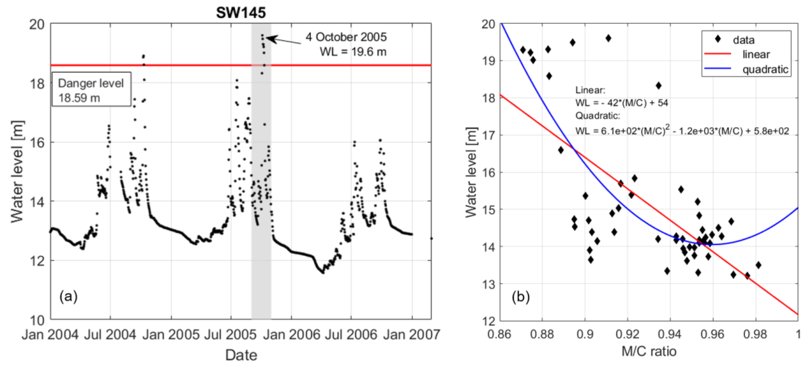
The comparison with MODIS data presented in Figure 6 exploits the coherence of the PMW signal with optical observations and highlights the limitation of optical data in case of cloud cover. However, a comparison with ground observations is needed to evaluate the capability of PMW sensors in capturing the hydrologic response to the flood event. By looking at the measured water level data at the Mohadebpur station, we evaluated the sensitivity of the M/C ratio to the flood event evolution. For this purpose, we considered the period September–October 2005, temporally embracing the flood event that occurred at the beginning of October. In Figure 7a, we show the water level measured for the period January 2004–February 2007. The gray shaded area indicates our period of interest. From the station time series, we see that the flood event we selected for this study shows the highest water level over the three-year period, overcoming the danger level (i.e., the water level at which the government expect damages in the nearby area) for seven consecutive days after 4 October 2005. In Figure 7b, we present the scatter plot obtained by comparing the measured water level at Mohadebpur station and the M/C ratio obtained from the enhanced resolution pixel reported in Figure 6, for the September–October period. Linear and quadratic regressions show, as expected, the decreasing relationship between the two considered variables. These results, similarly to what has been found in [5,7], point to the capability of the PMW signal to follow the hydrologic evolution of the flood event, capturing both low and high flow phases, with the quadratic model better fitting the data points (R2 = 0.51) than the linear model (R2 = 0.43). A similar relationship has been found in [10], where the fractional flooded area has been linked with the M/C signal.

3.3. Commission, Omission, and Matching Analysis

We compute the matching, omission, and commission errors between the results obtained with the PMW and MODIS over the Intensive Study Area as follows. Matching is calculated as the percentage of pixels that were correctly classified as flooded by the PMW product with respect to those obtained from MODIS; omission is defined as the percentage of the number of pixels that are classified as flooded from MODIS but not by the PMW product (complementary to matching); and lastly, commission error is estimated as the percentage of the pixels classified as flooded by the microwave product but not by the reference dataset. The results of these errors integrated over the Intensive Study Area are reported in Figure 8 as a function of the water fraction, computed as the fraction of the area within each PMW pixel (e.g., 3.125 km or 25 km) covered by water according to the MODIS analysis and fixed as the threshold for the analysis. In other words, the matching, commission, and omission errors are computed over the area presenting a flooded fractional area larger than the threshold value reported on the x-axis in Figure 8. In the table, we show the results for both enhanced and coarse resolution products when comparing data from the same day when flooding is detected and when flooding occurs for 3 days in a row for all sensors. We performed this analysis to study the sensitivity of the results of the PMW-based approach to the persistency of the flood.
The results in Figure 8 indicate that, overall, the commission error is not as sensitive as the matching to the water fraction, suggesting that the commission error might be related to intrinsic limitations of the PMW algorithm. This is likely because the PMW algorithm was not developed to directly map flood extent but rather to estimate the probability of a pixel to be flooded. Moreover, differently from the NDWI, PMW data can be sensitive to soil moisture and heavy precipitation, suggesting the presence of flooded regions where it might not actually be occurring and leading to over prediction. Lastly, the relatively larger pixel size (of either the gridded product and the original instantaneous field of view of the sensor) might be integrating information content from the regions surrounding the area where the comparison between the optical and PMW data is performed, hence introducing potential biases and differences. In this regard, the relatively high values of matching between the reference dataset and the results obtained with the spatially enhanced dataset results are encouraging, as they highlight the potential of the enhanced product for detecting floods with improved accuracy compared to previous microwave products. These results point out the limitations of using PMW data as a standalone product. A possible way to control the problems of overestimation/underestimation linked to the sensitivity to surrounding areas is to adopt a data fusion methodology, possibly using high-resolution data (e.g., optical and/or radar) together with topographical and hydrographical information (e.g., digital elevation model and river network).
The matching (M) systematically increases in all cases as the water fraction increases. This is not unexpected, as the larger the area covered by the flood, the stronger is the integrated effect on the brightness temperatures. Maximum values for the matching are reached in the case of the enhanced product for the flooded fraction area ranging between 0.9 and 1, showing best performances in areas strongly inundated or of permanent surface water. The commission error (C) in the case of the enhanced product is the lowest, ranging from 17.3% in the case of the 0–0.1 flood fraction to 9.8% in the case of the 0.9–1 flooded fraction area range. The enhanced product outperforms (both in terms of matching and commission error) the coarser product, with the matching in the case of the coarse product being lower than in the case of the enhanced product by 20–40% (e.g., relative change in the case of the coarse product with respect to the results obtained in the case of the enhanced product). The commission error also reaches relatively high values in the case of the coarse product, peaking to 32.2% and averaging 23.8% (1 day) and 24.7% (3 days) versus average values in the case of the enhanced product of 14.7% (1 day) and 15.1% (3 days). The commission error does not show sensitivity to the flooded fractional area, suggesting a possible intrinsic bias of the PMW data, in agreement with the results found in [5]. Another issue might be related to soil moisture, slightly affecting the 37 GHz, as described in [13]. A hydrological soil model including evapotranspiration in combination with a soil emission model could better quantify this issue. The scores computed in the case of 0 flood fraction confirm the limitations in using the PMW product over the whole study area, suggesting the possibility to limit the application in the nearest area to the surface water bodies.
The results of the comparison between PMW and optical data are also impacted by the different spatial scales at which the different sensors “see” the scene under observation. In order to partially investigate this aspect, we degraded the original MODIS data from the spatial resolution of 500 m to the 3.125 km and 25 km spatial resolution and computed the flooded area using the spatially degraded products. Our results are summarized in Figure 9, showing two examples of NDWI maps for 10 October (a,c,e) and 24 October (b,d,f) obtained from MODIS data at the original 500 m spatial resolution (a,b), at 3.125 km (c,d) and 25 km (e,f). The results obtained for the two dates are consistent and indicate that the flooded area estimated through the NDWI decreases by ~20% (with respect to the original 500 m MODIS resolution) when degrading the resolution from 500 m to 3.125 km and by a further ~10% when degrading it to 25 km. The results shown in Figure 9 suggest that a systematic bias of ~20% in the case of the enhanced product and ~30% in the case of the coarse product might need to be considered because of the differences in the spatial resolution of the original datasets.

3.4. Spatial Autocorrelation Analysis

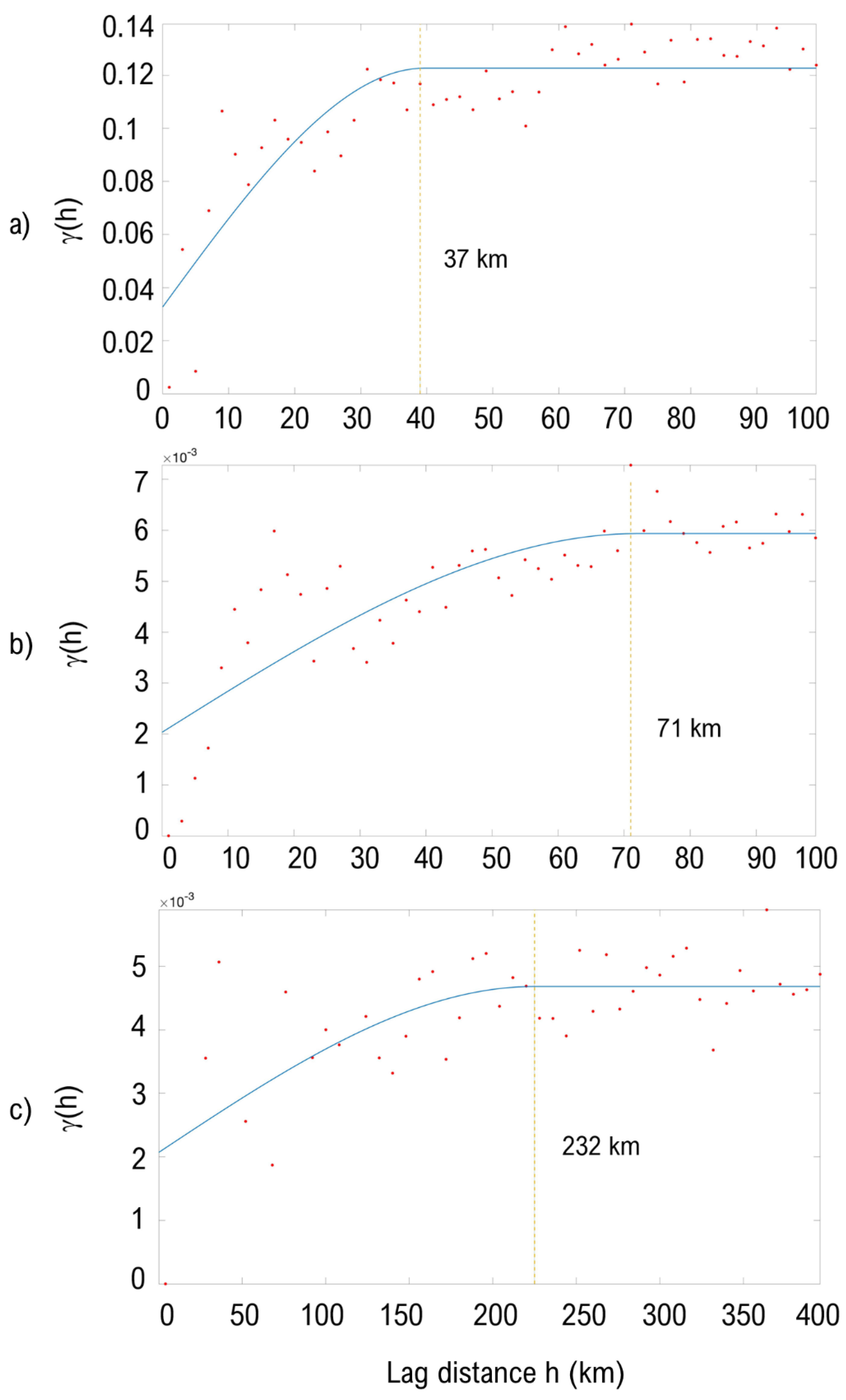
To investigate the information content of the enhanced product, we performed a spatial autocorrelation analysis following the approach proposed in [17], where a similar analysis is also performed on the enhanced PMW product. Examples of semi-variograms computed for the NDWI and the signal S in the case of the enhanced and coarse PMW data for 10 October 2005 over the Intensive Study Area are reported in Figure 10. The semi-variogram in the case of the NDWI dataset (Figure 10a) indicates that NDWI data have a range of ~37 km (meaning that the NDWI values within that distance are spatially autocorrelated and suggesting that, similarly, the processes driving the variability for NDWI are occurring below that spatial scale). On the other hand, the range computed in the case of the enhanced product is ~71 km (Figure 10b), against a value of 232 km (Figure 10c) in the case of the coarse product. The value of the spatial autocorrelation length in the case of the enhanced product indicates that it is more sensitive to the processes driving the spatial variability of the flood than the coarser product, highlighting the benefits associated with the enhanced product.

3.5. Water Fraction Estimation

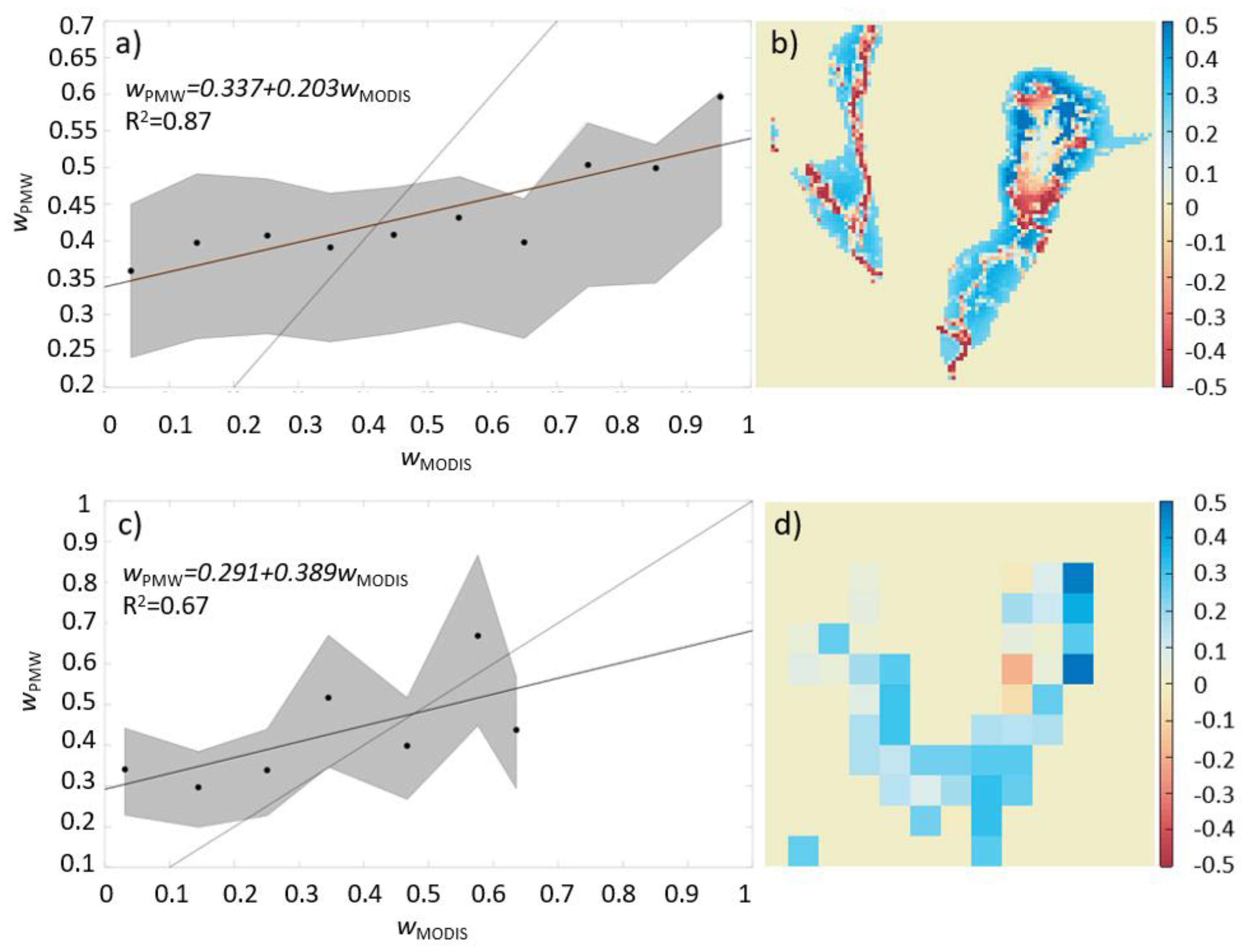
Lastly, we performed the estimate of water fraction (w) according to Equation (5), obtaining the estimates of permittivity values for land (εw) and water (εd) from the AMSR-E surface permittivity dataset, in the case of both the enhanced and coarse products. We evaluate such an estimate by comparing the spatial distribution of the fractional flooded area within each pixel with that obtained from the 500 m MODIS binary when resampling it to the 3.125 and 25 km spatial resolutions. In the case of the MODIS degraded products, each pixel contains the percentage of pixels classified as flooded with respect to the total number of the 500 m pixels falling within the 3.125 km (or 25 km) pixel. The maps of the differences between the fraction of flooded area estimated from the two PMW products and from the optical data are reported in Figure 11b (enhanced) and 11d (coarse). In general, both products tend to overestimate the fraction of flooded area estimated through MODIS. However, the enhanced product is capable of providing more details of the spatial distribution of the flood, with a mean error of −0.04 and a standard deviation of 0.28 (vs. a mean of −0.12 and a standard deviation of 0.38 of the coarse product). The enhanced product underestimates flood extent, for example, along major rivers. This might be due to the “spilling” effect of the pixels surrounding those containing the river which, in turn, occupies only a relatively small fraction of the 3.125 km (or 25 km) pixel. On the other hand, the overestimation of the fraction of flooded area by the PMW as one moves away from the river might be due to the sensitivity of the PMW to soil moisture that is, however, not detectable by optical data. A comparison with water level measurements and modeled inundation maps might shed light on this in future research, together with extending this analysis to other dates.
We also investigated the relationship between the fraction of flooded area derived from MODIS and from the PMW products through a linear regression analysis. To reduce the noise of the datasets, we grouped the values of the mapped fraction of flooded area into 10 bins ranging between 0 and 1 (step 0.1) in which the value of the fraction was obtained from the average within that range of the mapped values. Figure 11a,c show the fraction of flooded area estimated from the enhanced (Figure 10a) and coarse (Figure 11c) products as a function of the one estimated from MODIS. As noticed, the PMW products tend to overestimate the values obtained with MODIS (as discussed above concerning soil moisture), but there is a promising relationship between the two datasets that suggests the possibility of using the microwave products after refinements (e.g., improvements in terms of data aggregation from different sensors or signal smoothing). To investigate the sensitivity of the PMW retrieval to the choice of the permittivity values, we also computed the values of fractional area using two sets of values for the water and land permittivity of (0.95, 0.5) and (0.9, 0.6). The estimated values are the lines bonding the gray area in Figure 11a,c. This analysis confirms the strong information content of the PMW data to the percentage of the sensed area covered by water, similarly to the results obtained in [10], where a quadratic relationship between M/C ratio and surface water fraction was found. Certainly, such a simple evaluation of the fractional flooded area cannot be used as an indicator for operational applications or directly applied for flood index insurance. This method has been designed and previously applied to the 25 km resolution PMW dataset to monitor large-scale flood events [5] where a minimum flood extent of 1000 km2 was detected. In [10], a quadratic relationship between fractional flood extent and M/C signal was found, with minimum water fraction captured by the M/C signal of about 0.1%, suggesting a decreasing sensitivity for decreasing water fraction. This aspect is also suggested by the intercept of the linear regression curve obtained, with a PMW-derived water fraction showing an overestimation for small MODIS-derived water fraction values. The commission, omission, and matching analyses confirm this issue. However, the sensitivity to the presence of water of the PMW sensors in general and the improved spatial representation introduced by the enhanced resolution dataset open the door to the development of downscaling algorithms.

4. Conclusions

We investigated the application of spatially enhanced spaceborne PMW brightness temperatures to map a flood over an area in Bangladesh that occurred in October 2005. We compared maps of flooded areas obtained with the enhanced product with those obtained from the coarse (i.e., 25 km) PMW product and from optical data collected by the MODIS sensor at a spatial resolution of 500 m. As one of the major advantages of using PMW data is the high temporal frequency and spatial coverage, and given the novel nature of the enhanced product used here, we first estimated the percentage of our study area that was covered by the enhanced PMW data on a daily basis. We found that, when considering all sensors and orbits (e.g., ascending and descending), the coverage of the area interest exceeds 99% on a daily basis. This aspect is important as it offers the possibility of using such a dataset for operational purposes (e.g., near-real-time monitoring, insurance applications, etc.). The comparison between the extent of the flood obtained with the enhanced and the coarse products indicates that the noise introduced by the spatial enhancement (e.g., [16]) does not appear to be a limit for the application of the product to flood mapping with respect to the coarser product.
Overall, we found that flood mapping derived from the enhanced resolution PMW better agrees with the one obtained from MODIS than the one obtained with coarse resolution data. One aspect that we investigated is the sensitivity of the results to the spatial resolution. We found that the enhanced product appears to be more sensitive to the presence of a flood than the coarse one and we suggest this is due to the improved spatial resolution which allows better separation of dry from wet regions. Overall, the best results were obtained when the relative fraction of flooded area within each PMW pixel was high (e.g., >0.9), with the matching between the optical and PMW data degrading as the fraction of flooded area decreases. This is not unexpected, given the nature of the PMW data which “integrates” the effects of the features within each pixel and, therefore, becomes less and less sensitive to floods as the fraction of flooded area decreases. However, high commission errors for low values of water fraction were found, indicating over prediction in some areas where the soil might be just a little moist.
On spatial resolution and information content, we also investigated the spatial autocorrelation of the three datasets (two PMW and one optical) through a semi-variogram analysis. We found that, also in this case, the spatially enhanced product outperforms the coarse product, as the scale breaks in the case of the enhanced product are much closer to those obtained with MODIS. This complements the results obtained in terms of matching, discussed above, and indicates that the enhanced product is more coherent with the higher-resolution MODIS dataset in capturing flooding than the coarser product.
Lastly, our estimate of water fraction obtained using PMW data and AMSR-E permittivity to solve Equation (5) confirms the strong information content of PMW data, opening the possibility for future developments and operational applications. In conclusion, our analysis shows the capability of the enhanced resolution dataset to detect large-scale flood events. The error analysis confirms that the improvements in terms of spatial resolution of the historical dataset led to improvements in terms of flood detection sensitivity. Moreover, the variogram analysis confirmed the better representation of the spatial scale by the enhanced product with respect to the coarse one.
Given the capability of the PMW sensors to collect data in all weather conditions and, consequently, the availability of a long time series of daily maps, the PMW dataset can be considered a potential input to a machine learning algorithm. A combination of PMW imagery, higher resolution remote sensing data (e.g., MODIS and/or Sentinel), and topographic and hydrographic information (such as distance from rivers, distance from the coast, slope, etc.) can be used as an ensemble of features for training and testing a supervised algorithm using, for example, the high-resolution flood dataset published by Bonfilia et al. (2020) [26]. Considering the possibility of having a daily and continuous acquisition of the PMW data, there is potential for developing a high-resolution, near-real-time flood mapping system to be provided to decision makers or insurance companies, as proposed in [5], improving the current PMW tools [27] in terms of spatial resolution. Moreover, considering the long-term coverage of the PMW dataset (since 1979), it would be possible to create a historical flood map dataset, opening the possibility to build a stronger knowledge of the flood event return period, not only in terms of precipitation or stage level but also in terms of actual inundated areas.

Author Contributions

Conceptualization, P.C. and M.T.; Data curation, P.C., M.T. and E.T.; Funding acquisition, M.T. and E.T.; Investigation, P.C. and M.T.; Methodology, E.T.; Supervision, E.T.; Writing—original draft, P.C. and M.T.; Writing—review and editing, P.C., M.T. and E.T. All authors have read and agreed to the published version of the manuscript.

Funding

This study was funded by Cloud2Street LLC and by Columbia University (UR005706-BM).

Institutional Review Board Statement

Not applicable.

Data Availability Statement

Passive microwave data are available online at https://nsidc.org/data/nsidc-0630/versions/1 (last access 21 February 2022). MODIS data can be found at https://modis.gsfc.nasa.gov/data/dataprod/mod09.php (last access 21 February 2022). Processed data are available upon request to the corresponding author.

Acknowledgments

This research was supported by the Columbia World Project: ACToday at Columbia University in the city of New York. The authors would also like to thank Cloud2Street LLC for the support.

Conflicts of Interest

Authors declare no conflict of interest.

References

  1. Boni, G.; Ferraris, L.; Pulvirenti, L.; Squicciarino, G.; Pierdicca, N.; Candela, L.; Pisani, A.R.; Zoffoli, S.; Onori, R.; Proietti, C.; et al. A Prototype System for Flood Monitoring Based on Flood Forecast Combined With COSMO-SkyMed and Sentinel-1 Data. IEEE J. Sel. Top. Appl. Earth Obs. Remote Sens. 2016, 9, 2794–2805. [Google Scholar] [CrossRef]
  2. Twele, A.; Cao, W.; Plank, S.; Martinis, S. Sentinel-1-based flood mapping: A fully automated processing chain. Int. J. Remote Sens. 2016, 37, 2990–3004. [Google Scholar] [CrossRef]
  3. Amitrano, D.; Martino, G.D.; Iodice, A.; Riccio, D.; Ruello, G. Unsupervised Rapid Flood Mapping Using Sentinel-1 GRD SAR Images. IEEE Trans. Geosci. Remote Sens. 2018, 56, 3290–3299. [Google Scholar] [CrossRef]
  4. Ulaby, F.T.; Moore, R.K.; Fung, A.K. Microwave Remote Sensing: Active and Passive—3: From Theory to Applications; Artech House: Dedham, MA, USA, 1986. [Google Scholar]
  5. Groeve, T.D. Flood monitoring and mapping using passive microwave remote sensing in Namibia. Geomat. Nat. Hazards Risk 2010, 1, 19–35. [Google Scholar] [CrossRef]
  6. Sippel, S.J.; Hamilton, S.K.; Melack, J.M.; Choudhury, B.J. Determination of inundation area in the Amazon River floodplain using the SMMR 37 GHz polarization difference. Remote Sens. Environ. 1994, 48, 70–76. [Google Scholar] [CrossRef]
  7. Galantowicz, J. High-resolution flood mapping from low-resolution passive microwave data. IEEE Int. Geosci. Remote Sens. Symp. 2002, 3, 1499–1502. [Google Scholar]
  8. Schroeder, R.; Mcdonald, K.; Chapman, B.; Jensen, K.; Podest, E.; Tessler, Z.; Bohn, T.; Zimmermann, R. Development and Evaluation of a Multi-Year Fractional Surface Water Data Set Derived from Active/Passive Microwave Remote Sensing Data. Remote Sens. 2015, 7, 16688–16732. [Google Scholar] [CrossRef] [Green Version]
  9. Du, J.; Kimball, J.S.; Galantowicz, J.; Kim, S.-B.; Chan, S.K.; Reichle, R.; Jones, L.A.; Watts, J.D. Assessing global surface water inundation dynamics using combined satellite information from SMAP, AMSR2 and Landsat. Remote Sens. Environ. 2018, 213, 1–17. [Google Scholar] [CrossRef] [PubMed]
  10. Zeng, Z.; Gan, Y.; Kettner, A.J.; Yang, Q.; Zeng, C.; Brakenridge, G.R.; Hong, Y. Towards high resolution flood monitoring: An integrated methodology using passive microwave brightness temperatures and Sentinel synthetic aperture radar imagery. J. Hydrol. 2020, 582, 124377. [Google Scholar] [CrossRef]
  11. Allison, L.J.; Schmugge, T.J.; Byrne, G. A hydrological analysis of East Australian floods using Nimbus-5 electrically scanning radiometer data. Bull. Am. Meteorol. Soc. 1979, 60, 1414–1427. [Google Scholar] [CrossRef] [Green Version]
  12. Giddings, L.; Choudhury, B. Observation of hydrological features with Nimbus-7 37 GHz data, applied to South America. Int. J. Remote Sens. 1989, 10, 1673–1686. [Google Scholar] [CrossRef]
  13. Choudhury, B.J. Monitoring global land surface using Nimbus-7 37 GHz data theory and examples. Int. J. Remote Sens. 1989, 10, 1579–1605. [Google Scholar] [CrossRef]
  14. Prigent, C.; Matthews, E.; Aires, F.; Rossow, W.B. Remote sensing of global wetland dynamics with multiple satellite data sets. Geophys. Res. Lett. 2001, 28, 4631–4634. [Google Scholar] [CrossRef] [Green Version]
  15. Fluet-Chouinard, E.; Lehner, B.; Rebelo, L.-M.; Papa, F.; Hamilton, S.K. Development of a global inundation map at high spatial resolution from topographic downscaling of coarse-scale remote sensing data. Remote Sens. Environ. 2015, 158, 348–361. [Google Scholar] [CrossRef]
  16. Brodzik, M.J.; Long, D.G.; Hardman, M.A.; Paget, A.; Armstrong, R.L. MEaSUREs Calibrated Enhanced-Resolution Passive Microwave Daily EASE-Grid 2.0 Brightness Temperature ESDR, Version 1; Digital Media; National Snow and Ice Data Center: Boulder, CO, USA, 2018. [Google Scholar] [CrossRef]
  17. Colosio, P.; Tedesco, M.; Ranzi, R.; Fettweis, X. Surface melting over the Greenland ice sheet derived from enhanced resolution passive microwave brightness temperatures (1979–2019). Cryosphere 2020, 15, 2623–2646. [Google Scholar] [CrossRef]
  18. Chowdhury, M.R.; Ward, N. Hydro-meteorological variability in the greater Ganges-Brahmaputra-Meghna basins. Int. J. Climatol. 2004, 24, 1495–1508. [Google Scholar] [CrossRef]
  19. Williams, B.A.; Long, D.G. Reconstruction from Aperture-Filtered Samples with Application to Scatterometer Image Reconstruction. IEEE Trans. Geosci. Remote Sens. 2011, 49, 1663–1676. [Google Scholar] [CrossRef] [Green Version]
  20. Rees, W.G. Physical Principles of Remote Sensing; Cambridge University Press: Cambridge, UK, 1990. [Google Scholar]
  21. MODIS Web. Available online: https://modis.gsfc.nasa.gov/data/dataprod/mod09.php (accessed on 17 January 2022).
  22. Gao, B.-C. NDWI—A normalized difference water index for remote sensing of vegetation liquid water from space. Remote Sens. Environ. 1996, 58, 257–266. [Google Scholar] [CrossRef]
  23. Webster, R.; Oliver, M.A. Geostatistics for Environmental Scientists; John Wiley & Sons: New York, NY, USA, 2001. [Google Scholar]
  24. Deems, J.S.; Fassnacht, S.R.; Elder, K.J. Fractal Distribution of Snow Depth from Lidar Data. J. Hydrometeorol. 2006, 7, 285–297. [Google Scholar] [CrossRef]
  25. Norouzi, H.; Temimi, M.; Rossow, W.B.; Pearl, C.; Azarderakhsh, M.; Khanbilvardi, R. The sensitivity of land emissivity estimates from AMSR-E at C and X bands to surface properties. Hydrol. Earth System Sci. 2011, 15, 3577–3589. [Google Scholar] [CrossRef] [Green Version]
  26. Bonafilia, D.; Tellman, B.; Anderson, T.; Issenberg, E. Sen1Floods11: A georeferenced dataset to train and test deep learning flood algorithms for Sentinel-1. In Proceedings of the IEEE/CVF Conference on Computer Vision and Pattern Recognition Workshops, Seattle, WA, USA, 14–19 June 2020; pp. 210–211. [Google Scholar]
  27. Jensen, K.; Mcdonald, K. Surface water microwave product series Version 3: A near-real time and 25-year historical global inundated area fraction time series from active and passive microwave remote sensing. IEEE Geosci. Remote Sens. Lett. 2019, 16, 1402–1406. [Google Scholar] [CrossRef]
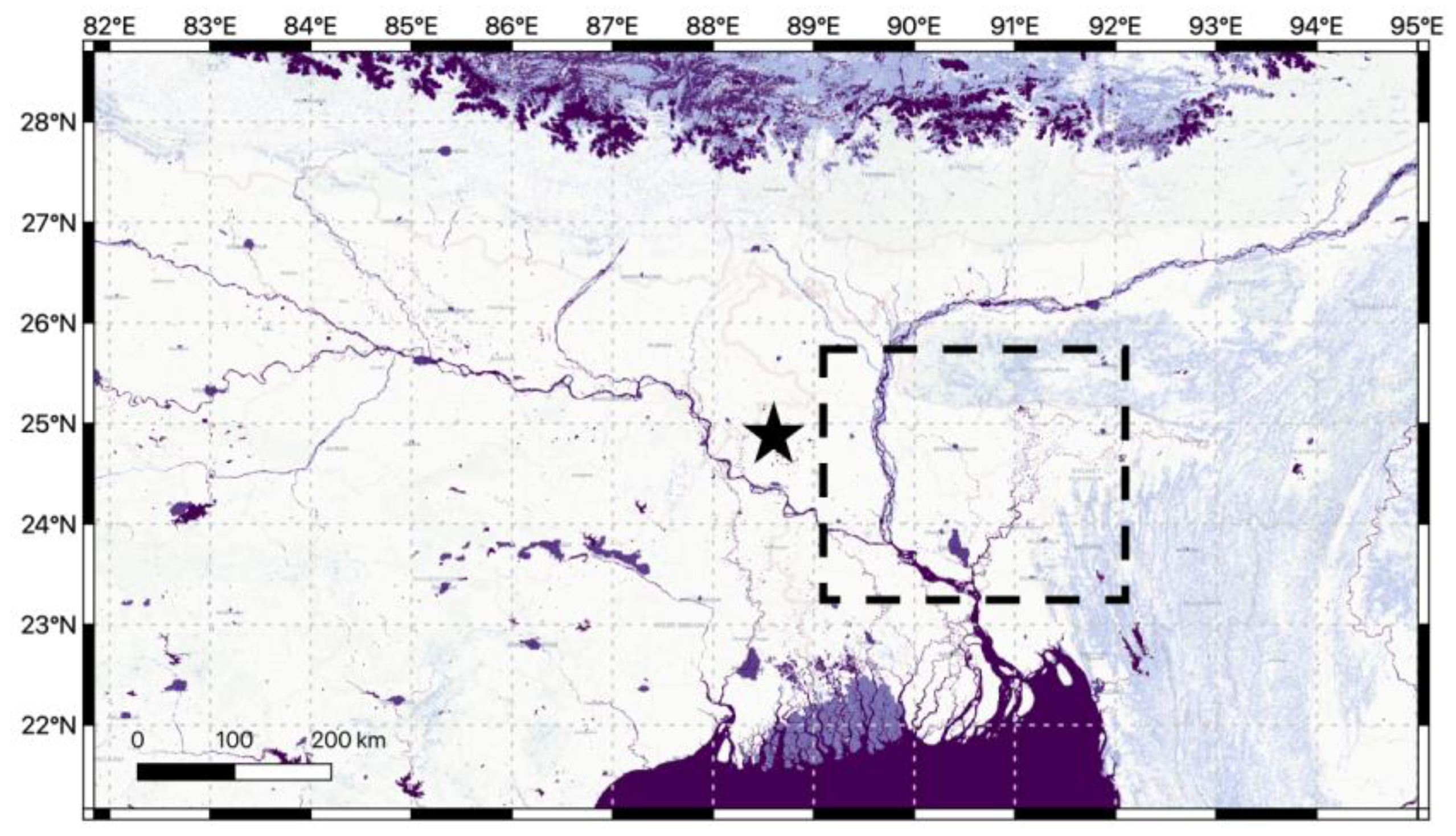
Figure 1. Original study area considered in this study. Shades of blue show the presence of water bodies as obtained from the MODIS land use/land cover (LULC) product (https://lpdaac.usgs.gov/products/mcd12q1v006/, last accesses 21 February 2022). The dashed-line rectangle shows the location of our Intensive Study Area (ISA). The black star represents the location of the hydrometric station considered.
Remotesensing 14 01180 g001
Figure 2. Maps of (a) spatially enhanced and (b) coarse brightness temperatures at 37 GHz, ascending pass, horizontal polarization collected over the study area on 10 October 2005 (day of the year 281).
Remotesensing 14 01180 g002
Figure 3. Example of maps of (a) calibration C brightness temperature and (b) signal S over the study area (10 October 2005).
Remotesensing 14 01180 g003
Figure 4. Histogram of NDWI values computed from MODIS at the spatial resolution of 500 m for 10 October 2005. The inset shows the distribution of water bodies on the surface as detected when assuming NDWI > 0.
Remotesensing 14 01180 g004
Figure 5. Histogram of emissivity values for the month of October 2005 at 36.5 GHz, horizontal polarization, obtained from AMSR-E over the study area.
Remotesensing 14 01180 g005
Figure 6. Time series of NDWI MODIS (blue, left y-axis) together with the signal S in the case of enhanced (solid red line, right y-axis) and coarse (dashed red line, right y-axis) for the pixel located at 24.9479° N, 88.7714° W. Threshold values computed for the PMW signal in the case of both enhanced and coarse products are reported in the plot, as well. Days when MODIS data are missing (because of clouds) are reported, when they occur, as gray masked areas.
Remotesensing 14 01180 g006
Figure 7. (a) Time series of water level (black dots) measured at the SW145 station, together with the danger level for that specific location (solid red line). The shaded gray area highlights September and October 2005 (i.e., the months before and after the flood event). (b) Scatter plot of water level measured in September–October 2005 and M/C ratio evaluated for the same time period. Linear (red, R2 = 0.43) and quadratic (blue, R2 = 0.51) fitting models are also reported, together with the respective equations.
Remotesensing 14 01180 g007
Figure 8. Matching (blue), omission (red), and commission (black) errors between the flood extent obtained from the NDWI MODIS analysis and the enhanced (solid line) and coarse (dotted line) PMW estimates using the approach by De Groeve [5]. Results are reported (a) when considering same-day overlap (i.e., comparing data from the same day when flooding is detected) and (b) when flooding occurs for 3 days in a row for all sensors.
Remotesensing 14 01180 g008
Figure 9. Examples of maps of NDWI for 10 October (a,c,e) and 24 October (b,d,f) obtained from MODIS data at the original 500 m spatial resolution (a,b), at 3.125 km (c,d) and 25 km (e,f). Note that the MODIS data were first degraded to the coarser spatial resolution and then the NDWI value was computed. The surface area covered by water, obtained from the criterion that water bodies are present when NDWI > 0, is reported in the white insets.
Remotesensing 14 01180 g009
Figure 10. Experimental semi-variograms (dots) and fitted spherical functions (blue line) computed for the (a) NDWI and the signal S in the case of (b) the enhanced and (c) coarse PMW data for 10 October 2005 over the Intensive Study Area. Vertical lines indicate the computed value for the range.
Remotesensing 14 01180 g010
Figure 11. Scatter plot and linear regression model for MODIS-retrieved water fraction and PMW-retrieved water fraction from (a) the enhanced and (c) coarse resolution datasets. Maps represent the difference between the PMW-retrieved water fraction and the MODIS-retrieved water fraction in case of enhanced (b) and coarse (d) PMW data.
Remotesensing 14 01180 g011
Publisher’s Note: MDPI stays neutral with regard to jurisdictional claims in published maps and institutional affiliations.