Article

Analysis of the Periodic Component of Vertical Land Motion in the Po Delta (Northern Italy) by GNSS and Hydrological Data

1
Department of Earth, Environment and Resources Sciences, University of Naples Federico II, 80126 Naples, Italy
2
Istituto Nazionale di Geofisica e Vulcanologia (INGV), 00143 Rome, Italy
3
Department of Geosciences, University of Padua, 35131 Padua, Italy
4
Department of Civil, Environmental and Architectural Engineering, University of Padua, 35131 Padua, Italy
*
Author to whom correspondence should be addressed.
Remote Sens. 2022, 14(5), 1126; https://doi.org/10.3390/rs14051126
Submission received: 23 January 2022 / Revised: 14 February 2022 / Accepted: 17 February 2022 / Published: 24 February 2022

Abstract

:
Nowadays, several methodologies, implemented for satellite or terrestrial surveys, reveal that daily and weekly site-positioning time series can exhibit linear trends plus seasonal oscillations. Such periodic components affect the evaluation of subsidence rates and, thus, they must be recognized and properly modelled. In this work, the periodic component of vertical land motion in Po Delta (Northern Italy) is estimated by a multi-component and multi-source procedure recently proposed by some of the authors for studying land subsidence in delta areas. First, land vertical motion data, acquired in the central part of the Po Delta over a six-year time interval, were compared with hydro-meteorological and climate datasets collected from nineteen stations distributed over the entire Delta. Then, four physically based models of the test site were implemented to verify the water pressure- and water mass-dependent processes inferred from the analytical phase. Modelling results show that the annual ground oscillation is better explained by soil moisture change, although river water mass variation gives a relevant contribution to land deformation, especially in the wet periods. Finally, to account for intra-annual processes, the joint contributions of all the inferred sources were treated as a nonlinear problem and solved applying the generalized reduced gradient method. The obtained combination is well supported by statistical parameters and provides the best agreement with the geodetic observations.

Graphical Abstract

1. Introduction

In the last few decades, vertical land motion (VLM) monitoring has evolved according to the technological development in land surveying techniques passing from the traditional levelling method to the Global Navigation Satellite System (GNSS) and, finally, to Synthetic Aperture Radar Interferometry (InSAR) [1]. In particular, the GNSS, which provides autonomous geospatial positioning with global coverage and includes the more specific Global Positioning System (GPS), is crucial for studying the complex land–water system interplay and for understanding the atmospheric-related processes that control land deformations and natural hazards [2]. Different strategies, algorithms and software packages have been developed over time (e.g., [3,4,5]) to derive local displacement rates from raw GNSS or GPS time series [2]. By mathematical (or deterministic) modelling [6], linear trend, seasonal signals (annual and semi-annual oscillations) and offsets are simultaneously estimated from the analyzed site-positioning time series (e.g., [7]). Several factors reduce the accuracy of the linear trend estimate: some of them influence the data processing phase and introduce artificial long-term trends or systematic variations (e.g., [8,9]); other factors affect the data post-processing phase and can be either estimated as offsets and periodic terms, or absorbed into the error term, which is commonly considered noise [8]. In the framework of deterministic modelling, periodic terms are considered to have constant amplitudes and phase lags and are estimated using the standard weighted least squares method [10]. Since the seasonal signals vary from year to year due to different physical mechanisms, some authors analyze the periodic oscillations in terms of time-varying artificial patterns by using different approaches, like the singular spectrum analysis (e.g., [11]), the Kalman filter [12,13], the seasonal signal filter (e.g., [14]) or the Chebyshev polynomials [15]. However, such methods do not take into account the physical nature of the observed seasonal variations, i.e., the source(s) responsible for the annual and semi-annual variations exhibited in the geodetic time series, such as surface mass redistribution (e.g., [16,17]), local environmental effects such as temperature and rain (e.g., [18,19]), thermal expansion of ground and monuments (e.g., [20]), and groundwater withdrawal (e.g., [21]). The statistical models described above are commonly used in studies dealing with subsidence processes and associated-risk to remove seasonal components from the original geodetic time series (e.g., [22,23]).
The current work aims to properly model ground level oscillations in the central part of the Po Delta (northern Italy) through a multi-step procedure [24], which is able to identify the sources responsible for the observed land deformations starting from the analysis of satellite data and comparing such information with other available datasets (e.g., hydro-meteorological, hydrogeological and climate time series). The study area was historically affected by significant land subsidence (e.g., [25]) and, in recent decades, has been covered by accurate GNSS monitoring data and InSAR data (e.g., [26,27,28]). These satellite-derived time series are normally used for monitoring the permanent component of vertical land movements. Conversely, the proposed approach is part of a broader methodology addressed at recovering both periodic and permanent components of the VLM with the aim of predicting more accurate subsidence rates. Finally, it defines the workflow for retrieving the sources of the ground level deformations, thus overcoming the qualitative or semi-quantitative approaches commonly used in subsidence studies.

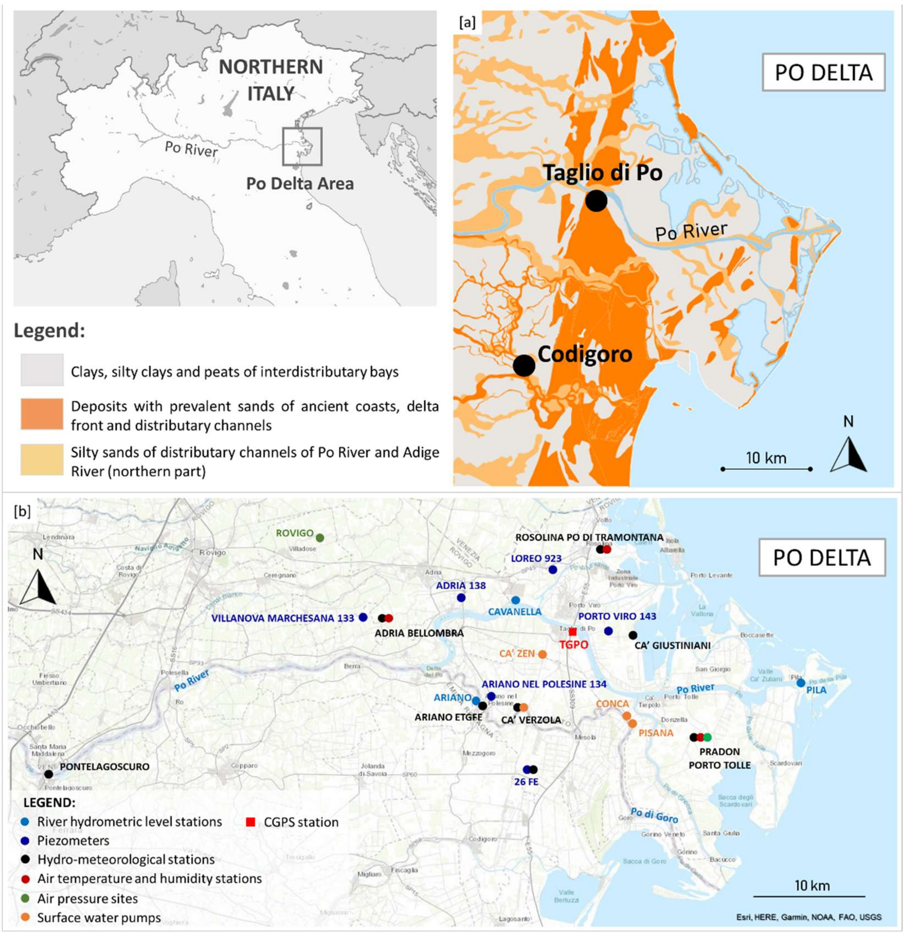
2. Po Delta Area (Northern Italy)

The Po Delta (Figure 1a) is one of the largest wetlands of Europe and belongs to the 701 most important Biosphere Reserves of the World [29]. The modern Po Delta results from the complex interplay between natural and anthropogenic processes [30] and owes its prominent shape to the artificial fluvial-mouth cut made at Taglio di Po (Figure 1a) in the early 17th century [31]. The Po Delta is a composite depositional system that comprises five main lobes built over an area of 380 km2 [32]. Sediments cropping out in the Delta (Figure 1a) are constituted by inter-distributary bay deposits of lower delta plain, marsh and lagoonal terrains, beach-ridge and aeolian dune sediments, which reveal present-day and ancient transitional environments [33]. The sediments that underlay the Po Delta exhibit a Late Holocene vertical succession characterized by transitions from prodelta muds to nearshore sands, and from delta front sands to lagoonal and swamps facies in the inner sectors of the Delta [34]. The shallower sedimentary sequence thus reflects the Delta progradation.
The Po Delta is fed by the Po River, the largest Italian river, which is characterized by a catchment area of 71,500 km2 extending over the Alps and the Northern Apennines [35]. The different climatic conditions that affect these chains influence the discharge regime of the tributaries and, as a consequence, the seasonal flow variability of the Po River main course. In particular, the Po River discharge measured at Pontelagoscuro hydro-turbiometric station (Figure 1b), which is located at 90 km upstream the river mouth, shows winter and summer depressions, and two peaks during late autumn and spring, due to intense rainfall and snow melt, respectively [36]. Furthermore, the Po River discharge annual means, recorded at Pontelagoscuro, and the rainfall annual means, collected into the Po River watershed, reveal a gradual decrease from 1975 to 2017 [37]. During the same period, the river discharge was characterized by drought episodes with river discharge lower than 500 m3/s, such as those which occurred in 2003, 2006, 2012, 2015 and 2017, and by numerous flood events with river discharge greater than 4000 m3/s. In addition, extreme flood events with river discharge greater than 6000 m3/s were observed in 1994, 2000, 2009, 2013, 2014 and 2016 [35,37].
Seasonal precipitation, distributed differently over the catchment, controls not only the river’s water regime, but also the sediment transport in the river. The terrestrial particles transported in the river water increase under cold and wet conditions and decrease during warm and dry conditions [38]. Correggiari et al. (2005) [33] indicate that during 1994 the sediment concentration of the river water passes from about 500 mg/L, during the wet periods, to 940 mg/L, during the flood events. Moreover, river regulations, dams and other anthropic actions affect both river water supply and sediment transport (e.g., [39,40].
With respect to the Earth’s surface deformations, the Po Delta is mainly affected by the land subsidence phenomenon [41]. Since the end of 20th century, measurements of ground level deformation started to be collected over the Po Delta area [42] and from 1950 repeated measures of spirit levelling were addressed to individuate the main subsidence causes [25,43,44,45]. Over the last decades, the introduction of high-precision levelling, differential InSAR, multi-temporal GPS surveys and their integration [27,28,46,47,48,49] favored a more complete and effective monitoring of the subsidence phenomenon over the entire Delta. The acquired datasets include the period of the intensive extraction of methane water from Quaternary deposits, which occurred from 1938 to 1961 causing significant land subsidence from the 1950s to the 1970s [41]. Afterwards, the ground lowering diminished still further and, at the present day, although reduced, it is still ongoing mainly due to natural processes [26,28,49,50]. Moreover, Fiaschi et al. (2018) [28] suggest that, over the Po Delta, the recently constructed buildings may cause the soil consolidation locally, thereby accelerating the natural subsidence.
The ground down-shift, due to the anthropogenic processes of the last century, reached, on average, 2 m of displacement and locally 3.5 m (e.g., [51,52]). Today, the Po Delta is largely located below sea level and is not exempt from flooding risk due to the sea, Po River and channels being used for reclamations. To protect the delta from this risk and to keep the water table at 0.5 m below ground level, a water management system is permanently used. It consists of 38 pumping stations and a drainage net 700 km long with a water extraction capability of 180 m3/s [30].

3. Data Presentation

The periodic component analysis of the VLM in the Po Delta is achieved by using the available geodetic, hydro-meteorological, hydrogeological and climate datasets (Figure 1b), and by applying a methodological approach recently proposed for evaluating subsidence in delta and coastal areas [24].

3.1. Geodetic Time Series

Site-positioning data used in this study are derived from a permanent station (TGPO) located in the Po Delta, 300 m away from the Po River, specifically at Taglio di Po village (Figure 1b). The station is composed of a Trimble GPS receiver that acquires data continuously with sampling rates of 1 second. It is located on a concrete block of a large building of the Po Delta Reclamation Consortium. The antenna is fixed to the structure, tightly connected to foundations located down to a depth of about 1.5 m below the ground level (b.g.l.), and measures displacements of the underlying soil, which consists of sands, silts and clays. North, East, and Up Continuous-GPS/GNSS (CGPS/CGNSS) components for the TGPO station were processed by two different organizations: Nevada Geodetic Laboratory (NGL) and Centro Interdipartimentale di Studi e Attività Spaziali, University of Padua, Italy (CISAS). Processed data were available from NGL GPS data system [53] and the Italian GNSS network. Since the horizontal components displayed negligible rates after removal of the Eurasia plate movement, only the vertical component of the ground deformation is analyzed herein.
The NGL data system is composed of about 17,000 GPS stations around the globe and is suitable for multiple purposes (e.g., tectonics and global sea level change). The data processing strategy is the precise point positioning, and the data products for each station (available online at http://geodesy.unr.edu/) are obtained using the GIPSY/OASIS-II software and are referred to the International Terrestrial Reference Frame 2014 [54]. The analyzed TGPO CGPS NGL (TCN) displacements run from 17 May 2007 to 10 June 2017. The obtained daily time series, appropriately cleaned from outliers, exhibit non-tidal loading effects (i.e., atmospheric pressure, ocean bottom pressure and hydrological loading) and show a site positioning uncertainty between 1.7 mm and 2.9 mm.
The Italian network is composed of about 700 stations distributed in Italy and in the surrounding European countries (about 30). Data processing uses standards recommended by the International GNSS Service and the EUREF GNSS European Permanent Network (EPN; [55]), and it is based on the double difference method. The stations’ coordinates are recalculated daily using the Bernese software [4]; the coordinates, updated in the reference system ETRS89 (European Terrestrial Reference System 89)/ETRF2000 (European Terrestrial Reference Frame 2000), are issued weekly by the CISAS from the adjustment of the 7 daily solutions with the use of precise orbits. At the TGPO station, the results are provided in terms of geographic and UTM (Universal Transverse Mercator, zone 33T) coordinates and ellipsoidal elevations. Thus, VLM of the TGPO station is obtained comparing the elevation in time. Elevation values are associated to the central day of each week and the analyzed TGPO CGNSS CISAS (TCC) data run from 17 April 2011 to 10 June 2017, derived from 1632 to 1952 GPS weeks. Data exhibit a site positioning uncertainty of 2–3 mm.

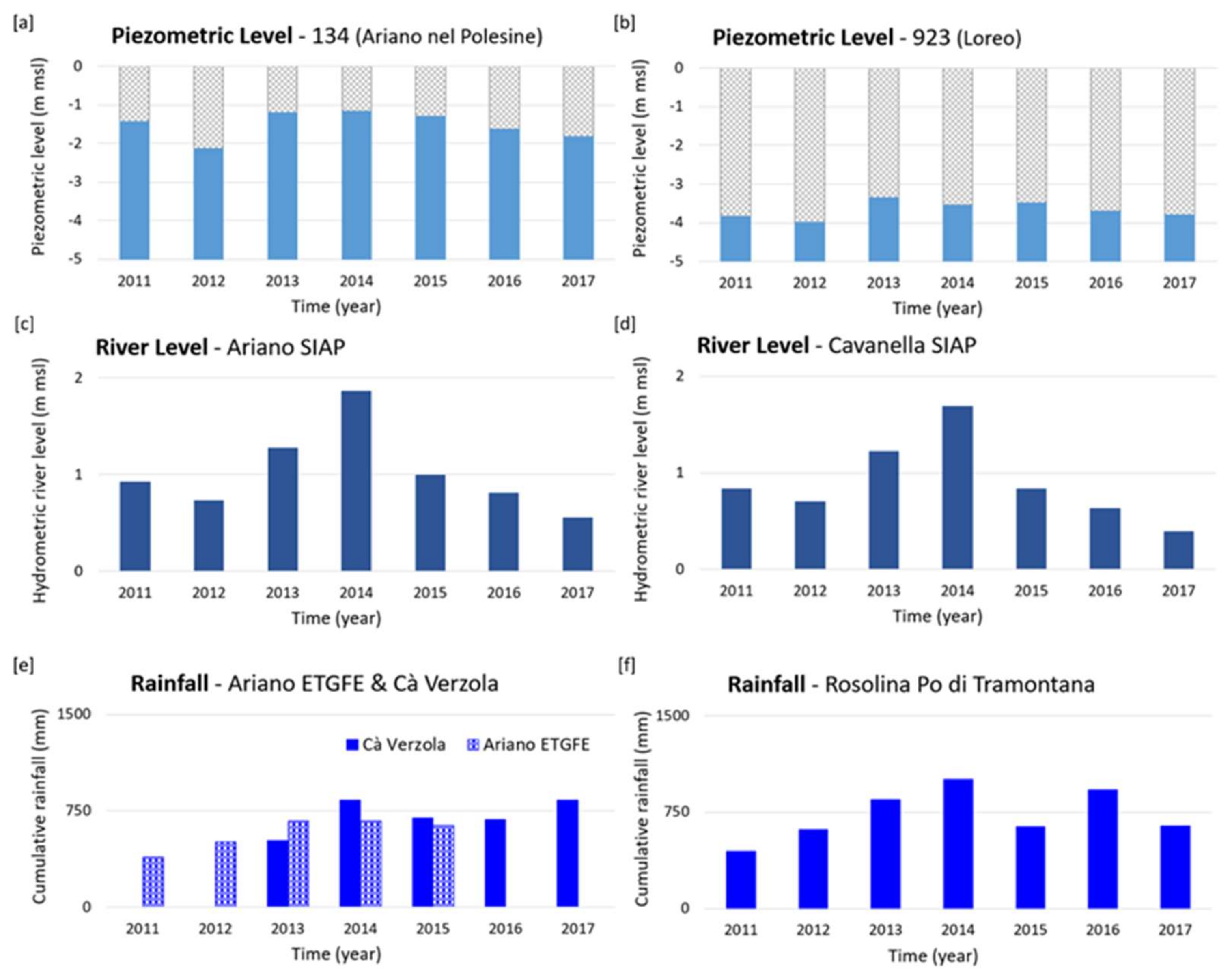
3.2. Hydro-Meteorological, Hydrogeological and Climate Datasets

The analyzed data, available on open-source websites or on request to the producing Institutions, refer to 7 different hydrological and climatic parameters collected from 19 stations located in the Po Delta area (Figure 1b). Table 1 summarizes studied parameters, provider websites, time intervals and analysis techniques of the datasets selected for each measurement station. Since time series coming from each station are inhomogeneous in terms of sampling rate and time span length, different analytical techniques are applied to recognize the main periodicities of the signals. It is worth noting that the higher the data frequency, the greater the advanced procedures, i.e., Wavelet Analysis (WA), Cross Wavelet Transform (XWT) and Wavelet Transform Coherence (WTC), were used instead of standard statistical techniques such as annual mean and Centered Moving Average (CMA) (see Section 4).

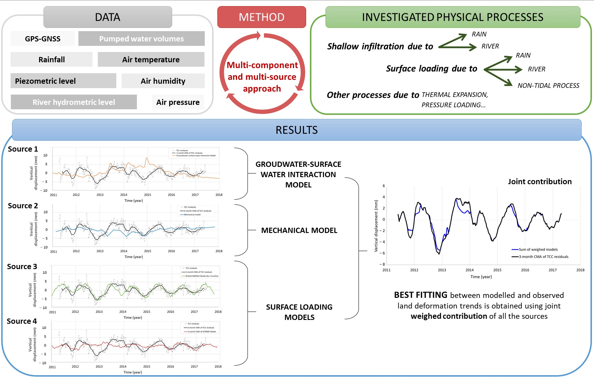
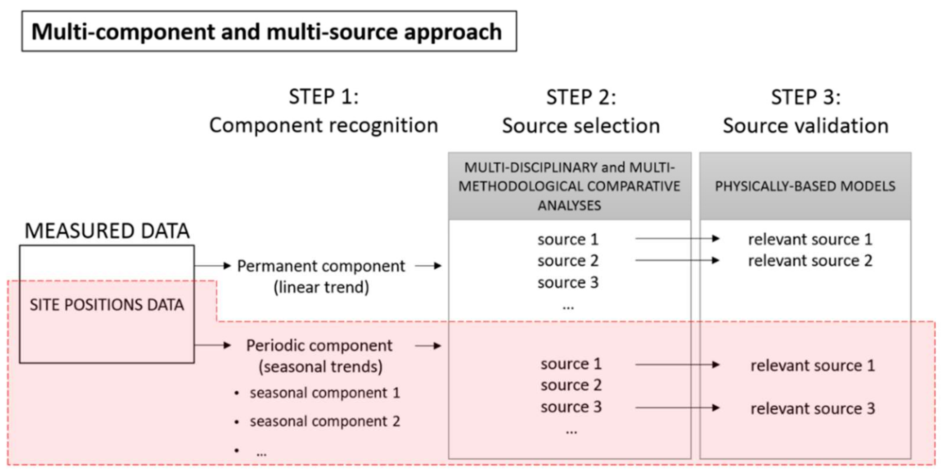
4. Application of the Multi-Component and Multi-Source Approach

The proposed methodology is essentially based on three main steps (Figure 2):
  • Step 1—once removed the permanent trend, moving average and wavelet analyses are applied to geodetic data for individuating the periodicity of the seasonal oscillations;
  • Step 2—comparative analyses, performed through statistic and wavelet techniques, are used to correlate the geodetic time series with datasets of different nature (e.g., hydro-meteorological and climate data). The purpose of this step is to find relations between land and hydrologic systems, and to infer the relevant sources among all those likely responsible for the observed land motion;
  • Step 3—the relevant processes are validated through physically based models.
It should be noted that the most suitable analytical technique to perform Steps 1 and 2 is chosen on the basis of the sampling rate of the analyzed time series, but also on the scale of the process to investigate. In particular, datasets with dense and constant sampling rates can be analyzed by wavelet techniques (WA, XWT, WTC), which simultaneously compare local amplitudes, frequencies, and phases of the signal patterns and provide multi-scale information [56]. In the presence of datasets characterized by inhomogeneous sampling rates, linear statistical techniques can be used (e.g., CMA [57]), which are often coupled with other functions, such as the natural smoothing spline, to extrapolate the obtained trends over the entire time length of the data. In the following Sections, the natural smoothing spline is also referred to as “smoothed CMA”.

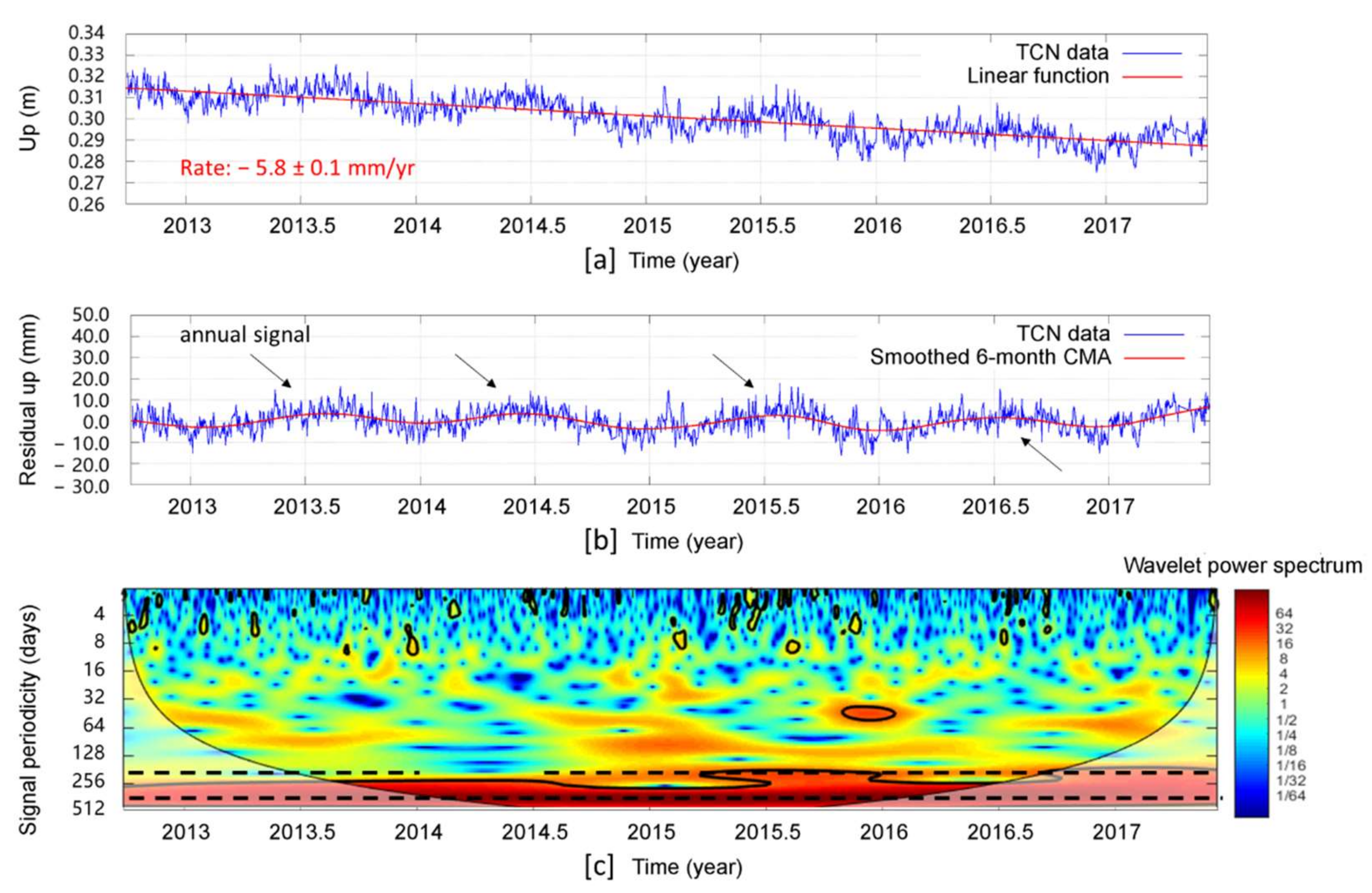
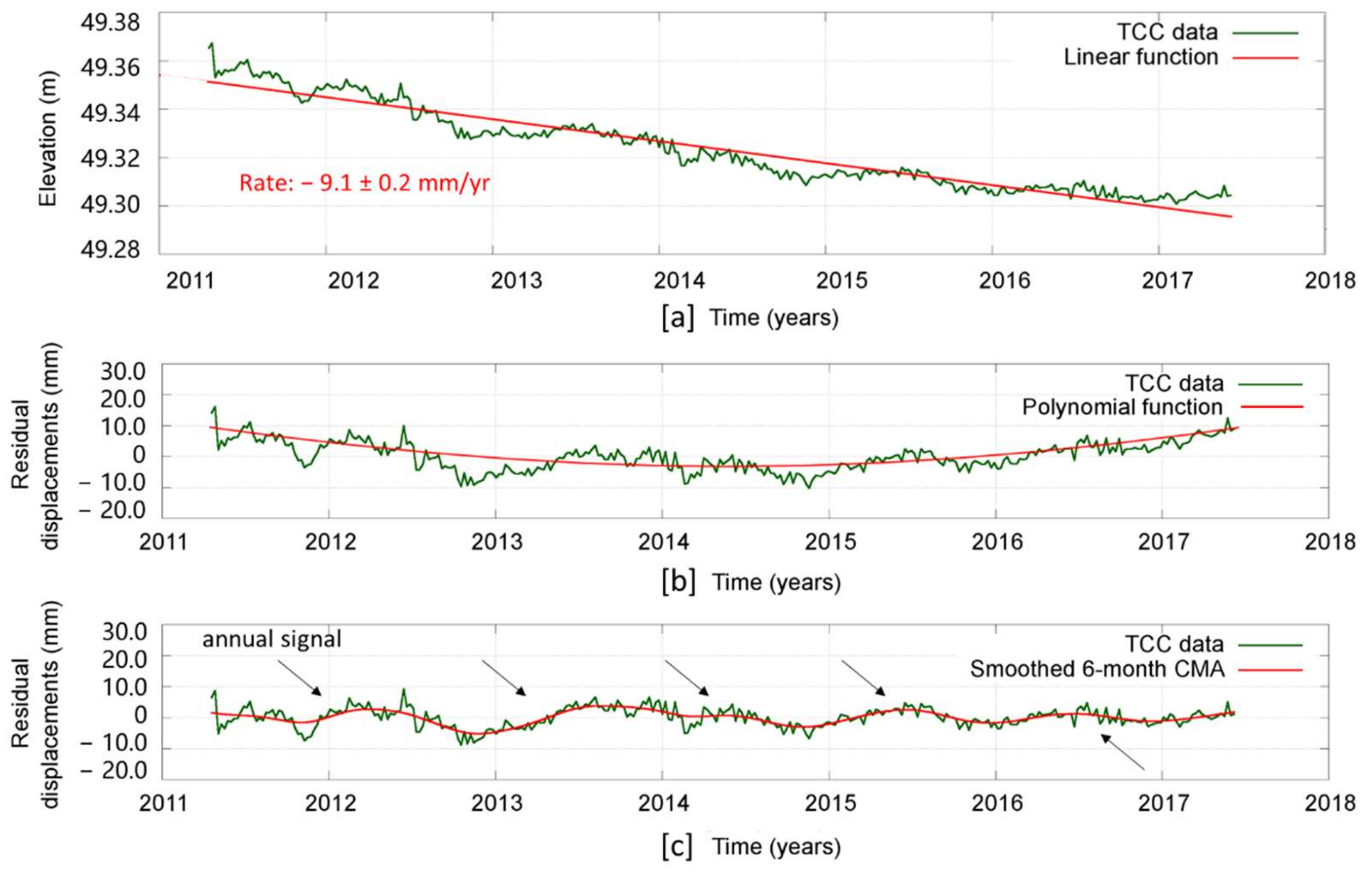
4.1. Step 1: Component Recognition of Geodetic Datasets

In order to individuate the main periodicities of the seasonal component, the two geodetic datasets are treated separately. Linear fit is performed first on the daily TCN data (TGPO CGPS NGL; see Section 3.1 for details) over a time period from September 2012 to June 2017 (Figure 3a). Then, it is applied to the weekly TCC data (TGPO CGNSS CISAS; see Section 3.1 for details) during a time interval ranging from April 2011 to June 2017 (Figure 4a). More details on the functions used for fitting data and the obtained parameters are given in Table 2. In particular, the preliminary geodetic velocity of −5.8 ± 0.1 mm/yr is computed for TCN time series within the analyzed time span (Figure 3a). Moreover, the natural smoothing spline, used for extending the CMA of a 6-month period over the analyzed data time span, points out the presence of a clear annual scale signal with maximum amplitude of 10 mm (Figure 3b). Wavelet analysis confirms the presence of a strong spectral power peak at 1 year (period = 365 days) and reveals also the occurrence of a weaker intra-annual oscillation at about a 6-month scale (period = 183 days; Figure 3c). Finally, weaker power picks at about 3-month (period = 96 days) and 2-month scales (period = 46 days) are also depicted within shorter data time spans, e.g., from 2014.5 to 2016.5 (Figure 3c).
The linear fit applied to the weekly TCC time series reveals a preliminary subsidence rate of about −9.1 ± 0.2 mm/yr within the time span April 2011–June 2017 (Figure 4a; see also Table 2 for details). Such a value is significantly higher than the velocity retrieved from the TCN dataset. The observed discrepancy can be due not only to the different analyzed time span (TCC dataset is longer than TCN one), but also to the different data processing strategies (precise point positioning method by NGL and the double difference method by CISAS) and to the use of different software (GIPSY/OASIS-II by NGL and Bernese by EPN) as argued by other authors (e.g., [58]). Further research could be implemented to better investigate these aspects and the incongruity on the permanent component of VLM in the Po Delta.
In the daily TCN time series the residuals of linear fit make the periodic patterns clearly visible, while in the linear post-fit residuals of the weekly TCC data a long-period signal still remains. Therefore, a polynomial fit of second order (quadratic equation) is applied on the weekly linear post-fit residuals (Figure 4b); the seasonal patterns can be clearly recognised removing the new fit from the residual series (Figure 4c; Table 2). The smoothed 6-month CMA applied on the quadratic post-fit residuals reveals the occurrence of a clear annual signal (Figure 4c) and confirms the periodicity already observed in the daily site-positioning time series of the TCN dataset (Figure 3b).

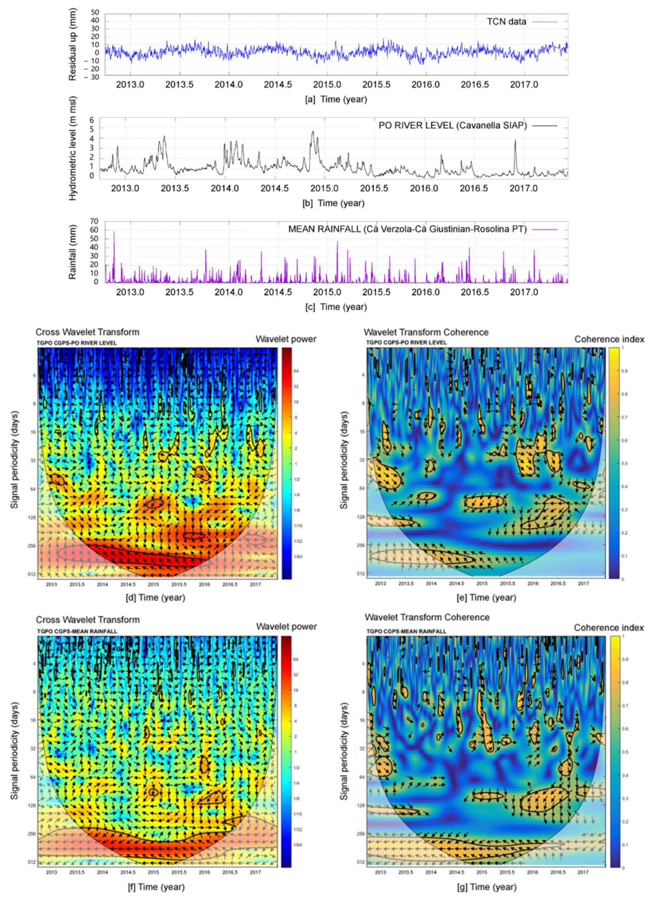
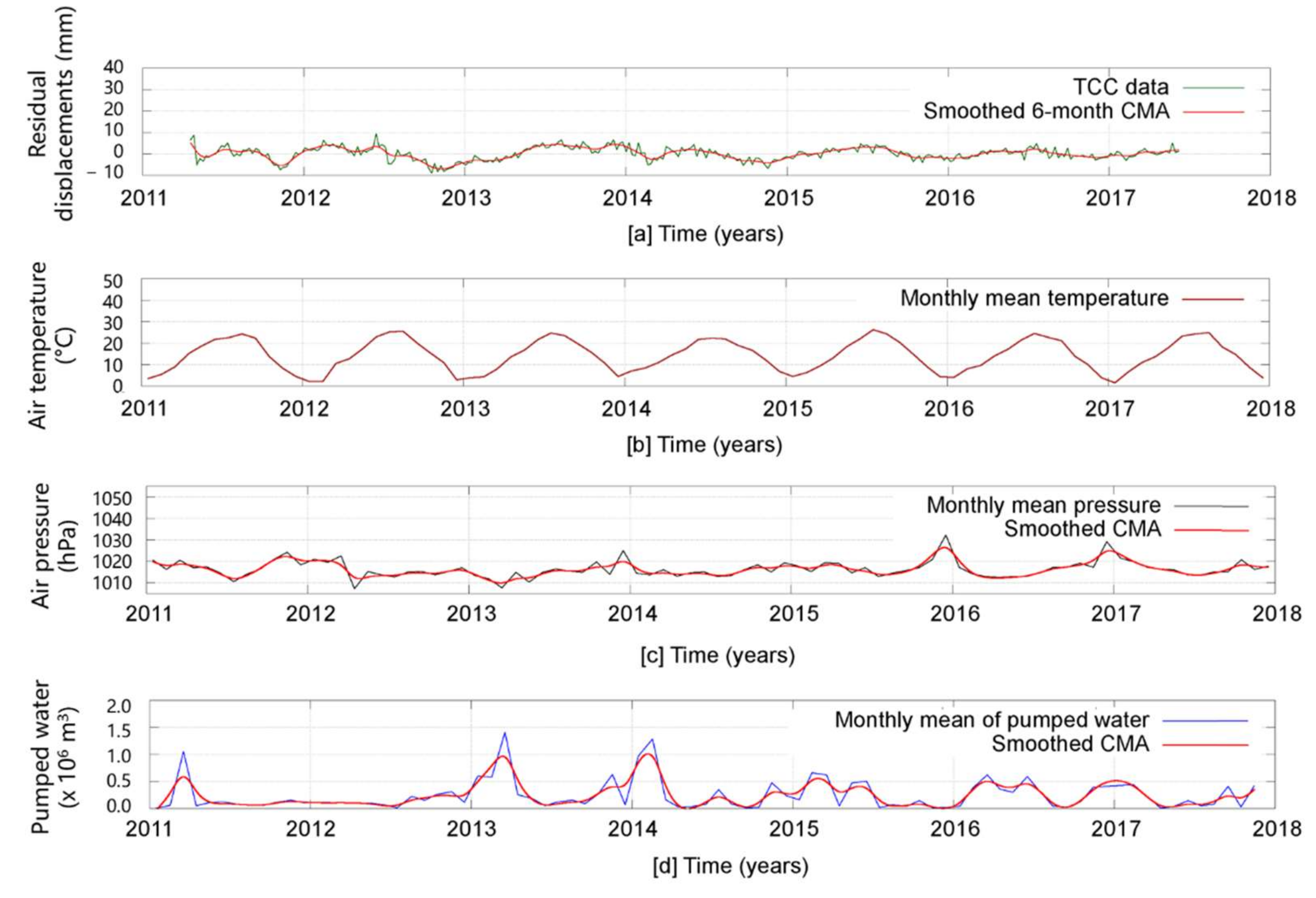
4.2. Step 2: Source Selection

Step 1 highlighted that the geodetic time series oscillations in the central part of the Po Delta are characterized by periodicities at annual (Figure 3b, Figure 4c) and intra-annual (6-month) scales (Figure 3c). Since these periodicities are typically found in the rainfall patterns [59], herein hydrogeological data (rainfall, hydrometric and piezometric levels) are analyzed to find correlations with geodetic data and for identifying possible physical processes (sources) that influence the land and surface/subsurface systems interplay. Moreover, in order not to exclude any mechanism responsible for the ground oscillations, other parameters (i.e., surface pumped water, air pressure and temperature) are also taken into account.
Before analyzing the daily datasets (geodetic data, river hydrometric stages, cumulative rainfall) through wavelet techniques, the available piezometric measures are compared with the hydro-meteorological time series using standard statistical methods. Due to the low sampling rate of the piezometric level (Table 1), these different datasets are compared by annual means. All the analyzed piezometers are installed in the shallow unconfined aquifer (aquifer A0, according to Emilia-Romagna Region classification). The oscillations of the water table and its capillary fringe might affect the GPS antenna, which is fixed to a shallow-founded building (<2 m b.g.l.). In particular, in the south west of the TGPO station (see also Figure 1b for location), the potentiometric level exhibited in the piezometer 134 (Ariano nel Polesine) reaches the minimum value in 2012, rising up to a maximum in 2014 and decreasing from 2015 to 2017 (Figure 5a).
The water table of the Po di Goro River measured at Ariano SIAP station (Figure 5c) rises from 2012 to 2014 and, in the same period, the rain amount of the Ariano ETGFE pluviometric station increases (Figure 5e). Despite showing similar behavior, the river hydrometric level trend better correlates with the piezometric level pattern during the period 2015–2017. Indeed, both these stations exhibit common decreasing trends. Moreover, in addition to the Ariano ETFGE rainfall station, which shows data up to 2015, the nearby Cà Verzola pluviometric station is also considered to observe the pluviometric trend from 2015 to 2017 (Figure 5e). This station shows that the annual mean of daily cumulative rainfall increases from 2016 to 2017. North of the TGPO station (see also Figure 1b for location), the piezometric level of the Loreo 923 site (Figure 5b) better correlates with the Po River level trend, measured at the Cavanella SIAP station (Figure 5d). Indeed, the rainfall quantity recorded at Rosolina Po di Tramontana pluviometric station increases until 2014, then drops off in 2015, reaching a new peak in 2016 and decreasing in 2017 again (Figure 5f). The Po River level recorded at Cavanella SIAP station displays a trough in 2012, reaching a peak in 2014 and then decreasing up to 2017 (Figure 5d). The river stage trend shows similarities with the piezometric level oscillation at the Loreo 923 site, since it exhibits a minimum value in 2012 and decreases from 2015 to 2017 (Figure 5b). The only difference is in the timing of the piezometric peak: it is reached in 2013 and not in 2014 (Figure 5b), as happens for the Po River trend (Figure 5d).
Figure 6 shows the results of a multidisciplinary comparative analysis performed through the Cross Wavelet Transform (XWT) and the Wavelet Transform Coherence (WTC) techniques on data spanning from September 2012 to June 2017. These techniques aim to find regions where the two considered simultaneous time series show high common power (XWT) and regions where the time-series covary but without having necessarily high power (WTC) [56]. In particular, the residuals of TCN time series (Figure 6a) are compared first with the daily Po River stage measured at the Cavanella SIAP hydrometric station (Figure 6b), and then with the daily mean of cumulative rainfall (Figure 6c). Precipitations are averaged over the available datasets of Cà Verzola, Cà Giustinian and Rosolina Po di Tramontana, which are the stations nearest to the GPS site (see Figure 1b for location). Figure 6d,e depict, respectively, the results of XWT and WTC between the geodetic time series and the river hydrometric level through time. The red areas within the cone of influence in Figure 6d reveal that, between 2014 and 2016, the geodetic trend and the hydrological pattern share a strong power peak at the annual scale (signal periodicity ~365 days). High wavelet power (red–orange-colored areas) is generally observed over the entire data time span (September 2012–June 2017) and associated to signal periodicities greater than 2 months (~64 days). In particular, high-power values are visible from 2015 in relation to signal periodicity at about a 6-month scale (~190 days). The annual signal depicts high wavelet coherence (green–orange- and yellow-colored areas) from 2012 to 2015, while the other signals, which are characterized by periods in between 3- and 6-month scales (between ~96 and ~190 days), show high coherence indexes referring to small and discontinuous analyzed time intervals (Figure 6e). In addition, at annual scale, where the wavelet power and the coherence indexes are more significant, the two records are close to the opposition of phase (by 180°), as revealed by the arrows directed to the left (by 135°). Such a result suggests a delay of one–two months between the two records. On the other hand, the signals are out of phase by 45°, 180°, 225°, 270° and 315° in period scales between 3- and 6-month. The scattered arrow directions for the intra-annual signals do not allow a clear interpretation of the relationships between the two records. Lastly, Figure 6f,g show, respectively, the results of XWT and WTC between the geodetic time series and the rainfall data through time. The strong wavelet power peak and the high coherence index found for the annual signal (periodicity ~365 days) indicate a clear 12-month correlation between the analyzed time series over the entire time span (September 2012–June 2017). The arrows pointing to the left (by 180°) reveal the opposition of phase between the two records. Moreover, the two signals are out of phase in the orange–yellow areas between 3- and 6-month scales of signal periodicity (between ~96 and ~190 days). In such regions, characterized by medium–high wavelet power and high coherence indexes, it is not easy to suggest relationships between the two analyzed signals, due to the scattered arrow directions.
Finally, Figure 7a–d show the comparison among the quadratic post-fit residuals of the TCC time series, the climatic data (air pressure and temperature) and the surface pumped water volumes, using smoothed CMA. All the analyzed climate and hydrological datasets are collected from available open-source websites; they are characterized by monthly sampling rates and are not uniformly distributed over the delta area (see also Table 1). In particular, the air temperature data shown in Figure 7b correspond to the mean of monthly cumulative temperatures collected from three stations widely distributed over the delta (Rosolina Po di Tramontana, Pradon Porto Tolle and Adria Bellombra stations; see Figure 1b for location). The air pressure data depicted in Figure 7c derive from the mean of monthly cumulative air pressures collected at two stations (Pradon Porto Tolle and Rovigo; see Figure 1b for location). Finally, the surface pumped water trend (Figure 7d) refers to the monthly volumes drained for managing the water surplus over the delta. The analyzed data were first collected from three sites located in between the Po and Po di Goro rivers (Cà Zen, Cà Verzola, Conca and Pisana sites; see Figure 1b for location) and then averaged to be representative of a wider delta portion. As can be seen in Figure 7, the thermal data show a clear annual oscillation that reaches maximum values during summer and minimum values during winter (Figure 7b). The pressure trend exhibits two evident peaks at the end of 2015 and 2016 (Figure 7c) and the pumped water trend is characterized by three peaks at the beginning of 2011, 2013 and 2014 (Figure 7d).
To quantify possible relationships among the analyzed signals, the linear correlation and cross-correlation functions implemented in Matlab (e.g., [60,61]) are applied on the monthly datasets (Table 3). The first technique provides the pairwise linear correlation coefficient (rho) and returns also the p-value, which tests the null hypothesis, that is no correlation exists between two considered signals. The higher (positive) the rho value, the more correlated the signals are. Moreover, a p-value less than the significance level of 0.05 rejects the null hypothesis. The second technique measures the correlation between two time series that are shifted of a lag. If the analyzed signals are normalized, the maximum correlation index is equal to one. The results of the correlation analysis shown in Table 3 clearly indicate that the ground level oscillation correlates only with the air temperature signal, even if the low values of the correlation parameters suggest a poor dependence between the two time series.

4.3. Step 3: Source Validation

Step 2 provided useful indications for selection of and modelling of the main physical mechanisms active over the central part of the Po Delta.
On one side, the comparative analysis based on standard statistical techniques (annual means) and applied to piezometric data collected near the main river courses revealed that the annual trend of the groundwater table better correlates with the river level variations (Figure 5). Since the GPS antenna is mounted on a building with foundations reaching the phreatic aquifer, the geodetic station might be affected by groundwater table oscillations. The proposed mechanism is successfully used to predict ground vertical deformation occurring in basins characterized by highly compressible deposits (e.g., [62]) or to match model results with observations acquired by satellite remote sensing techniques (e.g., [63]). To verify this hypothesis and to simulate the groundwater flow combined with the soil elastic strain, 3D modelling is performed. This process refers to groundwater–surface water interaction and mainly depends on water pressure. Modelling input and results are described in Section 4.3.1.
On the other side, the cross-wavelet analyses highlighted the occurrence of phase opposition between annual signals of the vertical land movement and hydro-meteorological data, suggesting the occurrence of loading processes. Ground level oscillation at TGPO station could be triggered by the elastic response induced by the changes of the Po River weight. To verify this second hypothesis and to simulate a mechanical process dependent on river water mass loading, 2D modelling is performed. Modelling input and main findings are presented in Section 4.3.2.
Moreover, the annual signals exhibited in geodetic and rainfall data were found in opposition to the phase (Figure 6f,g), thus suggesting, that when the rainfall amount is higher, the ground level is instantaneously lower and vice versa. Herein, the loading effect might depend on rainfall, soil moisture and canopy water changes, instead of surface water (including rivers) and groundwater processes. To verify this third hypothesis, three hydrological surface loading models were chosen and model findings are presented in Section 4.3.3.
Finally, since the quantitative comparative analysis based on correlation techniques did not reveal significant similarities between the TGPO geodetic trend and the other climate and hydrological data oscillations (Figure 7; Table 3), the occurrence of other sources, such as thermal expansion or atmospheric loading, have been excluded. This assumption is a pillar of the proposed approach (see Section 4), where the physically based modelling phase follows the analytical phase only if supported by the results of comparative analyses. It is important to note that the exclusion of other sources is also supported by further studies addressed to thermo-elastic expansion mechanisms and surface loading processes (e.g., [64]). On the other hand, the results of computational models provided by School and Observatory of Earth Sciences of the University of Strasbourg (http://loading.u-strasbg.fr/) confirm that at the TGPO station the atmospheric loading with the inverted-barometer ocean response (ATMIB model) and the ocean circulation effect (ECCO, ECCO2 models) are not dominant if compared with the hydrological contributions. Only the atmospheric loading, combined with the dynamic response of the ocean (ATMMO model), likely contributes to the Earth’s surface deformation and thus it is evaluated in addition to the continental hydrology load in the Section 4.3.3.

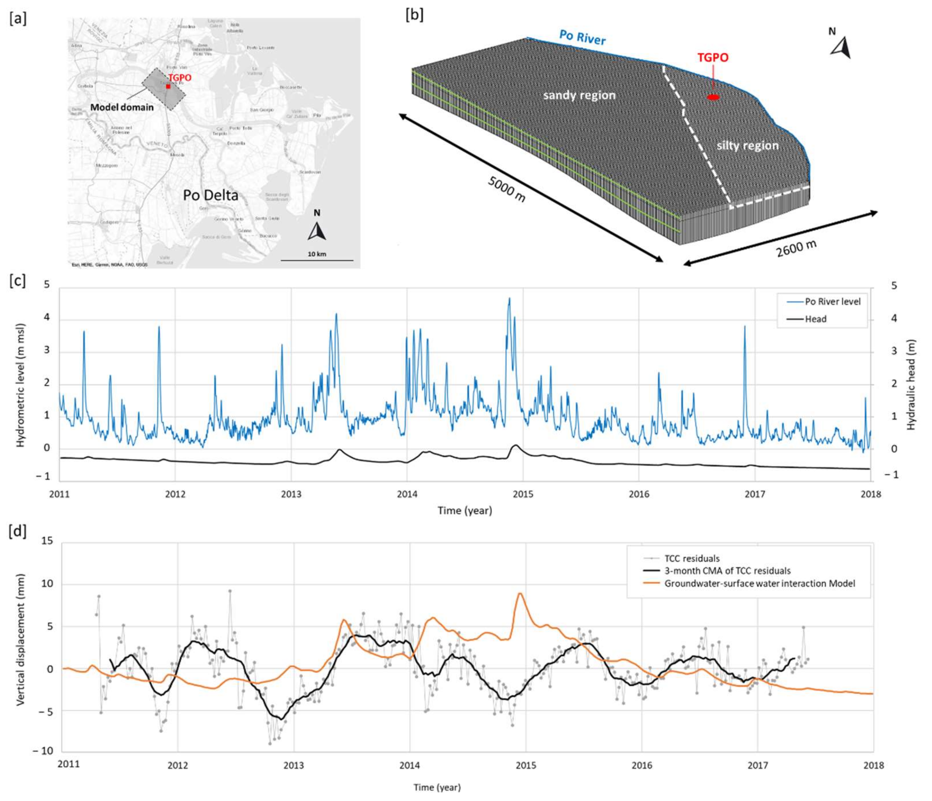
4.3.1. Groundwater–Surface Water Interaction

Groundwater–surface water interaction, and its potential effects in terms of VLM, was evaluated by a numerical approach using the Subsidence and Aquifer System Compaction Package (SUB) [65] associated with the modular three-dimensional finite-difference groundwater flow model (MODFLOW-2005) [66]. Starting from MODFLOW outputs, the SUB Package simulates recoverable (elastic) compaction or expansion, and permanent (inelastic) compaction of compressible fine-grained beds within an aquifer. Transient simulation was implemented to assess the relation between the oscillations exhibited in the TCC time series and the hydraulic head fluctuations induced in the phreatic aquifer by the discharge regime of the Po River, as suggested by the analytical results described in Step 2 (see Section 4.2). Since the current work is aimed at identifying the main sources responsible of the periodic signals of the surface land deformation, only the elastic component of VLM was considered in the numerical simulation. Future research will be addressed to investigate the physical processes controlling the permanent component of the geodetic signal.
The model domain sketches the main groundwater flow direction in the phreatic aquifer located south of the right Po riverbank (about north–south) (Figure 8a). The domain is a rectangle of 5000 m × 2600 m centered on the TGPO station and rotated 40° counter-clockwise from the north direction. A uniform spatial grid is designed using a horizontal cell size of 20 m × 20 m, from which derive 230 columns (X-dimension) and 130 rows (Y-dimension). The vertical discretization is composed by two horizontal layers: the upper one of constant thickness (layer 1), equal to 5 m, and the lower one of variable thickness (layer 2). These layers are included between the ground surface, which is approximately at 0 m above mean sea level (a.m.s.l.), and the base of the Holocene prograding deposits (i.e., the sandy aquifer A0, see Section 2), which ranges from −8 m to −25 m a.m.s.l. Layer geometries were derived from geological information, available on the surface Geological Map Sheet 187 [67], and from litho-mechanical data referred to 17 boreholes or piezocone tests within the Taglio di Po area, available on the Emilia-Romagna Region website (http://ambiente.regione.emilia-romagna.it/geologia/cartografia). Moreover, according to the outcropping lithologies, the upper layer is divided in two litho-type zones, described below through specific petro-physical, mechanical and hydraulic properties. After the deactivation of the portion of grids located north to the Po River, the model domain is composed of 54,306 active cells.
The total simulation time length is 2552 days, from 1 January 2011 to 31 December 2017. This time is divided into 366 stress periods of variable amplitude, from 1 to 7 days, and the 1st stress period (1-day length) runs in steady-state to adapt the initial head distribution to the transient boundary conditions.
To simulate the elastic VLM in transient regime, specific model parameters are defined: (i) hydraulic conductivity (K) along the three axis of discretization (Kx, Ky, Kz); (ii) specific yield (Sy) for partially saturated cells; (iii) specific storage (Ss) for saturated cells; (iv) elastic skeletal storage coefficient (Sfe) derived from compressibility (α) and thickness of the medium. In the entire model domain, K, is considered as an isotropic property both in the horizontal plane (Kx/Ky = 1) and in the vertical direction (Kx/Kz = 1). In layer 1, two different zones are defined (Figure 8b): the region with silty-rich deposits (silty aquitard), which identifies the south-eastern part of the model domain, and the region with sandy deposits (sandy aquifer), which characterizes the remainder of the grid. Layer 2 is defined only by the sandy aquifer. Table 4 summarizes the main model parameters assumed for the two layers in accordance with the mechanical parameters used in the river water mass loading simulation. In particular, Ss is derived from the compressibility α, which is the inverse of the Young’s modulus, by the equation:
S s = ρ g α + n β
where n is the porosity of the medium, g is the acceleration of gravity, ρ and β are the density and compressibility of the water, respectively.
With respect to the boundary conditions (BCs), groundwater–surface water interaction is reproduced using the RIVER Package of MODFLOW (Cauchy BC or 3rd type BC) applied to the cells placed along the north-eastern border of the grid (Figure 8b). The river stage associated with this BC decreases progressively from north-west to south-east and is derived from the hydrometric level recorded at the Cavanella SIAP and Pila SIAP stations for the simulation period (see also Figure 1b for location). The riverbed conductance is computed starting from a specific value of 0.1 m/s to favour an adequate interaction between the river and aquifer. A realistic hydraulic gradient is guaranteed applying the DRAIN Package of MODFLOW (Cauchy BC or 3rd type BC) to the south-western border of the model domain (Figure 8b). The drain elevation associated with this BC is equal to −4.5 m a.m.s.l., while the drain conductance is computed starting from a specific value of 10 m/s. Finally, three No-Flow BC (Neumann BC or 2nd type BC) are applied at the north-western and south-eastern borders and at the bottom of the model domain, respectively (Figure 8b). The infiltration due to rainwater is considered negligible compared to the river–aquifer exchange flux, and for this reason no BCs are used on the top of the model domain to simulate the recharge due to infiltration processes.
With respect to the hydraulic head computed in correspondence of the TGPO site, it is clearly related to the Po River hydrometric level at Cavanella SIAP station (Figure 8c), as well as being comparable in terms of magnitude and trend with the values of hydraulic head recorded in the piezometers 923 and 134 (see also Section 3.2 and Figure 1b for location), situated outside the model domain in quite similar hydrogeological conditions.
Figure 8d shows the model results compared with the geodetic observations at the TGPO site. Although the computed elastic VLM is comparable in terms of the oscillation amplitude to that exhibited in the residuals (original weekly site-positioning data detrended by linear and quadratic fits; see also Section 4.1 for details), it mismatches the observations since it appears in opposition of the phase when compared with the measured ground level. An exception to this behaviour is observed during April–May 2013 and July–August 2015, where the geodetic signal seems to be consistent with the calculated displacement, as well as in 2016, where the computed trend matches the signal phase and smooths the amplitude of the geodetic observation.
In order to evaluate the model accuracy, a quantitative approach was used by considering some statistical parameters calculated on the residuals between the observed and simulated displacement. The observed displacement corresponds to the 3-month CMA fit obtained from the quadratic post-fit residuals of TCC data (see also Section 4.1 for details). The chosen statistical parameters are the Root Mean Square Error (RMSE) [68], the Normalized Root Mean Square Error (NRMSE) and the Nash–Sutcliffe efficiency (NSE) [69]. As is well known, the RMSE is one of the most used statistical error indexes and it is commonly accepted that the lower the RMSE, the better the model performance. NRMSE is calculated by normalizing the RMSE based on the range of the observed data. NRMSE is often expressed in a percentage, and 10% is the calibration criterion frequently used in hydrogeology [70]. NSE ranges between −∞ and 1.0, with NSE equal to 1 being the optimal value. Values between 0.0 and 1.0 are generally considered as acceptable levels of performance, whereas values <0.0 indicate unacceptable results [68]. In the groundwater–surface water interaction case, the values of 3.48 mm, 34.60% and −1.34 for RMSE, NRMSE and NSE, respectively, highlight a poor performance of the model.

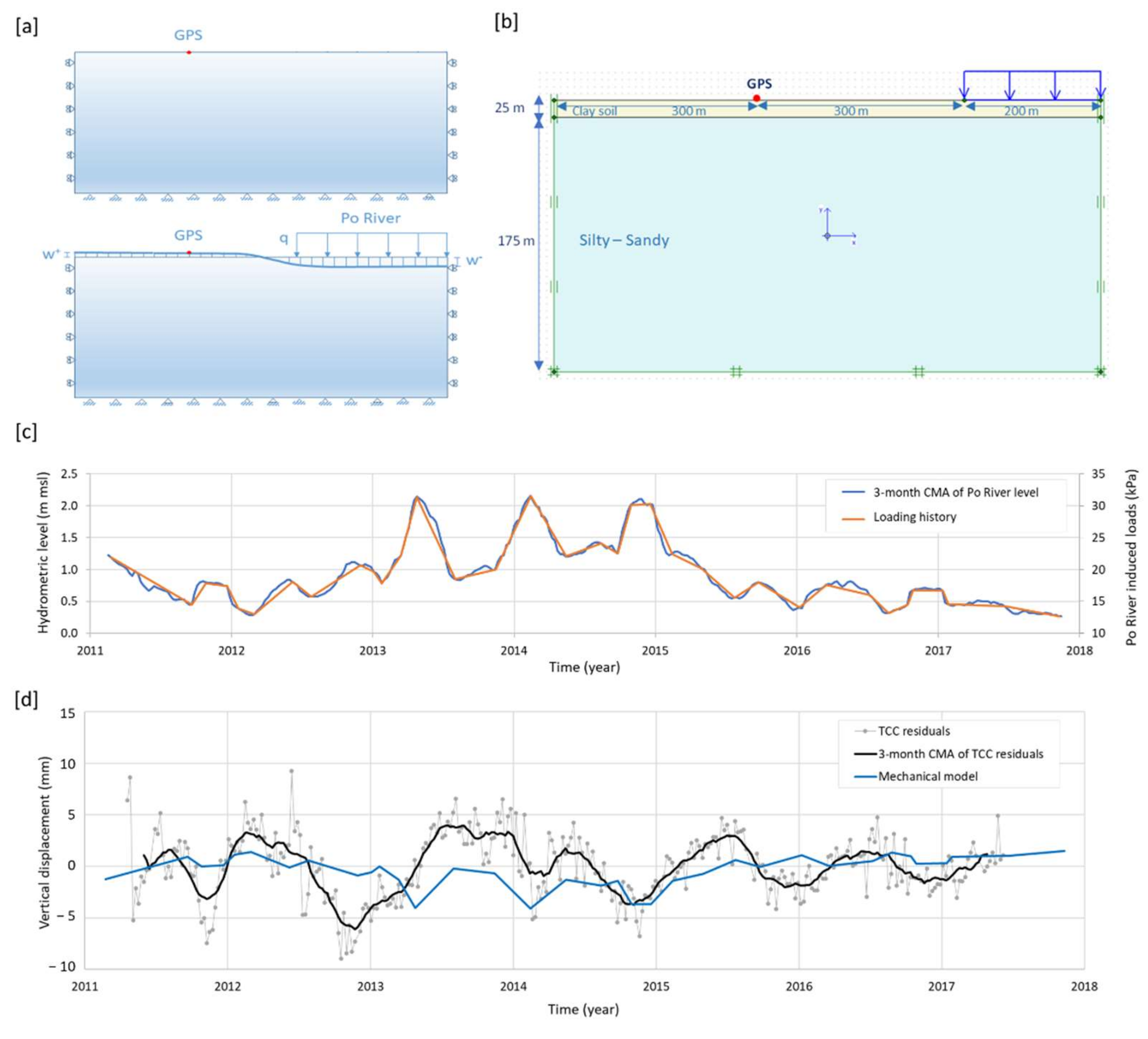
4.3.2. Mechanical Modelling via FEM

The effects induced by the Po River loading variations on the ground surface at TGPO site were evaluated through a mechanical modelling based on the finite elements method (FEM). Specifically, the PLAXIS 2D software (Bentley Systems, Inc., Exton, PA, USA) is used, which is commonly employed in geotechnical engineering for the analysis of soil deformation coupled with groundwater flow.
The main input of the simulated process is the river level fluctuation: over time, the river height oscillation induces the variation of the hydrostatic water pressure acting on the riverbed, which in turn induces deformations into the shallow sedimentary layers. The proposed model is an elastic continuum medium that, under load variations due to river height fluctuations, causes ground surface movements. Due to the relative rapidity of the river fluctuations compared to the hydraulic conductivity of the shallow layers, undrained conditions of the subsoil are assumed. Therefore, no flow is simulated in the model layers, and the strains, whose magnitude depends on layer stiffness, are considered as purely distortional. As schematically shown in Figure 9a, with respect to the initial condition without loading on the model surface (upper sketch), the increase in the river water loading on the riverbed due to the hydrometric level rise (lower sketch) increases the downward vertical land movement (subsidence due to settlements) below and close to the overloaded riverbed, and uplifts ground level far from the loading area.
This distortional effect is simulated by a 2D subsurface model consisting of a cross section along the Po River near to Taglio di Po village, which includes the TGPO GPS antenna. The model is 800 m wide and 200 m deep and is characterized by two layers (Figure 9b): the upper one has a constant thickness of 25 m and is constituted by silty sand deposits (layer 1) and the lower one has a constant thickness of 175 m and is made by sandy deposits (layer 2). The mechanical parameters of the layers were calibrated to reproduce the magnitude of the measured settlements at the ground level. In accordance with the calibration procedure, the final physical and mechanical properties of the two layers are shown in Table 5.
The loading history, which represents one of the main model inputs, is derived from the Po River hydrometric level measured at Cavanella SIAP station (see Figure 1b for location) from 1 January 2011 to 31 December 2017 (Figure 9c). In particular, to simulate the long-term loading trend, the 3 months CMA fit applied on the river level data is used.
The computed vertical displacements of the ground level at the GPS antenna site compared to the measured TGPO displacements (Figure 9d) show that the latter are consistent with the undrained distortions of the ground surface induced by the river loads. In the period March 2013–September 2017, the model findings reproduce well the observations, indeed the oscillation phases are matched, and the simulated amplitudes are comparable in terms of magnitude. For the periods June 2012–March 2013 and September 2015–February 2016, the computed settlements show opposite phases with respect to the measured ground level displacements.
Finally, the accuracy of the mechanical model is evaluated as in the previous section by the statistical parameters. Indeed, values of 2.49 mm, 24.74% and −0.20 were found for RMSE, NRMSE and NSE, respectively; they indicate an improvement of the match between model and observation with respect to the groundwater–surface water interaction simulation.

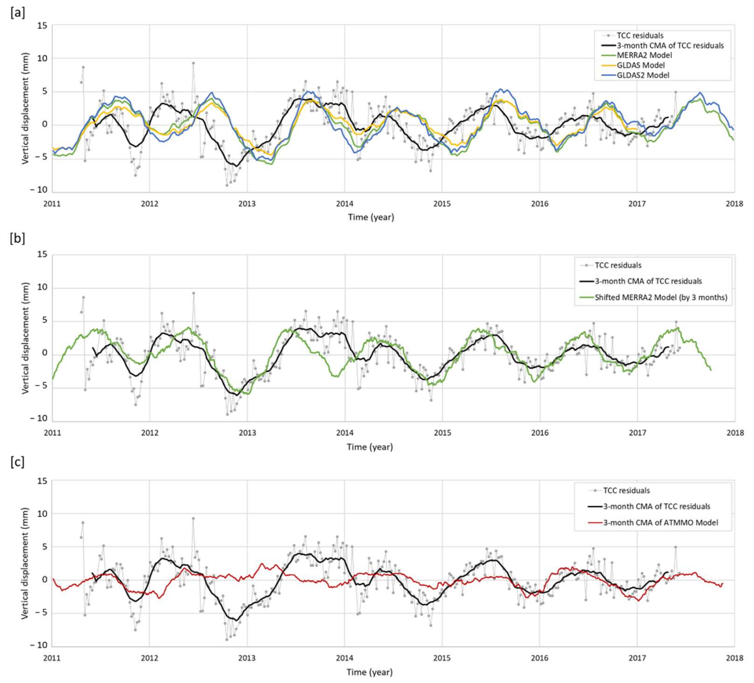
4.3.3. Models of Global Mass Variability in Atmosphere, Ocean and Continental Hydrology

The displacements computed at the TGPO site on the basis of the global mass variability in atmosphere, ocean and continental hydrology were provided by the loading service of the School and Observatory of Earth Sciences of Strasbourg (http://loading.u-strasbg.fr/). The service center delivers 3-D (North, East, Up) surface displacements computed by using global atmospheric, oceanic and hydrological circulation models (e.g., [71]).
In particular, the hydrology loading chosen for this study was estimated from GLDAS/Noah (version 1 and 2.1) [72] and from MERRA 2 models [73], whose surface displacement time series have been available since 2000. GLDAS/Noah models allow for soil moisture, snow and canopy water, and are characterized by spatial and temporal resolutions of 0.25° × 0.25° and 3 hours, respectively. MERRA2 model accounts for soil moisture and snow, and the spatial and temporal resolutions are 0.50° × 0.63° and 1 hour, respectively. Details on the main model input parameters (e.g., soil properties, soil moisture, layer thicknesses) can be found in Reichle et al. (2017) [74]. The deformation mechanism does not account for groundwater processes and surface water, including rivers. For our purposes, only the vertical component (Up) at the TGPO site was selected within the time interval comparable with the period of geodetic data analysis (January 2011–December 2017). The displacement time series (MERRA2, GLDAS and GLDAS2) at the TGPO site, picked up from the global database, were resampled at a weekly rate applying the decimate function, an operator of signal processing implemented in the Matlab package software, which modifies the sampling rate by the integer factor using a Chebyshev filter. Comparison between model findings at the TGPO site and TCC data are shown in Figure 10a. It is worth noting that GLDAS results are available up to December 2016 and, thus, do not entirely cover the studied period.
Although the three modelling results slightly differ due to model input (e.g., layer geometry or land surface model), all the model findings fit the residual data well in terms of signal frequency and amplitude (Figure 10a). In fact, all the models clearly simulate oscillations of annual period and exhibit amplitudes ranging from 6 mm to 10 mm, plus other weaker fluctuations at intra-annual scales. Conversely, the computed trends reveal an evident signal phase lag of about three months, likely due to the local conditions. In fact, specific lithological or petro–physical characterizations at the TGPO site are not considered in the model since the model mesh covers the entire Po Delta. This aspect will be also tackled in Section 6.
Moreover, the selected hydrological models (MERRA2 and GLDAS2) show poor correlation with the geodetic signal mainly due to the phase lag, as is highlighted by the high values of RMSE and NRMSE correlation coefficients and by the negative NSE values (Table 6). To better correlate model results and geodetic data and to find the time intervals where the simulated trends overestimate or underestimate the geodetic signal, the computed displacements are corrected reducing the phase lag to zero. Afterwards, phase-shifted MERRA2 and GLDAS2 models, which cover the entire analyzed period (January 2011–December 2017), underwent the residual analysis between computed and observed displacements by using again statistical indicators (Table 6). This last analytical phase pointed out that MERRA2 provides better agreement with the observations than GLDAS2. However, although MERRA2 presents the lowest RMSE value and a NSE within the acceptability range, NMRSE still remains above the calibration threshold (Table 6).
Figure 10b depicts the good match between the phase-shifted MERRA2 model and the geodetic trend, but also highlights the occurrence of a clear discrepancy at the end of 2013, and other short gaps during the analyzed time interval.
With respect to the non-tidal atmosphere and ocean contributions, the ground displacements at TGPO site were estimated from the ATMMO model, which considers European Center for Medium-Range Weather Forecasts (ECMWF) and assumes a barotropic oceanic response to pressure and winds, using the TUGO-m model [75]. The ATMMO model provides 3-D displacement maps on 3-hourly and 0.25-degree grids [71], plus time series since 2002. Herein the displacements through time are presented from January 2011 to November 2017 (Figure 10c). As is shown in Figure 10c, the non-tidal loading effects are not relevant at the TGPO site, since the mean signal amplitude of the ATMMO model corresponds to 1 mm and is much lower than those exhibited by the geodetic time series (5–6 mm). Moreover, the ATMMO model phase is not in line with the geodetic signal during the 2012–2015 period. Finally, the poor correlation between the modelled signal and observations is also confirmed by the high RMSE and NRMSE values, and by the negative NSE values shown in Table 6.

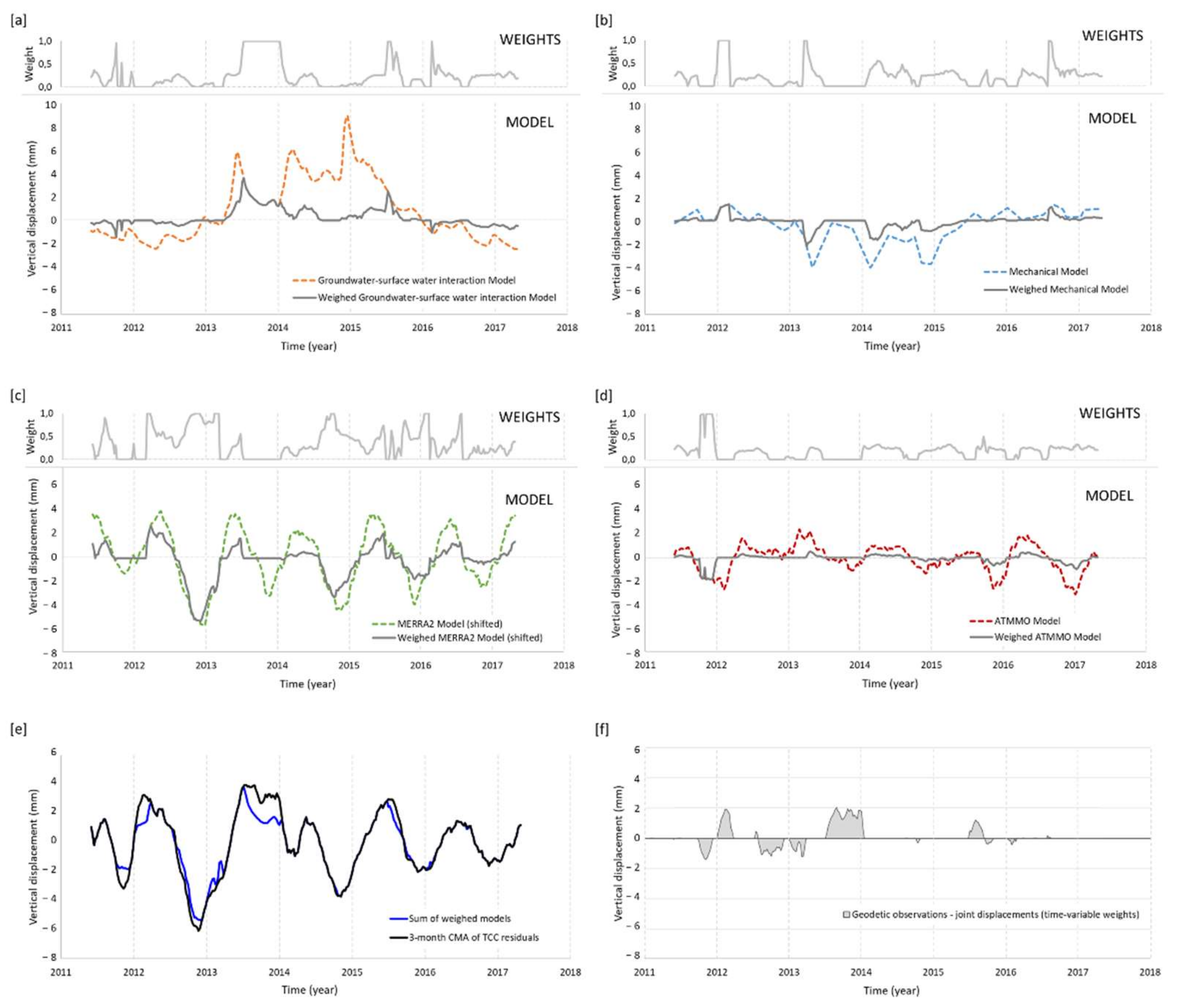
5. Joint Contribution of the Proposed Sources

To evaluate the joint effects of the modelled sources, the sum of displacements com-puted by each individual source (joint displacements) are compared with the observed geodetic displacements by using statistical parameters. The quantitative evaluation was conducted according to three different scenarios. In the first case, the superposition principle is applied to calculate the total displacement as the sum of the single simulated components. In fact, several examples available in the literature point out the role of this principle for the estimation of land subsidence [76,77,78,79]. In the second and third cases, the sum of the displacements due to each source is weighed by using constant and time-varying weights, respectively. In these two scenarios, the weights, not defined a priori, are estimated by the Generalized Reduced Gradient (GRG) method [80]. Such a technique is based on an optimization algorithm commonly used for solving nonlinear problems and recently applied in hydrology (e.g., [81]) and hydrogeology (e.g., [82]). The optimization procedure was conducted by minimizing the sum of squared residuals between observed and calculated displacements, and a sum of weights equal to one was used as constraint during the optimization process. Specifically, the computed time-constant weights for the second scenario are: 0.59 for the hydrological loading source, the 0.27 for river-water mass loading source and 0.14 for the groundwater–surface water interaction source, while no contribution is attributed to the non-tidal loading source (null weight). The computed time-variable weights related to the third scenario are shown in Figure 11a–d. Their mean values correspond to 0.36 for the hydrological loading source, 0.21 for river-water mass loading source, 0.25 for groundwater–surface water interaction source and 0.18 for non-tidal loading sources. Comparing the second and third scenarios, it should be noted that the use of time-variable weights diminishes the role of the river-water mass loading process and increases that of the groundwater–surface water interaction. This observation is also confirmed by the residual displacements shown in Figure 11e,f, which are obtained removing the joint displacements, calculated according to GRG method and time-variable weights, from geodetic observations. Although the joint contributions of the four models generally match with the observations, four clear exceptions can be identified in late 2011–early 2012, late 2012–early 2013, the second half of 2013 and mid-2015 (Figure 11f). In particular, the discrepancies revealed in late 2011 are reducible by varying the weights of the river water mass loading and groundwater–surface water interaction contributions, whilst those observed in mid–2015 are reducible by varying the weights of all the contributions. In contrast, the remaining discrepancies, and especially those that occurred in the second half of 2013, are irreducible, suggesting the presence of additional non-dominant processes that have not yet been recognized.
Finally, regarding the accuracy of the model–observation match, the statistical parameters RMS, NRMS and NSE retrieved for each scenario (Table 7) indicate that the observed displacement is better described by a time-varying combination of the four phenomena (third scenario).
In addition, the Person’s correlation coefficient (R) (e.g., [83]) in Table 7, which characterizes the linear relationship between computed and observed displacements, increases from the first to the third scenario and confirms the better result achieved under the third hypothesis of time-variable weights.

6. Discussion

Surface displacements provided by the first simulation (Section 4.3.1) were due to the groundwater level fluctuations induced in the phreatic aquifer by the changing of the Po River hydrologic regime. Generally, modelling results are not in line with the ground level variations measured during April 2011–June 2017 period. The only exception is in 2016, where the computed trend matches the signal phase and partly reproduces the amplitude of the geodetic observation (Figure 8d). Model findings seem to be also consistent with the rise and fall of the geodetic signal which occurred in April–May 2013 and July–August 2015, respectively. Moreover, although the comparative analysis based on annual means suggested a river–aquifer exchange process driven by river water fluctuations and active at the annual period scale (Figure 5), model findings do not support this hypothesis, while suggesting the occurrence of fluxes exchange during short periods or at intra-annual scale.
Surface distortional deformations computed in the second numerical model (Section 4.3.2), which considers the loading history induced by the river water mass change during the analyzed time interval, simulate well the sequence of peaks and troughs at inter- and intra-annual scales exhibited by the geodetic signal. Conversely, such deformations do not match with the ground level depression visible at the end of 2012, and with the intra-annual oscillation (6-month period scale) localized from October 2015 to October 2016 (Figure 9d). The computed amplitudes range from 1 mm to 5 mm of height, while the observations vary from 2 mm to 10 mm (Figure 9d). This discrepancy might be due to the preliminary water density used as model input, which does not consider suspended matter in the river water. Indeed, as mentioned in Section 2, several authors suggest that in the Po River prodelta such materials vary significantly in space and time, according to hydrological and meteorological events (e.g., [35]). During dry periods, water turbidity can reach values lower by an order of magnitude than those observed in flood conditions. As consequence, the change of the river water weight due to seasonal variations of suspended matters is particularly evident when the transition from dry periods to flood events occurs, and it might amplify the strain due to the river water loading on the ground level. With respect to the results of the comparative analysis based on the wavelet techniques (Figure 6d,e), model results do not support completely the loading hypothesis suggested by the analytical correlation results. Indeed, the phase opposition found between the TCN data and Po River hydrometric level measured at the Cavanella SIAP station indicates that, when the Po River is higher, the ground level is lower (with a delay of one-two months). Conversely, due to the strain field generated by the river loading and to the distance of the GPS site with respect to the river axis, modelling results indicate that, when the Po River is higher, the ground level in correspondence of the GPS antenna location is also higher. Signals in phase opposition (i.e., high river level correlated with simultaneous low ground level) can be found only in the model cells located close to the river boundary.
The displacement pattern obtained by the third modelling and, in particular, by MERRA2 (Section 4.3.3), is not in agreement with the TCC residual time series, mainly due to a time-lag of three months (Figure 10b). Although the origin of the constant phase discrepancy between computed and observed signals is not clear, it can be likely attributed to the mesh size and properties of the model. Indeed, due to model resolution, the entire delta corresponds to one grid mesh and, therefore, key properties affecting the infiltration process in the canopy and shallow layers, as well as the soil texture or the rainfall amounts, are considered homogenous over the entire delta, while they are significantly different at the local spatial scale. As observed in the southern part of the Po Delta [24], where a similar phase-lag was found in 2014 by comparing a TCN time series with the results of hydrological models, the rainfall amounts in the north-western part of the Delta differed substantially from those in the eastern and southern parts. The timing of local precipitation could justify short periods of delay in water infiltration. However, considering the phase-shifted MERRA2 hydrological model, the results match with the geodetic trend, except for the July–December 2014 period, and slightly overestimate the signal amplitude during April–May 2011, 2016 and 2017. All these periods could be related to seasonal fluctuations of the Po River: during 2014, the Po River experienced flood and extreme flood events, while dry periods occurred in early 2011 or mid-2016 and 2017 (Figure 6b). In addition, the original TCC time series shows gaps and outliers at the beginning of 2011 and thus the CMA computed on the TCC data can be fictitious during that time interval. Concerning the wavelet analysis results shown in Figure 6f,g, the phase opposition found at annual scale between geodetic signal and rainfall data indicates that the higher the rainfall is, the lower the land surface is and vice versa. This result is in accordance with the simulated hydrological loading mechanism.
The latest simulation, which is based on the atmospheric loading combined with the dynamic response of the ocean (Section 4.3.3), predicts mean surface displacements that are 1/3 smaller than those calculated from the hydrological loading (Figure 10b,c). As already suggested by other authors (e.g., [84]), this outcome is expected when the computational periods are particularly long. Indeed, computed surface displacements of hydrological and non-tidal loading models are available from 2000 and 2002, respectively. However, despite the small contribution given from this model to the geodetic signal, the proposed mechanism was treated as a joint contribution to the other processes.
With respect to the joint contribution of the proposed sources (Section 5), the obtained results show that the observed displacement is better described by a time-varying combination of the four phenomena (third scenario in Table 7, and Figure 11e,f). Moreover, although the hydrological surface loading seems to be the main source of the vertical land displacement, the role of the river-mass loading process and the groundwater–surface interaction increase during specific periods, such as the Po River wet phase that occurred in 2013–2014 (Figure 11a–d).
Finally, in the light of these latest findings as well, it appears that, where the hydrological loading model fails, the other proposed models give relevant contributions. Specifically, during the wet period of the Po River (2013–2014), the mechanical model based on the river loading simulates quite well the peaks exhibited in the geodetic trend, while in the dry periods (2011–2012 and 2016–2017), when the effect of the river loading process is less significant, the contribution of other effects, as well as the river–aquifer interaction on the land motion and the non-tidal loading, are detectable. In particular, although the predominant source seems to be the hydrological surface loading, which depends on local rainfall and soil moisture changes, the large water amount that feeds the Po River during wet periods can activate an elastic loading process and hide the river–aquifer interaction mechanism. During dry periods, the river water mass loading is reduced, and the river water–groundwater flow combined with soil and subsoil deformation can contribute to the ground vertical movement. A marginal contribution can be also given by non-tidal loading effects especially during 2016–2017.

7. Conclusions

Multi-component and multi-source approach, based on multi-disciplinary comparative analyses and physically based modelling, was applied in the Po Delta to produce a better understanding of the physical mechanisms responsible for the periodic ground level oscillations observed at the TGPO site in the period April 2011–June 2017. In particular, the mean annual values from two piezometers located north-east and south-west of the TGPO site correlate well with the mean annual values of the Po River level, suggesting that the river–aquifer exchange flow combined with the expansion/compression of terrains may drive land-surface deformation. Additional analyses based on wavelet techniques pointed out an opposition of phase between the collected geodetic data and the annual oscillation recognized both in the local Po Delta rainfall and in the Po River level measured at the Cavanella SIAP station. This signal behavior unveils that, when the Po River level or the local rainfall is higher, the ground level is lower (and vice versa), thus suggesting the occurrence of loading effects on ground level due to the river water mass changes or to the hydrological mass variations, especially soil moisture.
The physically based modelling proved to be a useful tool for verifying the inferred sources. In particular, a 3D model, based on groundwater–surface water interaction, highlighted that the groundwater level fluctuations, induced in the phreatic aquifer by the water regime of the Po River, cannot be considered the only responsible of the TGPO site oscillations. The model enhanced that water pressure-dependent processes probably interact in a complex way with other mechanisms. A 2D mechanical model, based on the distortional effects due to the Po river water mass change, provided relevant contributions to the ground settlements at the TGPO site, but also indicated the occurrence of other mechanisms to explain ground level deformations. Furthermore, 3D hydrological models, which predict the Earth’s surface elastic deformation due to hydrological mass redistribution within the shallow Earth system, provided a good agreement with the geodetic observation, although not for the entire analyzed period and only after a phase-lag correction. The accuracy of the computed data with respect to the observations, which was evaluated using standard statistical parameters, rises from hydrogeological and mechanical modelling to continental hydrology models. In addition, the model prediction also shows that non-tidal loading effects provide an irrelevant contribution to the geodetic signal.
Finally, the comparison between the joint contribution of all the sources and the geodetic observations showed that a good match is achieved by considering the weights of each individual source varying over time, according to the GRG optimization technique. This quantitative evaluation confirms the previous analyses and enhances the role of the hydrological loading process in controlling the ground level oscillations of the central part of the Po Delta. Nevertheless, during the occurrences of temporary events (e.g., floods and droughts), the other analyzed sources can partially contribute to the ground deformation.
The unresolved issues faced during the development of this study, such as the investigation of the permanent component of the VLM in the light of the above, the discrepancy between local observation and continental hydrology model scales, and the loading effect of suspended particles carried in the river water will be addressed in future works.

Author Contributions

Conceptualization and methodology, E.V. (Enza Vitale), G.R., L.P., M.F., R.D.M. and E.V. (Eleonora Vitagliano); Software, E.V. (Enza Vitale), G.R., L.P., M.F. and E.V. (Eleonora Vitagliano); validation, E.V. (Enza Vitale), G.R., L.P., M.F., E.V. (Eleonora Vitagliano) and R.D.M.; investigation, E.V. (Eleonora Vitagliano); data curation, E.V. (Enza Vitale), G.R., L.P., M.F. and E.V. (Eleonora Vitagliano); writing—original draft preparation, E.V. (Enza Vitale), G.R., L.P., M.F. and E.V. (Eleonora Vitagliano); writing—review and editing, R.D.M. and D.C.; visualization, E.V. (Enza Vitale), G.R., L.P. and E.V. (Eleonora Vitagliano); supervision, R.D.M.; resources: E.V. (Enza Vitale), G.R., L.P., M.F., D.C. and R.D.M. All authors have read and agreed to the published version of the manuscript.

Funding

This research received no external funding.

Data Availability Statement

Not applicable.

Acknowledgments

We thank specialists and researchers of Public Institutions who provided detailed information on the Po Delta. Specifically, Stefano Tosini (Po Delta Reclamation Consortium), Matteo Bozzolan (Po Delta Reclamation Consortium) and Alessandro Bondesan (Ferrara Plain Reclamation Consortium), who provided surface pumped water volumes used to perform the multi-disciplinary comparative analyses. We thank Jean-Paul Boy (School and Observatory of Earth Sciences, Strasbourg) for his expertise on continental hydrology models and for drafting the loading time series of Po Delta area on the open access EOST/IPGS service (http://loading.u-strasbg.fr). We are grateful to Leopoldo Milano for his suggestions on the signal analysis. Finally, we thank two anonymous Reviewers for their constructive comments and suggestions, which helped us to improve the manuscript.

Conflicts of Interest

The authors declare no conflict of interest.

References

  1. Bitelli, G.; Bonsignore, F.; Pellegrino, I.; Vittuari, L. Evolution of the techniques for subsidence monitoring at regional scale: The case of Emilia-Romagna region (Italy). Proc. IAHS 2015, 372, 315–321. [Google Scholar] [CrossRef] [Green Version]
  2. Bock, Y.; Melgar, D. Physical applications of GPS geodesy: A review. Rep. Prog. Phys 2016, 79, 106801. [Google Scholar] [CrossRef] [PubMed]
  3. Webb, F.H.; Zumberge, J.F. An introduction to GIPSY/OASIS II. JPL Publ. 1997, D-11088. [Google Scholar]
  4. Dach, R.; Lutz, S.; Walser, P.; Fridez, P. (Eds.) Bernese GNSS Software Version 5.2; User Manual; Astronomical Institute, University of Bern, Bern Open Publishing: Bern, Switzerland, 2015; ISBN 978-3-906813-05-9. [Google Scholar] [CrossRef]
  5. Herring, T.; King, R.; McClusky, S. Introduction to Gamit/Globk Technical Report Version 1050; Massachusetts Institute of Technology: Cambridge, MA, USA, 2008. [Google Scholar]
  6. Klos, A.; Bogusz, J.; Bos, M.S.; Gruszczynska, M. Modelling the GNSS time series: Different approaches to extract seasonal signals. In Geodetic Time Series Analysis in Earth Science; Montillet, J.-P., Bos, M.S., Eds.; Springer: Cham, Switzerland, 2019; pp. 211–237. [Google Scholar] [CrossRef]
  7. Nikolaidis, R. Observation of Geodetic and Seismic Deformation with the Global Positioning System. Ph.D. Thesis, University of California, La Jolla, CA, USA, 2002. [Google Scholar]
  8. Teferle, F.N.; Williams, S.D.P.; Kierulf, H.P.; Bingley, R.M.; Plag, H.-P. A continuous GPS coordinate time series analysis strategy for high-accuracy vertical land movements. Phys. Chem. Earth 2008, 33, 205–216. [Google Scholar] [CrossRef] [Green Version]
  9. Masson, C.; Mazzotti, S.; Vernant, P. Precision of continuous GPS velocities from statistical analysis of synthetic time series. Solid Earth 2019, 10, 329–342. [Google Scholar] [CrossRef] [Green Version]
  10. Klos, A.; Bos, M.S.; Bogusz, J. Detecting time-varying seasonal signal in GPS position time series with different noise levels. GPS Solut. 2018, 22, 21. [Google Scholar] [CrossRef] [Green Version]
  11. Chen, Q.; van Dam, T.; Sneeuw, N.; Collilieux, X.; Weigelt, M.; Rebischung, P. Singular spectrum analysis for modeling seasonal signals from GPS time series. J. Geodyn. 2013, 72, 25–35. [Google Scholar] [CrossRef]
  12. Davis, J.L.; Wernicke, B.P.; Tamisiea, M.E. On seasonal signals in geodetic time series. J. Geophys. Res. 2012, 117, B01403. [Google Scholar] [CrossRef] [Green Version]
  13. Didova, O.; Gunter, B.; Riva, R.; Klees, R.; Roese-Koerner, L. An approach for estimating time-variable rates from geodetic time series. J. Geod. 2016, 90, 1207–1221. [Google Scholar] [CrossRef] [Green Version]
  14. Xu, C.; Yue, D. Monte Carlo SSA to detect time-variable seasonal oscillations from GPS-derived site position time series. Tectonophysics 2015, 665, 118–126. [Google Scholar] [CrossRef]
  15. Bennett, R.A. Instantaneous deformation from continuous GPS: Contributions from quasi-per iodic loads. Geophys. J. Int. 2008, 174, 1052–1064. [Google Scholar] [CrossRef] [Green Version]
  16. van Dam, T.; Wahr, J.; Milly, P.C.D.; Shmakin, A.B.; Blewitt, G.; Lavallée, D.; Larson, K.M. Crustal displacements due to continental water loading. Geophys. Res. Lett. 2001, 28, 651–654. [Google Scholar] [CrossRef] [Green Version]
  17. Tregoning, P.; Watson, C.; Ramillien, G.; McQueen, H.; Zhang, J. Detecting hydrologic deformation using GRACE and GPS. Geophys. Res. Lett. 2009, 36, L15401. [Google Scholar] [CrossRef] [Green Version]
  18. Prawirodirdjo, L.; Ben-Zion, Y.; Bock, Y. Observation and modeling of thermoelastic strain in Southern California Integrated GPS Network daily position time series. J. Geophys. Res. 2006, 111, B02408. [Google Scholar] [CrossRef] [Green Version]
  19. King, N.E.; Argus, D.; Langbein, J.; Agnew, D.C.; Bawden, G.; Dollar, R.S.; Liu, Z.; Galloway, D.; Reichard, E.; Yong, A.; et al. Space geodetic observation of expansion of the San Gabriel Valley California aquifer system during heavy rainfall in winter 2004–2005. J. Geophys. Res. 2007, 112, B03409. [Google Scholar] [CrossRef]
  20. Yan, H.; Chen, W.; Zhu, Y.; Zhang, W.; Zhong, M. Contributions of thermal expansion of monuments and nearby bedrock to observed GPS height changes. Geophys. Res. Lett. 2009, 36, L13301. [Google Scholar] [CrossRef] [Green Version]
  21. Bell, J.; Amelung, F.; Ramelli, A.; Blewitt, G. Land subsidence in Las Vegas Nevada 1935–2000: New geodetic data show evolution revised spatial patterns and reduced rates. Environ. Eng. Geosci. 2002, 8, 155–174. [Google Scholar] [CrossRef]
  22. Shirzaei, M.; Burgmann, R. Global climate change and local land subsidence exacerbate inundation risk to the San Francisco Bay Area. Sci. Adv. 2018, 4, eaap9234. [Google Scholar] [CrossRef] [Green Version]
  23. Fernández-Torres, E.; Cabral-Cano, E.; Solano-Rojas, D.; Havazli, E.; Salazar-Tlaczani, L. Land Subsidence risk maps and InSAR based angular distortion structural vulnerability assessment: An example in Mexico City. Proc. IAHS 2020, 382, 583–587. [Google Scholar] [CrossRef] [Green Version]
  24. Vitagliano, E.; Riccardi, U.; Piegari, E.; Boy, J.-P.; Di Maio, R. Multi-Component and Multi-Source Approach for Studying Land Subsidence in Deltas. Remote Sens. 2020, 12, 1465. [Google Scholar] [CrossRef]
  25. Caputo, M.; Folloni, G.; Gubellini, A.; Pieri, L.; Unguendoli, M. Survey and geometric analysis of the phenomena of subsidence in the region of Venice and its hinterland. Riv. Ital. Geofis. 1972, 21, 19–26. (In Italian) [Google Scholar]
  26. Baldi, P.; Casula, G.; Cenni, N.; Loddo, F.; Pesci, A. GPS-based monitoring of land subsidence in the Po Plain (Northern Italy). Earth Planet Sci. Lett. 2009, 288, 204–212. [Google Scholar] [CrossRef]
  27. Fabris, M.; Achilli, V.; Menin, A. Estimation of Subsidence in Po Delta Area (Northern Italy) by Integration of GPS Data High-Precision Leveling and Archival Orthometric Elevations. Int. J. Geosci. 2014, 5, 571–585. [Google Scholar] [CrossRef] [Green Version]
  28. Fiaschi, S.; Fabris, M.; Floris, M.; Achilli, V. Estimation of land subsidence in deltaic areas through differential SAR interferometry: The Po River Delta case study (Northeast Italy). Int. J. Remote Sens. 2018, 39, 8724–8745. [Google Scholar] [CrossRef]
  29. MAB Program UNESCO. Available online: https://enunescoorg/mab (accessed on 23 May 2020).
  30. Corbau, C.; Simeoni, U.; Zoccarato, C.; Mantovani, G.; Teatini, P. Coupling land use evolution and subsidence in the Po Delta Italy: Revising the past occurrence and prospecting the future management challenges. Sci. Total Environ. 2019, 654, 1196–1208. [Google Scholar] [CrossRef] [PubMed]
  31. Stefani, M.; Vincenzi, S. The interplay of eustasy climate and human activity in the Late Quaternary depositional evolution and sedimentary architecture of the Po Delta system. Mar. Geol. 2005, 222–223, 19–48. [Google Scholar] [CrossRef]
  32. Correggiari, A.; Cattaneo, A.; Trincardi, F. The modern Po Delta system Lobe switching and asymmetric prodelta growth. Mar. Geol. 2005, 222–223, 49–74. [Google Scholar] [CrossRef]
  33. Correggiari, A.; Cattaneo, A.; Trincardi, F. Depositional patterns in the Late-Holocene Po delta system. In River Deltas—Concepts Models and Examples; Giosan, L., Bhattacharya, J.P., Eds.; SEPM Special Publication: Tulsa, Oklahoma, 2005; pp. 365–392. [Google Scholar] [CrossRef]
  34. Amorosi, A.; Maselli, V.; Trincardi, F. Onshore to offshore anatomy of a late Quaternary source-to-sink system (Po Plain–Adriatic Sea Italy). Earth-Sci. Rev. 2016, 153, 212–237. [Google Scholar] [CrossRef]
  35. Braga, F.; Zaggia, L.; Bellafiore, D.; Bresciani, M.; Giardino, C.; Lorenzetti, G.; Maicu, F.; Manzo, C.; Riminucci, F.; Ravaioli, M.; et al. Mapping turbidity patterns in the Po river prodelta using multi-temporal Landsat 8 imagery. Estuar. Coast. Mar. Sci. 2017, 198, 555–567. [Google Scholar] [CrossRef]
  36. Trampe, A. The Detection of Turbidity Plumes in the Po River Prodelta Using Multispectral Landsat 8 and Sentinel-2 Imagery. M.Sc. Thesis, Kiel University, Kiel, Germany, 2018. [Google Scholar] [CrossRef]
  37. Pecora, S.; Ricciardi, G. Runoff fluctuations of Po River and its tributaries. In Proceedings of the Eu.watercenter Annual Conference, Parma, Italy, 28 September 2018. (In Italian). [Google Scholar]
  38. Marabini, F. The Po river delta evolution. Geo-Eco-Marina 1997, 2, 47–55. [Google Scholar]
  39. Syvitski, J.; Kettner, A.J. On the flux of water and sediment into the Northern Adriatic Sea. Cont. Shelf Res. 2007, 27, 296–308. [Google Scholar] [CrossRef]
  40. Besset, M.; Anthony, E.J.; Sabatier, F. River delta shoreline reworking and erosion in the Mediterranean and Black Seas: The potential roles of fluvial sediment starvation and other factors. Elem. Sci. Anthr. 2017, 5, 54. [Google Scholar] [CrossRef] [Green Version]
  41. Fabris, M. Coastline evolution of the Po River Delta (Italy) by archival multi-temporal digital photogrammetry. Geomat. Nat. Hazards Risk 2019, 10, 1007–1027. [Google Scholar] [CrossRef] [Green Version]
  42. Salvioni, G. Land motions in Central and Northern Italy. Boll. Geod. Sci. Affin. 1957, 16, 325–366. (In Italian) [Google Scholar]
  43. Puppo, A. Po Delta subsidence: Early outlines of a cinematic phenomenon. Metano Petrol. Nuove Energ. 1957, 10, 567–575. (In Italian) [Google Scholar]
  44. Borgia, G.; Brighenti, G.; Vitali, D. Water-methane production in the Polesano and Ferrarese Basins Critical review. Inarcos 1982, 425, 13–23. (In Italian) [Google Scholar]
  45. Barbarella, M.; Pieri, L.; Russo, P. Study of soil lowering in the Bolognese area through repeated leveling: Analysis of movements and statistical considerations. Inarcos 1990, 506, 1–19. (In Italian) [Google Scholar]
  46. Teatini, P.; Tosi, L.; Strozzi, T.; Carbognin, L.; Wegmüller, U.; Rizzetto, F. Mapping regional land displacements in the Venice coastland by an integrated monitoring system. Remote Sens. Environ. 2005, 98, 403–413. [Google Scholar] [CrossRef]
  47. Teatini, P.; Tosi, L.; Strozzi, T. Quantitative evidence that compaction of Holocene sediments drives the present land subsidence of the Po Delta Italy. J. Geophys. Res. 2011, 116, B08407. [Google Scholar] [CrossRef]
  48. Tosi, L.; Teatini, P.; Strozzi, T.; Carbognin, L.; Brancolini, G.; Rizzetto, F. Ground Surface Dynamics in the Northern Adriatic Coastland over the Last Two Decades. Rend. Lincei 2010, 21, 115–129. [Google Scholar] [CrossRef]
  49. Tosi, L.; Da Lio, C.; Strozzi, T.; Teatini, P. Combining L- and X-Band SAR Interferometry to Assess Ground Displacements in Heterogeneous Coastal Environments: The Po River Delta and Venice Lagoon Italy. Remote Sens. 2016, 8, 308. [Google Scholar] [CrossRef] [Green Version]
  50. Cenni, N.; Viti, M.; Baldi, P.; Mantovani, E.; Bacchetti, M.; Vannucchi, A. Present vertical movements in Central and Northern Italy from GPS data: Possible role of natural and anthropogenic causes. J. Geodyn. 2013, 71, 74–85. [Google Scholar] [CrossRef]
  51. Zambon, M. Subsidence of the Ground for Water and Gas Extractions: Deductions and Addresses Logically Consequent for the Settlement of the Po River Delta. In Proceedings of the 23nd National Conference on “Remediation”, Rome, Italy, 20 May 1967; pp. 345–370. (In Italian). [Google Scholar]
  52. Colombo, C.; Tosini, L. Sixty Years of Land Reclamation in Po Delta Area Padua (Italy); Papergraf Spa: Padua, Italy, 2010; ISBN 978-88-87264-70-8. (In Italian) [Google Scholar]
  53. Blewitt, G.; Hammond, W.C.; Kreemer, C. Harnessing the GPS data explosion for interdisciplinary science. Eos 2018, 99. [Google Scholar] [CrossRef]
  54. Altamimi, Z.; Rebischung, P.; Métivier, L.; Collilieux, X. ITRF2014: A new release of the International Terrestrial Reference Frame modeling nonlinear station motions. J. Geophys. Res. 2016, 121, 6109–6131. [Google Scholar] [CrossRef] [Green Version]
  55. Caporali, A.; Neubauer, F.; Ostini, L.; Stangl, G.; Zuliani, D. Modeling surface GPS velocities in the Southern and Eastern Alps by finite dislocations at crustal depths. Tectonophysics 2013, 590, 136–150. [Google Scholar] [CrossRef]
  56. Grinsted, A.; Moore, J.C.; Jevrejeva, S. Application of the cross wavelet transform and wavelet coherence to geophysical time series. Nonlinear Proc. Geophys. 2004, 11, 561–566. [Google Scholar] [CrossRef]
  57. Smith, S.W. Moving Average Filters. In Digital Signal Processing: A Practical Guide for Engineers and Scientists; Smith, S.W., Ed.; Elsevier: New York, NY, USA, 2013; pp. 277–284. [Google Scholar]
  58. Barbarella, M.; Cenni, N.; Gandolfi, S.; Ricucci, L.; Zanutta, A. Technical and Scientific Aspects Derived by the Processing of GNSS Networks using Different Approaches and Software. In Proceedings of the 22nd Intern Tech Meeting of the Satellite Division of the Inst of Navigation (ION GNSS 2009), Savannah, GA, USA, 22–25 September 2009; pp. 2677–2688. [Google Scholar]
  59. Montanari, A. Hydrology of the Po River: Looking for changing patterns in river discharge. Hydrol. Earth Syst. Sci. 2012, 16, 3739–3747. [Google Scholar] [CrossRef] [Green Version]
  60. Kendall, M.G. Rank Correlation Methods, 4th ed.; Griffin: London, UK, 1970. [Google Scholar]
  61. Buck, J.R.; Daniel, M.M.; Singer, A.C. Computer Explorations in Signals and Systems Using MATLAB® Upper Saddle River, 2nd ed.; Prentice Hall Publishing: Upper Saddle River, NJ, USA, 2002. [Google Scholar]
  62. Rashvand, M.; Li, J.; Liu, Y. Coupled Stress-Dependent Groundwater Flow-Deformation Model to Predict Land Subsidence in Basins with Highly Compressible Deposits. Hydrology 2019, 6, 78. [Google Scholar] [CrossRef] [Green Version]
  63. Jafari, F.; Javadi, S.; Golmohammadi, G.; Karimi, N.; Mohammadi, K. Numerical simulation of groundwater flow and aquifer-system compaction using simulation and InSAR technique: Saveh basin Iran. Environ. Earth Sci. 2016, 75, 833. [Google Scholar] [CrossRef]
  64. Romagnoli, C.; Zerbini, S.; Lago, L.; Richter, B.; Simon, D.; Domenichini, F.; Elmi, C.; Ghirotti, M. Influence of soil consolidation and thermal expansion effects on height and gravity variations. J. Geodyn. 2003, 35, 521–539. [Google Scholar] [CrossRef]
  65. Hoffmann, J.; Galloway, D.L.; Zebker, H.A. Inverse modeling of interbed storage parameters using land subsidence observations Antelope Valley California. Water Resour Res 2003, 39, 1–13. [Google Scholar] [CrossRef]
  66. Harbaugh, A.W. MODFLOW-2005 the US Geological Survey Modular Ground-Water Model—The Ground-Water Flow Process; US Geological Survey Techniques and Methods USGS Numbered Series 6-A16; U.S. Geological Survey: Reston, VA, USA, 2005. [CrossRef] [Green Version]
  67. Geological Survey of Italy. Geological Map of Italy 1:50,000 Sheet 187 Codigoro; ISPRA: Rome, Italy, 2009. (In Italian) [Google Scholar]
  68. Moriasi, D.N.; Arnold, J.G.; van Liew, M.W.; Bingner, R.L.; Harmel, R.D.; Veith, T.L. Model Evaluation Guidelines for Systematic Quantification of Accuracy in Watershed Simulations. Trans. ASABE 2007, 50, 885–900. [Google Scholar] [CrossRef]
  69. Nash, J.E.; Sutcliffe, J.V. River flow forecasting through conceptual models: Part 1 A discussion of principles. J. Hydrol. 1970, 10, 282–290. [Google Scholar] [CrossRef]
  70. Anderson, M.P.; Woessner, W.W.; Hunt, R.J. Applied Groundwater Modeling, 2nd ed.; Academic Press: Cambridge, MA, USA, 2015. [Google Scholar]
  71. Memin, A.; Boy, J.-P.; Santamaria-Gomez, A. Correcting GPS measurements for non-tidal loading. GPS Solut. 2020, 24, 45. [Google Scholar] [CrossRef]
  72. Rodell, M.; Houser, P.R.; Jambor, U.; Gottschalck, J.; Mitchell, K.; Meng, C.J.; Arsenault, K.; Cosgrove, B.; Radakovich, J.; Bosilovich, M.; et al. The Global Land Data Assimilation System. Bull. Amer. Meteor. Soc. 2004, 85, 381–394. [Google Scholar] [CrossRef] [Green Version]
  73. Gelaro, R.; McCarty, W.; Suárez, M.J.; Todling, R.; Molod, A.; Takacs, L.; Randles, C.A.; Darmenov, A.; Bosilovich, M.G.; Reichle, R.; et al. The Modern-Era Retrospective Analysis for Research and Applications Version 2 (MERRA-2). J. Clim. 2017, 30, 5419–5454. [Google Scholar] [CrossRef]
  74. Reichle, R.H.; Draper, C.S.; Liu, Q.; Girotto, M.; Mahanama, S.P.P.; Koster, R.D.; De Lannoy, G.J.M. Assessment of MERRA-2 Land Surface Hydrology Estimates. J. Clim. 2017, 30, 2937–2960. [Google Scholar] [CrossRef] [Green Version]
  75. Carrère, C.; Lyard, F. Modelling the barotropic response of the global ocean to atmospheric wind and pressure forcing—comparisons with observations. Geophys. Res. Lett. 2003, 30, 1275. [Google Scholar] [CrossRef] [Green Version]
  76. Hou, D.; Li, D.; Xu, G.; Zhang, Y. Superposition model for analyzing the dynamic ground subsidence in mining area of thick loose layer. Int. J. Min. Sci. Technol. 2018, 28, 663–668. [Google Scholar] [CrossRef]
  77. Orellana-Rovirosa, F.; Richards, M. Emergence/subsidence histories along the Carnegie and Cocos Ridge sand their bearing upon biological speciation in the Galápagos. Geochem. Geophys. Geosyst. 2018, 19, 4099–4129. [Google Scholar] [CrossRef]
  78. Jayeoba, A.; Mathias, S.A.; Nielsen, S.; Vilarrasa, V.; Bjørnarå, T.I. Closed-form equation for subsidence due to fluid production from a cylindrical confined aquifer. J. Hydrol. 2019, 573, 964–969. [Google Scholar] [CrossRef] [Green Version]
  79. Zhu, X.; Guo, G.; Liu, H.; Yang, X. Surface subsidence prediction method of backfill-strip mining in coal mining. Bull. Eng. Geol. Environ. 2019, 78, 6235–6248. [Google Scholar] [CrossRef]
  80. Lasdon, L.S.; Fox, R.; Ratner, M. Nonlinear Optimization Using the Generalized Reduced Gradient Method. Rev. Franç. D’automat. Inform. Rech. Opér. Rech. Opérationnelle 1974, 8, 73–103. [Google Scholar] [CrossRef] [Green Version]
  81. Bogawski, P.; Bednorz, E. Comparison and Validation of Selected Evapotranspiration Models for Conditions in Poland (Central Europe). Water Resour. Manag. 2014, 28, 5021–5038. [Google Scholar] [CrossRef] [Green Version]
  82. Elci, A. Calibration of groundwater vulnerability mapping using the generalized reduced gradient method. J. Contam. Hydrol. 2017, 207, 39–49. [Google Scholar] [CrossRef] [PubMed]
  83. Rodgers, J.L.; Nicewander, W.A. Thirteen ways to look at the correlation coefficient. Am. Stat. 1988, 42, 59–66. [Google Scholar] [CrossRef]
  84. Rosat, S.; Gillet, N.; Boy, J.-P.; Couhert, A.; Dumberry, M. Inter-annual variations of degree 2 from geodetic observations and surface processes. Geophys. J. Intern. 2021, 225, 200–221. [Google Scholar] [CrossRef]
Figure 1. (a) Regional lithological map of the Po Delta area. Lithological limits and depositional environments are provided by the Veneto and Emilia-Romagna Regions through the geoportals available at https://idt2.regione.veneto.it/ and https://geoportale.regione.emilia-romagna.it/. (b) Location of measurement sites used in this study.
Remotesensing 14 01126 g001
Figure 2. Schematic diagram of the proposed procedure to study the periodic component of vertical land motion (cfr. [24]).
Remotesensing 14 01126 g002
Figure 3. Component recognition on daily TGPO CGPS NGL (TCN) data: (a) linear fit (red line) on vertical displacement data or “Up” (blue line); (b) 6-month period CMA fit (red line) on residuals (original data detrended by linear trend); (c) continuous wavelet power spectrum (colored map) and main power peaks (dashed black lines). Note that the black arrows in (b) indicate a clear annual peak, while the two dashed lines in (c) mark a strong power peak at 1-year (signal periodicity = 365 days) and a weak power peak at 6-month (signal periodicity = 183 days) period scales, respectively. The thick black contour designates the 95% statistical significance against a red noise background, assessed using the Monte Carlo method. The black contoured shading is the cone of influence where edge effects occur. Details can be found in Grinsted et al. (2004) [56].
Remotesensing 14 01126 g003
Figure 4. Component recognition on weekly TGPO CGNSS CISAS (TCC) data: (a) linear fit (red line) on original antenna elevations (green line); (b) quadratic polynomial fit (red line) on linear post-fit residuals (original data detrended by linear trend, green line); (c) 6-month period CMA fit (red line) on quadratic post-fit residuals (linear post-fit residuals detrended by second order polynomial trend, green line).
Remotesensing 14 01126 g004
Figure 5. Histograms of annual means of hydro-meteorological and hydrogeological data. It is worth noting that, due to the lack of data, two near rainfall sites in the south west of the TGPO station were considered to cover the entire analyzed time span (the 2011–2017 period).
Remotesensing 14 01126 g005
Figure 6. Data presentation and cross-correlation in the wavelet domain: (a) detrended TCN data; (b) the Po River level at the Cavanella SIAP hydrometric station; (c) rainfall daily means around the TGPO site (see text for details); (d,e) XWT and WTC, respectively, between the geodetic time series and the river hydrometric level; (f,g) XWT and WTC, respectively, between the geodetic time series and the rainfall means. The arrows in the wavelet plots depict the local phase shift between the analyzed records for each signal periodicity (arrows pointing toward right, up, left and down indicate phase differences of 0°, 90°, 180° and 270°, respectively), while the thick black contour designates the 95% significance level against the red noise and the black contoured shading is the cone of influence where edge effects occur.
Remotesensing 14 01126 g006
Figure 7. Weekly TCC time series compared with climate and hydrological data, through smoothed CMA fit. (a) 6-month smoothed CMA (red line) on TCC quadratic post-fit residuals (green line). (b) Monthly air temperature data. (c) 3-month smoothed CMA (red line) on monthly air pressure data (black line). (d) 3-month smoothed CMA (red line) on monthly surface water volumes drained from the right Po riverbank within delta area (blue line).
Remotesensing 14 01126 g007
Figure 8. Groundwater–surface water interaction modelling. (a) Sketch-map of the study area. (b) 3D model view. The white dashed line indicates the lithological boundary between the two lithological regions and the blue and green lines indicate the model boundary conditions (also see the text for details). (c) Hydraulic head computed in the TGPO site (black line), and daily hydrometric levels recorded at the Cavanella SIAP hydrometric station (light blue line). (d) Comparison between elastic VLM values computed in the TGPO site (orange line) and geodetic observations (black line). It is worth noting that the geodetic observations refer to the 3-month CMA obtained from the quadratic post-fit residuals of TCC data (grey line) (see text for details).
Remotesensing 14 01126 g008
Figure 9. Mechanical model. (a) Schematic representation of distortional effects induced by the Po river level on the ground surface (lower sketch) with respect to the initial condition (upper sketch). (b) Geometry of the 2D assumed subsurface model. The tag “GPS” in (a,b) indicates the site of the analyzed GPS antenna with respect to the river position and cross-section half-width. (c) Loading history implemented in the numerical modelling (orange line) and 3 months CMA of the daily hydrometric Po River level measured at Cavanella SIAP station (blue line). (d) Comparison between vertical settlements computed in TGPO site (light blue line) and geodetic observations (black line). Note that the geodetic data refer to the 3-month CMA obtained from the quadratic post-fit residuals of TCC data (grey line) (see text for details).
Remotesensing 14 01126 g009
Figure 10. Hydrological and ATMMO models. (a) Comparison between vertical displacements estimated from hydrological models at the TGPO site (colored lines) and geodetic observations (black line): MERRA2 model (green line), GLDAS model (yellow) and GLDAS 2 (light blue). (b) Vertical displacements from the phase-shifted MERRA2 model (green line) by three months and geodetic observations (black line). (c) Comparison between vertical displacements estimated from the ATMMO model at the TGPO site (red line) and geodetic observations (black line). Note that the geodetic observations refer to the 3-month CMA obtained from the quadratic post-fit residuals of TCC data (grey line) (see text for details).
Remotesensing 14 01126 g010
Figure 11. Time-variable weights of each individual source and joint effects of the modelled sources. (a) Groundwater–surface water interaction model. (b) Mechanical model. (c) Hydrological model. (d) Non-tidal atmospheric and ocean models. (e) Comparison between observed displacements (black line) and joint modelled displacements (blue line). (f) Residual displacements were obtained removing the joint displacements from geodetic observations. It is noted that the individual source, the weighed individual source and the time-variable weights shown in (ad) sketches correspond to colored dashed lines, thick dark-grey lines and light-grey lines, respectively. Moreover, joint displacements and related residuals shown in sketches (e,f), respectively, correspond to the third scenario (see text for details). Finally, the geodetic observations refer to the 3-month CMA obtained from the quadratic post-fit residuals of TCC data.
Remotesensing 14 01126 g011
Table 1. General information on the analyzed hydrological and climatic datasets.
Data TypeSampling RateSource (Website)Station NameTime SpanAnalytical Technique
RainfallDailywww.bonificadeltadelpo.itCà Giustiniani; Cà VerzolaJanuary 2011–December 2017
June 2012–December 2017
Mean (1-, 6-, 7.5-, 9-,
12-month period)
www.scia.isprambiente.it
www.arpa.veneto.it
Pradon Porto Tolle; Rosolina Po di Tramontana; Adria BellombraJanuary 2011–December 2017CMA (12-, 6- and 3-
month period)
www.scia.isprambiente.itAriano ETGFEJanuary 2011–December 2015
Monthlyhttps://cloud.consorziocer.it
/FaldaNET
26FEAugust 2011–December 2017
River hydrometric levelHourlywww.agenziapo.itCavanella SIAP; Ariano SIAP;
Pila SIAP
January 2011–December 2017Daily mean
September 2012–December 2017Mean (12- and 7.5- month period) Annual CMA; WA; XWT; WTC
Piezometric level4 values/yearhttp://dati.veneto.itLoreo 923; Porto Viro 143; Adria 138; Villanova Marchesana 133
Ariano nel Polesine 134
January 2011–December 2017Annual mean
Semi-annual CMA
12–36 values/yearhttps://cloud.consorziocer.it
/FaldaNET
26FEAugust 2011–December 2017Annual mean
Annual and semi-annual CMA
Pumped water volumesMonthlywww.bonificadeltadelpo.itCà Zen; Cà Verzola; Conca
Pisana
January 2011–October 2017Semi-annual CMA
Air temperature
Air humidity
Monthlywww.scia.isprambiente.itAdria Bellombra; Rosolina Po di Tramontana; Pradon Porto TolleJanuary 2011–December 2017Annual mean
Air pressureMonthlywww.scia.isprambiente.itPradon Porto Tolle; RovigoJanuary 2011–December 2017Semi-annual CMA
Table 2. Details on linear and polynomial functions used for fitting geodetic data. Note that the goodness of fit is evaluated using three main statistical parameters: sum of squares error (SSE), coefficient of determination (R-squared), root-mean-square error (RMSE).
DatasetFunction Used for Fitting DataGoodness of Fit
TCN dataLinear equation:
f(x) = a × (x − 2012.74) + b
Coefficients and Asymptotic Standard Error:
a = −0.00581235 ± 0.0001 (1.721%)
b = 0.314595 ± 0.0002699 (0.0858%)
SSE: 0.04936
R-squared: 0.6744
Adjusted R-squared: 0.6742
RMSE: 0.005501
TCC dataLinear equation:
f(x) = a × (x − 2011.29) + b
Coefficients and Asymptotic Standard Error:
a = −0.00909587 ± 0.0001467 (1.613%)
b = 49.3513 ± 0.0005187 (0.001051%)
SSE: 0.006615
R-squared: 0.9247
Adjusted R-squared: 0.9244
RMSE: 0.004597
Quadratic equation:
f(x) = p1 × x2 + p2 × x + p3
(x is normalized by mean 2014 and std 1.768)
Coefficients (with 95% confidence bounds):
p1 = 3.819 (3.439, 4.199)
p2 = −0.02619 (−0.3668, 0.3145)
p3 = −3.806 (−4.316, −3.297)
SSE: 2936
R-squared: 0.5561
Adjusted R-squared: 0.5533
RMSE: 3.068
Table 3. Linear correlation parameters (rho and p-value) and cross-correlation indexes provided by the comparison between geodetic time series and hydrological data.
GNSS vs.
Air Pressure
GNSS vs.
Air Temperature
GNSS vs.
Pumped Water
Linear correlation coefficient (rho)−0.29 < −0.07 < 0.160.12 < 0.34 < 0.53−0.41 < −0.20 < 0.03
Linear correlation p-value0.560.0030.09
Cross-correlation index with no lag0.020.16−0.14
Best cross-correlation index0.03
(with 12-month lag)
0.23
(with 2-month lag)
0.18
(with 5-month lag)
Table 4. Values of K, Sy, n, Ss and Sfe assigned to the two layers of the model.
ZoneLayerK (m/s)SynSs (1/m)Sfe
Silty aquitard11 × 10−50.050.056.67 × 10−43.33 × 10⁻³
Sandy aquifer11 × 10−40.100.106.71 × 10−53.33 × 10⁻⁴
Sandy aquifer21 × 10−40.100.106.71 × 10−51.00 × 10⁻³
Table 5. Properties of modelled layers (see also text for details).
ParameterDescriptionUnitLayer 1
(Silty Sand Deposits)
Layer 2
(Sandy Deposits)
Material ModelConstitutive model-Linear elasticLinear elastic
Soil unit weightγsatkN/m31920
Young’s modulusEkN/m215,000150,000
Poisson’s ratioν-0.30.3
Table 6. Statistical parameters used for quantifying accuracy of model findings.
Hydrological ModelRMSE (mm)NRMSE (%)NSE
MERRA22.9229.03−0.65
GLDAS23.1531.39−0.93
MERRA2 (phase-shifted)1.8518.400.34
GLDAS2 (phase-shifted)2.2322.170.04
ATMMO2.4224.12−0.14
Table 7. Statistical parameters used for quantifying the accuracy of the joint contributions provided by the simulated sources.
Computed Joint Displacements
vs. Observed Displacements
RMS (mm)NRMS (%)NSER
First scenario: superposition principle2.9429.22−0.670.62
Second scenario: time-constant weights1.560.160.530.73
Third scenario: time-variable weights0.636.250.920.97
Publisher’s Note: MDPI stays neutral with regard to jurisdictional claims in published maps and institutional affiliations.

