
FY3E GNOS II GNSS Reflectometry: Mission Review and First Results


 , , ,
, , , 
Abstract
:1. Introduction
- Combination of GNSS RO and GNSS-R;
- GNSS-R with multiple GNSS systems (GPS-R, BDS-R and GAL-R);
- Cooperation with a microwave scatterometer on the same platform;
- Nearly global coverage for Earth observation;
- Operational global data latency of less than 3 hours.
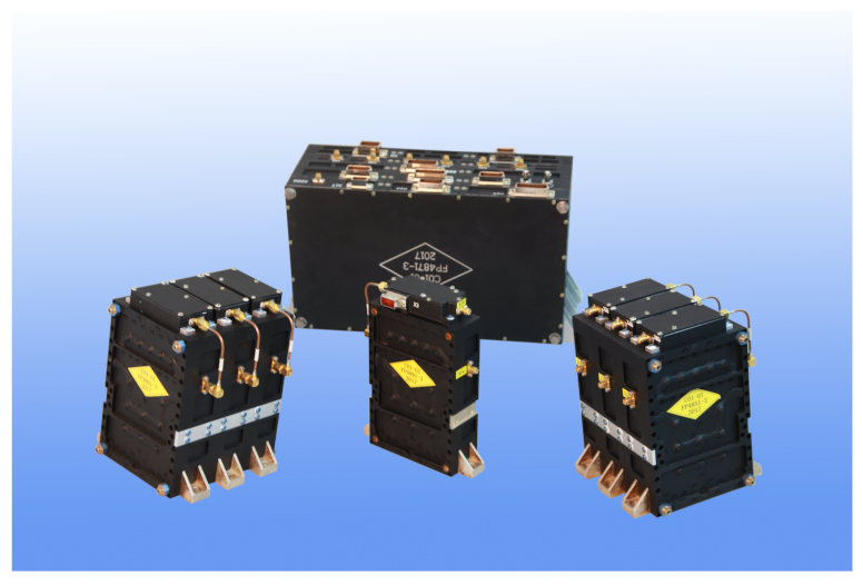
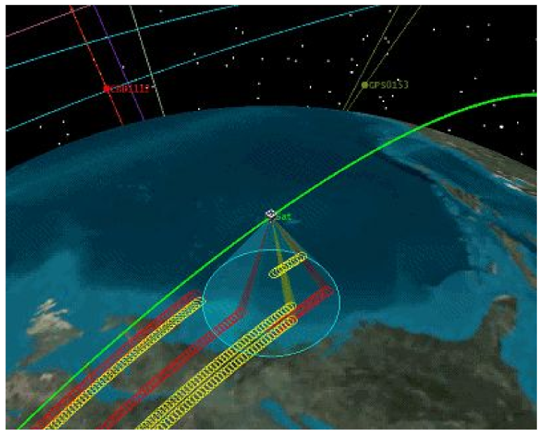
2. Instrument Overview
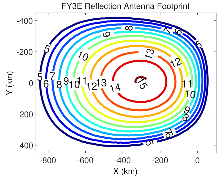
2.1. Non-Uniform Delay-Doppler Mapping
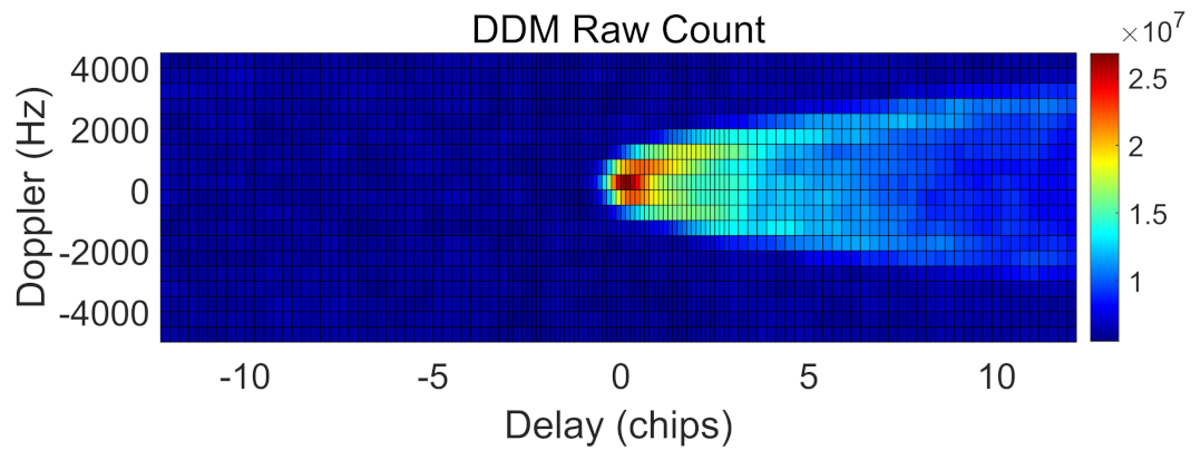
2.2. Raw Sampling Data
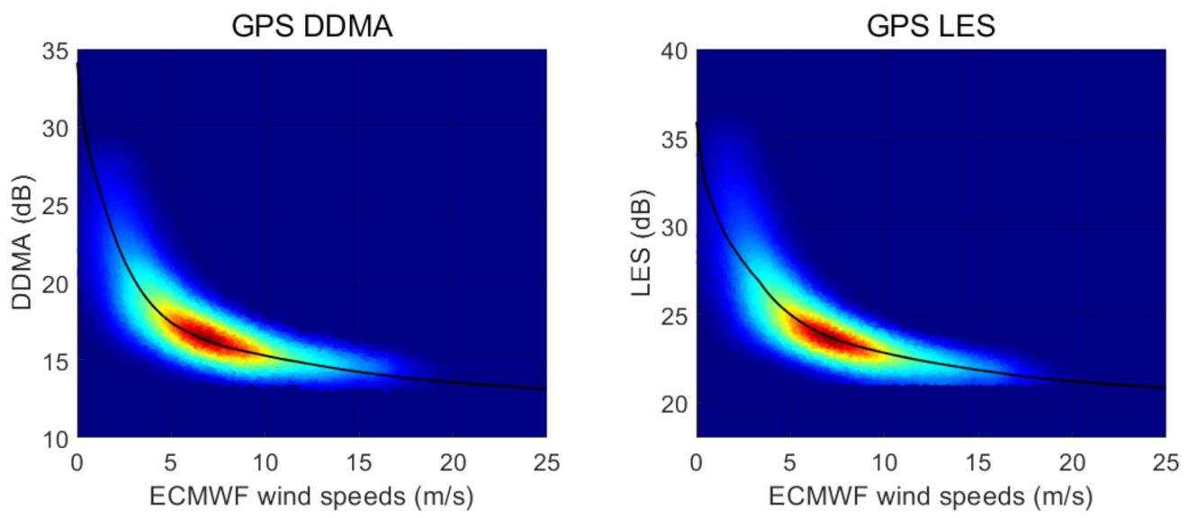
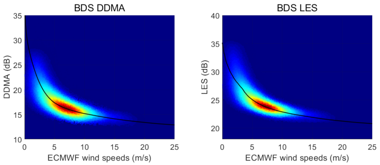
3. L1 Calibration and Level 2 Wind Speed Retrieval
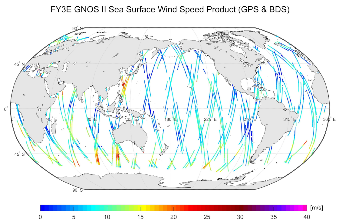
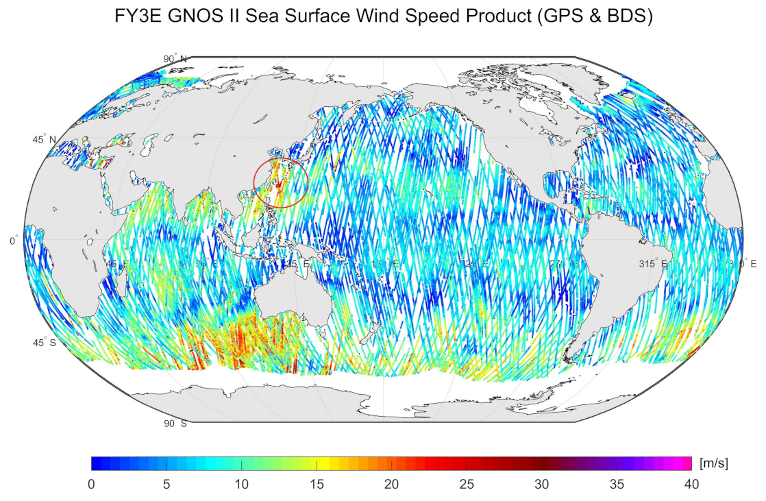
4. Preliminary Validation Results
5. Summary and Future Perspectives
Author Contributions
Funding
Data Availability Statement
Acknowledgments
Conflicts of Interest
References
- Martin-Neira, M. A passive reflectometry and interferometry system (PARIS): Application to ocean altimetry. ESA J. 1993, 17, 331–355. [Google Scholar]
- Clarizia, M.P.; Ruf, C.S. Wind speed retrieval algorithm for the Cyclone Global Navigation Satellite System (CYGNSS) mission. IEEE Trans. Geosci. Remote Sens. 2016, 54, 4419–4432. [Google Scholar] [CrossRef]
- Li, W.; Cardellach, E.; Fabra, F.; Ribó, S.; Rius, A. Assessment of spaceborne GNSS-R ocean altimetry performance using CYGNSS mission raw data. IEEE Trans. Geosci. Remote Sens. 2019, 58, 238–250. [Google Scholar] [CrossRef]
- Wu, X.; Ma, W.; Xia, J.; Bai, W.; Jin, S.; Calabia, A. Spaceborne GNSS-R soil moisture retrieval: Status, development opportunities, and challenges. Remote Sens. 2021, 13, 45. [Google Scholar] [CrossRef]
- Wu, X.; Guo, P.; Sun, Y.; Liang, H.; Zhang, X.; Bai, W. Recent Progress on Vegetation Remote Sensing Using Spaceborne GNSS-Reflectometry. Remote Sens. 2021, 13, 4244. [Google Scholar] [CrossRef]
- Munoz-Martin, J.F.; Perez, A.; Camps, A.; Ribó, S.; Cardellach, E.; Stroeve, J.; Nandan, V.; Itkin, P.; Tonboe, R.; Hendricks, S.; et al. Snow and Ice Thickness Retrievals Using GNSS-R: Preliminary Results of the MOSAiC Experiment. Remote Sens. 2020, 12, 4038. [Google Scholar] [CrossRef]
- Clarizia, M.; Gommenginger, C.; Gleason, S.; Srokosz, M.; Galdi, C.; Di Bisceglie, M. Analysis of GNSS-R delay-Doppler maps from the UK-DMC satellite over the ocean. Geophys. Res. Lett. 2009, 36, L02608. [Google Scholar] [CrossRef] [Green Version]
- Foti, G.; Gommenginger, C.; Jales, P.; Unwin, M.; Shaw, A.; Robertson, C.; Rosello, J. Spaceborne GNSS reflectometry for ocean winds: First results from the UK TechDemoSat-1 mission. Geophys. Res. Lett. 2015, 42, 5435–5441. [Google Scholar] [CrossRef] [Green Version]
- Ruf, C.; Unwin, M.; Dickinson, J.; Rose, R.; Rose, D.; Vincent, M.; Lyons, A. CYGNSS: Enabling the future of hurricane prediction [remote sensing satellites]. IEEE Geosci. Remote Sens. Mag. 2013, 1, 52–67. [Google Scholar] [CrossRef]
- Ruf, C.S.; Chew, C.; Lang, T.; Morris, M.G.; Nave, K.; Ridley, A.; Balasubramaniam, R. A new paradigm in earth environmental monitoring with the cygnss small satellite constellation. Sci. Rep. 2018, 8, 1–13. [Google Scholar] [CrossRef] [PubMed] [Green Version]
- Jing, C.; Niu, X.; Duan, C.; Lu, F.; Di, G.; Yang, X. Sea surface wind speed retrieval from the first Chinese GNSS-R mission: Technique and preliminary results. Remote Sens. 2019, 11, 3013. [Google Scholar] [CrossRef] [Green Version]
- Munoz-Martin, J.F.; Fernandez, L.; Perez, A.; Ruiz-de Azua, J.A.; Park, H.; Camps, A.; Domínguez, B.C.; Pastena, M. In-orbit validation of the FMPL-2 instrument—The GNSS-R and L-band microwave radiometer payload of the FSSCat mission. Remote Sens. 2021, 13, 121. [Google Scholar] [CrossRef]
- Zhang, P.; Hu, X.; Lu, Q.; Zhu, A.; Lin, M.; Sun, L.; Chen, L.; Xu, N. FY-3E: The first operational meteorological satellite mission in an early morning orbit. Adv. Atmos. Sci. 2021, 39, 1–8. [Google Scholar] [CrossRef]
- Sun, Y.; Bai, W.; Liu, C.; Liu, Y.; Du, Q.; Wang, X.; Yang, G.; Liao, M.; Yang, Z.; Zhang, X.; et al. The FengYun-3C radio occultation sounder GNOS: A review of the mission and its early results and science applications. Atmos. Meas. Tech. 2018, 11, 5797–5811. [Google Scholar] [CrossRef] [Green Version]
- Bai, W.; Wang, G.; Sun, Y.; Shi, J.; Yang, G.; Meng, X.; Wang, D.; Du, Q.; Wang, X.; Xia, J.; et al. Application of the Fengyun 3 C GNSS occultation sounder for assessing the global ionospheric response to a magnetic storm event. Atmos. Meas. Tech. 2019, 12, 1483–1493. [Google Scholar] [CrossRef] [Green Version]
- Sun, Y.; Wang, X.; Du, Q.; Bai, W.; Xia, J.; Cai, Y.; Wang, D.; Wu, C.; Meng, X.; Tian, Y.; et al. The Status and Progress of Fengyun-3e GNOS II Mission for GNSS Remote Sensing. In Proceedings of the IGARSS 2019-2019 IEEE International Geoscience and Remote Sensing Symposium, Yokohama, Japan, 28 July–2 August 2019; pp. 5181–5184. [Google Scholar]
- Wang, T.; Ruf, C.S.; Block, B.; McKague, D.S.; Gleason, S. Design and performance of a GPS constellation power monitor system for improved CYGNSS L1B calibration. IEEE J. Sel. Top. Appl. Earth Obs. Remote Sens. 2018, 12, 26–36. [Google Scholar] [CrossRef]
- Xia, J.; Bai, W.; Wu, X.; Sun, Y.; Du, Q.; Wang, X.; Meng, X.; Liu, C.; Zhao, D.; Wan, Y.; et al. Effect of Lhcp Antenna’s Central Beam Direction on DDM’s SNR Around Specular. In Proceedings of the IGARSS 2018-2018 IEEE International Geoscience and Remote Sensing Symposium, Valencia, Spain, 22–27 July 2018; pp. 1067–1070. [Google Scholar]
- Zavorotny, V.U.; Voronovich, A.G. Scattering of GPS signals from the ocean with wind remote sensing application. IEEE Trans. Geosci. Remote Sens. 2000, 38, 951–964. [Google Scholar] [CrossRef] [Green Version]
- Gleason, S.; Ruf, C.S.; Clarizia, M.P.; O’Brien, A.J. Calibration and unwrapping of the normalized scattering cross section for the cyclone global navigation satellite system. IEEE Trans. Geosci. Remote Sens. 2016, 54, 2495–2509. [Google Scholar] [CrossRef]
- Bai, W.; Xia, J.; Zhao, D.; Sun, Y.; Meng, X.; Liu, C.; Du, Q.; Wang, X.; Wang, D.; Wu, D.; et al. GREEPS: An GNSS-R end-to-end performance simulator. In Proceedings of the 2016 IEEE International Geoscience and Remote Sensing Symposium (IGARSS), Beijing, China, 10–15 July 2016; pp. 4831–4834. [Google Scholar]
- Clarizia, M.P.; Ruf, C.S.; Jales, P.; Gommenginger, C. Spaceborne GNSS-R minimum variance wind speed estimator. IEEE Trans. Geosci. Remote Sens. 2014, 52, 6829–6843. [Google Scholar] [CrossRef]
- Hersbach, H.; Bell, B.; Berrisford, P.; Hirahara, S.; Horányi, A.; Muñoz-Sabater, J.; Nicolas, J.; Peubey, C.; Radu, R.; Schepers, D.; et al. The ERA5 global reanalysis. Q. J. R. Meteorol. Soc. 2020, 146, 1999–2049. [Google Scholar] [CrossRef]

Publisher’s Note: MDPI stays neutral with regard to jurisdictional claims in published maps and institutional affiliations. |
© 2022 by the authors. Licensee MDPI, Basel, Switzerland. This article is an open access article distributed under the terms and conditions of the Creative Commons Attribution (CC BY) license (https://creativecommons.org/licenses/by/4.0/).
Share and Cite
Yang, G.; Bai, W.; Wang, J.; Hu, X.; Zhang, P.; Sun, Y.; Xu, N.; Zhai, X.; Xiao, X.; Xia, J.; et al. FY3E GNOS II GNSS Reflectometry: Mission Review and First Results. Remote Sens. 2022, 14, 988. https://doi.org/10.3390/rs14040988
Yang G, Bai W, Wang J, Hu X, Zhang P, Sun Y, Xu N, Zhai X, Xiao X, Xia J, et al. FY3E GNOS II GNSS Reflectometry: Mission Review and First Results. Remote Sensing. 2022; 14(4):988. https://doi.org/10.3390/rs14040988
Chicago/Turabian StyleYang, Guanglin, Weihua Bai, Jinsong Wang, Xiuqing Hu, Peng Zhang, Yueqiang Sun, Na Xu, Xiaochun Zhai, Xianjun Xiao, Junming Xia, and et al. 2022. "FY3E GNOS II GNSS Reflectometry: Mission Review and First Results" Remote Sensing 14, no. 4: 988. https://doi.org/10.3390/rs14040988
APA StyleYang, G., Bai, W., Wang, J., Hu, X., Zhang, P., Sun, Y., Xu, N., Zhai, X., Xiao, X., Xia, J., Huang, F., Yin, C., Du, Q., Wang, X., Cai, Y., Meng, X., Tan, G., Hu, P., & Liu, C. (2022). FY3E GNOS II GNSS Reflectometry: Mission Review and First Results. Remote Sensing, 14(4), 988. https://doi.org/10.3390/rs14040988