Communication

Removal of Ionospheric Effects from Sigma Naught Images of the ALOS/PALSAR-2 Satellite

1
Earth Observation and Geoinformatics Division, National Institute for Space Research (INPE), São José dos Campos 12227-010, SP, Brazil
2
Department of Geography, School of Environment, Education and Development, University of Manchester, Oxford Road, Manchester M13 9PL, UK
*
Author to whom correspondence should be addressed.
Remote Sens. 2022, 14(4), 962; https://doi.org/10.3390/rs14040962
Submission received: 23 January 2022 / Revised: 8 February 2022 / Accepted: 9 February 2022 / Published: 16 February 2022
(This article belongs to the Special Issue Advances in SAR Image Processing and Applications)

Abstract

:
The monitoring of forest degradation in the Amazon through radar remote sensing methodologies has increased intensely in recent years. Synthetic aperture radar (SAR) sensors that operate in L-band have an interesting response for land use and land cover (LULC) as well as for aboveground biomass (AGB). Depending on the magnetic and solar activities and seasonality, plasma bubbles in the ionosphere appear in the equatorial and tropical regions; these factors can cause stripes across SAR images, which disturb the interpretation and the classification. Our article shows a methodology to filter these stripes using Fourier fast transform (FFT), in which a stop-band filter removes this noise. In order to make this possible, we used Environment for Visualizing Images (ENVI), Sentinel Application Platform (SNAP), and Interactive Data Language (IDL). The final filtered scenes were classified by random forest (RF), and the results of this classification showed superior performance compared to the original scenes, showing this methodology can help to recover historic series of L-band images.

Graphical Abstract

1. Introduction

The Amazon has suffered high rates of deforestation in recent decades, resulting from dynamic changes in land use and coverage, which have contributed to the increase in greenhouse gasses, promoting climate change at a regional and global level [1,2,3].
The development of remote sensing methodologies is increasingly necessary and a priority for monitoring this forest degradation promoted by agricultural expansion, urbanization, illegal logging, and extraction of mineral resources [4,5,6,7].
Optical sensor systems, commonly used to map and monitor land use and land cover, are ineffective in tropical regions, and especially in the Amazon, due to frequent cloud cover and adverse atmospheric conditions, which often make it difficult to obtain information from these images during rainy season [8]. In recent years, the use of active sensors (synthetic aperture radar (SAR)) has grown because of its advantages of being able to generate its own energy source, not being influenced by clouds or aerosols, and sensitivity to variations in the forest structure [9,10,11,12,13].
Currently, many orbital SAR sensors are operating at different wavelengths, from 3 to 25 cm, where the greatest penetrations in forest canopies are obtained for the longest wavelengths, such as L-band. The greater penetration of microwaves allows us to understand the different forest strata that make up the forest cover at different stages of ecological succession. This makes it possible to improve the level of thematic characterization of the landscape, enabling the discrimination of different land use types [12,13,14,15,16,17,18].
Among the current operating systems, the Phased Array L-band Synthetic Aperture Radar (PALSAR) sensor aboard the Japanese Space Agency’s (JAXA) Advanced Land Observing Satellite (ALOS) operating in the L-band (1.27 GHz) has been shown to be the most suitable sensor for measurements of signal interaction with the interior of the canopy and, depending on the forest structure, even with the ground surface [19,20].
Due to their longer wavelengths, the ALOS PALSAR-1 and ALOS PALSAR-2 systems (L-band, λ ≅ 20 cm) are more susceptible to ionospheric effects than the shorter wavelength SAR systems (C-band, λ ≅ 5 cm or X-band, λ ≅ 3 cm), which correspond, for example, to the Sentinel-1, RADARSAT Constellation satellites, TerraSAR-X, and CosmoSkyMed.
Previous studies reveled that these scintillation signatures are caused by the turbulent recombination of free electrons in the post-sunset equatorial ionosphere. This can give rise to plumelike irregularity regions with total electron content (TEC) fluctuations that can stretch to over 1000 km along the geomagnetic field lines [21].
These ionospheric disturbances cause a diffractive effect called ionospheric scintillation, which affects the operation of the Global Navigation Satellite System (GNSS) [22,23] as well as causes interference stripes in SAR images, visually perceptible in amplitude or intensity images [24]. This disturbance effect extends distances up to 2000 km [21], degrading the image quality and hindering the classification and identification processing of the studied phenomena [19,25]. Based on 2800 ALOS-PALSAR images (2006 to 2011) acquired at night over South America, it was noticed that 14% of them were contaminated with visible stripes, and in October, 75% of images were contaminated due to ionospheric scintillation [21].
Depending on the solar wind and seasonality (solar activity cycle, ~11 years), ionospheric bubbles appear in the equatorial and tropical regions at latitudes ±20° [19,23,26], being more frequent after sunset and from March to April and September to October [21,26].
This article presents a method to detect and minimize the stripes caused by ionospheric scintillation in the ALOS/PALSAR-2 radar satellite images, through spectral filters in the wavenumber domain, avoiding degradation of resolution and occurrence of artifacts in the classification of images as an intermediate step in the processing chain of Sentinel Application Platform (SNAP) software.

2. Materials and Methods
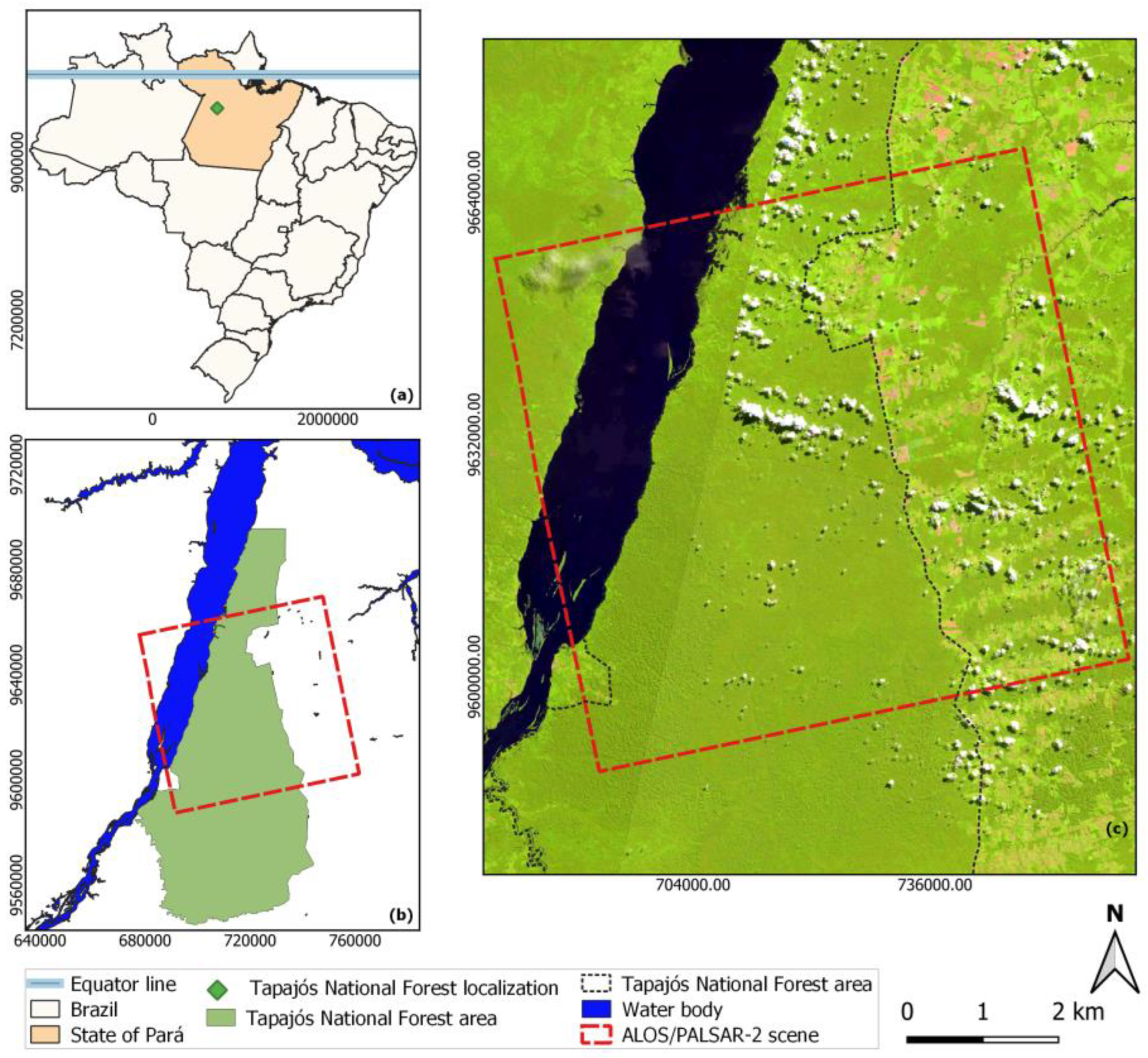
In this section, we describe the test site and the methodological approach proposed in this paper. This approach consists of image processing, classification, and validation.

2.1. Study Area

Our experiment was performed in the Tapajós National Forest (TNF) and its surroundings, located in the Brazilian Amazon rainforest, Pará State, 320 km from the equator (Figure 1). The climate of the region is classified by Köppen as AmW, with an average annual temperature of 25 °C and average relative humidity of 85%. The average annual rainfall is 1909 mm with a dry season between July and November [12].
This site is situated in a relatively flat area with an elevation between 80 and 180 m [12,13]. The vegetation in the TNF is mainly formed by dense and open ombrophylous rainforests. These forests are composed of a continuous canopy of perennial trees with heights between 25 and 30 m, and occasional emergent trees that reach up to 50–60 m in height. The vegetation is also formed by open rainforests, secondary forests, and anthropic areas (crops and pastures), mainly in the surroundings of the national forest [12].

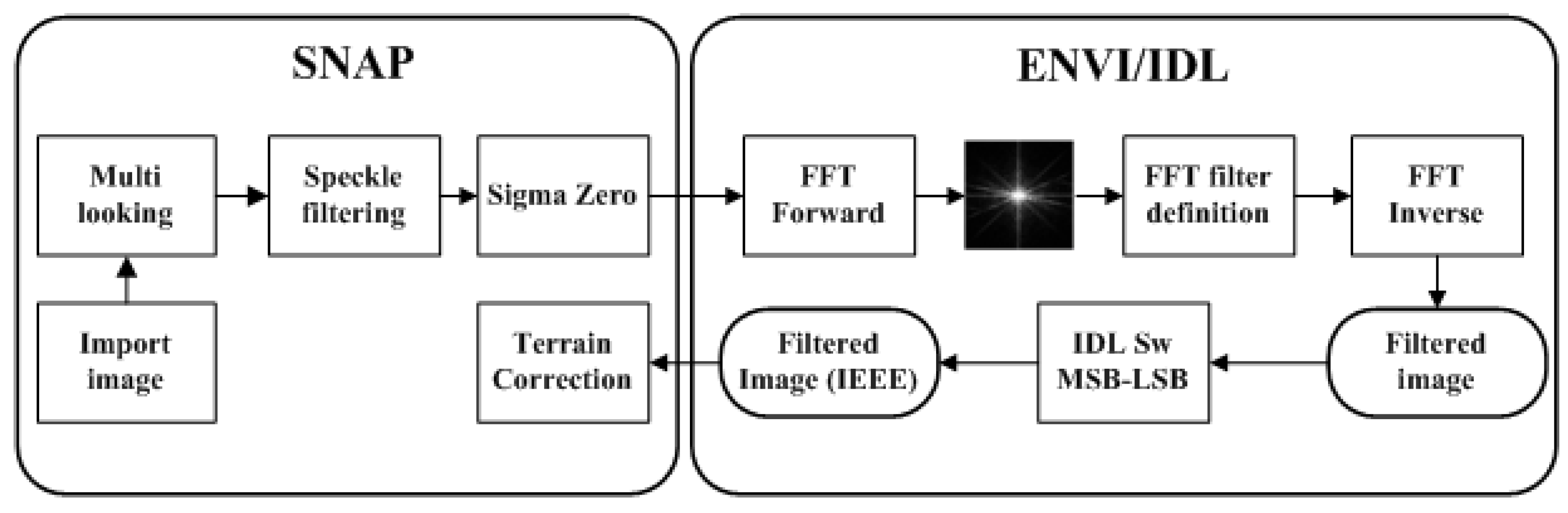
2.2. Methodological Approach
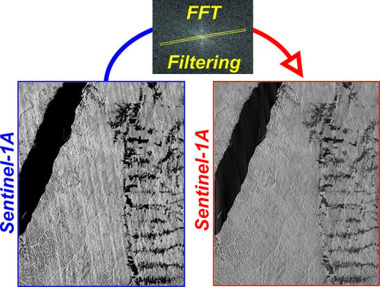
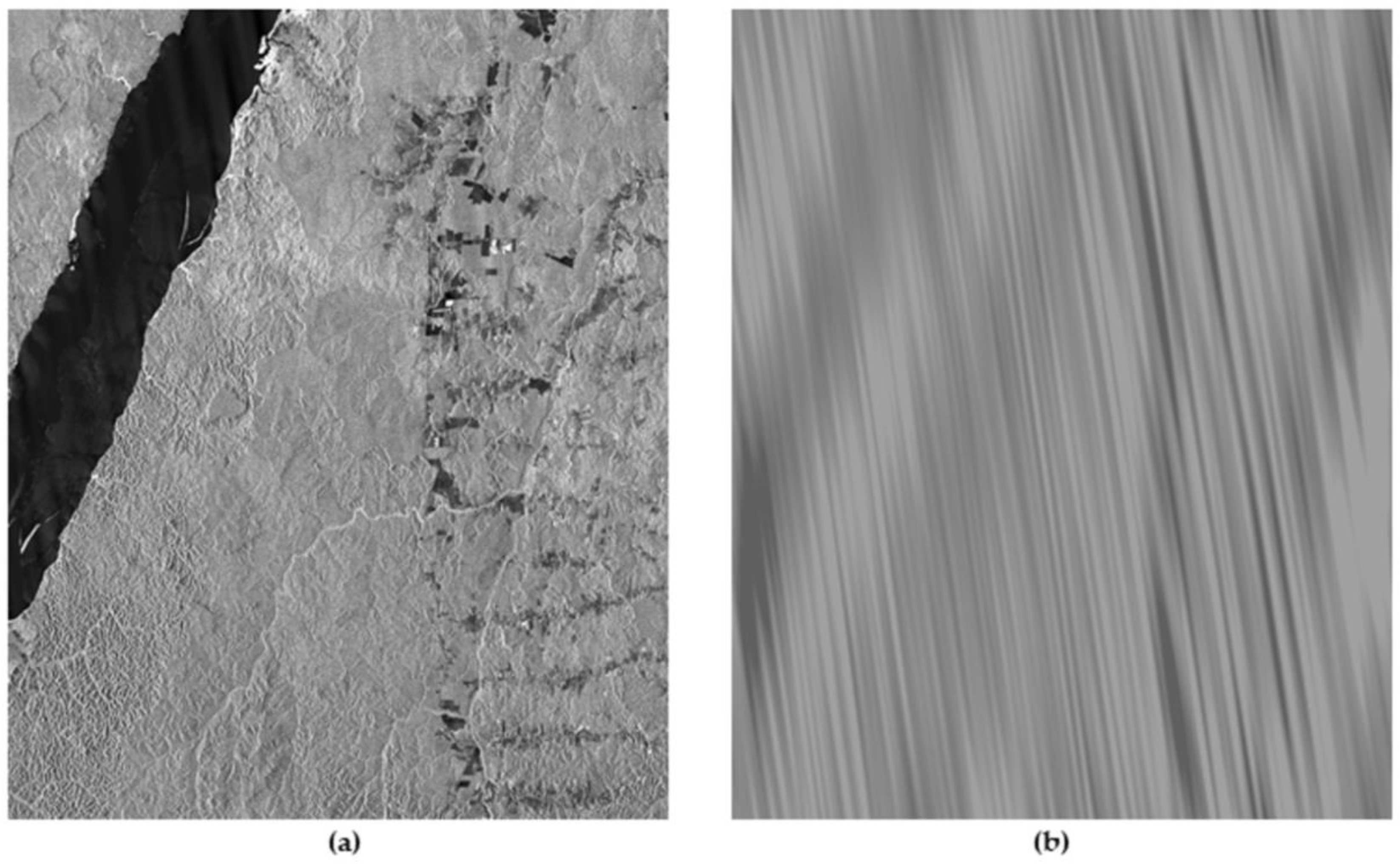
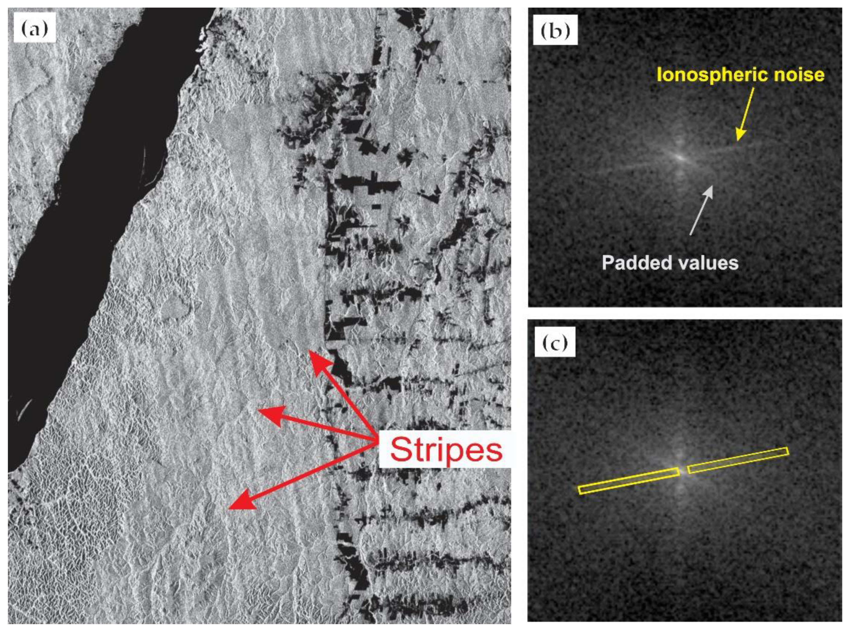
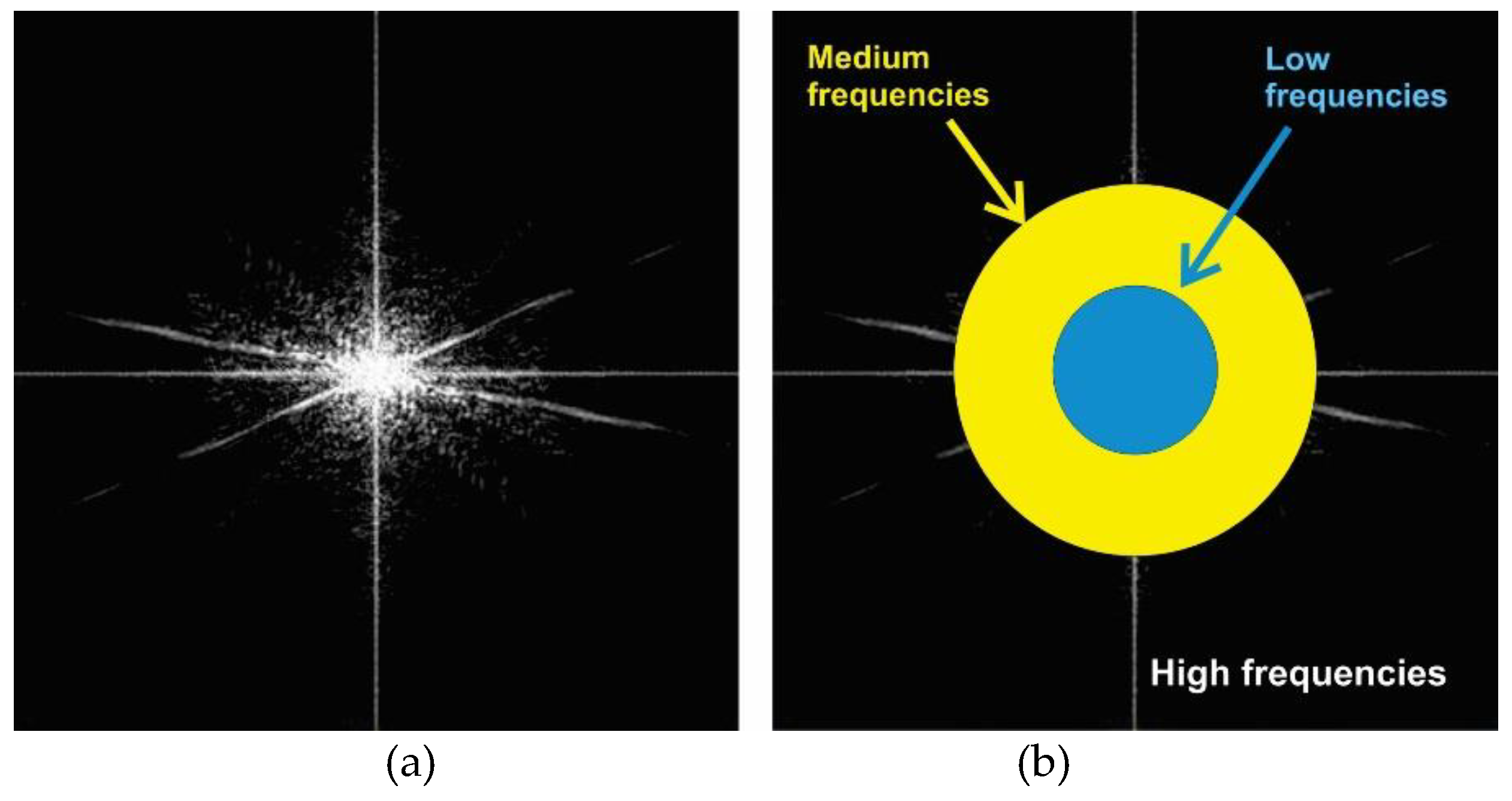
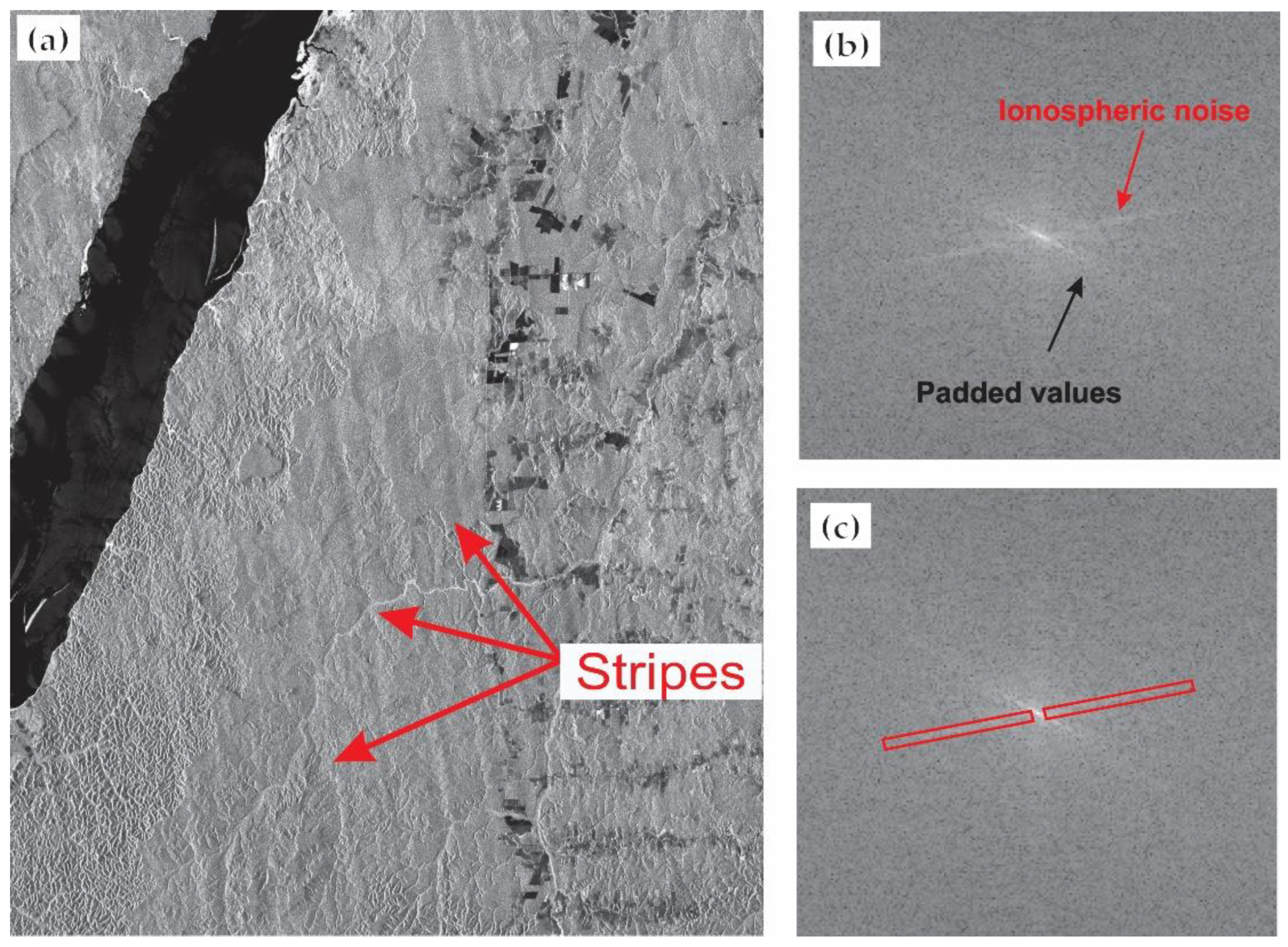
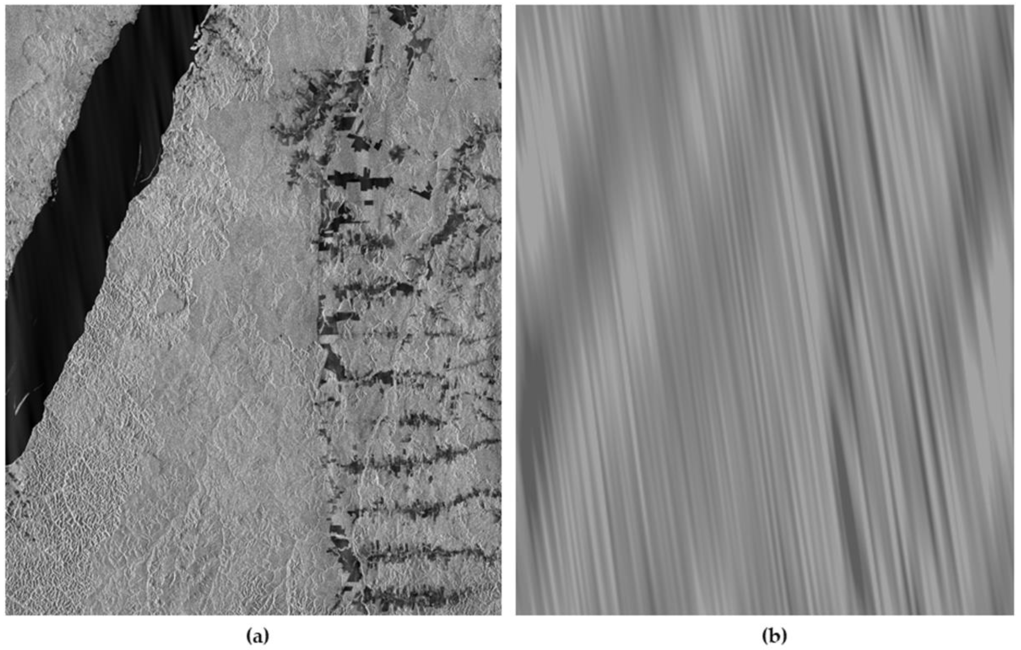
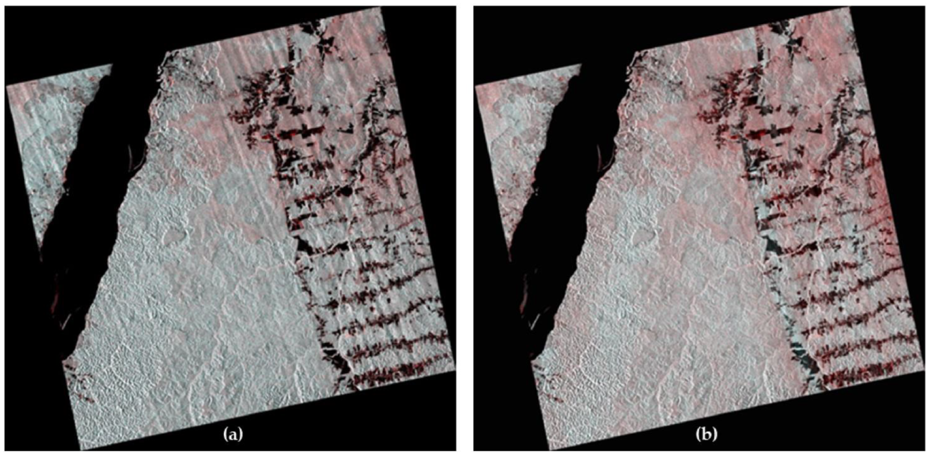
Image filtering can be understood as transformation techniques applied to each pixel of the image, taking into account the magnitude levels of a neighboring region of each pixel of the image. Basically, filtering techniques can be divided into two types: spatial domain and wavenumber domain filtering. Spatial domain filtering refers to the set of pixels that make up an image and a set of values that operate directly on these pixels, which can be expressed as:
g(x,y) = T (f (x,y))
where f (x,y) is the input image, g(x,y) is the processed image, and T is an operator over f, defined over some pixels neighboring the pixel (x,y).
Image filtering in the spatial domain is based on the use of masks. These masks are small matrices and the values of their coefficients determine the objective to be achieved during processing [27], in which this filtering process causes a degradation of the resolution of the final images.
In turn, image processing in the wavenumber domain is usually performed through three basic steps: (a) the image is transformed from the spatial domain to the wavenumber domain (two-dimensional spectrum), using Fourier transform; (b) operations are performed on this new image; (c) the inverse process is performed, in which the image in the wavenumber domain is transformed to the spatial domain (inverse Fourier transform) [27].
The 2-dimensional discrete Fourier transform, which converts image from the spatial domain to the wavenumber domain, can be expressed by:
F ( u , v ) = 1 N M x = 0 M 1 y = 0 N 1 f ( x , y ) e j 2 π ( u x M + v y N )  
where f (x,y) is the image in the spatial domain; F(u,v) is the processed image in the wavenumber domain; and N and M are the size of the image.
The image filtered in the spatial domain can be expressed by:
G(u,v) = F(u,v) H (u,v)
where G(u,v) is the image filtered in the spatial domain; F(u,v) is the original image processed in the wavenumber domain; H(u,v) is the filter function.
In turn, the application of filtering in the two-dimensional spectrum allows great flexibility in removing elements from the image with characteristics that are predominant, so that after removing a characteristic, the inverse Fourier transform is applied, recovering the image and eliminating the unwanted spectrum component but preserving resolution.
The inverse Fourier transform can be expressed by:
f ( x , y ) = u = 0 M 1 v = 0 N 1 G ( u , v ) e   j 2 π ( u x M + v y N )
where f(x,y) is the image in the spatial domain; G(u,v) is the filtered image in the wavenumber domain; N and M are the size of the image.
Figure 2a shows the two-dimensional spectrum of an image, and Figure 2b shows the regions of the two-dimensional spectrum that correspond to the low-, medium-, and high-frequency components of the original image [28,29]. The magnitude of the vector (u,v) gives a frequency, and its direction gives an orientation in the two-dimensional spectrum. The function is a sinusoid with this frequency along the direction, and constant perpendicular to the direction. So, if there is a periodic characteristic in a direction in the original image, its response in the wavenumber domain will be a spectral streak in the orthogonal direction in the two-dimensional spectrum, as illustrated below.
The ALOS PALSAR-1 and ALOS/PALSAR-2 satellites operate in L-band (~20 cm wavelength) and their images acquired in the equatorial zones are susceptible to the effect of ionospheric bubbles, which cause regular patterns in the images, difficult to remove by spatial filtering due to the patterns not being in alignment with the image orientation, which changes as the satellite travels in orbit. By analyzing the images in the wavenumber domain, it is possible to locate the spectral streaks corresponding to these regular patterns, orthogonal to the stripes observed in the original image, and by eliminating the energy from the crests through filtering windows, the noise can be removed. After these procedures, the filtered image can be transformed back to the spatial domain, recovering the backscatter image without the noise.
The data flow diagram in Figure 3 describes the method through which the ALOS/PALSAR satellite image was initially prepared by SNAP-v 8.0 software [12]. This initial processing was responsible for making the pixels regular by the multilooking technique (2 looks for azimuth and 1 look for range), applying the Lee Speckle filter with a 7×7 window size, and finally converting the complex data to sigma naught based on Shimada et al. [30].
For the conversion of sigma naught images to the wavenumber domain using fast Fourier transform (FFT), we used Environment for Visualizing Images (ENVI) and Interactive Data Language (IDL) version 5.4 software.
With the sigma naught images converted in the two-dimensional spectrum, the filtering window in the wavenumber domain was defined (band-stop filter) in the desired spectral streaks. Next, this filtering was performed. Finally, reverse Fourier transform was carried out, generating a new sigma naught image (filtered image) without the pattern caused by the ionospheric bubbles.
As the format of the SNAP images differs from that of ENVI/IDL in the Windows environment, it was necessary to apply a program for compatibility between the Windows data format and the IEEE format, which corresponded to the inversion of the most significant bytes with the least significant ones (MSB–LSB), using the swap_endian function of the IDL language, generating a new image called a filtered image (IEEE).
This new image was geocoded in SNAP using the Range Doppler Terrain Correction option. For this procedure, the SRTM (30 m) was used as the DEM, the DATUM WGS84 was chosen in order to use the same DATUM as the field campaign, carried out for identifying the regions of interest (ROIs); the sampling was nearest neighbor, and the final pixel spacing was 8.24 m.
To evaluate the filtering effect, the images were classified using the random forest (RF) classifier algorithm for land use land cover (LULC) classification. We chose this algorithm because it provides good classification results to discriminate land use and land cover dynamics in rainforests for SAR data [31,32,33]. In this study, we used the Random Forest package available in he R (v.4.01) software [34].
Basically, the RF classifier consists of an ensemble of decision trees, where each tree contributes with just a vote for the assignment of the most frequent class to the input data set, whose final classification result is determined by the most votes of all forest trees. The algorithm uses bagging (bootstrap) and random samples from training sets for tree building with replacement from the original training set [35]. Considering our RF classification, a total of 500 trees were considered. For the RF model training, we used 75% of the samples and 25% for validation, corresponding to 120 well-distributed samples and 39 independent samples, respectively.

3. Results

3.1. Image Processing

For this study, an image from the ALOS/PALSAR-2 satellite, in dual mode (polarizations HH and VV), of the region of the Tapajós National Forest (TNF) with an evident effect of scintillation was used. The description of the ALOS/PALSAR-2 image used is shown in Table 1.
As shown in Figure 4a, the sigma naught image of ALOS/PALSAR-2, polarization HH, has harmonic stripes across it (NNW to SSE direction), being more noticeable in regions with greater anthropization, and less in water areas.
Performing the fast Fourier transform (FFT) of the image, in the 2D image spectrum, we verified the presence of streaks corresponding to the scene details, as well as the noise of ionospheric scintillation (Figure 4b), orthogonal to the stripes’ orientation (WSW to ENE direction), mainly in the low-frequency region of the 2D spectrum. To avoid edge effects in the Fourier transforms, the image was padded in both dimensions, which caused a specific streak in the 2D image spectrum; thus, this signature could be ignored during the processing [26].
In this way, the stop-band filter polygon to remove this streak [25] was defined by visual inspection in the 2D spectral images, using the ENVI Annotation function [36], analyzing the orientation of the streak and its position in the 2D spectrum. So, the entire streak was covered by this polygon and the stop-band filter was able to remove the scintillation noise streak.
Following removal of scintillation noise by the stop-band filter, the inverse FFT transformation was performed to restore the sigma naught image (HH) filtered (Figure 5a).
In turn, to confirm if the polygon of stop-band filter was in the correct position on the scintillation noise streak of the ALOS/PALSAR-2 image (Figure 4b), a pass-band filter using the same polygon of the stop-band was applied on the original image to allow isolating the scintillation noise. We noticed that the noise extracted (Figure 5b) had the same orientation as the stripes observed in the original image (Figure 4a), confirming that the polygon was positioned in the correct streak.
Figure 6a shows the sigma naught image of ALOS/PALSAR-2 for the HV polarization, with a similar ionospheric harmonic stripes effect observed in HH polarization. The streak of ionospheric scintillation noise, orthogonal to the stripes’ orientation, is shown in the 2D image spectrum in Figure 6b, as well as the padded values streak. Similar to the HH image, the streaks of the scintillation concentrated on the low frequencies (Figure 6b), which were responsible for the oscillation image values.
The sigma naught L-band image, HV polarization, showed stripes with NNW to SSE direction, similar to the HH image. So, the same filtering procedure performed for HH polarization image was applied to the HV image. The stop-band filtering was defined by visual analysis in order to cover the entire streak orthogonal to the stripes’ orientation (WSW to ENE direction) and disregarding the padded streak. The result of the processing is shown in Figure 7a.
In order to verify if the polygon of the stop-band filter was positioned in the correct streak (noise streak), the same polygon was applied for the pass-band filter. Figure 7b shows the result of pass-band filtering, where the noise stripes have the same orientation as the original image stripes (Figure 6a), showing that the polygon of filtering was positioned on the correct streak, and it was able to extract the scintillation noise stripes.
After noise removal processing of the images with HH and HV polarizations in ENVI, the IDL routine described in the methodology was used to allow importing them into SNAP for geocoding (range Doppler terrain correction).
The original and filtered images (HH and HV) with terrain correction were recombined using the RStudio environment, with the HV composition for the red channel and HH for the green channel; the blue channel was not filled (Figure 8). These compositions were necessary for the classification process using random forest.

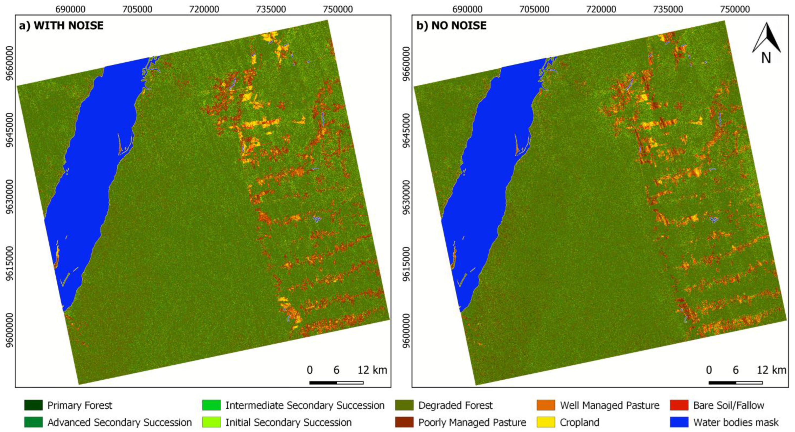
3.2. Random Forest Classification

The classification result for scenes with scintillation noise and with scintillation noise removal are shown in Figure 9. A body water mask was used in order to not confuse the LULC classification and thus obtain the best results. The regions of interest (ROIs) for the classification were based on the data collected during the field work in the TNF.
For the classification performed, the classes Primary Forest (PF), Advanced Secondary Succession (SS3), Intermediate Secondary Succession (SS2), Initial Secondary Succession (SS1), Poorly Managed Pasture (PP), Well Man-aged Pasture (WP), Cropland (CR), Degraded Forest (DF), and Bare Soil/Fallow (BS) were analyzed based on the field surveying carried out at the test site in September 2016, that categorized these classes of landscape [12]. Table 2 describes the LULC classes analyzed.
Comparing the performance tables of the scenes’ classifications for the filtered and non-filtered images, some LULC classes were changed, as in the case of PP class improvement as well as the DF, SS2, and WP classes. This can also be seen by the Kappa index, which was higher for the filtered images (0.51), as presented in the Table 3 footer, than for the original images (0.48) in the Table 4 footer. The overall accuracy (OA) of RF classification showed a better value for the filtered scenes (0.6) than the original scenes (0.57).

4. Discussion

Some studies reported that scintillation noise causes disturbance in polarimetric images [21,37]. This was also noticed in our experiment, lowering RF classification performance for the original scenes. Our classification performance showed that Kappa and the OA indexes were improved when noise removal was performed, which presented similar classification results to those obtained using L-band images without scintillation effect by [14] using JERS-1 data, and by [38] using ALOS PALSAR, showing that the methodology used in this study can improve data quality, especially for LULC applications.
A little noise from the remaining scintillation in the Tapajós River region was perceived in the HH polarization image, since this polarization has a greater response to the surface of water bodies due to currents and winds. This behavior was also observed by [25]. For the HV polarization image, this scintillation effect was not noticed in the filtered images.
The positioning of the stop-band filtering windows, by visual analysis, required some tests until reaching the correct spectral streak (Figure 4b and Figure 6b), corresponding to ionospheric scintillation, avoiding the target’s characteristics removal. This outcome was also observed by [25]. Based on this evidence, it is important to highlight that an automated or semi-automated process could be applied to make the search faster.
Due to fact that all processing was carried out in the Windows environment, the IDL routine was necessary to be applied (bytes inversion); if the Linux environment were to be used, the IDL routine step would not be necessary, which would simplify the processing. If the SNAP program incorporates FFT filtering tools in the future, the entire processing chain could be carried out simultaneously, simplifying the execution.

5. Conclusions

The method proposed here was shown to be effective in removing the scintillation noise from sigma naught ALOS/PALSAR-2 images, improving the classification of different targets of interest. This methodology can also be applied to data from other L-band sensors, such as the SAOCOM satellite, over tropical zones, which can be helpful for studies of historic series of L-band images.
The location of the stop-band filtering in the 2D spectrum band of the images demands certain effort as well as the definition of the dimensions of the polygon of the filtering window to cover the spectral streak of the noise. In this way, a need remains for the development of techniques that can automate this process, avoiding any filtering mistakes.
In case the stripes of the image are perfectly aligned with the image acquisition orientation, it will be difficult to locate the streak of the noise in the 2D spectrum. Therefore, it would be better, in this case, to average image columns to determine the correction function.
The processing was carried out using ENVI software, a programming routine in IDL, and SNAP software; other environments and languages can also be used, such as Python or C++, for instance, but they will demand a greater effort in the development of programming routines.
Although the Kappa and OA values were not very high after the proposed processing, there was a substantial visual improvement in the images, as shown in Figure 8b, which greatly facilitates their interpretation when the noise effect is removed.
In this study, we used sigma naught ALOS PALSAR-2 images, but the same methodology may also be applied to amplitude or intensity images; in turn, complex images will require more studies to determine the effects of scintillation noise in the phase data.
In case of flexibility in the acquisition scheduling of L-band data for tropical regions close to the equator (±20°), we suggest avoiding the periods from March to April and September to October in order to prevent expressive effect of atmospheric scintillation, especially after sunset, when the phenomenon is more intense.

Author Contributions

F.F.G. was in charge of SAR processing; F.F.G., P.d.C.B. and N.C.W. carried out the analysis of results and wrote the manuscript. All authors have read and agreed to the published version of the manuscript.

Funding

This research received no external funding.

Institutional Review Board Statement

Not applicable.

Informed Consent Statement

Not applicable.

Data Availability Statement

ALOS/PALSAR-2 data was provided by JAXA Japan Aerospace Exploration Agency (JAXA), under ALOS Research Announcement (Process 1090).

Acknowledgments

The authors are grateful for the support of Edson E. Sano (Embrapa Cerrados) and the Japan Aerospace Exploration Agency (JAXA), under ALOS Research Announcement (Process 1090), which provided ALOS/PALSAR-2 data.

Conflicts of Interest

The authors declare no conflict of interest.

Abbreviations

SARSynthetic Aperture Radar
LULCLand Use Land Cover
FFTFourier Fast Transform
AGBAboveground Biomass
OAOverall Accuracy
IDLInteractive Data Language
PALSARPhased Array L-band Synthetic Aperture Radar
ALOSAdvanced Land Observing Satellite
TNFTapajós National Forest
GNSSGlobal Navigation Satellite System
RFRandom Forest Classifier
SNAPSentinel Application Platform
ENVIEnvironment for Visualizing Images

References

  1. Pielke, R.A. Land use and climate change. Science 2005, 310, 1625–1626. [Google Scholar] [CrossRef] [PubMed] [Green Version]
  2. Foley, J.A.; Defries, R.; Asner, G.P.; Barford, C.; Bonan, G.; Carpenter, S.R.; Chapin, F.S.; Coe, M.T.; Daily, G.C.; Gibbs, H.K.; et al. Global consequences of land use. Science 2005, 309, 570–574. [Google Scholar] [CrossRef] [PubMed] [Green Version]
  3. Junior, C.H.S.; Pessôa, A.C.; Carvalho, N.S.; Reis, J.B.; Anderson, L.O.; Aragão, L.E. The Brazilian Amazon deforestation rate in 2020 is the greatest of the decade. Nat. Ecol. Evol. 2021, 5, 144–145. [Google Scholar] [CrossRef] [PubMed]
  4. Lemos, A.L.F.; Silva, J.A. Desmatamento na Amazônia Legal: Evolução, causas, monitoramento e possibilidades de mitigação através do Fundo Amazônia. Revista Floresta e Ambiente 2011, 8, 98–108. [Google Scholar] [CrossRef]
  5. Matricardi, E.A.T.; Skole, D.L.; Costa, O.B.; Pedlowski, M.A.; Samek, J.H.; Miguel, E.P. Long-Term Forest Degradation Surpasses Deforestation in the Brazilian Amazon. Science 2020, 369, 1378–1382. [Google Scholar] [CrossRef]
  6. Qin, Y.; Xiao, X.; Wigneron, J.P.; Ciais, P.; Brandt, M.; Fan, L.; Li, X.; Crowell, S.; Wu, X.; Doughty, R.; et al. Carbon Loss from Forest Degradation Exceeds that from Deforestation in the Brazilian Amazon. Nat. Clim. Change 2021, 11, 442–448. [Google Scholar] [CrossRef]
  7. Kuck, T.N.; Sano, E.E.; Bispo, P.D.C.; Shiguemori, E.H.; Silva Filho, P.F.F.; Matricardi, E.A.T. A Comparative Assessment of Machine-Learning Techniques for Forest Degradation Caused by Selective Logging in an Amazon Region Using Multitemporal X-Band SAR Images. Remote Sens. 2021, 13, 3341. [Google Scholar] [CrossRef]
  8. Asner, G.P. Cloud cover in Landsat observations of the Brazilian Amazon. Int. J. Remote Sens. 2001, 22, 3855–3862. [Google Scholar] [CrossRef]
  9. Kasischke, E.S.; Melack, J.M.; Dobson, M.C. The use of imaging radars for ecological applications: A review. Remote Sens. Environ. 1997, 57, 141–156. [Google Scholar] [CrossRef]
  10. Henderson, F.M.; Lewis, A.J. Manual of Remote Sensing: Principles and Applications of Imaging Radars, 3rd ed.; John Wiley & Sons: New York, NY, USA, 1998; 866p. [Google Scholar]
  11. Santos, J.R.; Freitas, C.C.; Araújo, L.S.; Dutra, L.V.; Mura, J.C.; Gama, F.F.; Soler, L.S.; Sant’anna, S.J.S. Airborne P-band SAR applied to the above ground biomass studies in the Brazilian tropical rainforest. Remote Sens. Environ. 2003, 87, 482–493. [Google Scholar] [CrossRef]
  12. Wiederkehr, N.C.; Gama, F.F.; Castro, P.B.N.; Bispo, P.d.C.; Balzter, H.; Sano, E.E.; Liesenberg, V.; Santos, J.R.; Mura, J.C. Discriminating Forest Successional Stages, Forest Degradation, and Land use in Central Amazon Using ALOS/PALSAR-2 Full-Polarimetric Data. Remote Sens. 2020, 12, 3512. [Google Scholar] [CrossRef]
  13. Bispo, P.C.; Santos, J.R.; Valeriano, M.M.; Touzi, R.; Seifert, F.M. Integration of polarimetric PALSAR attributes and local geomorphometric variables derived from SRTM for forest biomass modeling in central Amazonia. Can. J. Remote Sens. 2014, 40, 26–42. [Google Scholar] [CrossRef]
  14. Dutra, L.V.; Scofield, G.B.; Neta, S.A.R.; Negri, R.G.; Freitas, C.C.; Andrade, D. Land cover classification in Amazon using Alos Palsar Full Polarimetric Data. In Simpósio Brasileiro de Sensoriamento Remoto; INPE: São José dos Campos, Brasil, 2009; Volume 1, pp. 7259–7264. ISBN 978-85-17-00044-7. (INPE-15865-PRE/10475). Available online: http://urlib.net/dpi.inpe.br/sbsr@80/2008/11.17.18.24 (accessed on 18 December 2021).
  15. Li, G.; Lu, D.; Moran, E.; Dutra, L.; Batistella, M. A comparative analysis of ALOS PALSAR L-band and RADARSAT-2 C-band data for land-cover classification in a tropical moist region. ISPRS J. Photogramm. Remote Sens. 2012, 70, 26–38. [Google Scholar] [CrossRef] [Green Version]
  16. Negri, R.; Dutra, L.; Freitas, C.D.C.; Lu, D. Exploring the Capability of ALOS PALSAR L-Band Fully Polarimetric Data for Land Cover Classification in Tropical Environments. IEEE J. Sel. Top. Appl. Earth Obs. Remote Sens. 2016, 9, 5369–5384. [Google Scholar] [CrossRef]
  17. Pôssa, E.M. Discriminação de uso e cobertura da terra na região amazônica a partir de informação polarimétrica ALOS/PALSAR e coerência interferométrica da missão TANDEM-X. Master’s Thesis, Instituto Nacional de Pesquisas Espaciais, São José dos Campos, Brasil, 2016. Available online: http://urlib.net/8JMKD3MGP3W34P/3L65BH8 (accessed on 16 December 2021).
  18. Costa, J.D.S.; Liesenberg, V.; Schimalski, M.B.; de Sousa, R.V.; Biffi, L.J.; Gomes, A.R.; Neto, S.L.R.; Mitishita, E.; Bispo, P.D.C. Benefits of Combining ALOS/PALSAR-2 and Sentinel-2A Data in the Classification of Land Cover Classes in the Santa Catarina Southern Plateau. Remote Sens. 2021, 13, 229. [Google Scholar] [CrossRef]
  19. Shimada, M.; Muraki, Y.; Otsuka, Y. Discovery of Anoumoulous Stripes Over the Amazon by the PALSAR onboard ALOS Satellite. In Proceedings of the IEEE International Geoscience and Remote Sensing Symposium (IGARSS), Boston, MA, USA, 7–11 July 2008; pp. II-387–II-390. [Google Scholar]
  20. Jensen, J.R. Sensoriamento Remoto do ambiente: Uma Perspectiva em Recursos terrestres, 2nd ed.; Epiphanio, T.J.C.N., Formaggio, A.R., Santos, A.R., De Almeida, C.M., Theodor Rudorff, B.R., Galvão, L.S., Eds.; Parêntese: São José dos CamposParêntese, Brazil, 2009; 625p. [Google Scholar]
  21. Meyer, F.J.; Chotoo, K.; Chotoo, S.D.; Huxtable, B.D.; Carrano, C.S. The Influence of Equatorial Scintillation on L-Band SAR Image Quality and Phase. IEEE Trans. Geosci. Remote Sens. 2015, 54, 869–880. [Google Scholar] [CrossRef]
  22. Paulino, I.; Medeiros, A.F.; Buriti, R.A.; Takahashi, H.; Sobral, J.H.A.; Gobbi, D. Plasma bubble zonal drift characteristics observed by airglow images over Brazilian tropical region. Revista Brasileira de Geofísica 2011, 29, 239–246. [Google Scholar] [CrossRef]
  23. Mendonça, M.A.M.; Monico, J.F.G.; Motoki, G.M. Efeitos da cintilação ionosférica na agricultura de precisão: Um estudo de caso. In Proceedings of the II Simpósio Brasileiro de Geomática e V Colóquio Brasileiro de Ciências Geodésicas, Presidente Prudente, Brasil, 24–27 July 2012; 2012; Volume 1, pp. 262–267. [Google Scholar]
  24. Sato, H.; Kim, J.S.; Wrasse, C.M.; Souza, J.R. Sounding the Origin Of L-Band SAR Stripes in the Equatorial Ionosphere: Coordinated Observation of Alos-2 And Air Glow Imager. In Proceedings of the IEEE International Geoscience and Remote Sensing Symposium (IGARSS), Yokohama, Japan, 28 July–2 August 2019; pp. 7702–7705. [Google Scholar]
  25. Roth, A.P.; Huxtable, B.D.; Chotoo, K.; Chotoo, S.D.; Caton, R.G. Detection and mitigation of ionospheric stripes in PALSAR data. In Proceedings of the IEEE International Geoscience and Remote Sensing Symposium, Munich, Germany, 22–27 July 2012; pp. 1621–1624. [Google Scholar] [CrossRef]
  26. Abdu, M.A.; Batista, I.S.; Takahashi, H.; MacDougall, J.; Sobral, J.H.; De Medeiros, A.; Trivedi, N.B. Magnetospheric disturbance induced equatorial plasma bubble development and dynamics: A case study in Brazilian sector. J. Geophys. Res. Earth Surf. 2003, 108, 13. [Google Scholar] [CrossRef] [Green Version]
  27. Gonzalez, R.C.; Woods, R.E. Digital Image Processing, 4th ed.; Pearson: New York, NY, USA, 2018; 1192p. [Google Scholar]
  28. Mather, P.M. Computer Processing of Remotely-Sensed Images; John Wiley & Sons: Chichester, UK, 1993. [Google Scholar]
  29. Richards, J.A. Remote sensing Digital Image Analysis; Spinger: Berlin/Heidelberg, Germany, 1995. [Google Scholar]
  30. Shimada, M.; Isoguchi, O.; Tadono, T.; Isono, K. PALSAR Radiometric and geometric calibration. IEEE Trans. Geosci. Remote Sens. 2009, 7, 3915–3932. [Google Scholar] [CrossRef]
  31. Hagensieker, R.; Waske, B. Evaluation of multi-frequency SAR images for tropical land cover mapping. Remote Sens. 2018, 10, 257. [Google Scholar] [CrossRef] [Green Version]
  32. Pavanelli, J.A.P.; Santos, J.R.; Galvão, L.S.; Xaud, M.; Xaud, H.A.M. PALSAR-2/ALOS-2 and OLI/LANDSAT-8 data integration for land use and land cover mapping in northern Brazilian Amazon. Boletim de Ciências Geodésicas 2018, 24, 250–269. [Google Scholar] [CrossRef]
  33. Diniz, J.M.F.S.; Gama, F.F.; Adami, M. Evaluation of polarimetry and interferometry of sentinel-1A SAR data for land use and land cover of the Brazilian Amazon region. Geocarto Int. 2020, v. 35, 1–19. [Google Scholar] [CrossRef]
  34. R Core Team. R: A Language and Environment for Statistical Computing; R Foundation for Statistical Computing: Vienna, Austria, 2020. Available online: https://www.R-project.org/ (accessed on 1 February 2022).
  35. Breiman, L. Random Forests. Mach. Learn. 2001, 45, 5–32. [Google Scholar] [CrossRef] [Green Version]
  36. ENVI. Using ENVI. Available online: https://www.l3harrisgeospatial.com/docs/routines-136.html (accessed on 5 February 2022).
  37. Belcher, D.P.; Cannon, P.S. Amplitude scintillation effects on SAR. IET Radar Sonar Navig. 2014, 8, 658–666. [Google Scholar] [CrossRef]
  38. Camargo, F.F.; Sano, E.E.; Almeida, C.M.; Mura, J.C.; Almeida, T. A Comparative Assessment of Machine-Learning Techniques for Land Use and Land Cover Classification of the Brazilian Tropical Savanna Using ALOS-2/PALSAR-2 Polarimetric Images. Remote Sens. 2019, 11, 1600. [Google Scholar] [CrossRef] [Green Version]
Figure 1. (a) Study area location and the equator line (blue line); (b) Tapajós National Forest in Pará State/Brazil; (c) ALOS/PALSAR-2 footprint and Landsat-8 image as background.
Remotesensing 14 00962 g001
Figure 2. (a) Two-dimensional spectrum of an image; (b) location of the low-, medium-, and high-frequency components of the two-dimensional spectrum.
Remotesensing 14 00962 g002
Figure 3. Processing steps.
Remotesensing 14 00962 g003
Figure 4. (a) ALOS/PALSAR-2 scene, HH polarization, image with stripes; (b) 2D image spectrum image; (c) 2D image spectrum with the corresponding stop-band filtering window in red.
Remotesensing 14 00962 g004
Figure 5. (a) ALOS/PALSAR-2 scene, HH polarization, after stripes removed; (b) stripes image obtained by the pass-band filtering and inverse FFT.
Remotesensing 14 00962 g005
Figure 6. (a) ALOS/PALSAR-2 scene, HV polarization, image with stripes; (b) 2D image spectrum image; (c) 2D image spectrum with the corresponding stop-band filtering window in yellow.
Remotesensing 14 00962 g006
Figure 7. (a) ALOS/PALSAR-2 scene, HV polarization, with scintillation noise removed; (b) scintillation noise extracted by pass-band filtering and inverse FFT.
Remotesensing 14 00962 g007
Figure 8. Composition of the image where the red channel corresponds to HV polarization and the green channel to HH polarization for: (a) without and (b) with noise removal.
Remotesensing 14 00962 g008
Figure 9. Random forest classification results for the scenes: (a) with scintillation noise and (b) with scintillation noise removal.
Remotesensing 14 00962 g009
Table 1. SAR image used.
ImageOrbitDatePolarization
ALOS2187487120-171112Ascending12 November 2017HH
HV
Table 2. Land use and land cover classes.
ClassDescriptionClassDescription
DFForests that suffered a slight loss of density due to indiscriminate logging and/or burning activitiesCRAgricultural crops throughout the phenological development phase
PFForests without anthropogenic changeBSTemporary agricultural rest areas between growing seasons
SS3Natural regeneration over 15 yearsWPWell-managed pastures with few invasive species
SS2Natural regeneration from 5 to 15 yearsPPPastures with the presence of species shrub weeds, babassu and/or inajá
SS1Natural regeneration under 5 years----
Table 3. Performance of the RF algorithm for the scenes after filtering.
ClassesPFSS3SS2SS1PPWPCRDFBS
PF010000020
SS3122000050
SS20310431280
SS1303111226100
PP001022121331150
WP00021754203
CR02135117012
DF12141110705980
BS0000114024
*Kappa: 0.51; overall accuracy (OA): 0.60
Table 4. Performance of the RF algorithm for the original scenes without filtering.
ClassesPFSS3SS2SS1PPWPCRDFBS
PF111000010
SS3161000050
SS2105131060
SS15431851560
PP201218107371346
WP00113148903
CR105112167008
DF911129400940
BS0000114022
*Kappa: 0.48; overall accuracy (OA): 0.57
Publisher’s Note: MDPI stays neutral with regard to jurisdictional claims in published maps and institutional affiliations.

