Assessment of Nighttime Cloud Cover Products from MODIS and Himawari-8 Data with Ground-Based Camera Observations

Abstract

Comparing cloud cover (CC) products from different satellites with the same ground-based CC dataset provides information on the similarities or differences of values among satellite products. For this reason, 42-month CC products from Moderate Resolution Imaging Spectrometer’s (MODIS) Collection 6.1 daily cloud cover products (MOD06_L2, MYD06_L2, MOD08_D3, and MYD08_D3) and Himawari-8 are compared with the ground-based camera datasets. The comparison shows that CC from MODIS differs from ground measurement CC by as much as 57% over Chiba, Japan, when low CC is observed by the camera. This indicates MODIS’s ability to capture high-level clouds that are not effectively seen from the ground. When the camera detects high CC, an indication of the presence of low-level clouds, CC from MODIS is relatively higher than the CC from the camera. In the case of Himawari-8 data, when the camera observes low CC, this difference is around 0.7%. This result indicates that high-level clouds are not effectively observed, but the Himawari-8 data correlates well with camera observations. When the camera observes high CC, Himawari-8-derived CC is lower by around 10% than CC from the camera. These results show the potential of continuous observations of nighttime clouds using the camera to provide a dataset that can be used for intercomparison among nighttime satellite CC products.

1. Introduction

Atmospheric clouds are composed of minute liquid droplets and ice crystals in the atmosphere. When electromagnetic radiation from the Sun and Earth interacts with clouds, this radiation is either absorbed, reradiated, scattered, or reflected. As a result, clouds can enhance the Earth’s atmospheric cooling or warming effects. The extent of cloud cover (CC) is one of the parameters that regulate the amount of net radiative flux in the atmosphere [1,2]. Cloud type and albedo also control the net radiation balance in the atmosphere [3]. Radiative feedback from clouds has high uncertainties, particularly due to the uncertainty of the impact of low-level clouds on warming. Currently, the resulting positive feedback is still variable among model simulations and not properly constrained by observations [4,5,6]. Thus, there is a need for continuous observations from both the ground and space. At nighttime, longwave effects dominate since clouds reradiate longwave radiation from the ground. Low-level clouds such as cumulus, cumulonimbus, and stratocumulus are easily observed by ground-based image sensors such as cameras. On the other hand, satellites cannot efficiently detect low-level clouds when ground and cloud-top temperatures are similar. In terms of the radiative effects, previous studies have shown that these low-level clouds have a higher longwave effect than mid-level clouds (e.g., cirrocumulus) [7,8].

Satellites are common sources of CC data, which yields CC products valuable for deducing cloud optical properties and modeling cloud radiative transfer [9,10,11,12]. To minimize the errors in measuring net radiative effects in the atmosphere, the dataset from continuously operated ground-based cameras can aid in ground-truthing satellite data.

Polar-orbiting satellites can provide CC data over an area during an overpass. For the Moderate Resolution Imaging Spectroradiometer (MODIS) onboard Terra/Aqua satellites, data are obtained around 10:30 and 22:30 (for Terra) and around 13:30 and 01:30 (for Aqua) local time. Much more frequent data are available from geosynchronous satellites. Himawari-8, for instance, provides a full disk scene every 10 min [13]. Such data with a finer temporal resolution enables studying and tracking clouds’ dynamics and behavior. Compared to polar-orbiting satellites, the volume of data from geosynchronous satellites can be enormous, and the analysis of these datasets is computationally intensive. Still, the data provides more precise information on the temporal changes of CC over an area and the capability of elucidating the seasonal characterization of CC values, and hence, the radiative effects of clouds in different months.

Based on years of satellite observations of clouds, previous studies have reported an increase and a decrease in global CC from 1983 to 2001 [14] and a decrease in CC between 40° S and 40° N in the frame of the International Satellite Cloud Climatology Project (ISCCP) [15]. In terms of cloud occurrence, a previous investigation showed that the global annual mean cloud amount is around 63%, with the oceans having 23% more CC than land [16]. Cloud climate data records from 1984–2009 also show good agreement on global cloud amounts and a weak negative trend of 0.5–1.9% per decade [17]. Currently, the Global Energy and Water Cycle Experiment (GEWEX) provides coordinated intercomparison of publicly available cloud products (gridded monthly statistics) retrieved from different imagers, IR sounders, and lidars [18].

Comparisons between space-based satellite and ground-based cameras have been performed before to validate satellite cloud products. CC data from the surface radiation network (SURFRAD) and MODIS Level 2 dataset have been reported to have correlation coefficients ranging from 0.80 to 0.91 based on a one-year dataset [19]. Comparing daily average CC from active remote sensing of clouds with MODIS products over the South Great Plains and Manus showed a correlation coefficient of 0.93 and 0.81, respectively [20]. A comparison between the MODIS and meteorological data in China showed a correlation coefficient of 0.678 and 0.70 for morning and afternoon observations, respectively [21]. These results have demonstrated that data from ground-based instruments can be used for routine ground-truthing of satellite products. In a previously reported work comparing a geosynchronous satellite sensor (Spinning Enhanced Visible and Infrared Imager, SEVIRI) and a ground camera (hemispherical sky imager) that reports CC in terms of okta, the daily mean deviation was found to be 8 ± 16% [22]. The same dataset is also compared with a polar-orbiting satellite sensor (Advanced Very High-Resolution Radiometer, AVHRR), and the reported deviation is 6 ± 14%. The correlation is found to degrade with the occurrence of broken clouds.

In our previous work, we compared nighttime CC values from the Atmospheric Infrared Sounder (AIRS) satellite with those from camera observations [23]. The comparison showed a linear relationship between AIRS and the camera, with a significant offset of around 36% when CC is 0%. Since the ground-based camera cannot detect high-level clouds, a clear sky image from the camera does not exclude any possibility of high-level clouds such as cirrus [23]. Thus, we attribute the observed offset to high-level clouds. In the present work, we focus on describing and quantifying how the CC from different satellites varies with the CC from the camera. The end goal is to ensure greater confidence in using CC from both satellite and camera observations. The different responses between satellite and ground instruments indicate possible corrections to be implemented. Furthermore, as satellite products are combined into global datasets for modeling purposes, the relationship between collocated ground-based and global CC products is worth exploring to examine how this relationship differs if ground-based CC is compared with CC from satellite products (granules or global). In this work, cloud fraction products from MODIS Collection 6.1 (Level 3 MOD08_D3, MYD08_D3, MOD06_L2, and MYD06_L2) are used to compare with the CC from the camera.

The objectives of this work are the following: (1) to quantify the relationships between ground-based CC observations and corresponding CC observations from satellites; (2) to explore the relationship between CC from the camera and from collocated granules and global CC products; (3) to implement cloud detection algorithm, evaluate, characterize nighttime CC from the Himawari-8 geosynchronous satellite.

2. Cloud Observations from Ground-Based Cameras and Satellites

2.1. Camera Observations of Clouds

Cameras ranging from visible to thermal-infrared (IR) spectral regions have been employed to detect clouds in the atmosphere [7,24,25,26,27,28,29,30,31,32,33]. Some of these cameras are often operated during the daytime, and different threshold algorithms to detect clouds are implemented on the images. These algorithms include the evaluation of the ratio, difference, or normalized ratio of the pixel’s values from the red and blue channels [34,35,36]. Other methods depend on the saturation values when the image is converted from the natural red-green-blue (RGB) to a hue-saturation-value (HSV) image [31], hybrid or adaptive thresholding [37,38], or pixel “distance” in the RGB space [39,40].

Long-term detection and monitoring of the nighttime sky can be achieved by using a visible compact digital camera [23,26,41]. Images from this camera can be analyzed for CC by applying a simple thresholding method to the grayscale pixel values. The appropriate threshold value is obtained by constructing histograms of pixel values from a set of totally clear and totally cloudy sky images. Analysis of the images can lead to the detection of clouds from nighttime sky images and the quantification of the temporal trends of CC.

The ideal approach, when using camera systems within the framework of networking and collaborative work on nighttime sky observation, is to use only one camera model and a cloud detection algorithm that uses a fixed threshold pixel value. In the present work, we employ a threshold pixel value of 17 in eight-bit grayscale images. When different camera models are used, trustworthy datasets generated from various locations have to be intercalibrated to determine threshold pixel values that may be different from the present value.

2.2. Ground Camera System

The camera system used in this work is a commercially available camera (Canon A2300) located on the fifth floor of the Center for Environmental Remote Sensing (CEReS) building at Chiba University, Japan (35.6278° N, 140.1031° E). The camera is set to face north and is pointed at an elevation angle of 30°. The camera is programmed to take images of the sky every 5 min. Each sky image is in Joint Photographic Group (JPG) with pixel values ranging from 0 to 255. The conversion from RGB to grayscale is attained using the definition provided by the International Telecommunication Union Recommendation ITU-R BT.601-7. The purpose of pointing the camera in the north direction is to avoid moon signals, which tend to be categorized as clouds because of the high pixel values from the luminous celestial object.

2.3. Moderate Resolution Imaging Spectrometer (MODIS) Data

Cloud detection from the MODIS data follows the previously adopted algorithm by employing brightness temperature (BT), brightness temperature difference (BTD), and reflectance from different channels [42,43]. In this algorithm, clouds are grouped into the following five types: thick high, thin, low clouds, high thin, and high-thin cirrus clouds. Briefly, nighttime clouds over land are determined by applying several tests using the BTs at 13.9 and 6.7 µm, and BTDs of 3.7–12 µm, 8–11 µm, 11–12 µm, and 3.7–11 µm [21]. The BTs at 13.9 and 6.7 µm are used to detect thick high clouds. The 11–12 µm, 3.7–12 µm, 8–11 µm, and 3.7–11 µm BTDs are used to detect thin cirrus, separate thin cirrus, and clear conditions, detect cirrus, and to detect partial clouds or thin clouds, respectively [42,43,44]. Threshold values of BTs and BTDs from each group have been used to derive the confidence indicator for each pixel [42,43]. Low and high nighttime cloud tests use BTD between 11 and 3.9 μm and between 3.9 and 12 μm, respectively. The thin cirrus cloud test uses the BTD from 11 and 12 μm, while the clear sky test employs the BTD between 7.2 and 11 μm. Previous studies have summarized these tests and their corresponding thresholds [43,44]. The minimum confidence for each group is determined. The final cloud mask confidence is computed as the geometric mean of the minimum confidence of the groups. Cloud mask levels of >0.99, >0.95, >0.66, and ≤0.66 indicate confidently clear, probably clear, undecided, and cloudy, respectively. In the present work, cloudy pixels are defined as those with cloud mask levels of less than or equal to 0.95.

The MODIS Level 2 cloud mask is computed by calculating the fraction of the 1 km pixels that are cloudy. Then, CC maps are produced at either 1 or 5 km pixel resolution. In the Level 3 daily cloud mask product, the cloud mask fraction is calculated by taking an unweighted average of the 5 km × 5 km Level 2 CC in each 1° × 1° Level 3 grid box [45]. The output is a global CC distribution of 1° × 1° resolution.

In this work, CC is obtained from the following MODIS Collection 6.1 Level 1 (Land and Atmosphere) datasets: MOD06_L2, MYD06_L2, MOD08_D3, and MYD08_D3. MOD06 products are composed of data granules, each of which is collected for a 5 min along-track orbit (2000 km). The results are provided with pixel sizes of either 1 or 5 km. In processing CC from the MOD06 and MYD06 datasets, the present work uses 5 km pixel resolution to compute the CC in the region bounded by 140.1035° E, 35.6278° N, 140.3035° E, and 35.3278° N, corresponding to a 20 km × 20 km area north of the camera’s location. For the global daily products (MOD08 and MYD08), the CCs from 140° E, 35° N, 142° E, and 33° N are compared with CCs from the ground. This area is 200 km × 100 km (corresponding to 2 pixels), covered with a pixel resolution of 100 km × 100 km. The comparison of CC from MOD06 and MYD06 in the 200 km × 100 km area with CC from the ground is also explored to quantify the ground and satellite CC relationship over a larger area. This approach is exploratory but consistent with the objectives of this study.

2.4. Himawari-8 Data

The Advanced Himawari Imager (AHI) onboard the geosynchronous Himawari-8 satellite obtains data from 0.47 to 13.3 μm in 16 bands every 10 min. Such a high temporal resolution has the advantage of enabling comparisons with the CC estimated from ground-based cameras with high temporal resolution. The spatial resolution of gridded, full-disk data of Himawari-8 in the NIR region is 2 km [13]. In the present analysis of Himawari-8 data, we use the cloud mask algorithm as described in the appendix of Yamamoto et al. [46] to determine the CC from the Himawari-8 data. We employ the BT test at 11.2 µm and BTD tests for band combinations of 7.3–11 µm, 7.3–11 µm, 11.2–3.9 µm, 11.2–12.4 µm, and 3.9–12.4 µm. These tests are few compared to the standard MODIS cloud masking algorithm [23,24,26,27]. Briefly, the tests are grouped to detect high- and mid-level clouds (G1: 11.2 and 7.3–11 µm); low-level clouds (G2: 11.2–3.9 µm); thin cirrus (G3: 11.2–12.4 µm and 3.9–12.4 µm). Since the present work focuses on nighttime data, the reflectances from the visible and near-infrared bands (0.64 and 0.86 µm) are ignored. The minimum confidence of each group is determined and represents the value used for the cloud masking, which is the geometrical mean of the representative values for each group. The sky is considered clear (cloudy) if the geometrical mean is greater than 0.95 (less or equal to 0.95). The CC is then calculated as the ratio of the total number of cloudy pixels and the total number of pixels.

2.5. National Institute for Environmental Studies (NIES) Lidar

The NIES lidar at Chiba University has been continuously gathering data since March 2007. The vertical lidar is operated at 10 Hz, emitting laser pulses of wavelengths 532 and 1064 nm, and laser energies of 30 and 20 mJ, respectively. Attenuated backscatter coefficient, depolarization ratio, and attenuated backscatter ratio (1064/532 nm) are obtained every 15 min. The distance between the camera and lidar used to be around 187 m. On 27 March 2019, the lidar instrument was transferred next to the CEReS building, and the horizontal separation from the camera is currently ~23 m.

Although the vertical lidar and the northward camera observations are carried out in different directions, clouds detected from the lidar are still helpful when the clouds are stratified and the cloud coverage is more or less homogeneous over the southeastern Kantō Plain area, which includes Chiba, Tokyo, and Tokyo Bay. In addition, we often observe clear sky conditions spreading over these areas during the nighttime. In such cases, the data from each instrument complement each other.

3. Methodology

We compute the CC values from the ground-based camera by converting the RGB images to grayscale images using the thresholding technique. A threshold pixel value of 17 effectively separates pixels of a clear sky from those of a cloudy sky [23,26,41]. CC is computed as the ratio of the number of pixels with pixel values ≥17 to the total number of pixels in the image. The resulting CC is then compared with Himawari-8 and MODIS CC products. For Himawari-8, CC has a temporal resolution of 10 min and can be compared with CC from the ground-based camera. The CC data from MOD08 (Terra) and MYD08 (Aqua) are compared to ground-based CC observed at 22:30 (±15 min) and 01:30 (±15 min) Japan Standard Time (JST), respectively. In real situations, the MODY08 and MYD08 mean CC values can include information from larger time difference exceeding ±15 min [45], depending on the general overpass times for Terra and Aqua satellites. The MOD06 and MYD06 CC data are compared to the average CC from the camera within ±15 min around each overpass time.

The night cloud fraction from MODIS (MOD06_L2, MYD06_L2, MOD08_D3, and MYD08_D3) is obtained from the Level 1 and Atmosphere Archive & Distribution System Distributed Active Archive Center (LAADS DAAC) website (https://ladsweb.modaps.eosdis.nasa.gov (accessed on 11 October 2021)). For MOD06 and MYD06 data, CC values are computed for pixels that fall in both the 100 km × 100 km area (bounded by 140° E, 35° N, 141° E and 33° N) and the 20 km × 20 km area (140.1035° E, 35.6278° N, 140.3035° E, and 35.4278° N). For MOD08 data, CC from the pixel that contains the location of Chiba University (140.1035° E, 35.6278° N) and the pixel just north of it (i.e., two pixels covering 200 km 100 km) are averaged to obtain the CC and compared with the value from the ground camera.

Nighttime clouds can be detected from Himawari-8 satellite data using bands 2 (3.9 μm), 10 (7.3 μm), 14 (11.2 μm), and 15 (12.4 μm). CC from the images of these bands over the 200 km × 200 km area (i.e., 100 × 100 pixels in 35.63°–33.63° N and 140.1°–142.1° E) and the 200 km × 100 km area (i.e., 100 × 50 pixels in 35.63°–33.63° N and 140.1°–141.1° E) are computed using the cloud masking algorithm for Himawari-8 data [22] and then compared with CC from MOD08. In this work, nighttime CC data observed in June and December 2017 are computed and compared with ground CC. These two months represent a summer and winter month, with high and low CC, respectively, over the Chiba area [24]. Since Himawari-8 and camera data are available every 10- and 5-min interval, respectively, the number of points in these two months is sufficient to observe and quantify the relationship between these two datasets. Himawari-8 data are downloaded from the CEReS server (http://www.cr.chiba-u.jp/databases/GEO/H8_9/FD/index.html (accessed on 15 June 2021)). To have a similar notion of comparison between CC from the camera and CC from MODIS, CC from Himawari-8 obtained at the same time of the night, e.g., all 20:00 JST data of the month, are subjected to a seven-point running average. This averaging technique is equivalent to the seven-day averaging implemented on the MODIS data except that the mean CC from Himawari-8 data results from every 10 min measurements.

The differences in the measurements from the datasets (satellite and ground camera) can be quantified by calculating the mean of differences ($\overline{d}$) and the mean absolute error ($\overline{e}$) defined as

$$\overline{d}=\frac{1}{n}{\displaystyle \sum }_{i=1}^n\left(C{C}_{cam,i}-C{C}_{sat,i}\right)$$

(1)

$$\overline{e}=\frac{1}{n}{\displaystyle \sum }_{i=1}^n\left|C{C}_{cam,i}-C{C}_{sat,i}\right|,$$

(2)

where $C{C}_{cam,i}$ and $C{C}_{sat,i}$ are the i-th CC from the ground camera and satellite, respectively. Equation (1) provides the information on which parameter generally exceeds the other, i.e., if $\overline{d }$> 0, $C{C}_{cam,i}$ is higher than $C{C}_{sat,i}$ on average. Equation (2) provides the mean of the absolute difference.

4. Results and Discussion

4.1. Ground Camera vs. MOD08 and MYD08 CC Products

Nighttime CC data from MOD08 (Terra) and MYD08 (Aqua) from 24 February 2000 to 31 December 2020 have been downloaded and analyzed. During nighttime, Terra and Aqua overpass at around 22:30 and 01:30 JST, respectively. In this work, we compare the nighttime MOD08 and MYD08 CC in the 200 km × 100 km area (two pixels of the MODIS database) with the ground camera data. The comparison of CC data from MOD08 and MYD08 with the camera provides an easier way for users to work since the locations are fixed. For Terra and Aqua, the mean absolute differences between the CC from the top pixel (36–37° N, 140–141° E) and the bottom pixel (35–36° N, 140–141° E) are 7.7 ± 8.8% and 5.7 ± 7.1%, respectively. The small mean absolute difference indicates that a similar mean nighttime CC occurs over 200 km × 100 km and 100 km × 100 km areas. Figure 1 shows the difference in Terra MODIS CC between the two pixels.

The twenty-year, seven-day running averaged data of the daily mean nighttime CC from MOD08 (Terra) and MYD08 (Aqua) shows a CC range from 40% to 100% (Figure 2a,c) over the area bounded by 35° N–37° N and 140°–141° E (two pixels). The CC from MODIS also shows the seasonality of CC over the twenty years. The seven-day running average data of CC from the camera from 1 June 2017 to 31 December 2020 during Terra and Aqua overpasses are superimposed and show a similar temporal pattern to the satellite data. This result is consistent with previous measurements comparing the ISCCP reanalysis data with those from global surface synoptic weather stations and ships [47]. Over Chiba, clear and cloudy skies tend to occur during the winter (December–February) and summer (June–August) months, respectively [23]. The variation range of CC from camera observations is 0% to 100%, while that of MODIS data is from around 40% to 100%. This result may indicate that the MODIS algorithm is sensitive to detecting high-level clouds that are not effectively detected by the camera.

When low-level clouds are present, the camera can effectively detect these clouds, leading to higher CC values from the camera. However, the observed distribution of CC points from MOD08 and MYD08 is above the x = y line. This deviation indicates that CC from MODIS overestimates CC from the camera for low-level clouds and suggests that MODIS observes high-level clouds (e.g., cirrus). The deviation is smaller when CC from the ground-based camera is compared with nighttime CC from AIRS [23]. CC from AIRS showed a 36% CC when the camera observes a clear sky (0% CC). AIRS also shows lesser CC (around 80%) when the camera CC is nearly 100%, indicating that low-level clouds are not well detected by AIRS.

Figure 2b,d show the relationship of the seven-day running average between the camera-derived CC and two-pixel CC from Terra and Aqua, respectively. The seven-day running average has been applied to both the camera and satellite CC values. On average, a difference of 55% to 57% of satellite CC is found when CC measurements from the ground are low (~0%). This result indicates that high-level clouds, which the satellite can effectively detect, are not well observed by the camera. When the camera observes low-level clouds, i.e., when the CC from the camera approaches 100%, the observed CCs from MODIS are higher than the CC from the camera. This result implies that MODIS may still be observing high-level clouds. The mean of difference ($\overline{d}$) between Terra (Aqua) and the ground camera is −15.3 ± 14.3 (−23.4 ± 15.6). The negative value of $\overline{d}$ indicates that the CC from the ground camera is generally lower than the value obtained from the MOD08 (Terra) and MYD08 (Aqua) datasets. The mean absolute error ($\overline{e}$) that results from comparing Terra (Aqua) and the ground camera datasets is 16.56 (23.48). The higher value of $\overline{e}$ for Aqua indicates more spread in the data points. We will further clarify this point in Section 4.2.

The large difference between satellite (Terra and Aqua) and ground camera seen for low CC camera values is similar to a previous study correlating daytime MODIS CC with CC from five Surface Radiation Network (SURFRAD) sites [19]. In this previous work, one factor that led to a difference between MODIS CC and SURFRAD network site data was the difference in the field of view between the satellite and ground instruments. The variance between MODIS and ground CC measurements is also evident when small convective or broken clouds are observed at different zenith/nadir angles. However, relatively high correlation coefficients ranging from 0.80 to 0.91 were obtained when the monthly average CCs from MODIS and the ground camera were compared.

The overestimation also implies that each instrument has different sensitivity in detecting clouds at different heights. While the satellites can easily detect high-level clouds, the ground camera is more sensitive to low-level clouds. In our previous study comparing ground-based CC with mean nighttime CC from AIRS, the difference between CC from AIRS and camera is around 36%, and we attribute this to the presence of cirrus clouds that are not quite visible from the camera data. Hence, we need to investigate and correlate the same set of ground CC data with different satellite CC products, elucidating trends and differences among various satellite sensors and algorithms. The voluminous data from satellites and the scarcity of ground-based CC data are the current challenges that international collaborations can adequately address.

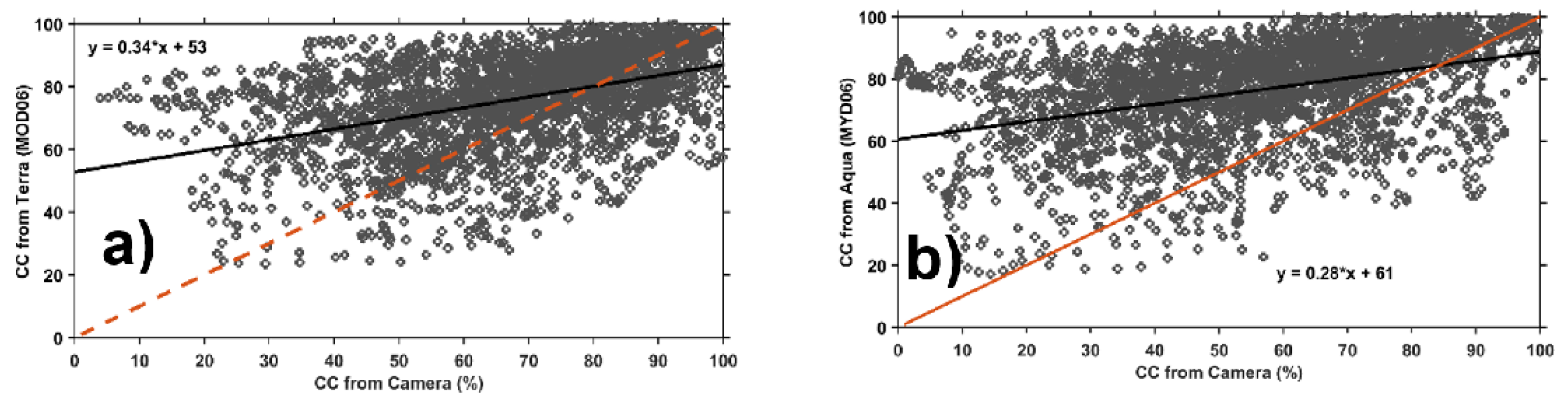
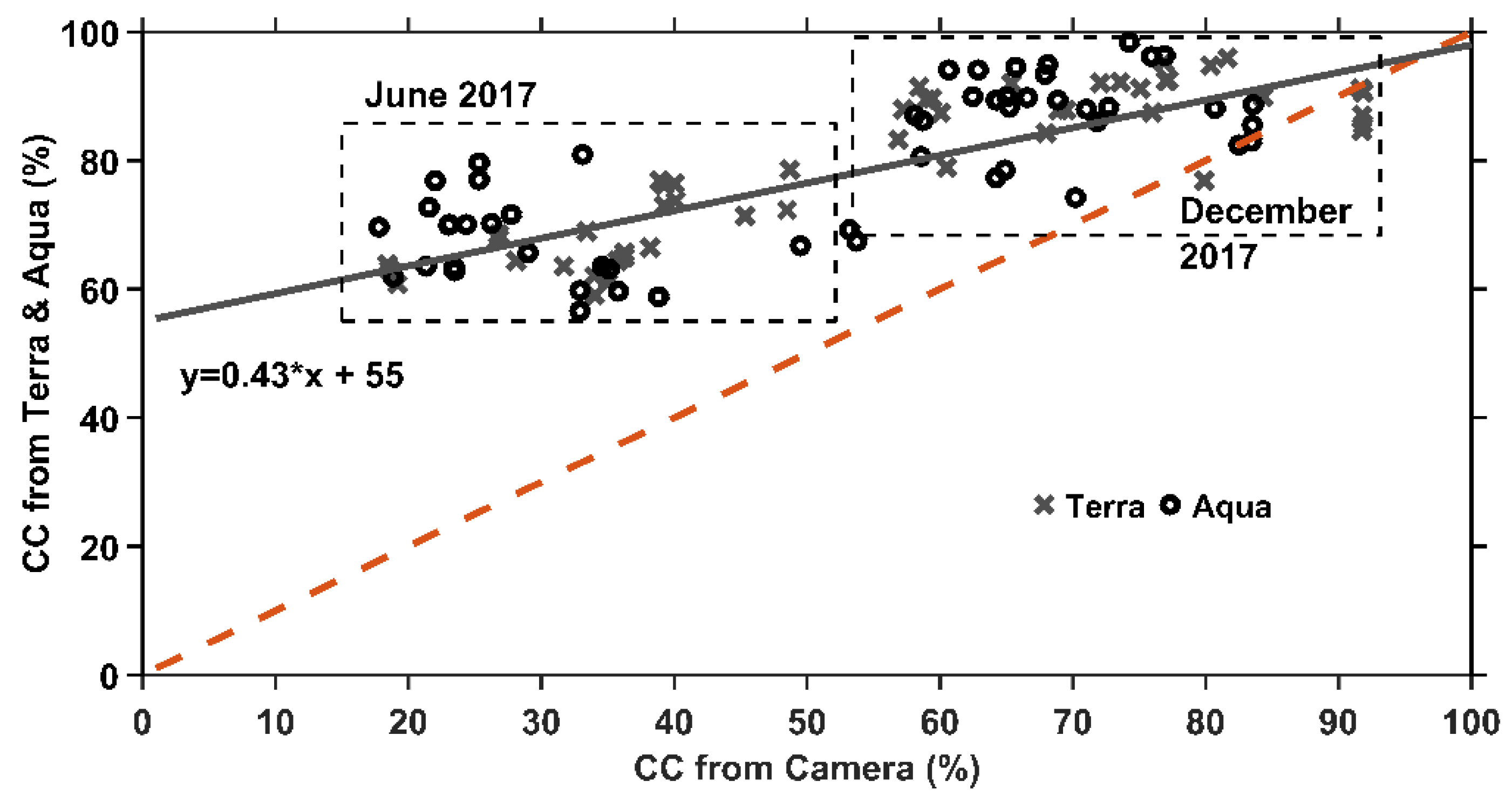
4.2. Ground Camera vs. MOD06 and MYD06 CC Products

Figure 3a,b show the relationship between the two datasets over an area of 20 km × 20 km. Two observations can be deduced when nighttime MOD06 (Terra) and MYD06 (Aqua) CCs are compared to the CC from the ground camera. First, when the camera measures low CC, Tera and Aqua’s CC values tend to be higher. Terra CC exhibits a smaller difference (24%) than Aqua CC (45%). This result can indicate low CC due to cirrus or high-level clouds CC during the 22:30 overpass of Terra. A similar result can be observed in Figure 2b,d. On the other hand, CC values from Aqua (01:30 overpass) are higher when the CC from the camera is low. Generally, CC decreases at night since ground temperature decreases and less thermal energy is released to the atmosphere [23]. Thus, the higher CC detected by Aqua for low camera CC infers the development of high-level clouds that the camera cannot effectively observe as compared with the Terra overpass time, though further studies are required to determine the spatiotemporal variation of nighttime clouds.

Cirrus reflectance cannot be retrieved from MODIS at nighttime. However, as shown in Figure 4, cirrus/high-level clouds can be confirmed from NIES lidar data. Figure 4a,b show a sample of CC from MODIS (Aqua) and the ground camera at 17:00 on 9 February 2018. In the sky image from the camera (Figure 4b), the grayscale pixels with pixel values of less than 17 can be attributed to the clear sky. The CC values from the camera and satellite are 10% and 81%, respectively. However, the time-height indicator plot of attenuated backscatter coefficient from the NIES lidar (Figure 4c) shows high-level clouds with a cloud top at around 9 km.

The mean of difference, $\overline{d},$ that results from comparing Terra (Aqua) and the ground camera datasets is −8.6 ± 35.1 (−18.9 ± 42.7). The mean absolute error, $\overline{e, }$ comparing Terra (Aqua) and the ground camera, is 24.6 (34.1). These values are lower than the values obtained when MOD08 and MYD08 data are compared with the CC from the ground camera. This implies that a smaller pixel size (5 km × 5 km) of MOD06 and MYD06 datasets can provide a better comparison with the ground camera. Nevertheless, we observe a relatively large spread in the scatter plot, which indicates high CC variability within the assigned region.

The relationship between the CCs from the detailed MODIS products (MOD06 and MYD06) and those from the camera is examined over the 200 km × 100 km area (Figure 5a,b). As expected, the results are similar to the relationships found with MOD08 and MYD08 (see Figure 2b,d). However, in Figure 5, the spread of the MOD06 and MYD06 points is evidently larger than the MOD08 and MYD08 CC products, indicating high CC variability over the same 200 km × 100 km area. Most of the points are located over the x = y line, but a number of points can be observed below the y = x line.

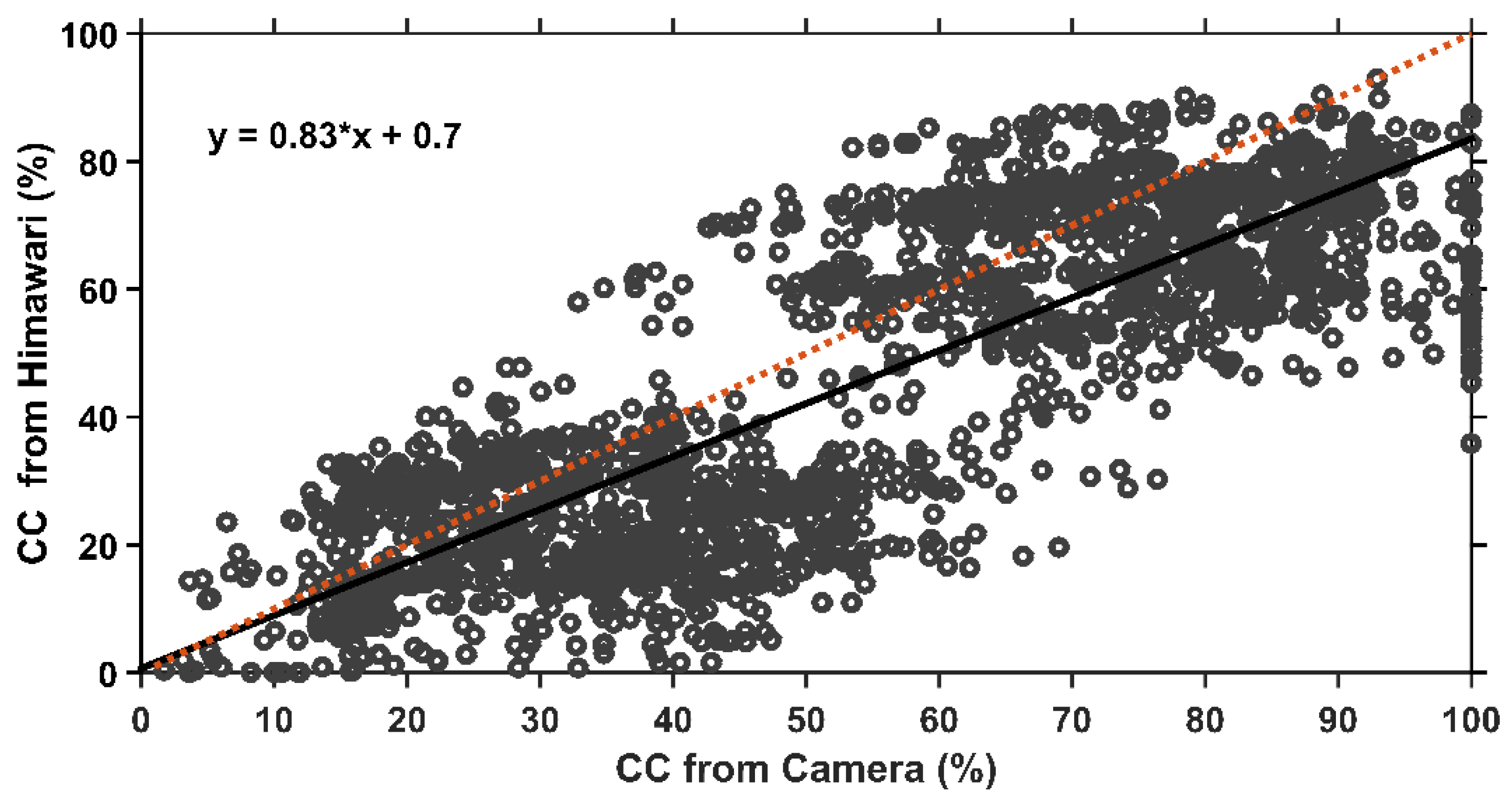
4.3. Comparison of CC from Himawari-8 and Camera

Comparing the CC from Himawari-8 with the CC from the ground-based camera shows a much better agreement, with a resulting intercept of 0.7% (Figure 6). The upper and lower groups of points in Figure 6 are the data from June and December 2017, respectively. When camera CC reaches 100%, the CC from Himawari-8 is underestimated by around 10%. The high CC from the camera usually indicates that low-level clouds are observed [23]. Thus, the lower CC of Himawari-8 means that some of the low-level clouds are not well detected by the satellite due to similar temperatures of the cloud top and the ground. The low CC from Himawari-8 when the camera observes low CC indicates that cirrus clouds are not effectively detected by the algorithm used in this study. This result can be considered a disadvantage, but since the CCs from the camera and Himawari-8 are similar to the low CC observed by the camera, this result also shows that Himawari-8 is fairly sensitive to thin clouds near the ground.

In the same two-month observation periods, CC from MOD06 (Terra) and MYD06 (Aqua) show high CC when the CC from the ground camera is low (Figure 7). The graph shows similar clusters to those seen in the Himawari-8 observations (Figure 6). The left and right clusters are the observations from December and June 2017, respectively. In December, the CC from Terra and Aqua is around three times higher than the Himawari-8 CC for a similar coverage area.

In terms of errors, comparing the CC from Himawari-8 and the ground camera yields a mean of difference, $\overline{d}$, of 8.47 and a mean absolute error, $\overline{e},$ of 10.37. These values are relatively lower than the values obtained from the comparison of CC between MODIS and the ground camera. Furthermore, the smaller pixel size (2 km × 2 km) of Himawari-8 data can better capture the temporal trends of clouds and with a more extensive spread.

When the CCs from Himawari-8 over the 200 km × 100 km area are compared with the CC from the camera, a similar result is generally observed (Figure 8), implying that the total variation of the CC between the 200 km × 100 km and 200 km × 200 km areas is not significant. With this smaller area being considered, the mean difference, $\overline{d,}$ of 12.20 and the mean absolute error, $\overline{e},$ of 30.98 are observed. The CCs from Himawari-8 are underestimated by as much as <10% when the camera observes low-level clouds. When the camera observes low CC, the CCs from Himawari-8 are less spread, indicating lower CC variation within a distance of ~100 km over the Kantō Plain area.

The high temporal characteristic of Himawari-8 is an advantage that can be used to observe the temporal variation of clouds and compare them with ground measurements. In this work, we show that the comparison of the mean CC from Himawari-8, obtained by performing a seven-point running average, shows similar patterns to ground CC for both the summer (June 2017) and winter (December 2017) months. Figure 9a and Figure 10a are the mean CC from Himawari-8 from June and December 2017, respectively, shown with the corresponding mean ground CC (Figure 9b and Figure 10b) and NIES lidar attenuated backscatter coefficient (Figure 9c and Figure 10c).

Mean CC measurements from Himawari-8 and the ground camera show similar and different patterns depending on the location of the clouds. Similar CC patterns are often observed during clear sky (2 June and 5, 18, 20, 21, and 27 December, green downward arrows in Figure 9a,b and Figure 10a,b) and 100% cloudy (3, 12, 18, 26 June, and 24 December, black downward arrows in Figure 9a,b and Figure 10a,b) conditions. The satellite and ground CC exhibit similar low CC after midnight, especially during clear conditions.

When clouds are near the ground (~2 km), Himawari-8 observations have zero or lower CC than ground CC, indicating Himawari-8’s limitation in detecting these low clouds. Such situations are observed on 8, 15, 16 June, and 4 December (red triangles in Figure 9a,b and Figure 10a,b). On 15 June, for example, a ground CC of less than 40% was observed before midnight. However, the Himawari-8-derived CC is zero. CC ≤ 40% implies the existence of broken clouds. This result suggests that Himawari-8 has some limitations in detecting these broken clouds near the ground.

When high-level (>8 km) clouds exist (6, 14,17, 20 June, and 7, 14, 15, and 28 December, represented by black triangles located at the bottom axes of Figure 9a,b and Figure 10a,b), Himawari-8 CC is higher than ground CC. When multiple cloud layers exist, as on 26 and 28 June, CC values from both satellite and ground differ from each other. CC from each sensor comes from the clouds nearest the instrument [23].

5. Conclusions

Data from the continuous monitoring of nighttime skies using a commercially available camera has provided information on the variation of nighttime CC from the ground. A comparison between the ground and MODIS (MOD08 D3 and MYD08 D3) CC datasets has shown that MODIS observes presumably high-level clouds by as much as 57% when ground CC is at 0%. This difference is larger than the previously reported comparison between the ground and AIRS CC. This result indicates that different satellites (and hence, different algorithms) have different capabilities in detecting clouds, and thus, each satellite CC product needs to be compared with ground CC separately. The comparisons of the CC from MODIS and ground camera show a higher mean of differences for MOD08 ($\overline{d}=$ 15.26) and MYD08 (23.41) compared to the MOD06 (8.55) and MYD06 (18.90) datasets. We have observed relatively smaller mean absolute errors for MOD08 ($\overline{e}=$ 16.56) and MYD08 (23.48) compared to MOD06 (24.58) and MYD06 (34.12). Providing an exact reason for these differences is still a topic that we need to explore in the future.

The comparison of CC from the camera and Himawari-8, on the other hand, shows a near 1:1 correspondence, though a scattered distribution of data points exists around the line fitting the two measurements. However, the mean of differences ($\overline{d}=$ 8.47) and the mean absolute error ($\overline{e}=$ 10.37) are smaller than those obtained from MODIS. For higher CC (~90%) measured by the camera, Himawari-8-derived CC has led to a slight underestimation (<17%). Moreover, Himawari-8 has apparent limitations in detecting low-level (~2 km) clouds with a CC ≤ 40%. Detecting these low CC is currently a challenge that we need to address in the near future by improving cloud masking algorithms. The ground-based camera has a greater CC than the CC from Himawari-8 when high-level clouds occur.

As a whole, these results indicate that knowledge of the variability of CC over a particular region can be an important piece of information when comparing satellite and ground-based CC. Both ground and satellite observations should show similar variability in CC, though some inevitable difference appears in the detection capability of low- and high-level clouds. This work further indicates the importance of the ground-based CC in providing a picture of these variations. We can explore and quantify the variations of CC with latitude and longitude from both satellite and camera by continuously operating such cameras at different locations around the globe. Correlating detected clouds from the camera and space-born lidars is one of the next steps our group will undertake in the future. Currently, our group has started a collaborative network with other researchers in Asia to achieve this goal. The data obtained from different locations can be processed using an established algorithm, ensuring and providing a uniform dataset valuable for inter-calibrating CC products from other satellites. This approach will enable bias corrections among satellite CC products, especially for low-level clouds.

References

1. Liu, Y.; Wu, W.; Jensen, M.P.; Toto, T. Relationship between cloud radiative forcing, cloud fraction and cloud albedo, and new surface-based approach for determining cloud albedo. Atmos. Chem. Phys. 2011, 11, 7155–7170. [Google Scholar] [CrossRef] [Green Version]
2. Qian, Y.; Long, C.N.; Wang, H.; Comstock, J.M.; McFarlane, S.A.; Xie, S. Evaluation of cloud fraction and its radiative effect simulated by IPCC AR4 global models against ARM surface observations. Atmos. Chem. Phys. 2012, 12, 1785–1810. [Google Scholar] [CrossRef] [Green Version]
3. Cawkwell, F.; Bamber, J. The impact of cloud cover on the net radiation budget of the Greenland ice sheet. Ann. Glaciol. 2002, 34, 141–149. [Google Scholar] [CrossRef] [Green Version]
4. Walsh, J.E.; Chapman, W.L.; Portis, D.H. Arctic Cloud Fraction and Radiative Fluxes in Atmospheric Reanalyses. J. Clim. 2009, 22, 2316–2334. [Google Scholar] [CrossRef]
5. Boucher, O.; Randall, D.; Artaxo, P.; Bretherton, C.; Feingold, G.; Forster, P.; Kerminen, V.-M.; Kondo, Y.; Liao, H.; Lohmann, U.; et al. Clouds and Aerosols. In Climate Change 2013: The Physical Science Basis. Contribution of Working Group I to the Fifth Assessment Report of the Intergovernmental Panel on Climate Change; Stocker, T.F., Qin, D., Plattner, G.-K., Tignor, M., Allen, S.K., Boschung, J., Nauels, A., Xia, Y., Bex, V., Midgley, P.M., Eds.; Cambridge University Press: Cambridge, UK; New York, NY, USA, 2013. [Google Scholar]
6. Zelinka, M.D.; Randall, D.A.; Webb, M.J.; Klein, S.A. Clearing clouds of uncertainty. Nat. Clim. Chang. 2017, 7, 674–677. [Google Scholar] [CrossRef]
7. Aebi, C.; Gröbner, J.; Kämpfer, N.; Vuilleumier, L. Cloud radiative effect, cloud fraction and cloud type at two stations in Switzerland using hemispherical sky cameras. Atmos. Meas. Tech. 2017, 10, 4587–4600. [Google Scholar] [CrossRef] [Green Version]
8. Chen, T.; Rossow, W.B.; Zhang, Y. Radiative effects of cloud-type variations. J. Clim. 2000, 13, 264–286. [Google Scholar] [CrossRef]
9. Mace, G.G.; Berry, E. Using active remote sensing to evaluate cloud-climate feedbacks: A review and look to the future. Curr. Clim. Chang. Rep. 2017, 3, 185–192. [Google Scholar] [CrossRef] [Green Version]
10. Winker, D.; Chepfer, H.; Noel, V.; Cai, X. Observational constraints on cloud feedbacks: The role of active sensors. Surv. Geophys. 2017, 38, 1483–1508. [Google Scholar] [CrossRef] [Green Version]
11. Allan, R.P. Combining satellite data and models to estimate cloud radiative effect at the surface and in the atmosphere. Meteorol. Appl. 2011, 18, 324–333. [Google Scholar] [CrossRef]
12. Norris, J.R.; Allen, R.J.; Evan, A.T.; Zelinka, M.D.; O’Dell, C.W.; Klein, S.A. Evidence for climate change in the satellite cloud record. Nature 2016, 536, 72–75. [Google Scholar] [CrossRef] [PubMed] [Green Version]
13. Bessho, K.; Date, K.; Hayashi, M.; Ikeda, A.; Imai, T.; Inoue, H.; Kumagai, Y.; Miyakawa, T.; Murata, H.; Ohno, T.; et al. An introduction to Himawari-8/9—Japan’s new-generation geostationary meteorological satellites. J. Meteorol. Soc. Jpn. 2016, 94, 151–183. [Google Scholar] [CrossRef] [Green Version]
14. Rossow, W.; Dueñas, E. The International Satellite Cloud Climatology Project (ISCCP) web site: An online resource for research. Bull. Am. Meteorol. Soc. 2004, 85, 167–172. [Google Scholar] [CrossRef]
15. Cess, R.; Udelhofen, P. Climate change during 1985-1999: Cloud interactions determined from satellite measurements. Geophys. Res. Lett. 2003, 30, 1019. [Google Scholar] [CrossRef]
16. Rossow, W.; Walker, A.; Garder, L. Comparison of ISCCP and other cloud amounts. J. Clim. 1993, 6, 2394–2418. [Google Scholar] [CrossRef] [Green Version]
17. Karlsson, K.-G.; Devasthale, A. Inter-Comparison and Evaluation of the Four Longest Satellite-Derived Cloud Climate Data Records: CLARA-A2, ESA Cloud CCI V3, ISCCP-HGM, and PATMOS-x. Remote Sens. 2018, 10, 1567. [Google Scholar] [CrossRef] [Green Version]
18. Stubenrauch, C.J.; Rossow, W.B.; Kinne, S.; Ackerman, S.; Cesana, G.; Chepfer, H.; Di Girolamo, L.; Getzewich, B.; Guignard, A.; Heidinger, A.; et al. Assessment of Global Cloud Datasets from Satellites: Project and Database Initiated by the GEWEX Radiation Panel, Bull. Am. Meteorol. Soc. 2013, 94, 1031–1049. [Google Scholar] [CrossRef]
19. An, N.; Wang, K. A comparison of MODIS-derived cloud fraction with surface observations at five SURFRAD sites. J. Appl. Meteorol. Climatol. 2015, 54, 1009–1020. [Google Scholar] [CrossRef]
20. Wang, Y.; Zhao, C. Can MODIS cloud fraction fully represent the diurnal and seasonal variations at DOE ARM SGP and Manus sites? J. Geophys. Res. Atmos. 2017, 122, 329–343. [Google Scholar] [CrossRef]
21. Ma, J.; Wu, H.; Wang, C.; Zhang, X.; Li, Z.; Wang, X. Multiyear satellite and surface observations of clouds fraction over China. J. Geophys. Res. Atmos. 2014, 119, 7655–7666. [Google Scholar] [CrossRef]
22. Werkmeister, A.; Lockhoff, M.; Schrempf, M.; Tohsing, K.; Liley, B.; Seckmeyer, G. Comparing satellite- to ground-based automated and manual cloud coverage observations—A case study. Atmos. Meas. Tech. 2015, 8, 2001–2015. [Google Scholar] [CrossRef] [Green Version]
23. Lagrosas, N.; Shiina, T.; Kuze, H. Observations of nighttime clouds over Chiba, Japan, using digital cameras and satellite images. J. Geophys. Res. Atmos. 2021, 126, e2021JD034772. [Google Scholar] [CrossRef]
24. Alonso-Montesinos, J. Real-time automatic cloud detection using a low-cost sky camera. Remote Sens. 2020, 12, 1382. [Google Scholar] [CrossRef]
25. Cazorla, A.; Olmo, F.J.; Alados-Arboledas, L. Development of a sky imager for cloud cover assessment. J. Opt. Soc. Am. A 2008, 25, 29–39. [Google Scholar] [CrossRef]
26. Gacal, G.F.; Antioquia, C.; Lagrosas, N. Ground-based detection of nighttime clouds above Manila Observatory (14.64°N, 121.07°E) using a digital camera. Appl. Opt. 2016, 55, 6040–6045. [Google Scholar] [CrossRef]
27. Klebe, D.I.; Blatherwick, R.D.; Morris, V.R. Ground-based all-sky mid-infrared and visible imagery for purposes of characterizing cloud properties. Atmos. Meas. Tech. 2014, 7, 637–645. [Google Scholar] [CrossRef] [Green Version]
28. Redman, B.J.; Shaw, J.A.; Nugent, P.W.; Clark, R.T.; Piazolla, S. Reflective all-sky thermal infrared cloud imager. Opt. Express 2018, 26, 11276–11283. [Google Scholar] [CrossRef] [Green Version]
29. Smith, S.; Toumi, R. Measuring cloud cover and brightness temperature using a ground-based thermal infrared camera. J. Appl. Meteorol. Climatol. 2008, 47, 683–693. [Google Scholar] [CrossRef]
30. Shields, J.E.; Karr, M.E.; Johnson, R.W.; Burden, A.R. Day/night whole sky imagers for 24-h cloud and sky assessment: History and overview. Appl. Opt. 2013, 52, 1605–1616. [Google Scholar] [CrossRef]
31. Souza-Echer, M.P.; Pereira, E.B.; Bins, L.S.; Andrade, M.A.R. A simple method for the assessment of the cloud cover state in high-altitude regions by a ground-based digital camera. J. Atmos. Ocean. Tech. 2006, 23, 437–447. [Google Scholar] [CrossRef]
32. Wacker, S.; Gröbner, J.; Zysset, C.; Diener, L.; Tzoumanikas, P.; Kazantzidis, A.; Vuilleumier, L.; Stöckli, R.; Nyeki, S.; Kämpfer, N. Cloud observations in Switzerland using hemispherical sky cameras. J. Geophys. Res. 2015, 120, 695–707. [Google Scholar] [CrossRef] [Green Version]
33. Wang, Y.; Liu, D.; Xie, W.; Yang, M.; Gao, Z.; Ling, X.; Huang, Y.; Li, C.; Liu, Y.; Xia, Y. Day and night clouds detection using a thermal-infrared all-sky-view camera. Remote Sens. 2021, 13, 1852. [Google Scholar] [CrossRef]
34. Long, C.N.; Sabburg, J.M.; Calbó, J.; Pagès, D. Retrieving cloud characteristics from ground-based daytime color all-sky images. J. Atmos. Ocean. Tech. 2006, 23, 633–652. [Google Scholar] [CrossRef] [Green Version]
35. Ghonima, M.S.; Urquhart, B.; Chow, C.W.; Shields, J.E.; Cazorla, A.; Kleissl, J. A method for cloud detection and opacity classification based on ground based sky imagery. Atmos. Meas. Tech. 2012, 5, 2881–2892. [Google Scholar] [CrossRef] [Green Version]
36. Heinle, A.; Macke, A.; Srivastav, A. Automatic cloud classification of whole sky images. Atmos. Meas. Tech. 2010, 3, 557–567. [Google Scholar] [CrossRef] [Green Version]
37. Li, Q.; Lu, W.; Yang, J. A Hybrid Thresholding Algorithm for Cloud Detection on Ground-Based Color Images. J. Atmos. Ocean. Tech. 2011, 28, 1286–1296. [Google Scholar] [CrossRef]
38. Yang, J.; Min, Q.; Lu, W.; Yao, W.; Ma, Y.; Du, J.; Lu, T.; Liu, G. An automated cloud detection method based on the green channel of total-sky visible images. Atmos. Meas. Tech. 2015, 8, 4671–4679. [Google Scholar] [CrossRef] [Green Version]
39. Carson, C.; Belongie, S.; Greenspan, H.; Malik, J. Blobworld: Image segmentation using expectation-maximization and its application to image querying. IEEE PAMI 2002, 24, 1026–1038. [Google Scholar] [CrossRef] [Green Version]
40. Mantelli Neto, S.L.; von Wangenheim, A.; Pereira, E.B.; Comunello, E. The use of Eucledian geometric distance on RGB color space for the classification of sky and cloud patterns. J. Atmos. Ocean. Tech. 2010, 27, 1504–1517. [Google Scholar] [CrossRef] [Green Version]
41. Gacal, G.F.; Antioquia, C.; Lagrosas, N. Trends of nighttime hourly cloud-cover values over Manila Observatory: Ground-based remote-sensing observations using a digital camera for 13 months. Int. J. Remote Sens. 2018, 39, 7628–7642. [Google Scholar] [CrossRef]
42. Ackerman, S.A.; Strabala, K.I.; Menzel, W.P.; Frey, R.A.; Moeller, C.C.; Gumley, L.E. Discriminating clear sky from clouds with MODIS. J. Geophys. Res. 1998, 103, 32141–32157. [Google Scholar] [CrossRef]
43. Frey, R.A.; Ackerman, S.A.; Liu, Y.; Strabala, K.I.; Zhang, H.; Key, J.R.; Wang, X. Cloud Detection with MODIS. Part I: Improvements in the MODIS Cloud Mask for Collection 5. J. Atmos. Ocean. Tech. 2008, 25, 1057–1072. [Google Scholar] [CrossRef]
44. Ackerman, S.; Frey, R.; Strabala, K.; Liu, Y.; Gumley, L.; Baum, B.; Menzel, P. Discriminating Clear-Sky from Cloud with MODIS Algorithm Theoretical Basis Document (MOD35). Available online: https://atmosphere-imager.gsfc.nasa.gov/sites/default/files/ModAtmo/MOD35_ATBD_Collection6_1.pdf (accessed on 12 December 2021).
45. Hubanks, P.; Platnick, S.; King, M.; Ridgway, B. MODIS atmosphere L3 gridded product Algorithm Theoretical Basis Document (ATBD) & Users Guide 2020. Available online: https://atmosphere-imager.gsfc.nasa.gov/sites/default/files/ModAtmo/documents/L3_ATBD_C6_C61_2020_08_06.pdf (accessed on 2 December 2021).
46. Yamamoto, Y.; Ishikawa, H.; Oku, Y.; Hu, Z. An algorithm for land surface temperature retrieval using three thermal infrared bands of Himawari-8. J. Meteorol. Soc. Jpn. 2018, 96B, 56–79. [Google Scholar] [CrossRef] [Green Version]
47. Minnis, P.; Kirk Ayers, J.; Palikonda, R.; Phan, D. Contrails, cirrus trends, and climate. J. Clim. 2004, 17, 1671–1685. [Google Scholar] [CrossRef] [Green Version]
Figure 1. CC difference from Terra MODIS between the top (35–37° N, 140–140° E) and bottom (35–37° N, 140–140° E) pixels.
Remotesensing 14 00960 g001
Figure 2. (a) Temporal change and (b) comparison of the mean nighttime CC from the camera and MOD08 (Terra); (c) temporal change and (d) comparison of the mean nighttime CC from the camera and MYD08 (Aqua). Two pixels of MOD08 and MYD08 (200 km × 100 km) above and including the camera location have been analyzed. The CC from Terra and Aqua shows a difference of 55% and 57%, respectively, when the camera observes low CC. The dashed line is the y = x fit.
Remotesensing 14 00960 g002aRemotesensing 14 00960 g002b
Figure 3. Comparison between CC from (a) Terra (MOD06) and (b) Aqua (MYD06) over a 20 km × 20 km area with the CC from the camera. A seven-point (~seven-day) running average is applied to both datasets to extract the relationship between the CC from MODIS and camera.
Remotesensing 14 00960 g003
Figure 4. (a) MODIS (Aqua) CC and (b) grayscale camera images on 9 February 2018 17:00 UTC (10 February 2018 02:00 JST), and (c) the corresponding lidar attenuated backscatter coefficient at 1064 nm. The small gray box in (a) indicates the location of Chiba University campus. The gray box in (c) indicates the time when the satellite and camera data were collected.
Remotesensing 14 00960 g004
Figure 5. Comparison of the camera-derived CC from (a) MOD06 (Terra) and (b) MYD06 (Aqua) over a 200 km × 100 km area. A seven-point (~ seven-day) running average has been applied to both datasets to extract the relationship between the CC from MODIS and camera. The dashed line is the y = x fit.
Remotesensing 14 00960 g005
Figure 6. Comparison of the mean CC from Himawari-8 over a 200 km × 200 km area (10,000 pixels) and the ground camera for the month of June and December 2017. The mean CC from Himawari-8 is obtained by applying a seven-point average of all data at a particular time. The dashed line is the y = x fit.
Remotesensing 14 00960 g006
Figure 7. Average CC from Terra and Aqua (5 km pixel resolution in the 20 km × 20 km area) and from the ground camera observed in June and December 2017.
Remotesensing 14 00960 g007
Figure 8. Comparison of the mean CC from Himawari-8 over a 200 km × 100 km area (5000 pixels) and the ground camera for the months of June and December 2017. The mean CC from Himawari-8 are obtained by applying a seven-point average of all data at a particular time. The dashed line is the y = x fit.
Remotesensing 14 00960 g008
Figure 9. Temporal plots of the CC data observed in June 2017 from (a) Himawari-8, (b) ground camera, and (c) the corresponding attenuated backscatter from the NIES lidar. Green and black downward arrows indicate the day with the clear sky and totally cloudy sky, respectively. Red and black triangles indicate the day when low- and high-level clouds are observed.
Remotesensing 14 00960 g009
Figure 10. Temporal plots of the CC data observed in December 2017 from (a) Himawari-8, (b) ground camera, and the corresponding (c) attenuated backscatter from the NIES lidar. Green and black downward arrows indicate the day with the clear sky and totally cloudy sky, respectively. Red and black triangles indicate the day when low- and high-level clouds are observed.
Remotesensing 14 00960 g010
Publisher’s Note: MDPI stays neutral with regard to jurisdictional claims in published maps and institutional affiliations.