Article

SmartWater: A Service-Oriented and Sensor Cloud-Based Framework for Smart Monitoring of Water Environments

1
College of Computer Science and Engineering, Taibah University, Medina 42353, Saudi Arabia
2
SMART Laboratory, Jendouba University, Jendouba 8189, Tunisia
3
Security Engineering Laboratory, CCIS, Prince Sultan University, Riyadh 12435, Saudi Arabia
4
RIADI Laboratory, University of Manouba, Manouba 2010, Tunisia
5
Robotics and Internet-of-Things Laboratory, Prince Sultan University, Riyadh 12435, Saudi Arabia
*
Author to whom correspondence should be addressed.
Remote Sens. 2022, 14(4), 922; https://doi.org/10.3390/rs14040922
Submission received: 22 December 2021 / Revised: 29 January 2022 / Accepted: 1 February 2022 / Published: 14 February 2022
(This article belongs to the Special Issue Big Data Analytics for Secure and Smart Environmental Services)

Abstract

:
Due to the sharp increase in global industrial production, as well as the over-exploitation of land and sea resources, the quality of drinking water has deteriorated considerably. Furthermore, nowadays, many water supply systems serving growing human populations suffer from shortages since many rivers, lakes, and aquifers are drying up because of global climate change. To cope with these serious threats, smart water management systems are in great demand to ensure vigorous control of the quality and quantity of drinking water. Indeed, water monitoring is essential today since it allows to ensure the real-time control of water quality indicators and the appropriate management of resources in cities to provide an adequate water supply to citizens. In this context, a novel IoT-based framework is proposed to support smart water monitoring and management. The proposed framework, named SmartWater, combines cutting-edge technologies in the field of sensor clouds, deep learning, knowledge reasoning, and data processing and analytics. First, knowledge graphs are exploited to model the water network in a semantic and multi-relational manner. Then, incremental network embedding is performed to learn rich representations of water entities, in particular the affected water zones. Finally, a decision mechanism is defined to generate a water management plan depending on the water zones’ current states. A real-world dataset has been used in this study to experimentally validate the major features of the proposed smart water monitoring framework.

1. Introduction

Water is essential and vital for sustaining human life on earth. Although about 71% of the earth is covered with water, only 3% of the world’s water is freshwater, and two-thirds of this water is hidden in glaciers that are frozen or not available for use [1]. Besides, most of the world’s people lack clean and safe drinking water. Drinking water is defined, according to World Health Organization (WHO) and the United States Environmental Protection Agency (USEPA) guidelines [2,3], as water that presents no risks to human health over a lifetime of consumption, including different sensitivities that may arise between stages of his life. Every year, millions of people around the world suffer from various fatal diseases caused by drinking water pollution. The WHO stated in its report, which is released in June 2019 (https://www.who.int/news-room/fact-sheets/detail/drinking-water, accessed on 15 November 2021) that “Globally, at least 2 billion people use a drinking water source contaminated with feces. Contaminated water can transmit diseases, such as diarrhea, cholera, dysentery, typhoid, and polio. Contaminated drinking water is estimated to cause 485,000 diarrhea deaths each year”. The WHO also states that, by 2025, half of the world’s population will be living in water-stressed areas. These facts show the severe threats and diseases caused to the global population by water scarcity, which encompasses water availability and quality.
Today, with the exponential increase in water use due to the rapid development of the human population, ensuring a safe and accessible water supply is a vital need for all. An effective smart water management system is a must in order to avoid the severe repercussions of water scarcity. In recent years, significant efforts have been made to monitor water quality using a set of Key Performance Indicators (KPIs), such as temperature, the potential of Hydrogen potential (pH), dissolved oxygen, turbidity, conductivity, etc. [4,5,6,7]. The measures of these KPIs are collected and analyzed using IoT platforms. To rationalize water consumption, with the goal of achieving a reduction in consumption, several water management systems have been developed using different technologies. However, the main drawback of these attempts is the high cost and energy consumption [8,9].
Over the past few years, the Internet of Things (IoT) technology has gained significant prominence in several areas, and this is thanks to its added-value capabilities and competitive advantages [10,11,12]. IoT enables the control and processing of information in its ecosystem in order to provide smart applications in different domains, including the water management domain. In this context, the IoT consists of networks of smart devices equipped with physical sensors that collect and monitor water data. For analysis, the latter are transferred to computational platforms. IoT-based water management systems are low-cost solutions that can be easily scaled up while guaranteeing easy access for remote monitoring and control. In fact, low-cost sensors are efficient for measuring water quality indicators. In addition, the adoption of commonly used communication technologies by the IoT allows the deployment in pre-existing systems with few configurations and adaptations carried out.
In the present work, the main objective is to develop a smart water solution to support different water stakeholders (e.g., water and sanitation institutions, agricultural and environmental sectors, farmers, urban consumers, industrial consumers, etc.) in controlling and protecting their provisioned/consumed water resources. To achieve this goal, a novel IoT-based framework is defined to ensure the smart monitoring of water environments. The main contributions are summarized as below:
  • Designing a service-oriented and an IoT-based multi-layer framework that transforms the water environments into smart zones endowed with sensing and intelligent management capabilities.
  • Modeling the water environment as a knowledge graph [13] that defines the involved elements, including water entities, sensors, water problems, monitored data, water management operations, etc. Such a multi-relational and semantic structure will serve as a dictionary that encompasses each information related to the water environment.
  • Exploiting network embedding [14,15] to learn semantics and enrich representations of water entities incrementally and to map them into a low-dimensional vector space according to their similar features, behaviors, and deviations. This step helps classify the affected water entities and efficiently select and trigger the appropriate corrective measures.
  • Defining a decision mechanism that recommends the appropriate management plan for each class of water problem. This mechanism reduces the complexity of exploring the whole network of water entities and their management costs.
  • Evaluating and validating the developed solution through several use-cases representing relevant water problems (e.g., sediment detection, bacterial contamination, discoloration, etc.) and using a real-world dataset.
The rest of this paper is organized as follows. Section 2 discusses recent state-of-the-art solutions related to IoT-based water management. Section 3 details the architecture of the proposed framework for water quality monitoring. Section 4 and Section 5 introduce the water knowledge graph (WKG) and the way it is updated at each monitoring time frame. In Section 6, an incremental embedding method is proposed to map the water network into a low-dimensional vector space and to classify its content for the decision purpose. In Section 7, a decision mechanism is defined based on the classification of affected water entities. Implementation and experimental analysis are provided in Section 8. The summary of this work and the future research directions are provided in Section 10.

2. Related Work

Many causes have engendered water scarcity in several regions of the globe, such as climate change, altered meteorological conditions, including droughts or floods, increasing pollution, growing human demand, excessive water usage, global warming, governmental access, local conflicts, illegal dumping, and natural catastrophes. To face the dramatic consequences of water scarcity, real-time water management is a critical necessity to ensure a sustainable and safe water supply. Recently, the application of new technologies such as IoT [16,17] and service and cloud computing [18,19,20,21] have proved their efficiency in the water sustainability field [22]. In the present study, the focus is on reviewing the use of these technologies in the context of water scarcity management.
Using IoT and remote sensing technologies, the authors in [23] presented a smart water quality monitoring system. For analysis, the proposed system measures four water parameters KPIs (pH, Oxidation-reduction potential (ORP), conductivity, and water temperature) using remote sensors. The collected data are transferred to a cloud server, where the data analysis is performed. For the validation of the system’s measurement accuracy, four different water sources were tested within a period of 12 h at hourly intervals.
Shahanas et al. [24] developed a Smart Management Water (SMW) system based on IoT techniques and analytics. The authors collected their dataset manually. The proposed solution starts by collecting the water level from different tanks using smart sensors. These collected data are transferred to a centralized server using Arduino and Raspberry Pi to be analyzed, then visualized through a Web interface. The proposed solution allows the detection of the water level in a tank. When the level goes below a threshold, an alert will be sent to the users.
In [25], the authors presented a context-aware ontology-driven approach to ensure the right water resource management in a smart city. The developed approach is based on the Multimedia Web Ontology Language (MOWL) and consists of three layers: data acquisition layer, context-aware service layer, and application layer. The first layer is responsible for collecting data from different sources through heterogeneous IoT devices such as climate and water-level sensors. Since the collected data are in various formats, they are converted into a predefined RDF format in the second layer resulting in MOWL files. These ontologies support the Dynamic Bayesian Network (BBN), which is responsible for analyzing data and predicting the changing situations in real time. The last layer ensures a clear presentation of the learned knowledge to the water authorities and determines the appropriate recommendation or warning to take suitable actions.
Myint et al. [26] designed a Water Quality Monitoring (WQM) system for IoT environments based on a reconfigurable smart sensor network. The proposed WQM system collects five water-related data measurements, including pH, water level, turbidity, carbon dioxide on the water’s surface, and water temperature. These data are accumulated from multiple sensor nodes in parallel, in real-time, and at high speed, to be finally checked for monitoring. WQM minimizes the time and cost of detecting water quality, contributing to smart environmental management.
Simmhan et al. [27] proposed a smart water management application for smart city utilities. The system architecture is based on open Web standards and involves network protocols, cloud computing, edge resources, and big data platforms. The proposed software has been tested on a smart campus at the Indian Institute of Science (IISc). The results have shown the scalability of the application to be applied in the city or for other areas of intelligent utilities.
Mukta et al. [28] proposed an IoT-based system for Smart Water Quality Monitoring (SWQM) based on four parameters collected using IoT sensors. The used metrics include water temperature, pH, electric conductivity, and turbidity. SWQM system analyzes the extracted sensor data using a fast forest binary classifier to determine whether the tested samples of water are drinkable or not. The performance of this classifier is compared with three other binary classifiers, including support vector machine, logistic regression, and average perceptron algorithms. Among these techniques, the fast forest binary classifier provided the highest accuracy for the same test data. In their work, Mukta et al. used this classifier to develop a desktop application named “Sprinkle: Water Quality Checker” that monitors and assesses the water quality.
Liu et al. [29] proposed a method based on Long Short-Term Memory (LSTM) deep neural networks to predict the quality of the drinking water in IoT-based environments. For model training, the authors used the water quality monitoring data collected by the automatic monitoring station of Guangzhou Water Source in Yangzhou City for the two years 2016 and 2017. The collected data include temperature, pH, dissolved oxygen, conductivity, turbidity, chemical oxygen demand, and ammoniacal nitrogen (NH3–N). To assess the effectiveness of the proposed model, the predicted results were compared to the measured data. The experimental results have shown that the proposed model offers a feasible approach for predicting the quality of drinking water.
In [30], a real-time water quality measurement system called Smart Water Quality Monitoring System (SWQMS) was proposed. SWQMS is capable of investigating and providing information related to the local water quality by monitoring four key performance indicators, which are temperature, pH, oxidation-reduction potential, and conductivity. This system is designed on the basis of IoT technologies integrated within a network of wireless sensors. SWQMS is tested to monitor various water sources available in Fiji like coasts, coves, seas, rivers, and taps. The obtained data are analyzed using statistical methods and verified by comparing them to the Fiji national drinking water quality standards.
In [31], a semantic modeling method based on ontologies and rules building was proposed to monitor the water quality of rivers and to process relevant observational data. It is based on the Observation Process Ontology (OPO) and allows the description of semantic properties related to water resources and the collected observation data. In addition, it can provide semantic relevance among the different concepts involved in the water quality monitoring process. OPO is constructed on the basis of the DOLCE Ultra-Light ontology.
A water management information system architecture, based on the micro-services paradigm and called WISdoM, was proposed in [32]. WISdoM integrates core functionalities that support the implementation of three use cases of water utilities, namely: long-term water demand forecasts, groundwater data management, and precipitation data management. WISdoM uses several internal and external data sources (e.g., precipitation data, water consumption data, weather data, etc.). Each data source is encapsulated by a micro-service that allows querying the desired data. Data sources can be combined using a message broker service that ensures data reception from different sources. The applicability of the proposed approach and the usability of WISdoM are evaluated by expert users and by executing different scenarios.
The goal of the work presented in [33] is the implementation of near-term and iterative ecological predictions for freshwater management. A forecasting framework named FLARE was developed to help manage water quality in critical lakes and reservoir ecosystems. Flare uses water quality sensor observations and models to make forecasts of future water quality conditions (i.e., temperature and dissolved oxygen). Forecasts provided by Flare are used by decision support tools for managers. Remote management and transfer orchestration of observations data and decisions are ensured by cloud computing tools.
An architecture for water quality monitoring for an irrigation precision agriculture system was provided in [34]. The canals for irrigation, the fields, and the urban areas were all considered. The data were being sent via both WiFi and LoRa wireless technologies, with the cluster head node, serving as a WiFi/LoRa bridge that connects the WiFi and LoRa nodes. A tree topology for LoRa with several hops was also provided. This tree enabled for greater distances to be covered while also lowering the quantity of data and messages transferred from one node to another. A heterogeneous communication protocol for a precision agricultural system was also proposed. The protocol was intended to allow communication between devices that use WiFi and LoRa communication technologies. To assess the performance of the proposed protocol, tests were carried out in a real-world context using WiFi and LoRa nodes.
It is clear from the above attempts that water monitoring is essential to ensure the appropriate resource management and provide adequate water supply to the citizens. Efficient management of water requires the identification of the prevailing causes of water scarcity in a geospatial environment. This identification is ensured by analyzing the historical and real-time water-specific information captured through IoT sensor networks. To deal with uncertainties in water resources, a context-aware approach is also needed to predict environmental and climate change and offer timely guidance to the local water authorities. This approach will provide accurate knowledge of the available water resources to meet the competing demands. Besides, a knowledge management system ensuring water flow and quality modeling is needed to predict the drinking-water quality in the future and offer tracking capabilities to manage the issues generated as consequences of water shortages.
Analyzing the above water monitoring systems, the following major drawbacks have been identified:
  • Most approaches concentrate on the monitoring phase without providing an understanding or taxonomy of water environment entities. Although some attempts have used ontologies to represent the semantics of water-related information, the specification of the water environment entities (water objects, water sensors, management policies, etc.) is performed in isolation, which may lead to conflicting or failed corrective measures. A possible solution to this issue is to provide a semantic and multi-relational modeling of the water network through the use of knowledge graphs [13] that allow us to explicitly represent the relationships between entities of the smart water environment.
  • Existing water monitoring systems suffer from scalability and management complexity issues due to the large size of the water networks and the huge volume of water data. This fact leads to an inaccurate analysis of the collected water information and may affect the decision on the water management operations (e.g., predictions, warnings, recommendations). Aiming to face the high computational cost caused by the analysis of the water resources’ monitored data, the incremental representation learning of the water network could be an elegant solution. To this end, metapath2vec [35] is applied as an embedding technique ensuring the application of incremental learning of partial changes in the water information network (WIN).
  • Current monitoring systems trigger water management actions for each detected event (e.g., change in the water level), which leads to an increase in the cost of treating abnormal/failed aquatic objects. Since some water areas may experience the same deviations or degradation in water quality, the idea is to exploit the representations learned from the water zones’ features to classify them according to their common features/problems. This enables the appropriate water management plan to be triggered for each class of water zones rather than treating each zone in isolation.

3. Sensor Cloud Architecture for Smart Water Monitoring

The proposed monitoring framework, called SmartWater, is abstracted and summarized in the form of a layered service-oriented system that runs based on a distributed sensor-cloud architecture (see Figure 1).
The proposed framework is composed of four layers: smart sensors’ layer, data management layer, workflows layer, and water analytics layer.
  • Smart sensors layer: This layer is based on a sensor-cloud architecture that transforms the water environment into a set of smart and self-monitored water zones. This layer utilizes well-known computing paradigms, such as autonomic computing, sensor networks, and reinforcement learning. The synergy between these technologies will endow the sensors at each water zone with autonomic and analytics capabilities that will offer an intelligent control of water zones’ states.
  • Data management layer: This layer represents the data processing and management facilities that allow realizing various operations on the water data, which were previously collected and outputted by a cloud of sensors. To achieve this goal, this layer takes advantage of service-oriented computing (SOC) paradigm to define a set of sensor-cloud services that perform various data management operations. These operations are achieved thanks to the combination of robust analysis and reasoning methods and tools, including machine learning, auto-scaling, ETL (Extract-Transform-Load) [36], filtering and aggregation, data storage, micro-services, etc.
  • Water workflows layer: This layer serves as a repository of abstract water management plans. Depending on the water zones’ current status, i.e., captured events, a plan is triggered by invoking the corresponding water management workflow. Using software reuse principles, this latter is instanciated by orchestrating the appropriate sensor cloud services from the data management layer, to be aggregated as executable workflows that perform advanced water management operations.
  • Water analytics layer: At the higher level of the smart water’s surveillance system, a set of predefined workflow templates denotes the decision support and recommendations regarding the state of water zones. Taking advantage of techniques, such as collaborative filtering, predictive analytics, knowledge-based reasoning, as well as other emerging technologies from Google (e.g., knowledge graphs), a recommendation module will be defined to allow triggering the appropriate water management actions.
The water zones’ monitoring and management process is summarized in Figure 2.
After transforming the water zones’ information into a knowledge graph structure, the monitoring phase starts at each water zone. The data collected by water quality sensors are, then, filtered and employed to update the WKG. This change in the WKG triggers the re-embedding of the water network’s entities by incrementally learning the new representations of the ones affected by changes. At this stage, the new distribution of water entities in the embedding space is used to group these latter according to their similar states (e.g., poor water quality). Finally, each class of problem (e.g., leakage) is mapped to a corrective measure, by evaluating the available water management policies. The whole routine is repeated following a monitor-learn-decide loop. As depicted in Figure 2, the smart sensors layer is in charge of the water zones’ monitoring activity. The data management layer is responsible for: (i) modeling the smart water environment, (ii) updating the water information network, and (iii) selecting the corrective actions. As for the water workflows layer, it will assist the data management layer in determining corrective actions. Finally, the water analytics layer will be involved in the re-embedding of the water information network, as well as the classification of water zones to ensure their management.

4. Modeling of Smart Water Environment

The first step towards intelligent monitoring of water zones is the correct representation of its related information. Given the complexity, heterogeneity, and large-scale nature of the water network, which requires multi-relational and semantic modeling of its elements, the present approach exploits the strengths of knowledge graphs [37] as a recent Google technology to explicitly represent the relationships among smart water environment’s entities (see Figure 3). This new kind of knowledge base was launched, for the first time, in 2012 by Google. Since then, it has been adopted by leading service companies, such as Amazon, Facebook, IBM, Yahoo, etc. These latter’s services (e.g., search, recommendation, advertising, etc.) have been improved thanks to knowledge graphs’ abilities to represent and store complex relationships between real-world entities [37].
In the present approach, the WKG, also called Water Information Network includes various entities, such as sensors, services, water stations and data, water workflows, management plans, etc. Such entities are the cornerstone of each water zone.
Definition 1.
(Water Knowledge Graph) is an heterogeneous information network G = ( V , E , F , D + ) , where nodes in V = < V s , V c , V f , V z > denote the set of water-related entities (sensors, services, water zones, management policies, etc.), edges in E correspond to the connections between the water environment’s actors, and F is the set of features characterizing the water network’s entities. D + = { ( e i , r , e j ) } denotes the set of facts (triples) in G . A fact is a 3-tuple f = ( v i , r , v j ) , where v i , v j V are the head and tail entities (e.g., sensors, monitoring hubs, distribution pipelines, management rules, etc.), and r E denotes a relation (connection) between v i and v j . A relation r : v i r v j E in the WKG is a typed link (e.g., Monitor, ManagedBy, Trigger) between entities v i and v j .
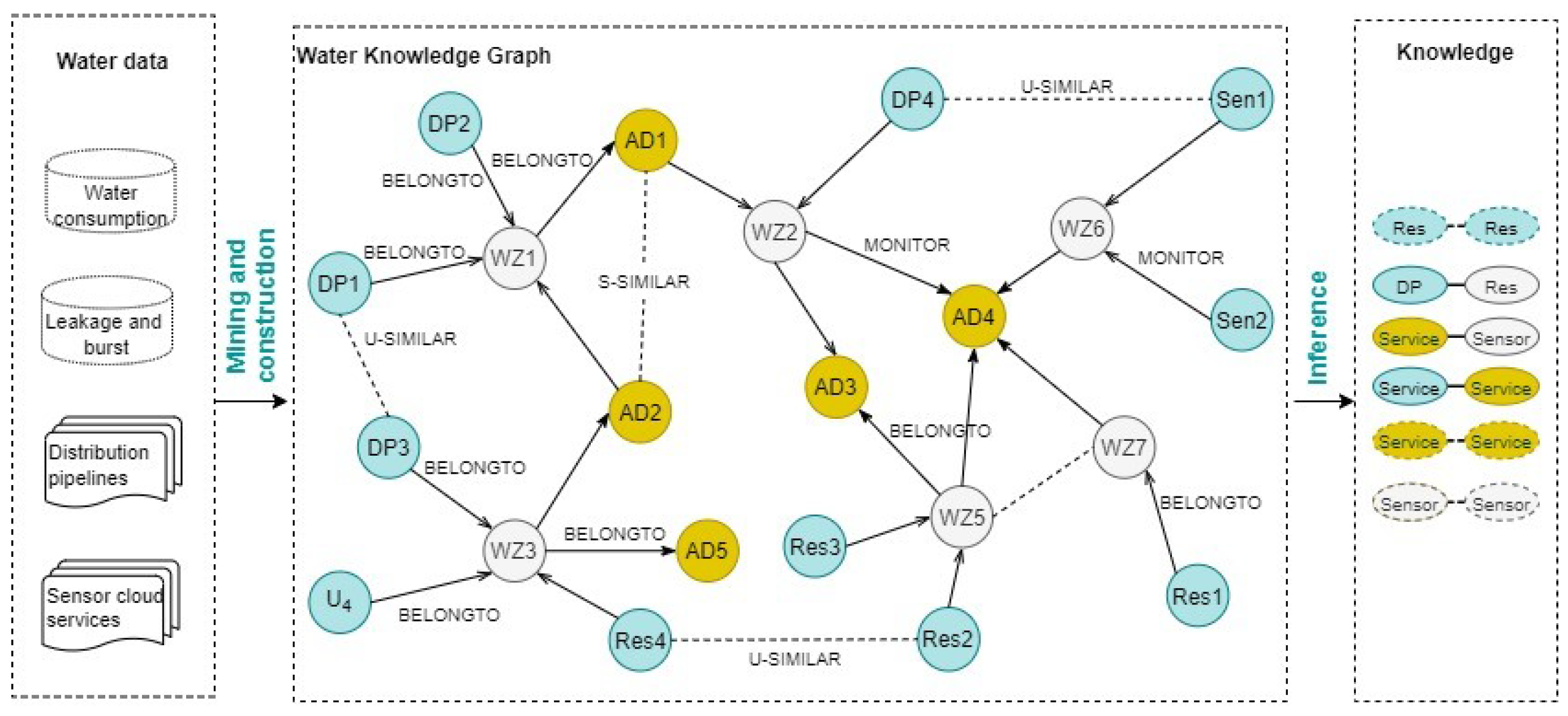
Figure 3 shows the software and hardware entities that are involved in the construction of the WIN. Examples of hardware entities include storage reservoirs (Res), distribution pipelines (DP), IoT water sensors (Sen), water supply chain components (SCC), pump stations (PS), water transportation pipelines (TP), rain gauges (RG), smart meters and monitoring hubs (MH) for measuring consumption, acoustic devices (AD) for real-time leakage detection, pressure monitoring hubs (PMH) for leakage detection and pump optimization, etc. Other types of entities include services (e.g., sensor cloud services) and water’s smart management policies (e.g., leakage prediction, burst repair, etc.), which are related to the different water zones (WZ).
Since the WKG results from the aggregation of various types of resources, it is treated as a combination of information sub-networks, also called views [38]. In fact, the WKG can be seen as a multi-view information network, where each view denotes a sub-network of knowledge (see Definition 2). For instance, the sensors’ view ( ϕ s e n ) denotes all of the information regarding the hardware entities that are responsible for monitoring the water zones. Whereas the services view ( ϕ s e r ) is a sub-network of G that groups all the information regarding the value-added and sensor cloud services that process, transform, and aggregate water zones’ data. Each water zone could also be modeled as a view of the water network.
Definition 2.
(Water view) A view ϕ i = ( V i , E i , F i , D i + ) is a sub-network of the water network G = ( V , E , F , D + ) , where V i V is a subset of nodes, F i is a subset of features specific to the elements of the i t h water zone Z i , and E i E is the subset of relations r E i within Z i . The whole WKG can be seen as the aggregation ϕ of all views, where ϕ = { ϕ 1 ϕ 2 ϕ k } .

5. Water Zone Monitoring

This section is devoted to the description of SmartWater’s sensing capabilities, as well as some examples of water monitored data. It also shows how the monitored data are processed to decide on the water zones’ states and update the WKG.

5.1. Sensing Capabilities

Sensors can detect events or changes in their surroundings and send the data to other connected electronic devices. Chemical, physical, and biological aspects of water can all be detected with sensors. In this work, to identify the water regions that suffer from qualitative problems, the smart water management system takes advantage of numerous sensors that form a cloud of IoT objects. The distribution of sensors depends on each zone’s requirements and restrictions. These requirements include the monitoring range, the response time, the data interference, and the sensitivity measurements, etc. Despite the enormous number of water monitoring KPIs [39], only a limited number of significant parameters is used to monitor water quality [40,41].
The proposed Smart water solution can be used in many applications, such as water and sanitation institutions, agricultural and environmental sectors, farmers, urban consumers, and industrial consumers. Each of these applications requires a specific type of sensors to be involved in the IoT solution. Table 1 depicts some examples of water sensors that can be used. The type of sensors included in the IoT solution depends on the type of application of the Smart water system. The proposed solution aims to reduce the time required for gathering data and includes advanced analytics that can measure, catalog, and analyze the acquired data.
The integration of sensors with cloud computing, as depicted in Figure 1, transforms the bottom layers as a cloud of sensors [45]. The motivation behind using Sensor-Cloud [46] lies in the numerous advantages that this promising technology offers in terms of large-scale data sharing and mining, cloud-based powerful and low-cost computational and storage resources, and automatic provisioning and supervision provided by virtualized sensor services. This highly scalable infrastructure not only enables the smart water management system to gather, filter, and aggregate water-related data, but also access, process, and store a huge volume of collected data, thanks to the computing capabilities offered by the cloud resources. These latter include a kind of sensor cloud services endowed with analytics and learning capacities, such as MLaaS (Machine Learning as a Service) and DLaaS (Deep Learning as a Service) to help infer valuable knowledge and recommend adequate water management plans. As presented by the novel SmartWater framework, the data collected by the various water quality sensors is transmitted to the cloud storage. Then, they are filtered and verified by cloud services and compared with previously specified threshold values. Each cloud service can manage one or more sensors depending on the size of the water zone and the amount of data collected. The data collected are mined by various services (e.g., MLaaS and DLaaS) so that abnormal states of water zones are identified and addressed in real-time, ensuring, therefore, the selection of the appropriate corrective action that will be applied.

5.2. Water Management Policies

The selection of the appropriate water management operations mainly depends on the water quality and the water zones’ hardware capacities. In fact, in each zone, water sensors and monitoring hubs collect useful data, such as pH, water temperature, turbidity, conductivity, dissolved and chemical oxygen demand, NH3–N, hardness, solids, amount of chloramines, amount of sulfates, electrical conductivity, organic carbon, trihalomethanes, potability, etc. Using these real-time data, the distributed autonomic service-based managers decide about the appropriate water management policy and corrective measures, taking into account the filtered, aggregated, and analyzed water data. The water measurements are evaluated against the WHO’s standard values (https://www.who.int/publications/i/item/9789241549950, accessed on 15 November 2021). Then, they are transformed into usage patterns (e.g., leakage, burst, over-consumption, quality of raw catchment water, changes in the storage reservoirs’ levels, pressure in the distribution pipeline, etc.) that will be exploited to run over the WKG and locate the appropriate management operations. Other events can be detected using sensors or direct video surveillance. Examples include contaminated hydrants, defective pipes and leaks, contamination during repair and maintenance of tanks and pipes, toxic substances in pipe materials, cross-connections between potable water storage tank and non-potable water storage tank or pipe, damage to wire mesh in overflow or vent pipe, defective back-flow preventers at outlets throughout the distribution system. Table 2 depicts some examples of corrective actions and their triggering events, following the ECA (Event-Condition-Action) rules representation.
The monitoring and prediction of each water zone’s state are performed at each time frame t. The granularity of the time periods (minutes, hours, days, etc.) depends on the frequency of changes in water quality and the requirements of each water zone. In this version, for simplicity reasons, the time variable t is considered as a traditional window time. The variable t means the number of observations (i.e., sample data) in t periods. In this work, the monitoring history is modeled as a set of matrices, where each one corresponds to the data collected from a specific water zone (see Table 3). As shown by Table 3, rows represent the water features, whereas columns denote the monitoring timeframes. Entries correspond to the collected data by water IoT sensors. For instance, the collected data at time t is represented by the column ( P H = 8.5 , T D O = 3.1 , T e m p e r a t u r e = 37 , T u r b i d i t y = 0.42 ).
The management operations are triggered when the analysis of water changes after each time period t results in at least one affected water zone. Once the monitoring task is performed, the water state at time t + 1 is outputted, and the water quality or eventual problems are deduced. The WIN is then updated by considering the new features of each water zone. The updated WIN in Figure 4 shows that the abnormal behaviors are represented by labeled nodes (see red colors) denoting the deviation patterns. That will facilitate and accelerate the selection of corrective plans/actions by adopting a classification of the WIN nodes with similar features/states, as will be demonstrated in the next section.

6. Smart Water Analytics Based on Network Representation Learning

Once the WKG is updated based on the monitoring data, the next step is to select and trigger the corrective measures for each infected water zone. However, the water environment’s large-scale and complex nature makes it challenging to explore the WKG to locate suitable management operations. Since several water zones may encounter similar problems, classifying their elements (pipelines, reservoirs, etc.) according to their current states (e.g., pipelines’ pressure level) will accelerate the decision process.
To achieve this goal and to reduce the complexity of processing such a huge information network, network representation learning (NRL) [14] is adopted, as an efficient solution to project the WKG into a low-dimensional vector embedding space, in which the nodes with similar features will be close and classified together. For example, the distribution pipelines with abnormal behavior will be tight in the vector space, whereas the storage reservoirs with similar capacities and the reservoirs with non-drinkable water will be mapped into the same vector embedding space. This powerful approach will allow performing various tasks (e.g., classification, clustering, link prediction, anomaly detection, etc.) on the information network’s content in an efficient and accurate manner [14]. In the present work, learning the representation of water network nodes is the first step towards efficiently performing some of the following downstream tasks: clustering of sensed data, classification of drinking and non-drinking water zones, repair or substitution of failed hubs or services, anomaly detection at each water zone, etc.
In this paper, a water-specialized network embedding method is proposed to infer meaningful representations of water zones. The proposed method maps the water objects into a low-dimensional vector space. To learn the semantics of water-related information, metapath2vec is adopted, as an incremental embedding technique [
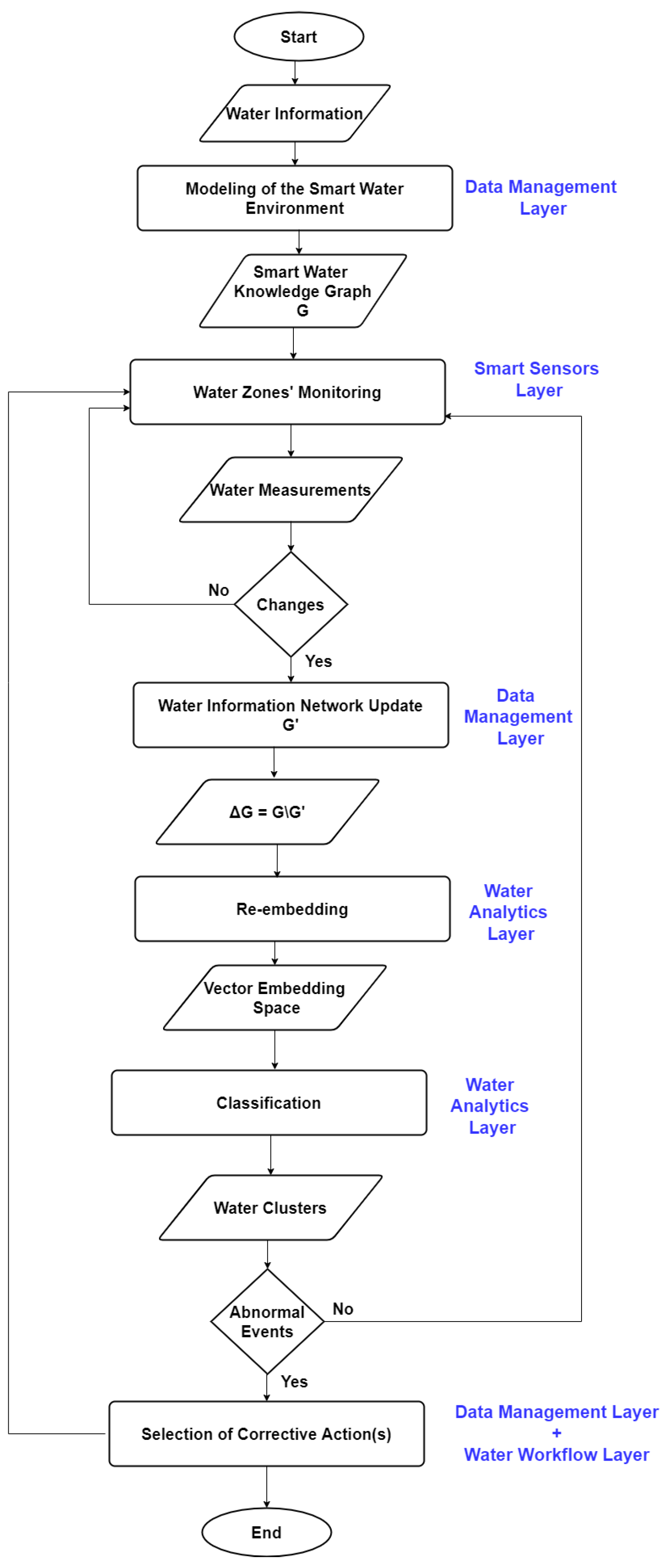
35]. Suitable for dynamic and heterogeneous information networks, the proposed method first learns the embeddings of each node in the water network. Then, at each monitoring time-frame, incremental learning is applied to the updated water network to take the new changes (e.g., water zones’ state) into consideration and to update the closeness degrees between water entities (see Figure 2).
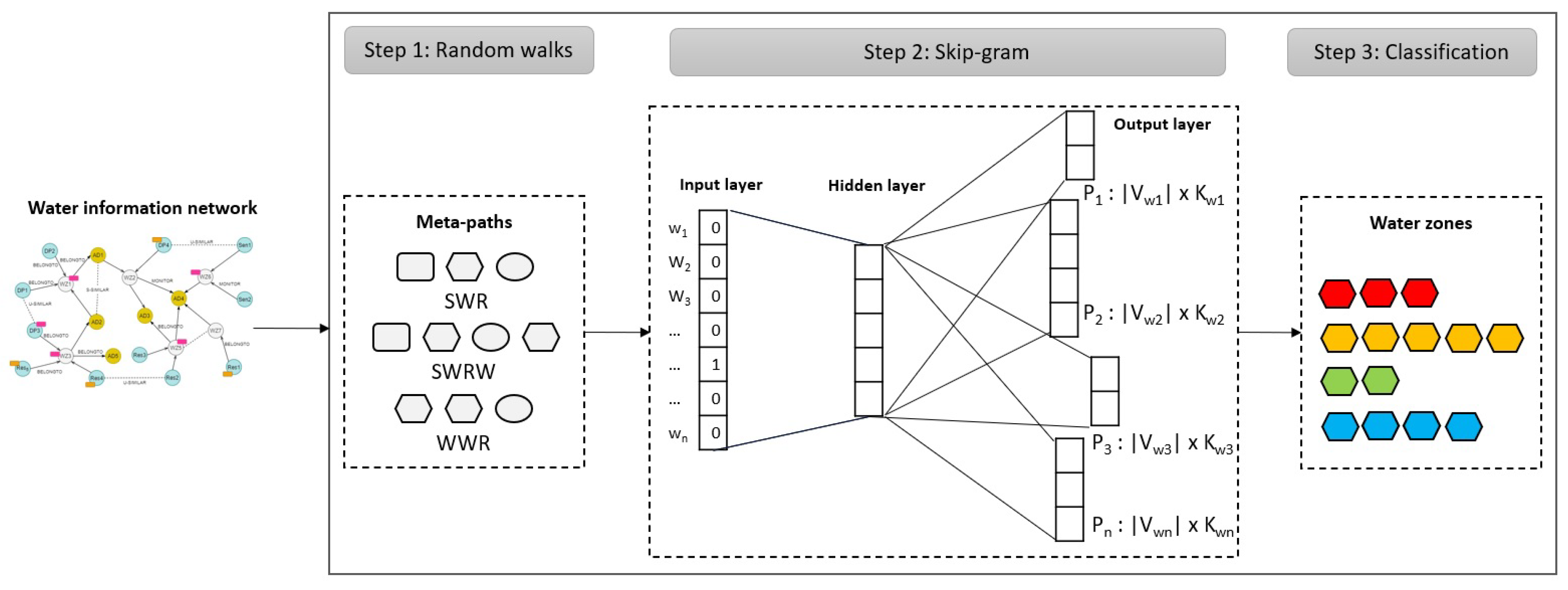
Inspired by metapath2vec, we propose a two-step incremental embedding method that maps the water network into a vector space, facilitating consequently the classification of water zones’ entities, as well as the decision task (see Figure 5). The embedding model is preceded by a guided random walk that allows extracting the node sequences as input to the Skip-Gram learning model. To correctly capture the semantics and structural relationships between the water network’s nodes and properly incorporate their heterogeneous neighborhood into Skip-Gram, the proposed model follows a metapath-guided random walk in the water network. The basic notations are presented in Table 4.
Meta-path-based random walks: In this work, a meta-path is a set of heterogeneous nodes which are connected based on their typed relations in the WKG. Formally, a meta-path P has the form e 1 r 1 e 2 r 2 e 3 r l 1 e l , wherein r = r 1 r 2 r l 1 denotes a composite relation between the node types e 1 and e l 
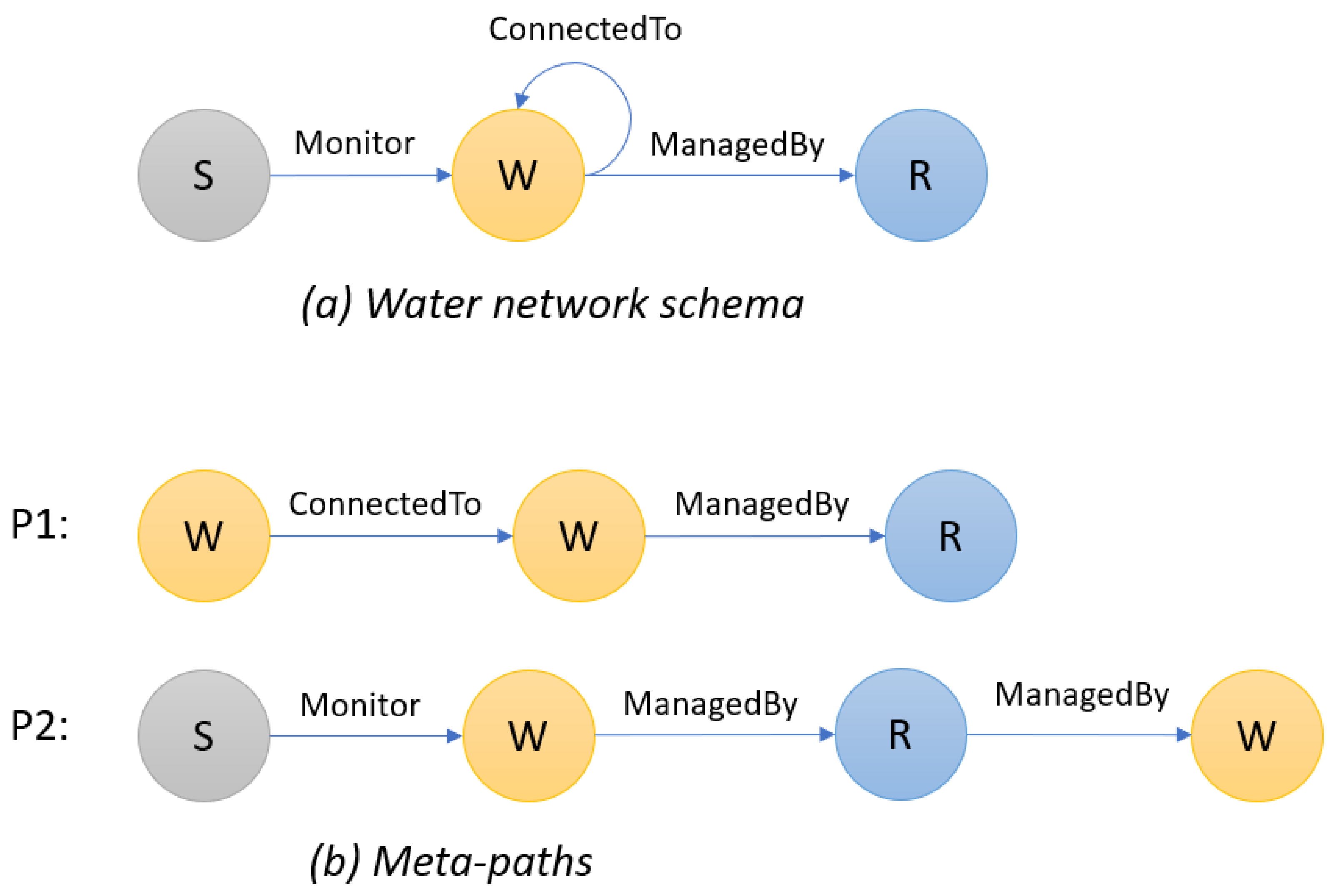
. The created meta-paths help training the Skip-Gram learning model, based on complex relations, such as water–water object relations (e.g., distribution pipeline, water reservoirs) and sensor–water object relations. Taking Figure 6 as example, the meta-path P : S-W-R denotes a management relationship between a water reservoir W being monitored by a sensor S and repaired using a management policy (e.g., repair) R. Two nodes from the same type can be connected via multiple meta-paths, e.g., E-S-E, and E-R-E. Each one reveals different semantics. For example, the latter meta-path indicates that a water zone’s management policy could be delivered for two water entities with similar behavior.
The meta-paths are used to recursively guide random walkers based on a transition probability, defined as follows [35]:
p ( v i + 1 | v t i , P ) = 1 | N t + 1 ( v t i ) | ( v i + 1 , v t i ) E , ( v i + 1 ) = t + 1 0 ( v i + 1 , v t i ) E , ( v i + 1 ) t + 1 0 ( v i + 1 , v t i ) E
Here, v t i V t and N t + 1 ( v t i ) denote, respectively, the node v of type t and its neighborhood type, which is outputted by the neighborhood function N t + 1 ( v t i ) , where v i + 1 V t + 1 . p ( v i + 1 | v t i , P ) = 0 , if the transition (v i + 1 , v i t ) does not exist in the set of edges E, or the neighbor node’s type is different from the expected node type given in the meta-path P .
The recursive guidance for the meta-path random walkers is defined as: p ( v i + 1 | v t i ) = p ( v i + 1 | v 1 i ) , if t = 1 . For example, the neighborhood of a water pipeline p 11 (see Figure 4) can be structurally close to other water entities (e.g., pipeline p 12 , reservoirs v 11 , v 13 ). Using the meta-path P : W-W-R, the random walkers could traverse the water network and incorporate the following node sequence into a neighborhood function: p 11 r 1 p 12 r 2 v 11 r 3 v 13 . Hence, given a water node and a predefined meta-path, the random walkers can determine the node representation that maximizes the probability of predicting an unseen node from a partially seen path in the water network.
The above guided random walk strategy preserves the semantic relationships between the types of nodes for each sequence, which leads to proper learning when these latter are incorporated into Skip-Gram.
Incremental embedding: As in the original metapath2vec, the water meta-paths are used as input to Skip-Gram. This latter is trained in order to obtain node (water objects) representations. The resultant node embeddings are frequently updated by taking into account the monitoring data, i.e., observations at each window time, due to the ever-changing nature of the water network. To do so, consider a set V = V + Δ V of the nodes whose states are changed after the monitoring task, where Δ is an increment denoting the amount of water network changes (e.g., pipeline removal, newly added reservoir, etc.). For example, a reservoir that is represented by the node v V may undergo a change in the water quality. In this case, v will represent the updated embedding for the node v.
To learn high-quality representations of the water network’s updated content, the model needs to maximize the likelihood of each water node to each context, as well as maximizing the probability that a context N t ( v ) ( v V , t T V ) is heterogeneous. Such probability is computed as follows [35]:
a r g m a x θ v V t T v c t N t ( v ) l o g p ( c t | v ; θ )
where N t ( v ) denotes the neighborhood of a water object v V , and l o g p ( c t | v ; θ ) is defined as a softmax function.
To efficiently predict each node’s neighborhood, the embedding model is based on a heterogeneous negative sampling strategy, in which a heterogeneous set of typed nodes is selected for the normalization and optimization of softmax function, w.r.t. the node context c t . Hence, given a typed node-set V t in the WKG and a node context c t , the softmax function is defined as follows:
p ( c t | v ; θ ) = e X c t . e X v u t V t e X u t . e X v
By considering the updates in the water network, the overall loss function is decomposed and defined as follows:
O ( X ) = l o g ( X c t . X v ) + m = 1 M E u t m P t ( u t ) [ l o g ( X u t m . X v ) ]
As in most approaches, the stochastic gradient descent (SGD) algorithm is used to optimize the embedding model.
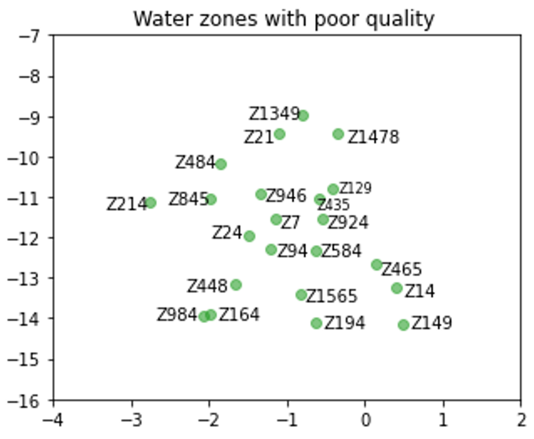
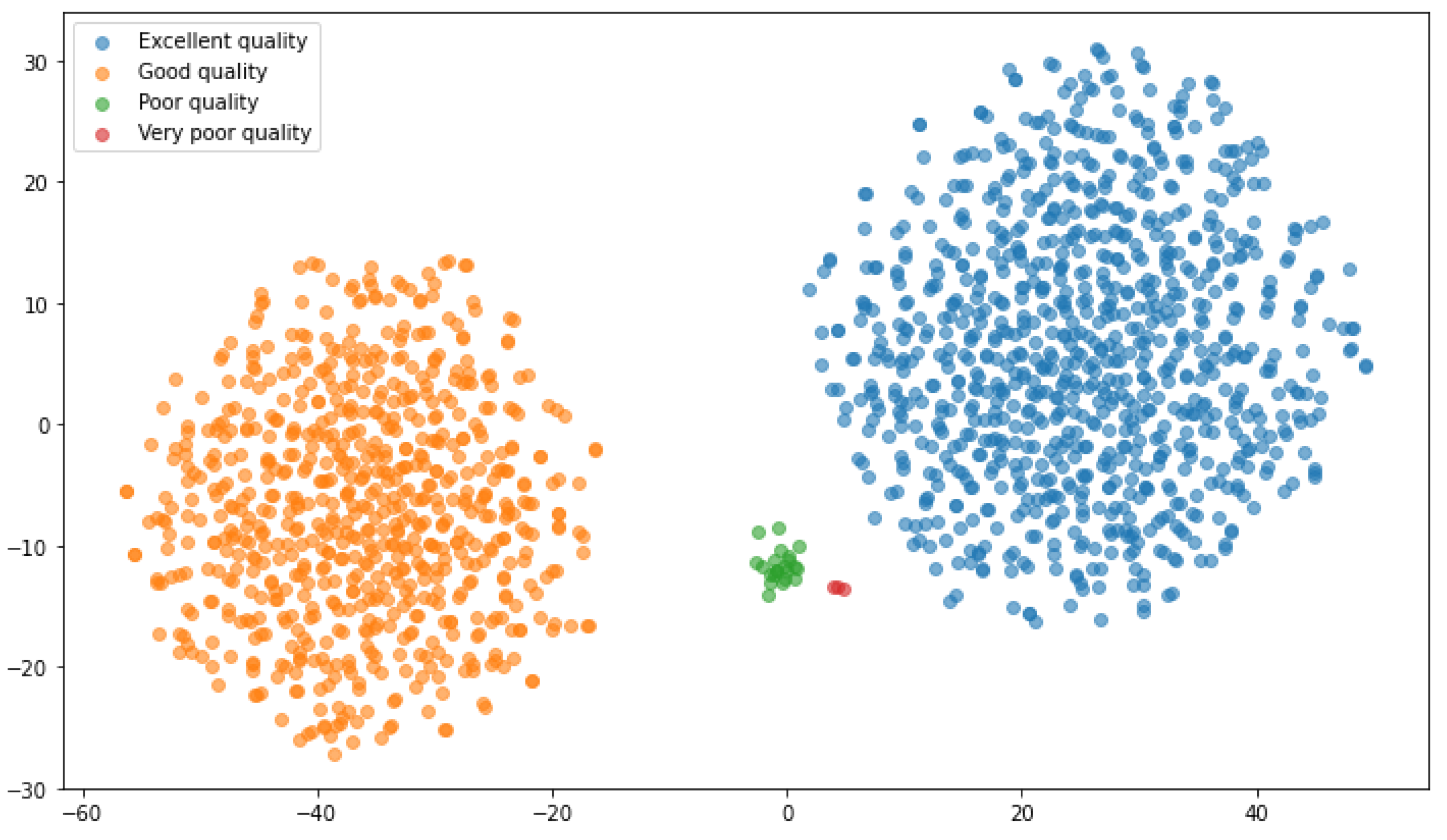
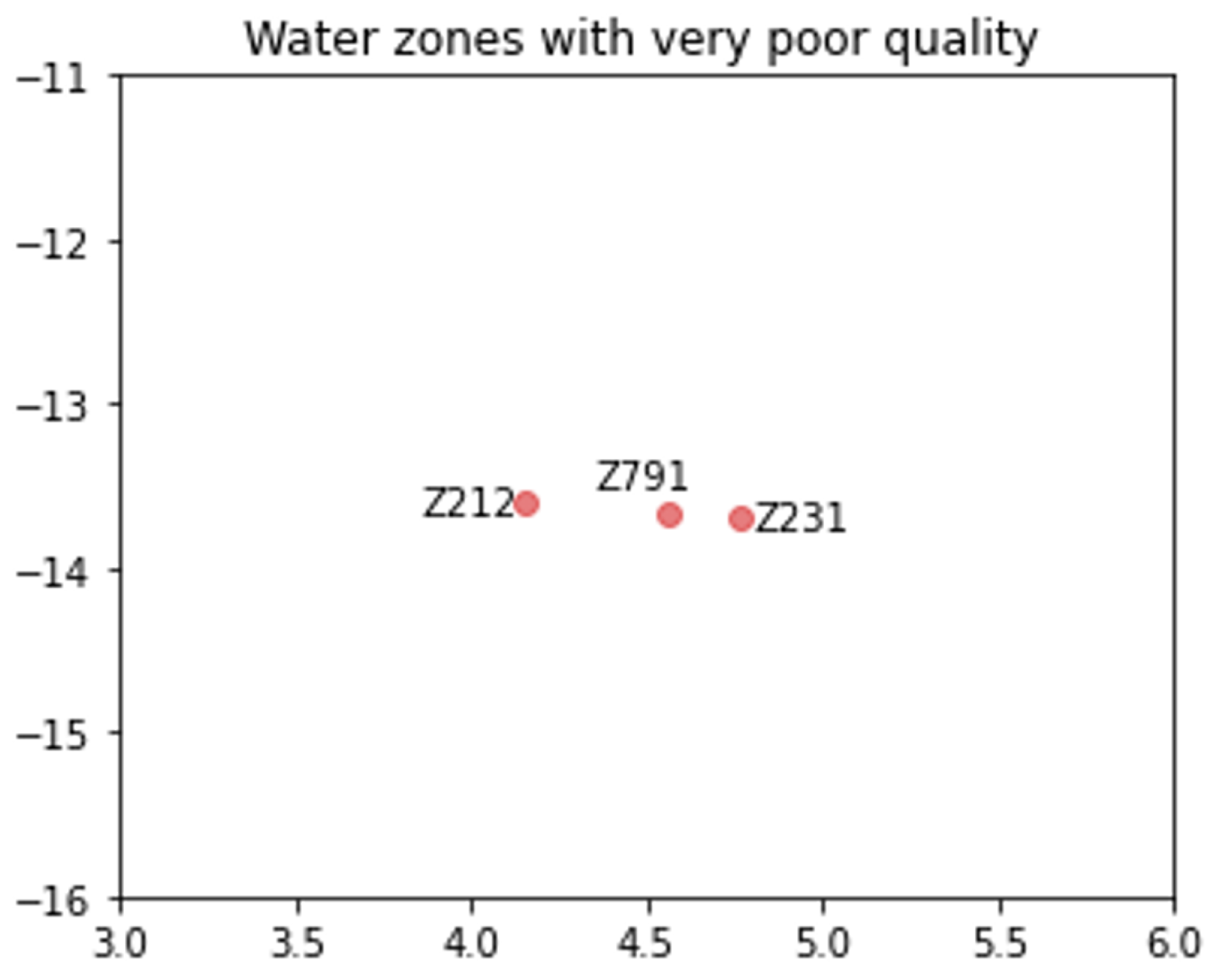
Classification of water zones based on incremental embedding: Based on the embeddings of the water network, and knowing that the water entities that share similar features or encounter the same deviations in their characteristics are close in the embedding space, the last step aims at inferring additional knowledge regarding the water zones, such as their quality (e.g., drinkable, pH level, etc.). By classifying the water network’s entities according to their proximity in the low-dimensional vector space, corrective measures will be triggered for each set of water objects, rather than selecting conflicting management actions for each individual water object. The correct decision on the water quality mainly depends on the accuracy of the learned embeddings in capturing the label of each water entity, based on the monitored data. In the embedding space, the water entities with similar behavior (indicated by the colored labels in Figure 4) are located closely, which facilitates their classification and, consequently, the selection of non-conflicting corrective measures.
The whole embedding and classification process is summarized in Algorithm 1.
Algorithm 1 Water zones’ embedding
 1:
Input: G —Water knowledge graph, L —Set of labels.
 2:
Output: V l p —Classification of node embeddings in the water network.
 3:
Begin
 4:
{ E t p } t = 1 T
 5:
for each node v i V  do
 6:
    X = MetaPathRandomWalk(G, P, v i , l)
 7:
    X = HeterogeneousSkipGram(X, k, M P );
 8:
    for each node type t T  do
 9:
        Learn the representations of node v i
10:
         L Minimize relation’s inference loss for v i
11:
         V l p V l p v i
12:
    end for
13:
end for
14:
Return { V l p } l = 1 | L |
Given a water network G and a finite set L of labels denoting the possible water states, Algorithm 1 determines, for each node v G , the set of sequences that result from the guided random walks with a length l (lines 5–6). Then, based on Skip-Gram, the node paths are incorporated into the neighborhood function (line 7). Finally, using the labels set L , the vectorized forms of each water entity are grouped using a classifier while minimizing the inference loss (lines 8–12).
The complexity of Algorithm 1 mainly depends on the meta-paths length ( l ) and the number of nodes ( | V | ) in the WIN. The guided random walks and the probability calculation based on Skip-Gram are iterated for each water node v i V . Then, these latter representations are determined by considering | T | node types. The complexity of this algorithm is of the order of O ( | V | . l 2 . | T | ) .

7. Decision Process

At this stage of the smart water surveillance process, the water zones with common abnormal behaviors (e.g., water quality degradation, turbidity, pipeline bursts, etc.) are repaired by triggering suitable management operations. Rather than running throughout the whole WIN, the decision mechanism exploits the groups of labeled nodes that resulted from the classification step (see 
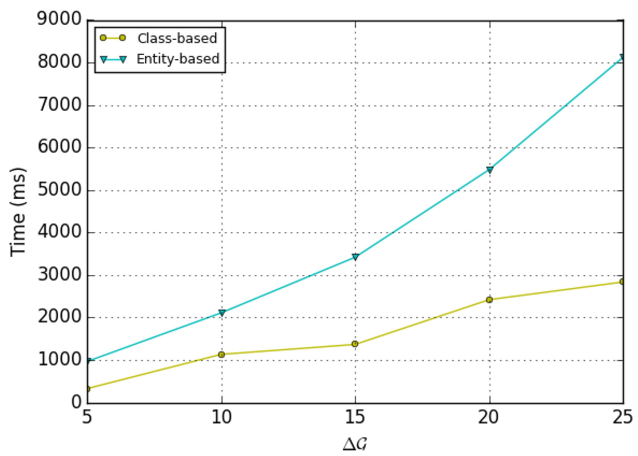
Section 6). Since each group of water entities that encounters the same problem (e.g., reservoirs leakage) is mapped into close vectors in the same embedding subspace, a unique management plan is generated for those affected water entities, avoiding then conflicts between corrective measures and reducing the decision complexity.
Knowing that each label denotes a triggering situation, an algorithm is defined in this work, to explore the embedding space and to locate the vectors representing the most appropriate water management actions for each class of water problem (e.g., leakage, high-pressure, etc.). Algorithm 2 takes, as input, the vectorized form of the updated labeled graph G , and outputs a set P of corrective measures.
Algorithm 2 Smart water decision-making
 1:
Input: W —Water knowledge graph, L p —Set of triggering events.
 2:
Output:P—Set of water management actions.
 3:
Begin
 4:
P
 5:
for l = 1 : L p do
 6:
    for each  w e W ( l )  do
 7:
        Locate w e in G
 8:
        for each action a i C o n t e x t ( w e ) do     ▹ Get management actions for the water entity w e
 9:
           if  < L p ( i ) , T r i g g e r , a i > W AND a i P then     ▹ Check the fact’s existence in W
10:
               add a i to P          ▹ Save corrective measure a i for the water entity w e
11:
           end if
12:
        end for
13:
    end for
14:
end for
15:
ReturnP
Based on a subset L p L of labels (line 5) denoting the classes of detected problems (triggering events), Algorithm 2 starts by locating the affected water entities W ( l ) for the water event l (lines 5–7). Then, for each one, its context is extracted (line 8) so that to evaluate the candidate water management operations. For each class l L p of problem, the suitable corrective measure is selected and saved to repair each water entity w e W ( l ) (line 10). Finally, a set P of water management operations is returned as the algorithm’s output (line 15).
The computational complexity of Algorithm 2 mainly depends on the number of triggering events ( | L p | ) and the water network’s size ( | V | ). The processing of each event requires parsing the WKG to locate the event context ( C ( w e ) ), including candidate management actions, which also need to be evaluated to select the best corrective measure. Hence, the whole decision process takes O ( | L p | . | V | . | C ( w e ) | ) .

8. Experiments

8.1. Dataset and Experimental Protocol

In this work, Google Colaboratory was used to encode the whole water management process with Python 3.7.12. The incremental embedding of the WIN was implemented using PyTorch: an open-source, flexible, and modular framework based on the Torch library. PyTorch Geometric (PyG) library was also used to enable a distributed and scaled representation of WIN entities. PyG provides a wide range of methods for deep learning on graphs, such as the creation and training of Graph Neural Networks (GNNs), and deals with irregular structures of input data, such as graphs and manifolds. The t-distributed stochastic neighbor embedding (t-SNE) library is also employed to project and visualize the water environment’s data and to reduce their dimensionality.
Experiments were conducted utilizing a dataset containing water quality data from several locations to evaluate the proposed approach, briefly called SWM-INRL (Smart Water Management with Incremental NRL). This dataset contains a total of 1600 samples with 9 parameters: temperature, pH, turbidity, Dissolved Oxygen (DO), conductivity, Biological Oxygen Demand (BOD), Nitrate (NI), Fecal Coliform (FC), and Total Coliforms (TC). Since the dataset lacked triggering events and their associated conditions, this information was added based on the case of water quality, by computing the Water Quality Index (WQI) and classifying water samples based on the WQI values. WQI has been calculated using the following formula [47]:
W Q I = j = 1 N q j w j j = 1 N w j
where N is the total number of parameters included to compute the WQI, q j presents the quality rating scale of the used parameters calculated through Equation (6), and w j is the unit weight of the used parameters calculated by Equation (7).
q j = v j v p e r f e c t r v j v p e r f e c t 100
where v j is the measured value of the jth parameter for each station, v p e r f e c t is the perfect value of the jth parameter in case of a good quality of water, and r v j is the recommended value for this parameter. Since perfect values are rarely available in real water environments, the recommended values are the standard values determined by the WHO. The perfect and recommended values for each parameter are as follows: p H {7,8.5}, t u r b i d i t y {0,5}, D O {14.6,10}, c o n d u c t i v i t y {0,1000}, B O D {0,5}, N I {0,45}, F C {0,100}, T C {0,1000}.
w j = K r v j
where K is the proportionality constant calculated using Equation (8):
K = 1 j = 1 N r v j
Table 5 depicts the four classes of water quality and their distribution added to the considered dataset, namely Excellent with a WQI range of less than 25, Good with a WQI range in [26, 50], Poor with a WQI range in [51, 75], and Very poor with a WQI range greater than 75. Table 6 shows a sample from the water dataset with different measures of the nine parameters used to identify the water quality.
The WKG was built as an information network with three sorts of nodes: water zone, event, and action. The location IDs are extracted to represent the water entities, while the changes in WQI for each water zone are used to represent the event entities. For the actions, the entities representing the management policies were randomly generated. The relationships among these entities represent the topology of the water network. In addition, the water zone and event nodes are labeled to present the quality of water according to WQI values. To continuously update the WKG structure, metapath2vec implementation was applied and the model was configured according to the setting and hyper-parameters depicted in Table 7. The P : W-E-C-E-W was defined as the guided meta-path followed to generate the random walks. In fact, W-E-C-E-W represents the heterogeneous semantic of water zones that have events belonging to the same class.
Since some entities may feature the same behavior or deviation, our idea is to trigger a corrective action for a group of water entities, not for a single entity. That has several advantages: (i) reducing the complexity of processing each water entity in isolation (ii) unifying water management policies to avoid incompatibility and conflicts between them. For this purpose, we opted for the classification of water zones according to their water quality levels. By this way, a poor quality situation, for example, will trigger the same corrective action for all the low-quality water zones. In the current version, for simplicity reasons, we focused on the classes of water quality degradation, based on 9 water features, while the other triggering events, such as pressure loss, chlorination, leakage, etc. (see Table 2), will be considered in a more complete version of our smart water management system. This will be achieved by incorporating additional features of various water entities into the water knowledge graph, as well as the embedding and classification model.

8.2. Experimental Results

8.2.1. Water Zones Embedding Visualization

To capture semantic and structural correlations between different zone locations, the proposed SWM-INRL approach is based on metapath2vec, as an incremental embedding technique, as previously mentioned. Figure 7 visualizes the latent vectors learned by metapath2vec model of 1600 water zones. It is clear that the water zones with similar characteristics are classified (see Section 8.2.2) and grouped to each other. They also were separated from other nodes according to the water quality.
As can be noticed, most of the water zones belong to the excellent and good water quality classes (54.98%, 43.49%, 1.35%, 0.18%, for excellent, good, poor, and very poor, respectively).
Figure 8 and Figure 9 depict respectively the water zones with poor and very poor water quality.

8.2.2. Water Zones Classification

This section’s goal is to compare the performance of water zone classification with and without embedding. To do this, three classifiers are considered: Support Vector Machines (SVM), Logistic Regression (LR), and K-Nearest Neighbors (KNN). The node representations are learned from the dataset, which was transformed into a knowledge graph. The embeddings of the above-labeled nodes are then fed into the classifiers. Classification results, based on the 9 parameters of the dataset (see Section 8.1), are presented in Table 7 and Table 8. Confusion matrices of the three classifiers SVM, LR, and KNN according to the four classes (excellent, good, poor, and very poor) are depicted in Figure 10 and Figure 11. It is noticed that the SVM classifier outperforms other classifiers for both cases (with and without embedding). Furthermore, adopting incremental network embedding improved classification scores for all three classifiers by at least 3%. The results prove the role of latent representations learned by embedding for a correct water zone classification. The metapath2vec model has a solid ability to generate appropriate embeddings for the WIN.

8.3. Evaluation of NRL-Based Method

8.3.1. Comparison of Classification Accuracy

The goal of these test series is to evaluate the ability of the proposed approach to correctly classify the water zones’ entities, which is essential to trigger the appropriate corrective measures. We also leverage the importance of incremental learning in mapping water entities with similar behavior into close vector representations, which facilitates their classification. For this purpose, tests were conducted with three different classifiers (SVM, LR, and KNN). After that, the same tests were repeated without executing the incremental embedding step. For all the compared methods, the number of water entities was set to 1600 and the number of classes, i.e., water quality deviations, to 4. Results are recorded in Figure 12, Table 8 and Table 9.
Figure 12 shows that the proposed approach performs better with the incremental learning step and outperforms the traditional classification methods. Regardless of the applied classifier, the gap in accuracy results reached 3 % with the S V M classifier. It is worth noting that the used dataset is with an imbalanced classes distribution, as depicted in Table 5. Nevertheless, we conclude from the obtained results that modeling the water environment as a knowledge graph and exploiting network embedding have effectively dealt with the imbalanced distribution of each class. In fact, the incremental embedding helps learn semantics and rich representations, hence mapping the water entities as close as possible in the embedding space, according to their similar features, behaviors, and deviations. Therefore, the learned representations will be useful to correctly classify water entities. The classification with embedding achieved high performance and outperformed the traditional classification methods. Indeed, the guided random walk technique used in the present work aided in the preservation of the semantic relationships between the water network content, i.e., nodes for each sequence. This increased the possibility of each water node fitting into each context, resulting in accurate learning of water entity vector forms. As a result, water zones with similar characteristics (e.g., volume, water quality) and experiencing the same anomalous behavior will be close in the embedding space and belong to the same class.

8.3.2. Computational Complexity

The goal of this test series is to study the time complexity of SWM-INRL by considering the amount of captured changes at each water zone (variation of Δ in [5%, 10%, 15%, 20%, 25%). For each test case, the computation time was recorded at both the water entity level and the water class level. The recorded results in Figure 13 are computed as the sum of incremental embedding time ( T E ), the time devoted to exploring the embedding space for the classification purpose ( T C ), and the time spent to select a management operation for a water zone’s critical case ( T D ).
It is evident from Figure 13 that SWM-INRL performs better when the decision is taken for each class of problem (e.g., leakage, pressure loss) rather than for each affected water entity. This ascertainment is understandable because the decision routine is not repeated for a high number of separate water zones, which will cause extra-computation time. Thanks to the incremental embedding, the affected water zones were mapped into close vector representations according to their common deviations, which transformed the decision task from a water entity-oriented recommendation to a class-oriented recommendation. Regardless of the amount of captured changes ( Δ G ), running through a traditional graph-like water network requires the processing of each water entity, even those that feature a stable state, which increases the total time of the measure-decide-actuate process. This gap in processing time can be clearly seen from Figure 13, and has reached 5.287 s when 25% of the water zones have encountered abnormal behavior. Unlike the traditional graph processing approach, the proposed NRL-based method transforms the whole WIN into clusters, where the largest one (see Figure 7), which represents the stable water zones, will not be treated by the decision algorithm. By this way, the decision process will be limited to a small number of clusters (e.g., 2 clusters in Figure 7), denoting the affected water zones. That positively impacts the total execution time, especially in a more complex and highly dynamic ( Δ ) water network.

9. Discussion

In a context of increasing scarcity of water resources and an increasingly demanding regulatory framework, organizations concerned with the management of water resources, government authorities, and drinking water operators, both public and private, are facing today growing and complex challenges: monitoring water quality, improving the efficiency of water networks, reducing operating costs, improving energy performance, etc. The growth of IoT sensors, the deployment of efficient and intelligent networks for data transfer, the usage of artificial intelligence, and notably machine learning techniques, are all highlighted as challenges that intelligent network management approaches can tackle. In this context, the solution consisted in a novel IoT-based framework for smart monitoring of water environments. The proposed framework relies mainly on the knowledge graph embedding technique that will enable us to progressively learn the semantics and enrich representations of water entities modeled in the form of a knowledge graph and map them into a low-dimensional vector space, according to their characteristics, behaviors, and deviations. This technique makes it possible to classify water entities to detect abnormalities that require effective and urgent intervention to select and initiate appropriate corrective measures.
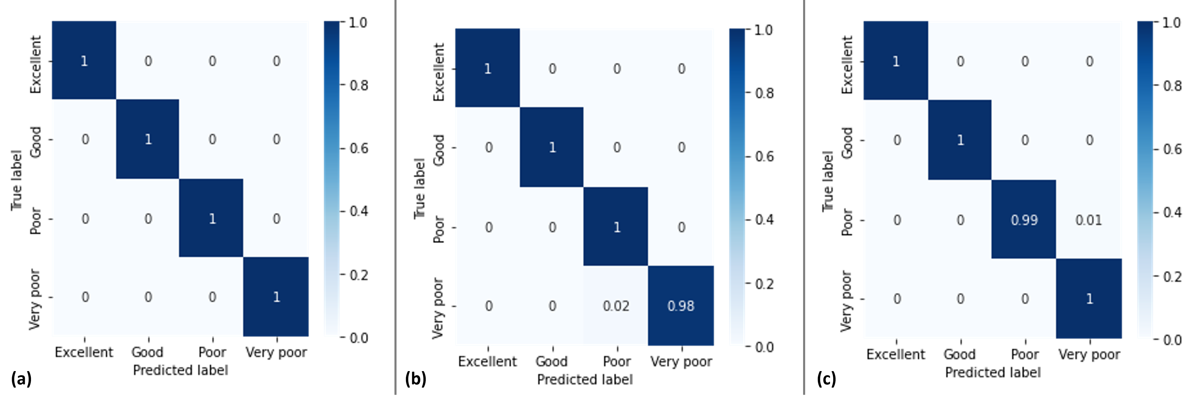
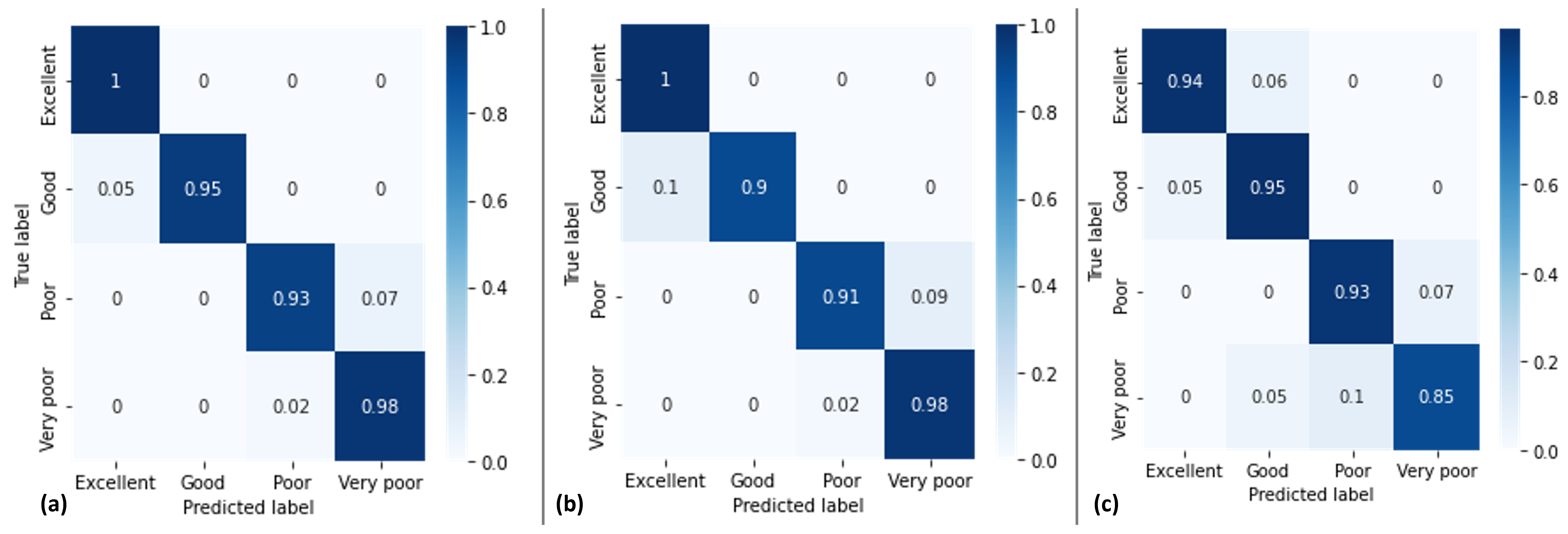
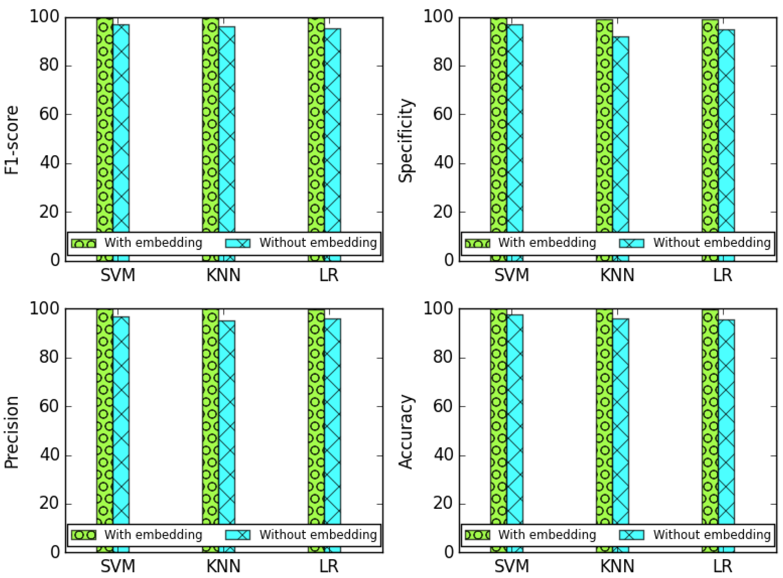
The experimental studies that were carried out in this work confirmed that the adoption of Knowledge Graph Embedding (KGE) improved the performance of the water management task and the decision-making process. In fact, KGE is usually performed as a step that precedes several downstream tasks (e.g., classification, clustering, anomaly detection, link prediction, etc.) in order to improve the system’s performance and quality [14]. In this paper, the main goal was to classify water entities in order to reduce the complexity and cost of decision-making. Since the incremental learning of the water network representation made it possible to map the water entities in close vectorized forms, advanced management operations could be efficiently carried out. For example, the anomaly detection problem could be instantiated as part of water management to determine areas of water exhibiting abnormal behavior. These will be isolated since they do not share the same semantics with the rest of the water entities. Another management operation concerns reassigning surveillance actors, such as sensors and their associated services (e.g., sensor cloud services, micro-services), to manage water areas. In fact, some areas may be characterized by a high degree of change in the water quality, while other areas that do not undergo frequent changes will produce a few amounts of water change-related data. In such a situation, embedding the water network will better capture the semantics by factoring the scattered water data into a smooth embedding space. In this way, high-performance sensors will be placed in tight water areas with a high degree of change, making it easier to reconfigure their placement.
In addition to the previously mentioned advantages and applicability cases, in the case of water resource management systems, the adoption of knowledge graph integration can overcome the limitations of usual deep reinforcement learning-based systems [48,49]. The deployment of this type of water management systems requires a huge amount of information from IoT sensors. However, knowledge reasoning techniques can solve this problem by using a graph already constructed on prior knowledge of the entities’ correlation and employing integration to derive the correct classification—subsequently, the effective selection of the appropriate corrective actions.

10. Conclusions

In this paper, a novel IoT-based framework was proposed to allow controlling water quality and to optimize drinking water consumption through a set of intelligent corrective measures and management policies. By combining the strengths of knowledge graph technology [13] and NRL [14,15], the knowledge graph-like WIN incrementally mapped into a low-dimensional vector space that is continuously readjusted to take into account the detected changes/problems in the monitored water zones. The motivation behind the incremental embedding step is to facilitate the decision on the appropriate management action through the classification and grouping of affected water zones. The experimental studies with a real-world water dataset proved that the proposed SWM-INRL solution could provide efficient monitoring and management facilities for organizations in both the public and private sectors to ensure high-quality water resources and services. The experiments have also proven that the incremental learning method reduced this complexity by exploring a vector subspace of infected water entities rather than exploring the large WIN. Hence, increasing the accuracy of locating the affected water zones and their related management policies.
The present work will be improved by learning the representation of the water network under uncertainty of water information, which will offer probabilistic and predictive capacities to the monitoring system. The future work will also be focused on investigating the impact of correlating water KPIs on the final analytics results [29]. In addition, spatial time-series forecasting techniques will be explored to tackle the scalability problem caused by processing complex and large amounts of data collected by IoT networks [50]. Finally, future extensions will also include the integration of ontological properties of water resources and observation data to take advantage of assets offered by existing ontologies used in the smart water domain [51].

Author Contributions

Conceptualization, H.M., M.D. and W.B.; methodology, H.M., M.D. and W.B.; validation, W.B. and S.B.A.; formal analysis, H.M., M.D. and W.B.; investigation, H.M. and M.D.; resources, H.M. and M.D.; data curation, W.B. and S.B.A.; writing—original draft preparation, H.M., M.D., W.B. and S.B.A.; writing—review and editing, H.M., M.D., W.B., S.B.A., M.S. and N.A.; visualization, H.M., M.D., W.B. and S.B.A.; supervision, H.M., M.D. and W.B. All authors have read and agreed to the published version of the manuscript.

Funding

This research was funded by the Deputyship for Research & Innovation, Ministry of Education in Saudi Arabia under the project number (442/210).

Acknowledgments

The authors extend their appreciation to the Deputyship for Research & Innovation, Ministry of Education in Saudi Arabia for funding this research work; project number (442/210). Also, the authors would like to extend their appreciation to Taibah University for its supervision support.

Conflicts of Interest

The authors declare no conflict of interest.

References

  1. Water Scarcity. Available online: https://www.worldwildlife.org/threats/water-scarcity (accessed on 6 August 2021).
  2. WHO Guidelines for Drinking-Water Quality. Available online: https://apps.who.int/iris/bitstream/handle/10665/254637/9789241549950-eng.pdf (accessed on 6 August 2021).
  3. Water Quality Criteria. Available online: https://www.epa.gov/wqc (accessed on 21 December 2021).
  4. Abba, S.; Hadi, S.J.; Sammen, S.S.; Salih, S.Q.; Abdulkadir, R.; Pham, Q.B.; Yaseen, Z.M. Evolutionary computational intelligence algorithm coupled with self-tuning predictive model for water quality index determination. J. Hydrol. 2020, 587, 124974. [Google Scholar] [CrossRef]
  5. Mirzaei, M.; Jafari, A.; Gholamalifard, M.; Azadi, H.; Shooshtari, S.J.; Moghaddam, S.M.; Gebrehiwot, K.; Witlox, F. Mitigating environmental risks: Modeling the interaction of water quality parameters and land use cover. Land Use Policy 2020, 95, 103766. [Google Scholar] [CrossRef]
  6. Asadollah, S.B.H.S.; Sharafati, A.; Motta, D.; Yaseen, Z.M. River water quality index prediction and uncertainty analysis: A comparative study of machine learning models. J. Environ. Chem. Eng. 2021, 9, 104599. [Google Scholar] [CrossRef]
  7. Deng, T.; Chau, K.W.; Duan, H.F. Machine learning based marine water quality prediction for coastal hydro-environment management. J. Environ. Manag. 2021, 284, 112051. [Google Scholar] [CrossRef] [PubMed]
  8. Butler, D.; Ward, S.; Sweetapple, C.; Astaraie-Imani, M.; Diao, K.; Farmani, R.; Fu, G. Reliable, resilient and sustainable water management: The Safe & SuRe approach. Glob. Chall. 2017, 1, 63–77. [Google Scholar] [PubMed]
  9. Vocciante, M.; Bagatin, R.; Ferro, S. Enhancements in electrokinetic remediation technology: Focus on water management and wastewater recovery. Chem. Eng. J. 2017, 309, 708–716. [Google Scholar] [CrossRef]
  10. Atitallah, S.B.; Driss, M.; Boulila, W.; Ghézala, H.B. Leveraging Deep Learning and IoT big data analytics to support the smart cities development: Review and future directions. Comput. Sci. Rev. 2020, 38, 100303. [Google Scholar] [CrossRef]
  11. Driss, M.; Hasan, D.; Boulila, W.; Ahmad, J. Microservices in IoT Security: Current Solutions, Research Challenges, and Future Directions. arXiv 2021, arXiv:2105.07722. [Google Scholar] [CrossRef]
  12. Latif, S.; Driss, M.; Boulila, W.; Jamal, S.S.; Idrees, Z.; Ahmad, J. Deep Learning for the Industrial Internet of Things (IIoT): A Comprehensive Survey of Techniques, Implementation Frameworks, Potential Applications, and Future Directions. Sensors 2021, 21, 7518. [Google Scholar] [CrossRef]
  13. Ji, S.; Pan, S.; Cambria, E.; Marttinen, P.; Philip, S.Y. A survey on knowledge graphs: Representation, acquisition, and applications. IEEE Trans. Neural Netw. Learn. Syst. 2021, 33, 494–514. [Google Scholar] [CrossRef]
  14. Zhang, D.; Yin, J.; Zhu, X.; Zhang, C. Network representation learning: A survey. IEEE Trans. Big Data 2018, 6, 3–28. [Google Scholar] [CrossRef] [Green Version]
  15. Li, B.; Pi, D. Network representation learning: A systematic literature review. Neural Comput. Appl. 2020, 32, 16647–16679. [Google Scholar] [CrossRef]
  16. Singh, M.; Ahmed, S. IoT based smart water management systems: A systematic review. Mater. Today Proc. 2021, 46, 5211–5218. [Google Scholar] [CrossRef]
  17. Jan, F.; Min-Allah, N.; Düştegör, D. IoT Based Smart Water Quality Monitoring: Recent Techniques, Trends and Challenges for Domestic Applications. Water 2021, 13, 1729. [Google Scholar] [CrossRef]
  18. Park, J.; Kim, K.T.; Lee, W.H. Recent advances in information and communications technology (ICT) and sensor technology for monitoring water quality. Water 2020, 12, 510. [Google Scholar] [CrossRef] [Green Version]
  19. Driss, M.; Aljehani, A.; Boulila, W.; Ghandorh, H.; Al-Sarem, M. Servicing your requirements: An fca and rca-driven approach for semantic web services composition. IEEE Access 2020, 8, 59326–59339. [Google Scholar] [CrossRef]
  20. Ranjithkumar, M.; Robert, L. Machine Learning Techniques and Cloud Computing to Estimate River Water Quality—Survey. In Inventive Communication and Computational Technologies; Springer: Berlin/Heidelberg, Germany, 2021; pp. 387–396. [Google Scholar]
  21. Driss, M.; Atitallah, S.B.; Albalawi, A.; Boulila, W. Req-WSComposer: A novel platform for requirements-driven composition of semantic web services. J. Ambient. Intell. Humaniz. Comput. 2021, 1–17. [Google Scholar] [CrossRef]
  22. Salam, A. Internet of Things for Sustainable Community Development; Springer: Berlin/Heidelberg, Germany, 2020. [Google Scholar]
  23. Prasad, A.; Mamun, K.A.; Islam, F.; Haqva, H. Smart water quality monitoring system. In Proceedings of the 2015 2nd Asia-Pacific World Congress on Computer Science and Engineering (APWC on CSE), Nadi, Fiji, 2–4 December 2015; pp. 1–6. [Google Scholar]
  24. Shahanas, K.M.; Sivakumar, P.B. Framework for a smart water management system in the context of smart city initiatives in India. Procedia Comput. Sci. 2016, 92, 142–147. [Google Scholar] [CrossRef] [Green Version]
  25. Goel, D.; Chaudhury, S.; Ghosh, H. Smart water management: An ontology-driven context-aware IoT application. In Proceedings of the International Conference on Pattern Recognition and Machine Intelligence, Kolkata, India, 5–8 December 2017; Springer: Berlin/Heidelberg, Germany, 2017; pp. 639–646. [Google Scholar]
  26. Myint, C.Z.; Gopal, L.; Aung, Y.L. Reconfigurable smart water quality monitoring system in IoT environment. In Proceedings of the 2017 IEEE/ACIS 16th International Conference on Computer and Information Science (ICIS), Wuhan, China, 24–26 May 2017; pp. 435–440. [Google Scholar]
  27. Simmhan, Y.; Ravindra, P.; Chaturvedi, S.; Hegde, M.; Ballamajalu, R. Towards a data-driven IoT software architecture for smart city utilities. Softw. Pract. Exp. 2018, 48, 1390–1416. [Google Scholar] [CrossRef]
  28. Mukta, M.; Islam, S.; Barman, S.D.; Reza, A.W.; Khan, M.S.H. IoT based smart water quality monitoring system. In Proceedings of the 2019 IEEE 4th International Conference on Computer and Communication Systems (ICCCS), Singapore, 23–25 February 2019; pp. 669–673. [Google Scholar]
  29. Liu, P.; Wang, J.; Sangaiah, A.K.; Xie, Y.; Yin, X. Analysis and prediction of water quality using LSTM deep neural networks in IoT environment. Sustainability 2019, 11, 2058. [Google Scholar] [CrossRef] [Green Version]
  30. Mamun, K.; Islam, F.; Haque, R.; Khan, M.G.; Prasad, A.; Haqva, H.; Mudliar, R.R.; Mani, F.S. Smart water quality monitoring system design and KPIs analysis: Case sites of fiji surface water. Sustainability 2019, 11, 7110. [Google Scholar] [CrossRef] [Green Version]
  31. Wang, X.; Wei, H.; Chen, N.; He, X.; Tian, Z. An Observational Process Ontology-Based Modeling Approach for Water Quality Monitoring. Water 2020, 12, 715. [Google Scholar] [CrossRef] [Green Version]
  32. Wybrands, M.; Frohmann, F.; Andree, M.; Gómez, J.M. WISdoM: An Information System for Water Management. In Advances and New Trends in Environmental Informatics; Springer: Berlin/Heidelberg, Germany, 2021; pp. 131–146. [Google Scholar]
  33. Carey, C.C.; Woelmer, W.M.; Lofton, M.E.; Figueiredo, R.J.; Bookout, B.J.; Corrigan, R.S.; Daneshmand, V.; Hounshell, A.G.; Howard, D.W.; Lewis, A.S.; et al. Advancing lake and reservoir water quality management with near-term, iterative ecological forecasting. Inland Waters 2021, 1–14. [Google Scholar] [CrossRef]
  34. Lloret, J.; García, L.; Jimenez, J.M.; Sendra, S.; Lorenz, P. Cluster-Based Communication Protocol and Architecture for a Wastewater Purification System Intended for Irrigation. IEEE Access 2021, 9, 142374–142389. [Google Scholar] [CrossRef]
  35. Dong, Y.; Chawla, N.V.; Swami, A. metapath2vec: Scalable representation learning for heterogeneous networks. In Proceedings of the 23rd ACM SIGKDD International Conference on Knowledge Discovery and Data Mining, Halifax, NS, Canada, 13–17 August 2017; pp. 135–144. [Google Scholar]
  36. Boulila, W.; Al-Kmali, M.; Farid, M.; Mugahed, H. A business intelligence based solution to support academic affairs: Case of Taibah University. Wirel. Netw. 2018, 1–8. [Google Scholar] [CrossRef]
  37. Chen, X.; Jia, S.; Xiang, Y. A review: Knowledge reasoning over knowledge graph. Expert Syst. Appl. 2020, 141, 112948. [Google Scholar] [CrossRef]
  38. Sun, S. A survey of multi-view machine learning. Neural Comput. Appl. 2013, 23, 2031–2038. [Google Scholar] [CrossRef]
  39. The Facts about Nutrient Pollution. Available online: https://www.epa.gov/nutrientpollution (accessed on 21 December 2021).
  40. Babu Loganathan, G.; Mohan, E.; Siva Kumar, R. Iot Based Water and Soil Quality Monitoring System. Int. J. Mech. Eng. Technol. (IJMET) 2019, 10, 537–541. [Google Scholar]
  41. Vinod, G.; Peter, A.; Rao, I.; Babu, Y. IoT based Water Quality Monitoring System Using WSN. Indian J. Public Health Res. Dev. 2018, 9, 1575–1578. [Google Scholar] [CrossRef]
  42. Agudelo-Vera, C.; Avvedimento, S.; Boxall, J.; Creaco, E.; de Kater, H.; Di Nardo, A.; Djukic, A.; Douterelo, I.; Fish, K.E.; Iglesias Rey, P.L.; et al. Drinking water temperature around the globe: Understanding, policies, challenges and opportunities. Water 2020, 12, 1049. [Google Scholar] [CrossRef] [Green Version]
  43. Vallino, E.; Ridolfi, L.; Laio, F. Measuring economic water scarcity in agriculture: A cross-country empirical investigation. Environ. Sci. Policy 2020, 114, 73–85. [Google Scholar] [CrossRef]
  44. Edition, F. Guidelines for drinking-water quality. WHO Chron. 2011, 38, 104–108. [Google Scholar]
  45. Abdul Haseeb-ur rehman, R.M.; Liaqat, M.; Aman, A.H.M.; Ab Hamid, S.H.; Ali, R.L.; Shuja, J.; Khan, M.K. Sensor Cloud Frameworks: State-of-the-Art, Taxonomy, and Research Issues. IEEE Sens. J. 2021, 21, 22347–22370. [Google Scholar] [CrossRef]
  46. Ali, I.; Ahmedy, I.; Gani, A.; Talha, M.; Raza, M.A.; Anisi, M.H. Data collection in sensor-cloud: A systematic literature review. IEEE Access 2020, 8, 184664–184687. [Google Scholar] [CrossRef]
  47. Aldhyani, T.H.; Al-Yaari, M.; Alkahtani, H.; Maashi, M. Water quality prediction using artificial intelligence algorithms. Appl. Bionics Biomech. 2020, 2020, 6659314. [Google Scholar] [CrossRef]
  48. Hajgató, G.; Paál, G.; Gyires-Tóth, B. Deep Reinforcement Learning for Real-Time Optimization of Pumps in Water Distribution Systems. J. Water Resour. Plan. Manag. 2020, 146, 04020079. [Google Scholar] [CrossRef]
  49. Mullapudi, A.; Lewis, M.J.; Gruden, C.L.; Kerkez, B. Deep reinforcement learning for the real time control of stormwater systems. Adv. Water Resour. 2020, 140, 103600. [Google Scholar] [CrossRef]
  50. Monteiro, M.; Costa, M. A time series model comparison for monitoring and forecasting water quality variables. Hydrology 2018, 5, 37. [Google Scholar] [CrossRef] [Green Version]
  51. Howell, S.; Beach, T.; Rezgui, Y. Robust requirements gathering for ontologies in smart water systems. Requir. Eng. 2021, 26, 97–114. [Google Scholar] [CrossRef]
Figure 1. Layered model of the smart water monitoring framework.
Remotesensing 14 00922 g001
Figure 2. System workflow of the smart water management process.
Remotesensing 14 00922 g002
Figure 3. Water knowledge graph.
Remotesensing 14 00922 g003
Figure 4. Updated WIN after the monitoring phase.
Remotesensing 14 00922 g004
Figure 5. Incremental embedding of the water network.
Remotesensing 14 00922 g005
Figure 6. A simple water network schema and two possible meta-paths in the water network.
Remotesensing 14 00922 g006
Figure 7. Embedding visualization of the constructed WKG.
Remotesensing 14 00922 g007
Figure 8. Water zones with poor quality.
Remotesensing 14 00922 g008
Figure 9. Water zones with very poor quality.
Remotesensing 14 00922 g009
Figure 10. Normalized confusion matrices for the water zones’ embedding classification with: (a) SVM, (b) LR, (c) KNN.
Remotesensing 14 00922 g010
Figure 11. Normalized confusion matrices for the water zones’ classification without embedding using: (a) SVM, (b) LR, (c) KNN.
Remotesensing 14 00922 g011
Figure 12. Comparison of the classification quality with and without incremental embedding.
Remotesensing 14 00922 g012
Figure 13. Computation time with different amounts of changes.
Remotesensing 14 00922 g013
Table 1. Examples of water quality sensors.
SensorDescriptionMeasured KPIRange
TemperatureSensor with no calibrationIt ensures the measurement of water temperature that has a substantial impact on water quality [42]. The WHO recommends a maximum temperature of 30 degrees Celsius for drinking water.−5 to 50 °C
pH / ORPOptional ORP sensor is combined with pH sensorIt measures water-based solution’s acidic and basic properties. A basic solution has a higher pH value, whereas an acidic solution has a lower pH value. WHO [43] suggests a pH range of 6.5–9.5 for optimum quality.0 to 14 units / −999 to 999 mV
TurbidityFiltered for non-turbidity spikes; includes wiper to clean the opticsThis sensor measures the turbidity metric, which is used for determining the clarity of water. It is a crucial indicator of water quality. It is usually measured in Formazin Turbidity Unit (FTU) or Nephelometric Turbidity Unit (NTU) (NTU). The value of turbidity in drinking water should be less than 5 NTU, according to WHO rules [44].0 to 1000 FNU 1000 to 4000 FNU
Total Dissolved Oxygen (TDO)Optical sensor compensated for temperature and salinityIt measures how much organic and inorganic material is dissolved in water. The presence of a substantial number of minerals is indicated by high TDS levels. TDO in drinking water should not exceed 500 mg/L. Water with a TDO level of more than 1000 mg/L is unsuitable for drinking.0 to 500% saturation
PressureCompensated for temperature, salinity, barometric pressure included with depth sensorPump rate and pressure affect the flow of drinking water. Water pressure sensors are used to determine the amount of water in a tank, as well as the rate at which that level changes. They can also be used to automatically decide whether pumps should be activated to increase the flow rate in pumps where water is flowing. Vented depth in [0, 10] m, Total dissolved gas in [400, 900] mm Hg
Table 2. Examples of corrective actions for water quality management.
EventConditionAction
Leakage, contaminated waterPipes buried, no sign of leaksRepair leaks, bury pipes and reinforce joints
Filter performanceAir sourcing 38.7 m 3 /h at 0.9 barReplace air scourers and automate filter operation
Intake of water effluentPoor general hygienic qualityDischarge to canal
Low nitrites level D T 5580 S T in [400, 600] (cold), in [600, 800] (hot)Increase the amount of 5580-ST
Pressure loss p r e s s u r e 20 psiRestore pressure, disinfect and flush the affected zone
Flow through ntake insufficientPumping rate ≤ 3000 m 3 /hSet intake at appropriate depth
Cross-connections with non-potable water-Break cross-connection
ChlorinationDosing rate 3 kg/h AND Residual chlorine 1  NTUReplace buried feeder pipe and install chlorinator on high level line
Pollution or temperature changePoor water qualitySediment removal
Table 3. Example of water monitoring matrix.
t-n...t-2t-1t
PH6.5...7.688.5
TDO2.3...2.12.53.1
Temperature25...273537
Turbidity0.3...0.40.550.42
Table 4. Symbols and basic notations.
SymbolDefinition
G Water knowledge graph
G w , G s , G p knowledge subgraphs for water entities and sensors, and management policies, respectively
E w , E p , E f Subsets of water entities, management policies, and feature entities
R Set of typed relations between entities
( e i , r , e j ) A fact in G
w , p , f Embeddings of water entities, management policies, and feature entities, respectively
dThe dimension of embeddings
R d d-dimensional continuous vector space
v w , v p , v f , v r Vector representations of WKG entities (w,p,f) and relations (r)
D + , D Sets of positive and negative instances
G e Factual context for an entity e E = { E w E p E f } ( G ^ e denotes the top-m facts)
L Loss function for the incremental embedding
Table 5. Water quality classification.
WQI RangeWater Quality Number of Samples
Less than 25Excellent 867
26–50Good 708
51–75Poor 22
Greater than 75Very poor 3
Table 6. Sample from the used dataset.
Station IDTemperaturePHTurbidityDOConductivityBODNIFCTCWQIClass
Z1242470.180.290.70.231515.415Excellent
Z245256.80.227.841.0920.7117 24.12 Excellent
Z12724.56.60.457.5240.911.11598 27.52 Good
Z123247.20.757.291.51.7147828.81Good
Z435276.942.35.195.82.32.1511026 43.87 poor
Z1292772.55.788.52.72.1862710543.94poor
Z212309.34.73.3236.74.54.0823315880.959Very poor
Z231399.742.85176.53.367.5221415578.779Very poor
Table 7. Settings and hyper-parameters for metapath2vec model.
ParameterDescriptionValue
Node walk numberThe number of walks for each node in the graph3
Walk lengthThe length of metapaths is determined by the total number of walks10
Embedding vector dimensionThis parameter limits the size of each embedding vector16
Size of neighborhoodThe node similarity is captured through a fixed size of neighbor nodes7
Batch sizeThe batch size is the number of training instances that will be passed to the model in one iteration16
OptimizerOptimization methods are used to control and minimize the loss value in order to get an accurate resultSparse Adam
Optimizer Learning rateThe learning rate is a tuning parameter for the used optimizer0.025
Table 8. Classification results using the water zones embedding.
ModelAccuracyPrecisionSpecificityF1-Score
SVM100100100100
LR99.7599.879999.76
KNN99.9599.979999.94
Table 9. Classification results of water zones without embedding.
ModelAccuracyPrecisionSpecificityF1-Score
SVM97.46979797
LR95.77969595.3
KNN96.11959296
Publisher’s Note: MDPI stays neutral with regard to jurisdictional claims in published maps and institutional affiliations.

