Article

Stripe Noise Detection of High-Resolution Remote Sensing Images Using Deep Learning Method

1
College of Resource Environment and Tourism, Capital Normal University, Beijing 100048, China
2
State Key Laboratory Incubation Base of Urban Environmental Processes and Digital Simulation, Capital Normal University, Beijing 100048, China
3
Beijing Institute of Remote Sensing Information, 2 Xiaoying Eastern Road, Beijing 100192, China
4
Land Satellite Remote Sensing Application Center, Ministry of Natural Resources of China, No. 1 Baishengcun, Haidian District, Beijing 100048, China
5
Institute of Surface-Earth System Science, School of Earth System Science, Tianjin University, Tianjin 300072, China
6
Tianjin Key Laboratory of Earth Critical Zone Science and Sustainable Development in Bohai Rim, Tianjin University, Tianjin 300072, China
7
Aerospace Information Research Institute, Chinese Academy of Sciences, No. 9 Dengzhuangnan Road, Haidian District, Beijing 100094, China
*
Author to whom correspondence should be addressed.
Remote Sens. 2022, 14(4), 873; https://doi.org/10.3390/rs14040873
Submission received: 20 January 2022 / Revised: 6 February 2022 / Accepted: 8 February 2022 / Published: 11 February 2022
(This article belongs to the Section AI Remote Sensing)

Abstract

:
Stripe noise is considered one of the largest issues in space-borne remote sensing. The features of stripe noise in high-resolution remote sensing images are varied in different spatiotemporal conditions, leading to limited detection capability. In this study, we proposed a new detection algorithm (LSND: a linear stripe noise detection algorithm) considering stripe noise as a typical linear target. A large-scale stripe noise dataset for remote sensing images was created through linear transformations, and the target recognition of stripe noise was performed using deep convolutional neural networks. The experimental results showed that for sub-meter high-resolution remote sensing images such as GF-2 (GaoFen-2), our model achieved a precision of 98.7%, recall of 93.8%, F1-score of 96.1%, AP of 92.1%, and FPS of 35.71 for high resolution remote sensing images. Furthermore, our model exceeded ~40% on the accuracy and ~20% on the speed of the general models. Stripe noise detection would be helpful to detect the qualities of space-borne remote sensing and improve the quality of the images.

Graphical Abstract

1. Introduction

Stripe noise is a phenomenon that widely exists in space-borne imaging. Stripe noise seriously degrades image quality and adversely impacts the subsequent extraction and use of the image information. It is caused by the different spectral responses of each charged-coupled device (CCD) in a spectrometer, errors in the calibration of the data system, an inconsistent response function of the sensor to the signal response area, or changes in the sensor’s response to the signal [1,2,3,4]. These reasons cause stripe noise to exhibit different characteristics in images compared with other general random noises. The brightness of a specific column or row of a remote sensing image is darker or brighter than the adjacent rows or columns of an area. This phenomenon leads to blurred image features, and seriously influences data application (see Figure 1). In recent years, many researchers have reported the detection of stripe noise in high-resolution remote sensing images and used the detection results in fields such as destriping image-quality enhancement [5,6,7,8,9]. However, for the constant emergence of massive amounts of remote sensing data, it is a huge workload to judge whether there is stripe noise in the images and use effective image processing methods to calibrate and process the images. Therefore, it is necessary to rapidly and effectively detect the stripe noise on the images, to evaluate the quality of the images and apply more targeted image-processing methods. The existing detection methods (presented in Table 1) can be broadly divided into two periods. The initial detection methods were based on the periodic characteristic properties of the stripe, or sharp changes in the brightness average, standard deviation, gradient, and other characteristics of the adjacent positions in the image. However, when these shallow features are used for evaluation, it is challenging to address the irregular distribution of stripe noise with small neighborhood changes. In recent methods, the deep features of stripe noise, such as structural features and directional features, have been extracted and combined for comprehensive judgment, achieving good performance in terms of detection accuracy. However, owing to the large size of images and the diversity of different sensor images, on the one hand, the calculation speed of extracting artificially defined features for judgment is slow, such as calculating the mean and variance of the entire image for subsequent processing; on the other hand, these features may not be suitable for noise detection in multi-sensor images. The above mentions make the accurate and quick detection of stripe noise difficult.
In recent years, deep learning has developed rapidly in the field of computer vision, and object detection based on deep learning has been widely used [10] in many fields. An essential structure in deep learning is the convolutional neural network (CNN), which can automatically learn and extract image features through training. The learned features can better describe the rich information inherent in the data and improve the ability to express features. Moreover, CNNs integrate feature extraction, selection, and classification into one model. They achieve global optimization through end-to-end training and enhance feature discrimination [11,12]. In practical applications, CNNs have demonstrated outstanding performance in object detection tasks.
To further improve the accuracy of stripe noise detection in high-resolution remote sensing images for evaluating image quality and applying more targeted image processing methods, these high-quality images, after processing, are further used in resource surveys, surface environmental monitoring, human activity monitoring, and many other capacities. We propose a new algorithm called LSND (linear stripe-noise detection) for stripe noise detection, and propose it be trained using several types of high-resolution remote sensing images, such as WorldView, IKONOS, DigitalGlobe, and GF-2 images. GF-2 was the first Chinese civil optical remote-sensing satellite with a spatial resolution better than 1 m [13]. Based on the formation characteristics of stripe noise, a large number of high-resolution remote sensing images with stripe noise are generated. The simulated and real images with stripe noise are trained based on the LSND algorithm to obtain the optimal parameters and establish an object detection model. The experimental results demonstrate that the proposed model achieves good performance and exceeds the accuracy and speed of similar stripe noise detection models/algorithms.

2. Related Work

2.1. Deep Learning

Deep learning is a new and vital research direction in computer vision, and significant results using deep learning have been achieved in many fields, such as pattern recognition, speech recognition, and image processing. In the field of image processing, by fusing low-level sample image features to form a more abstract high-level image representation or feature attribute, a hierarchical feature representation of the sample data can be obtained [14].
A CNN is the most in-depth development of deep learning networks, and its structural characteristics are very suitable for solving problems in the imaging field. From 1998 to 2012, through continuous research and improvements to its structure, based on the most basic classic CNN Lenet [15], the first deep CNN AlexNet [16] was developed, which revolutionized the field of computer vision. In recent years, CNNs have developed by improving the depth and width of the network; the fusion of multiple feature layers, such as VGG [17], GoogleNet [18,19,20], Resnet [21], ResneXt [22], DenseNet [23], SE-Net [24], MobileNet [25], ShuffleNet [26], and BoTNet [27], have formed a series of network models, achieving success in a wide range of practical applications.
In optical remote sensing imaging applications, deep learning has exhibited powerful feature extraction and learning capabilities, such as remote sensing image classification [28,29] and image segmentation [30].

2.2. Object Detection Based on Deep Neural Networks

Numerous algorithms based on CNNs have been used for detection tasks [31,32], and these algorithms can be divided into anchor-based and anchor-free algorithms. Among them, anchor-based algorithms can be divided into two categories: one-stage and two-stage algorithms. The two-stage algorithms mainly include the R-CNN [33], SPP-Net [34], Fast R-CNN [35], Faster R-CNN [36], R-FCN [37], Mask R-CNN [38], and Cascade R-CNN [39]. The one-stage algorithms mainly include SSD [40], YOLOv2 [41], RetinaNet [42], YOLOv3 [43], YOLOv4 [44], and EfficientDet [45]. The anchor-free algorithms mainly include YOLO [46], CornerNet [47], FCOS [48], and CenterNet [49]. Using various datasets to train these algorithms, a large number of models for object detection have been obtained. The model characteristics, public test accuracy, and innovation points of the object detection algorithms are listed in Table A1.
As shown in Table A1, detection accuracy has been continuously improved in the two-stage object detection models trained on the COCO and VOC datasets, but the detection speed is generally slow. The two-stage object detectors introduce deeper backbone networks such as ResNeXt, and higher detection accuracy can be achieved. However, the expansion of the models increases the computational complexity, and the best detection speed of these models is only 11 frames per second (FPS). Two-stage object detection algorithms have overcome the shortcomings of previous algorithms, but the problems related to the large scale of these models and slow detection speeds have not yet been addressed.
The one-stage object detection algorithms were developed after the two-stage object detection algorithms. However, these algorithms have attracted the attention of many researchers, owing to their more streamlined structure and efficient calculation, along with a rapid development process. Early one-stage object detection models have fast detection speeds, but their detection accuracy is inferior to that of the two-stage detection models. With the rapid development of computer vision, the speed and accuracy of current one-stage object detection models have dramatically improved. It can be seen from Table A1 that the one-stage object detection algorithms introduce the new backbone networks CSPDarkNet-53 and EfficientNet for training to obtain better models. One-stage object detection speed has continuously improved, and one-stage object detection accuracy has also continuously improved, and exceeds that of two-stage object detection. In the one-stage object detection algorithms, feature pyramid networks address pose changes and minor object detection problems. New training strategies, such as data augmentation and the combination of different backbone networks, have been used to improve object detection performance. Among them, RetinaNet has significantly improved the detection accuracy of small- and medium-sized objects. YOLOv4 achieves a higher balance between speed and accuracy. The anchor-free models use a similar segmentation technique to solve the object detection problem while ensuring detection accuracy and speed. There is no need to tune the hyperparameters related to the anchor, which avoids/reduces many calculations between the IoUs of the GT and anchor boxes, and reduces the memory consumption of the training process.

3. Methods Used in Linear Object Detection

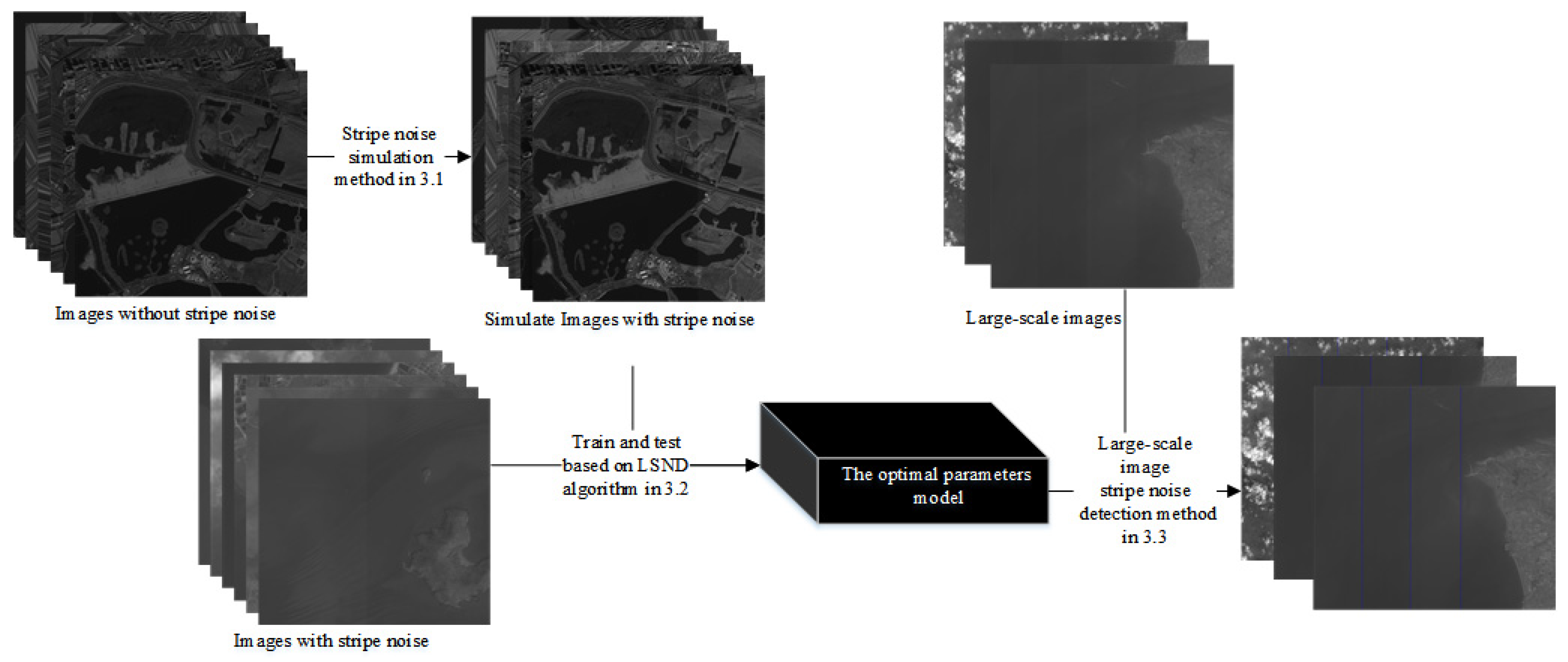
We used a linear neighborhood transformation on high-resolution remote sensing images to generate a large-scale stripe noise image dataset based on the stripe noise simulation method. Then, we used a new, deep neural network algorithm (LSND) for training based on the stripe noise image dataset to obtain a new detection model for the detection of stripe noise. A flowchart of this process is shown in Figure 2.

3.1. Stripe Noise Simulation Method

Considering push-broom imaging, the stripe noise in the image was mainly due to the following three reasons.
(1) The sensor is a linear response function within the spectral response range, and the relationship between the image gray value D and the received real radiance T can be expressed as
D = AT + B + ξ
Formula (1): A and B are the gain and offset of the sensor response function, respectively, and ξ is the noise. Owing to the differences in the responses of different sensors to the same incident light intensity from the outside, a grayscale output deviation was produced in the image, and stripe noise was generated [50].
(2) The stripe noise caused by the splicing of the charged-coupled device (CCD) linear array was mainly due to the manufacturing process of the CDD device and incomplete calibration before launch.
(3) The stripe noise was caused by random noise, electronic noise, or link noise.
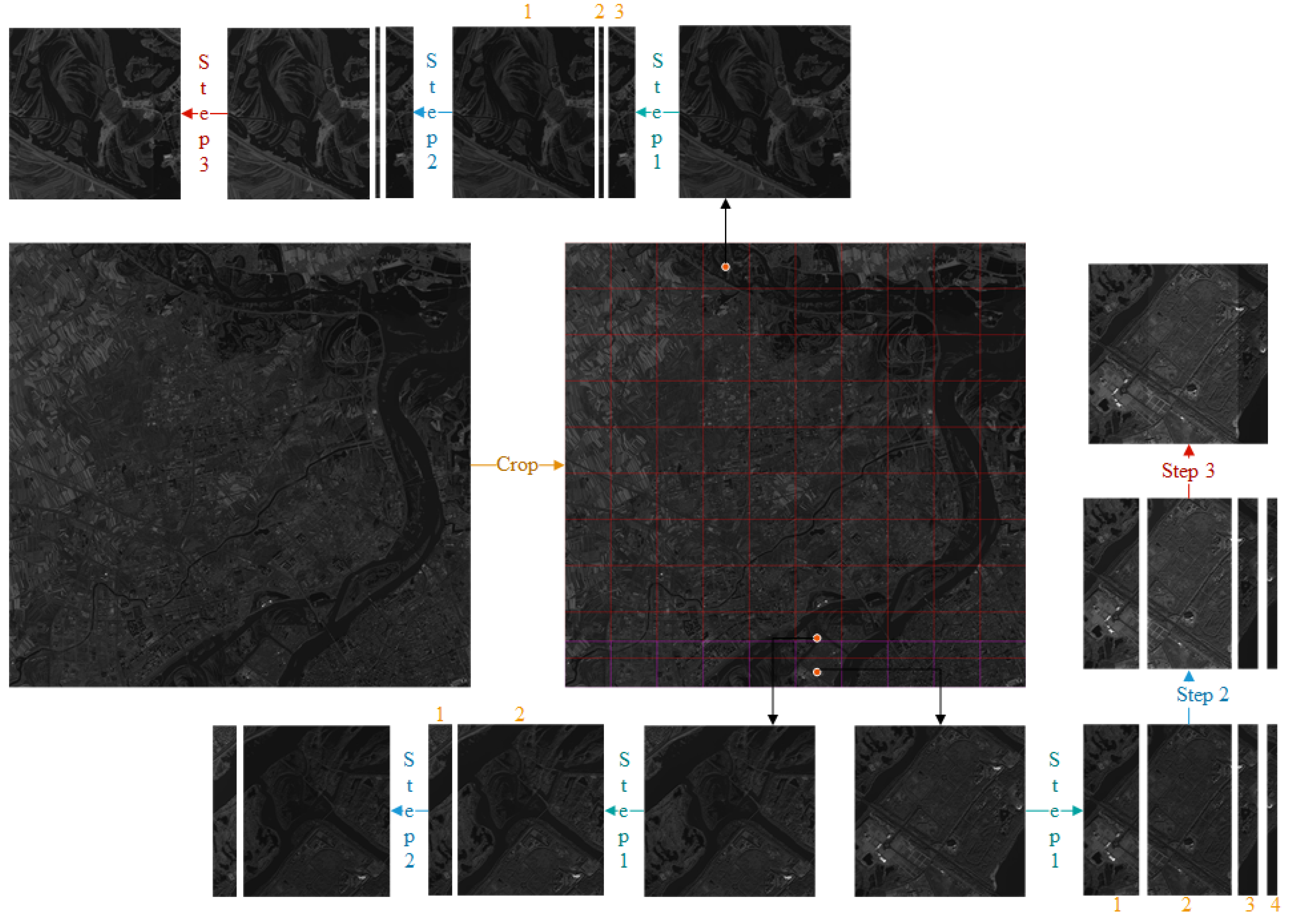
For a remote sensing image of a whole scene, we first divided the whole image, row-by-row and column-by-row, with KSIZE as the interval along the row and column direction (the value of KSIZE is 640 in this article), and obtained a lot of basic sample images of KSIZE × KSIZE size. Each row or each column that did not meet the width of KSIZE at the end, was cropped from right to left or bottom to top to obtain the basic sample images. Based on the causes of stripe noise and the transformation characteristics of the gray values, the simulation of stripe noise for each basic sample image consisted of the following steps, as shown in Figure 3:
(1) We randomly divided M small images in the row direction of the image (in this study, M was set in the range of 2 to 5), and numbered all small images (indicated by orange numbers in Figure 3).
(2) For M small images, along the cropping direction, we multiplied all the pixel values in the number 2 small image by the random numbers α and β. The value of α was [0.75, 1.25], and that of β was [−5, 5]. We adhered to the following: if M is 2, then end (as shown in the lower left corner of Figure 3); otherwise, proceed to step 3.
(3) We processed the next small image, regenerated the random numbers αnew and βnew, and kept the value range unchanged. If the absolute difference between αnew and the previous α was less than 0.2, we added 0.2 to the previous α to replace the αnew; otherwise we kept αnew. We multiplied all the pixel values in this small image by αnew/previous α and added a random number βnew, the calculated αnew/previous α and βnew, and reassgined α and β.
(4) We repeated step (3) until the end.
This simulation method is based on the characteristics of the linear response function. Compared with the excessive difference in the pixel values without the constraints by α and β, our method can improve robustness and diversity. Furthermore, it can also simulate random noise by adding random numbers.

3.2. Linear Object Detection Algorithm for Stripe Noise

The sizes of high-resolution remote sensing images, such as WorldView, IKONOS, DigitalGlobe, and GF-2 images, are quite large. Therefore, in addition to the accuracy, efficiency is an essential factor in the selection of the framework of the deep CNN. Combining the characteristics of stripe noise detailed in Section 3.1 and object detection algorithm described in Section 2.2, based on YOLOv4 [44]—which has excellent accuracy and speed—we developed a new network structure framework and designed a new loss function and non-maximum suppression method. Combining the above methods, we propose a new stripe noise detection algorithm called LSND.

3.2.1. Network Structure Framework

The YOLOv4 network structure framework is an extension of previous versions of YOLO and adds a large number of existing improvements. It is mainly composed of the CSPDarknet53 backbone network, SPP-Net, path aggregation, and YOLOHEAD. Compared with the previous YOLO, the backbone network has increased CSP structure and incorporates the Mish function. The backbone network not only ensures the accuracy of detection but also reduces the computational complexity of the algorithm. SPP-Net significantly increases the acceptance field, separates the most crucial context features, and does not reduce the network training speed. Path aggregation improves the detection of small objects through up-sampling, enhances the feature pyramid through down-sampling, and finally predicts detection through multi-scale feature layers.
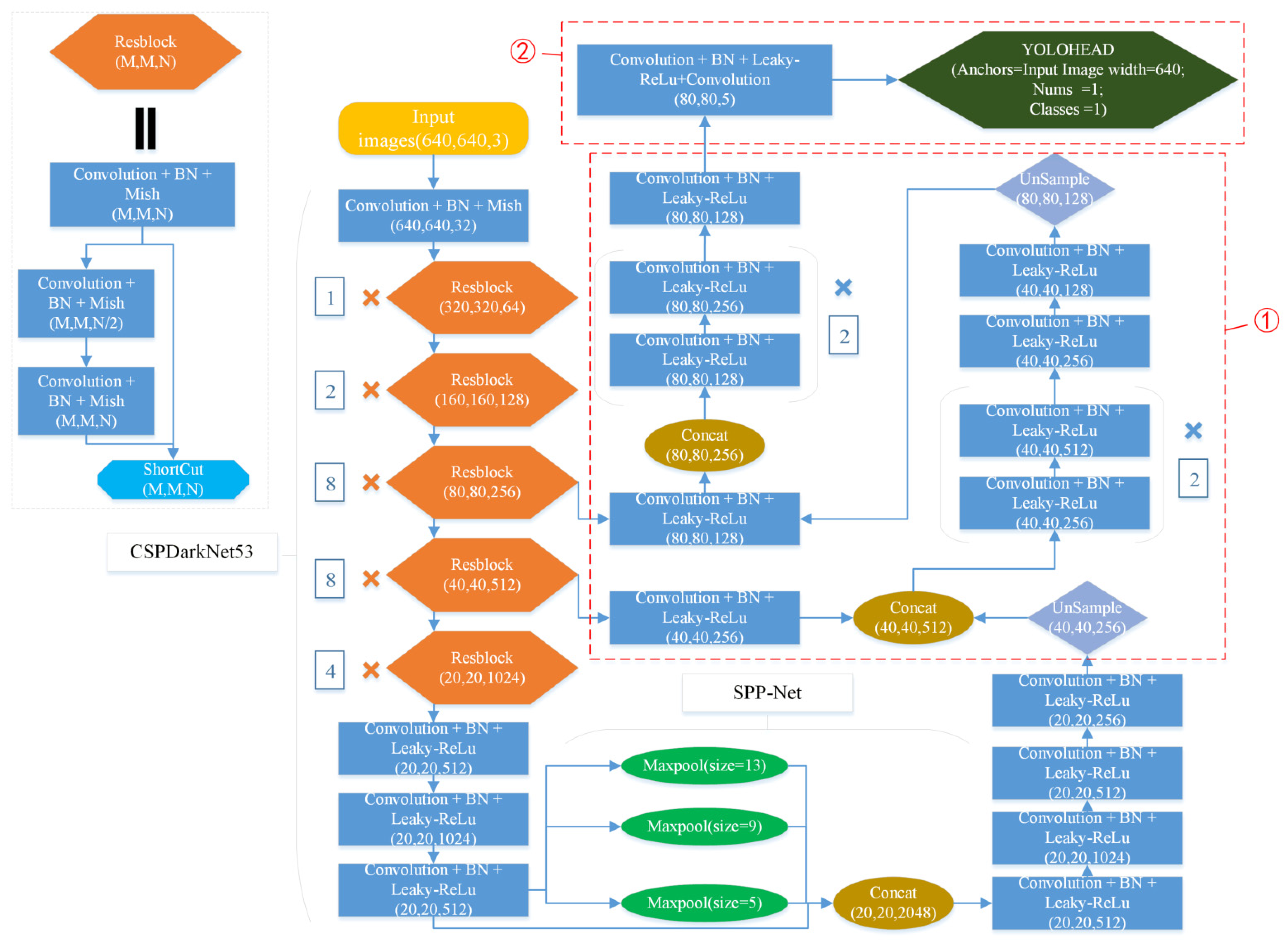
For the detection of single-class linear objects such as stripe noise, on the one hand, the stripe noise appears to penetrate the entire image from the top to bottom and the length of the detection object is consistent with the size of the image; on the other hand, the detection result is different from the previous two-dimensional bounding box and only contains the four basic parameters of the center point coordinates, that is, the length of the stripe noise and the confidence (x, y, h, confidence). Based on the YOLOv4 network structure framework, the LSND network structure framework for the detection of linear objects was designed, as shown in Figure 4.
The LSND network structure framework retains the CSPDarknet53 backbone network and SPP-Net. However, in the path aggregation part (as shown in Figure 4, part ①), the LSND network structure framework obtains large-scale features through up-sampling and proposes feature fusion, but discards the down-sampling part, retaining only one detection part. In the detection part (as shown in Figure 4, part ②), the detected image is divided into several grids to predict the center point coordinates and length of the detected object. For each grid, the width of the image is used as the prior length of the prediction line, and a prediction line is set. Considering the four basic parameters (x, y, h, confidence) and the parameter for predicting the line classification, the output dimension tensor is 1 × (4 + 1) = 5.
The structural framework design of the LSND network has the following considerations. First, compared with bounding box detection, the detection of linear objects requires a high degree of matching. When detecting objects in the bounding box, the error of one pixel from the real label is considered to be a negligible error, but when predicting linear objects, this situation is considered to be a detection failure. In previous network models combined with FPN [51], such as YOLOV4, owing to the large interval between the grid center points in the small feature map, when the center point of the predicted object is present in the grid, the accuracy of the parameters required to predict the center point of the linear object is high, making training difficult. The LSND network retains the detector part and only predicts a larger feature map. On the one hand, multi-scale prediction leads to a decrease in accuracy. In contrast, discarding multi-scale prediction reduces the overall parameters of the network and improves the training and detection speed of the model. Second, a single-class object detection method is used in this study, wherein the classification results of the prediction line are used as an auxiliary to determine the existence of detection objects. When detecting multi-class objects, the classification parameter is considered a separate variable.

3.2.2. Loss Function

For the YOLOv4 bounding box regression prediction, the results are completely unrestricted in the prediction range of the width and height, which can lead to gradient disappearance and instability. Moreover, when the center point parameter is zero, the predicted center point coordinates do not fall at the center of the prediction grids. Therefore, based on the premise of detecting linear objects, the LSND combines the bounding box regression prediction adopted by Scaled-YOLOv4 [52] to solve the above problems, as shown in Equations (2)–(4):
b x y = 2 δ ( t x y ) - 0.5 + C x y
b h = 4 δ ( t h ) 2 P h
δ ( x ) = 1 1 + e x
where txy represents the offset of the center point coordinates of the prediction line in the x- and y-axes; th represents the offset of the predicted line length of the model; Cxy represents the coordinates of the upper left corner of the grid where the center point of the actual line to be detected is located; Ph represents the prior length; and bxy and bh are the regression results.
The loss function of the LSND is composed of the confidence loss, classification loss, and position offset loss. The position offset and confidence losses are combined with the YOLOv3 [43] loss function and modified. The total loss function is given by (5).
L O S S = i = 0 s 2 I i o b j [ α 1 ( b x i b x i Λ ) 2 + α 2 ( b y i b y i Λ ) 2 + α 3 ( b h i b h i Λ ) 2 k ] i = 0 s 2 I i o b j [ C i Λ log ( C i ) + ( 1 C i Λ ) log ( 1 C i ) ] λ n o o b j i = 0 s 2 I i n o o b j [ C i Λ log ( C i ) + ( 1 C i Λ ) log ( 1 C i ) ] i = 0 s 2 I i o b j c c l a s s e s [ P Λ i log ( p i ) + ( 1 p i Λ ) log ( 1 p i ) ]
The first term represents the position offset loss, the second and third terms represent the confidence loss, and the fourth term is the classification loss.
Equation (5) indicates that the feature map is divided into S × S grids. Each grid generates one anchor line, which corresponds to the prediction line obtained by the network. If a real detection object center point is present in the grid, only the confidence loss is calculated; otherwise, the position offset loss must be calculated. The confidence loss adopts a cross-entropy loss function, which is divided into two types: detection objects and non-detection objects. In non-detection objects, adding the weight coefficient λnoobj to the loss without detection objects can reduce the contribution weight of the loss value without the object to the total loss. The position offset loss is obtained by modifying the mean squared error loss function, where α1, α2, α3, and k are used to balance the weight coefficients bx, by, and bh (in this study, the ratio of α1, α2, and α3 was 4.0, 1.0, 0.4, respectively, and k was the ratio of input and output image size). The classification loss uses a cross-entropy loss function; when the predicted object in the grid corresponds to a real object, it calculates the classification loss.

3.2.3. Non-Maximum Suppression of Linear Objects

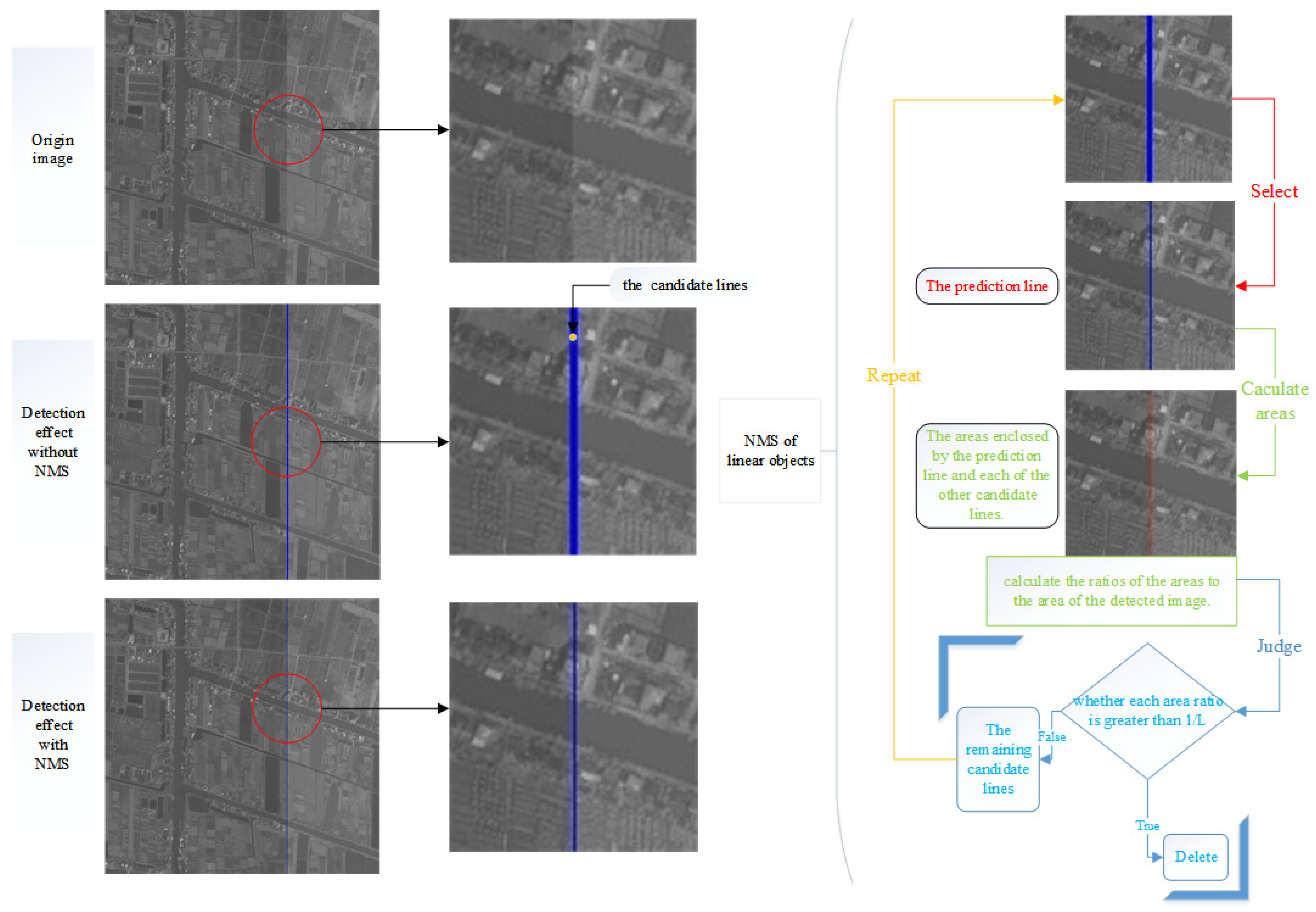
In detection tasks, NMS (non-maximum suppression) is often the last step, which is a post-processing algorithm for performing redundancy removal operations on the detection results. Previously, IoU, DIoU, and CIoU have been used as indicators of judgment thresholds in detection tasks. The value of the intersection area between the prediction box and the real box divided by the union area, that is, IoU (intersection over union) is used as the basis for judging whether the prediction box is true. DIoU and CIoU [53] are enhanced versions of IoU. In addition to considering the overlap area, DIoU adds the distance between the center points; CIoU adds the aspect ratio on the basis of DIoU. However, in this study, the above indicators could not be used as judgment thresholds for the detection of linear objects. We improved the non-maximum suppression to detect linear objects. The operation steps are as follows, and shown in Figure 5:
(1) We sorted the candidate lines generated in the image in descending order of confidence, and subsequently deleted the candidate lines whose confidence was less than the minimum confidence value (in this study, this was set to 0.3). We finally selected the candidate line with the highest confidence as the prediction line.
(2) We calculated the ratios of the areas enclosed by the prediction line and each of the other candidate lines to the area of the detected image.
(3) We judged whether each area ratio was greater than the threshold value (in this study, the value was 1/L, where L was the width of the detected image); we abided by the following: if true, delete it.
(4) For the number of remaining candidate lines, if there was only one, we considered it as a prediction line, then end; otherwise we repeated the above steps for all the remaining candidate lines.

3.3. Large-Scale Image Stripe Noise Detection Method

For a large size of the original high-resolution satellite imagery, it is difficult to directly use data from a truly whole image for training. Based on the characteristic that the stripe noise runs through the entire image, a cropped image is randomly selected from each column as the detection representative of each column during the detection process. On the one hand, the use of local information instead of the overall information can reduce the amount of computation and improve detection speed; on the other hand, good detection results based on different positions also reflect the superiority of model detection from the side. Furthermore, we chose to detect from different starting positions in order to overcome the problem of not being able to detect stripe noise in the clipping. After using different starting positions, it can be detected more comprehensively and holistically. Therefore, we used the following steps for whole image detection, as also shown in Figure 6:
(1) For the two different row coordinates of the starting positions, when the row coordinate of starting position was 0, we used the above method in Section 3.1 to crop a truly entire image to obtain the cropped real images; otherwise, we also started from the starting position to crop, row-by-row and column-by-column, to obtain the cropped real images; however, when the rest area was not satisfied with the crop size, we did not select it. Then, we recorded the relative positions of the cropped real images on the entire image, and randomly selected a cropped image for each column on the entire image.
(2) The cropped images randomly selected from each column were detected using the optimal-parameter model based on the LSND algorithm, and we recorded the detection results.
(3) The row coordinate of the detection results of each column, plus the row coordinate of the starting position (as shown in the lower right corner of Figure 6: the cropped image detection result based on the second starting position (0--319.99--319.95--640.00--0.99 (category--center point x--center point y--Length--Confidence)) transformed to (0--639.99--319.95--640.00--0.99), and were put together. The results were filtered using the non-maximum suppression of linear objects method in Section 3.2.2 for the filtered detection results.
(4) For the filtered detection results, we concatenated them along the row direction and transformed the length into the image column direction length to obtain the strip noise detection effect for a whole remote sensing image.

4. Experiment and Analysis

Based on the LSND algorithm, simulated images with stripe noise were input into the algorithm for training and evaluation. The operating system was Ubuntu 18.04 LTS, the graphics card model was NVIDIA Quadro M4000, and the video memory was 16 GB. The Visual Studio Code, python 3.7.4, pytorch 1.7.1, cuda 10.1, and cudnn 7.3.1 software packages were used.

4.1. Dataset

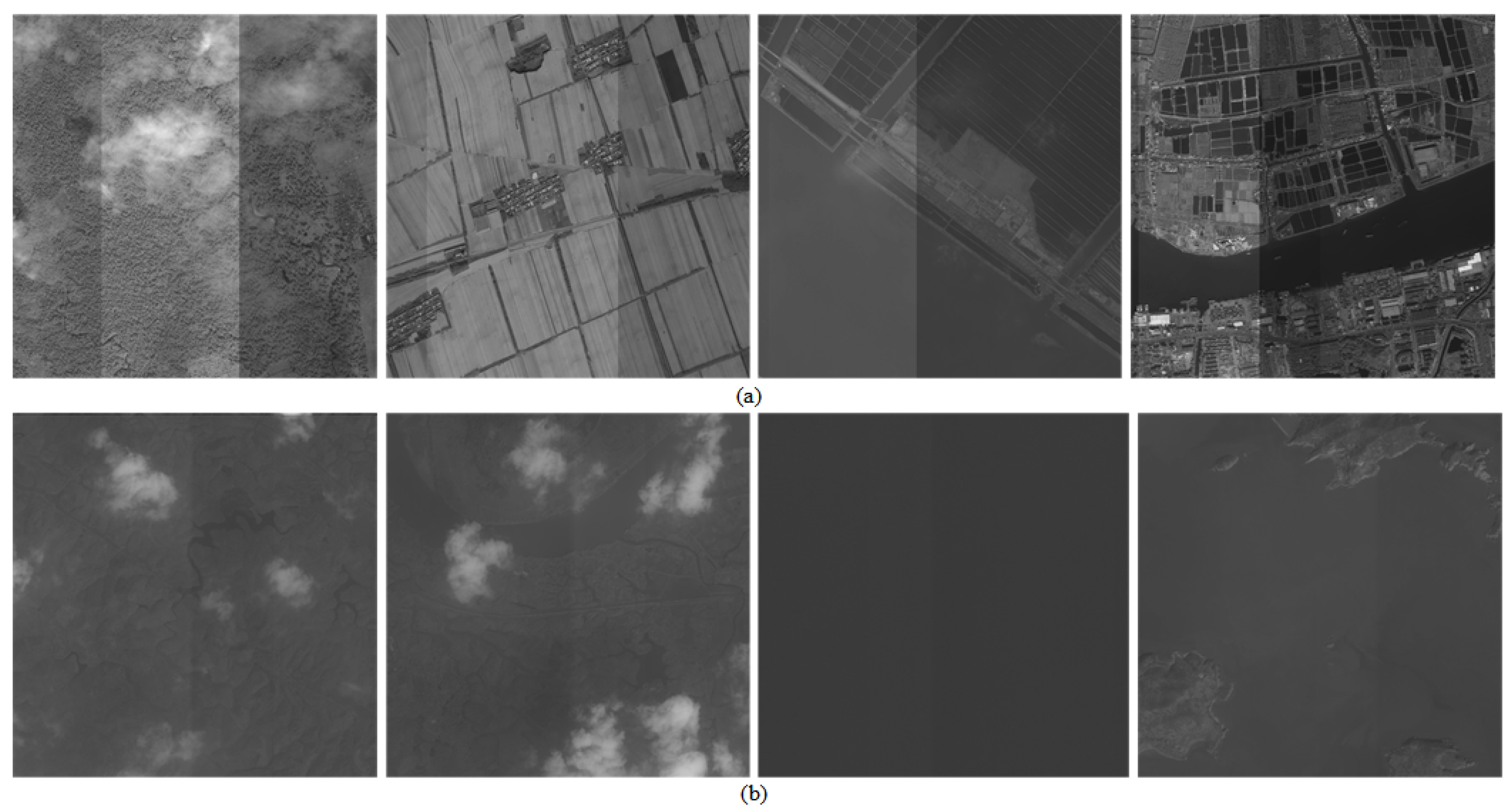
First, owing to the massive volume of image data in the TIFF format, the images were converted to the JPG format to reduce the data volume. Then, along with the row and column directions at 640 intervals, the transformed images were segmented row-by-row and column-by-column, and many 640 × 640 sized basic sample images were obtained. Finally, the basic sample images were simulated using the stripe noise simulation method detailed in Section 2.1, and the remote sensing images with stripe noise were obtained. The comparison between the simulated and real images with stripe noise is shown in Figure 7. It can be seen from the figure that the simulated data and the real data have similar properties in terms of morphological characteristics, texture characteristics, and contrast. Moreover, the simulated strip noise can appear on rich ground objects such as farmland, ports, etc., and the sample diversity can be greatly supplemented. This is more conducive to improving the robustness of the model.
In the simulation process, the center point coordinate and length information of the stripe noise of each image were saved and converted into the corresponding labels sequentially. In addition, for comparison with previous deep learning detection algorithms, we added the width W (equal to 2 in this study) to each stripe noise label to generate a label in the form of a bounding box. In this paper, the two types of labels are defined as line and box labels, as presented in Table 2 and Table 3.
Finally, all stripe noise images and labels obtained with the simulation were divided into training and validation sets in the ratio of 14:1. The number of images in the training set was 178,070, and the number of images in the validation set was 12,500.

4.2. Training

To test the LSND, similar algorithms were selected for training and compared. First, when detecting linear objects, there is a large interval between the grid center points divided on the small feature map, as detailed in Section 3.2.1, which makes training challenging. Therefore, the addition of small feature maps for prediction may decrease the detection accuracy. To verify the accuracy of our design, the backbone network, SPP-Net, and path aggregation of the YOLOv4 model were unchanged, and only the detector part of the YOLOv4 model was modified (i.e., the YOLOHEAD part) to obtain the new model. Each model detector of the new model, loss function, and other processing parts were the same as those of the LSND. In this study, the second new algorithm was named LS-YOLOv4 (an improved YOLOV4 for linear stripes). Next, we selected YOLOv4, and in the mainstream algorithms of the anchor-based and anchor-free models; we selected models with good performance in speed and accuracy, namely the RetinaNet and FCOS models. Finally, the selected LS-YOLOv4, YOLOv4, RetinaNet, and FCOS models were trained.
Based on the line labels, the generated dataset was inputted to LSND and LS-YOLOv4 for training and the exponential moving average (EMA) method was used to average the model parameters, to improve the test indicators and robustness of the model. The batch size was four, the number of training epochs was 50, and the initial learning rate was 0.001. The learning rate reduction technique employed the cosine annealing strategy [54]; the loss function optimization method was Adam [55]; the Adam parameters β 1 and β 2 were initialized to 0.937 and 0.999, respectively; and the weight-decay value of Adam was 0.005. The model parameters were updated after 16 batches. In the first three rounds of training, warm-up [56] was applied to the learning rate and β 1 parameter in the Adam function. In the first three rounds of training, the learning rate of each round decreased linearly from 0.1 to the learning rate obtained using the cosine annealing strategy during initialization, and β 1 increased linearly from 0.9 to 0.937. During the remainder of the training, the learning rate decayed according to the cosine annealing strategy, and β 1 in Adam remained unchanged at 0.937 until the training ended.
Based on the box labels, we trained YOLOv4, RetinaNet, and FCOS using the dataset. The loss function was the same as that used in the original work. The initialization values, such as the batch size, number of training rounds, and learning rate settings, remained unchanged. The confidence threshold and IoU threshold were the default values of the algorithms in the original works until training ended.

4.3. Loss Curve Analysis

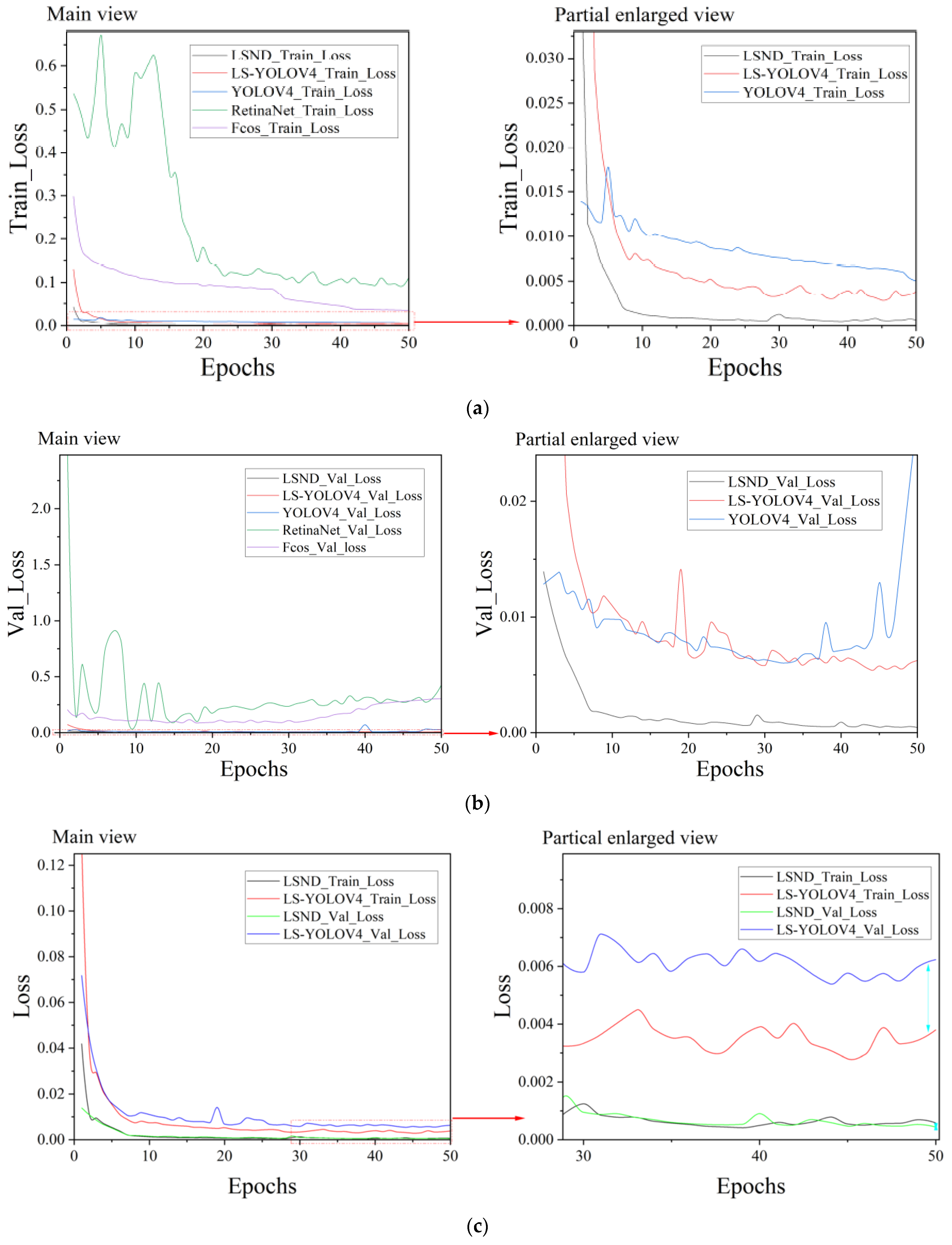
Based on the LSND, LS-YOLOv4, YOLOv4, RetinaNet, and FCOS, 50 epochs of training were performed, and the loss curves of the training and validation sets were obtained. The loss curves (LSND and LS-YOLOv4) on/for the training and validation sets are compared in Figure 8.
Analyzing the figures, it can be seen that, on the one hand, the LSND loss curve converged faster on both the training and validation sets compared with the other loss curves, with a smaller convergence loss compared with the others. In contrast, analyzing the loss curves of the LSND and LS-YOLOv4 for the training and validation sets, the LSND achieved better results in terms of both deviation and variance. This demonstrates that the LSND is more suitable for the detection of linear objects than LS-YOLOv4.

4.4. Model Evaluation

The new model incorporating LSND was evaluated and compared based on the determined model-evaluation index and prediction confidence threshold. Concurrently, to test the robustness and versatility of the model, input images of different sizes were selected to compare the LSND and LS-YOLOv4 based models.

4.4.1. Model Evaluation Indicators

Precision, recall, AP, and F1-score are fundamental concepts and indicators in object detection. The calculation of these parameters is shown in (6)–(9):
P r e c i s i o n = T P ( T P + F P )
R e c a l l = T P ( T P + F N )
A P = 1 C K = i N P ( k ) Δ r ( k )
F 1 S c o r e = 2 P r e c i s i o n × R e c a l l P r e c i s i o n + R e c a l l
where TP represents the number of correctly identified stripe noises; FP is the number of backgrounds misrecognized as stripe noise; FN represents the number of unrecognized stripe noises; N represents the number of all stripe noises to be detected; P(k) represents the value of precision when k stripe noises are recognized; and Δ r ( k ) represents the change in the recall value when the number of recognized stripe noises changes from k − 1 to k (by adjusting the threshold).

4.4.2. Determination of the Prediction Confidence Threshold

This study focuses on linear object detection. The IoU, DIoU, and CIoU cannot be used as indicators to assess the confidence threshold of the prediction. On the one hand, a linear object has one-dimensional characteristics. On the other hand, it ensures the accuracy of the judgment between the predicted and the actual results. The threshold was set as detailed below.
For an M × M image, the threshold was set to M 1 M when the ratio of the area enclosed by the predicted and actual lines to the total area of the image was less than 1 M . In this case, the stripe noise was considered to be correctly identified.
In addition, ten values were obtained at equal intervals in the interval [ M 1 M , 10 × M 1 10 × M ] as the threshold value of the judgment sample used in the AP calculation.

4.4.3. Analysis of the Evaluation Indicators

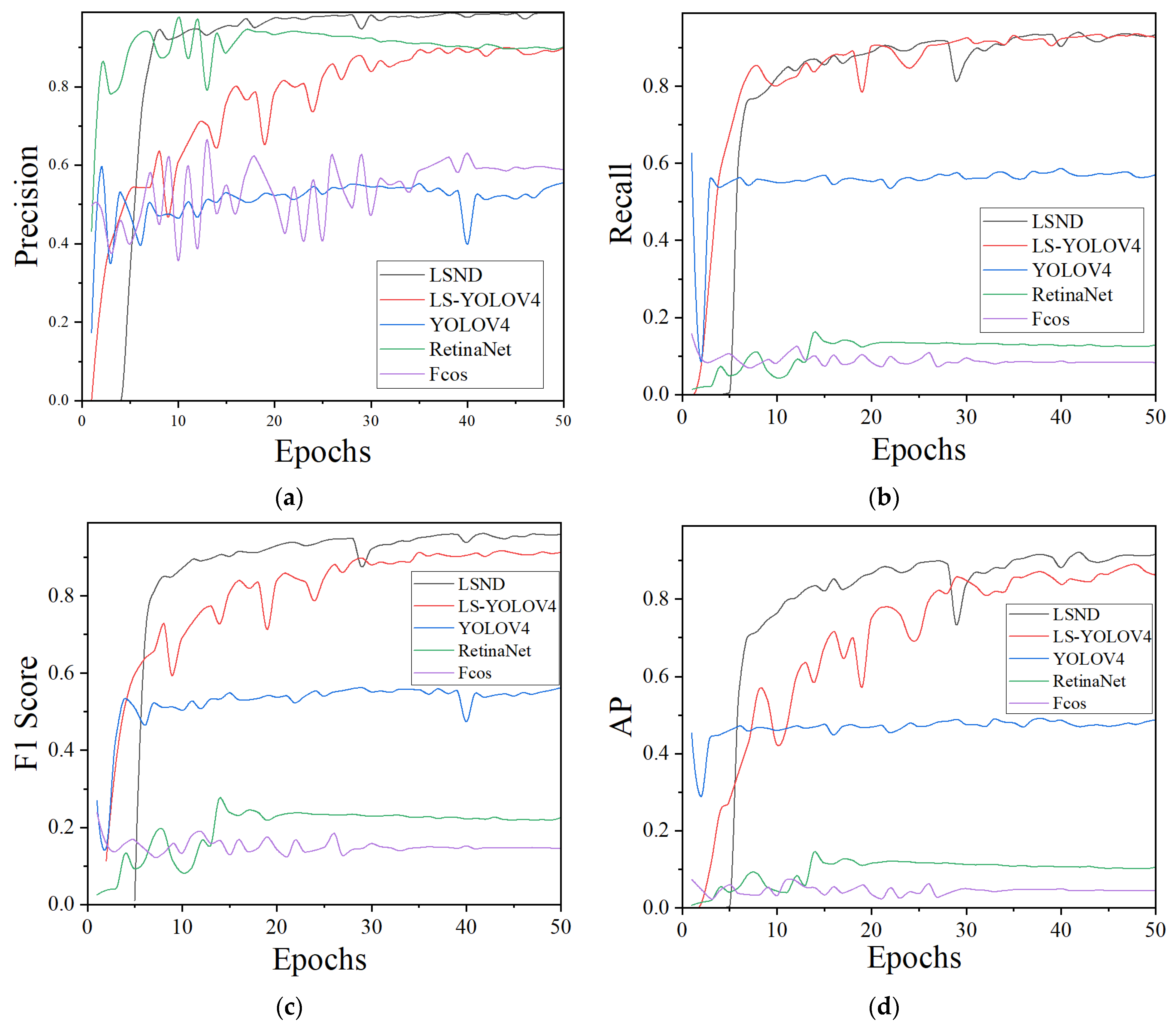
In Section 4.1, the box labels based on the line labels were obtained by increasing the width (equal to 2 in this study), which means that each box label was generated by adding a one-pixel width to both the left and right sides of each line label. In the case of YOLOv4, RetinaNet, and FCOS, the centerline of the prediction box was selected as the prediction line with the stripe noise in the image. Based on the evaluation indicators defined in Section 4.4.1 and Section 4.4.2, the models were evaluated on the validation set, as shown in Figure 9 and Table 4.
The table and figures show that the model-evaluation index curve obtained using the LSND converges very quickly. After convergence, the volatility of each evaluation index is small, and good performance is observed for each evaluation index, with a precision of 98.7%, recall of up to 93.8%, F1-score of 96.1%, and AP of 92.1%. The detection effect was better than that of the models using other algorithms.

4.4.4. Robustness Analysis

Based on the analysis presented in Section 4.4.3, it can be seen that the detection performance of the models based on the LSND and LS-YOLOv4 show promising results in terms of the different evaluation indicators. To test whether the two algorithms performed well on small-sized images, based on the stripe noise simulation method presented in Section 3.1, we created a small-sized (64 × 64 in this study) simulated noise image dataset. Furthermore, to ensure that the training time was similar to that of the 640 × 640 large-sized image dataset, the number of images in the training set was 250,280, and that in the validation set was 17,900. When training on small-sized images, the batch size was 512, and the remaining parameters remained unchanged.
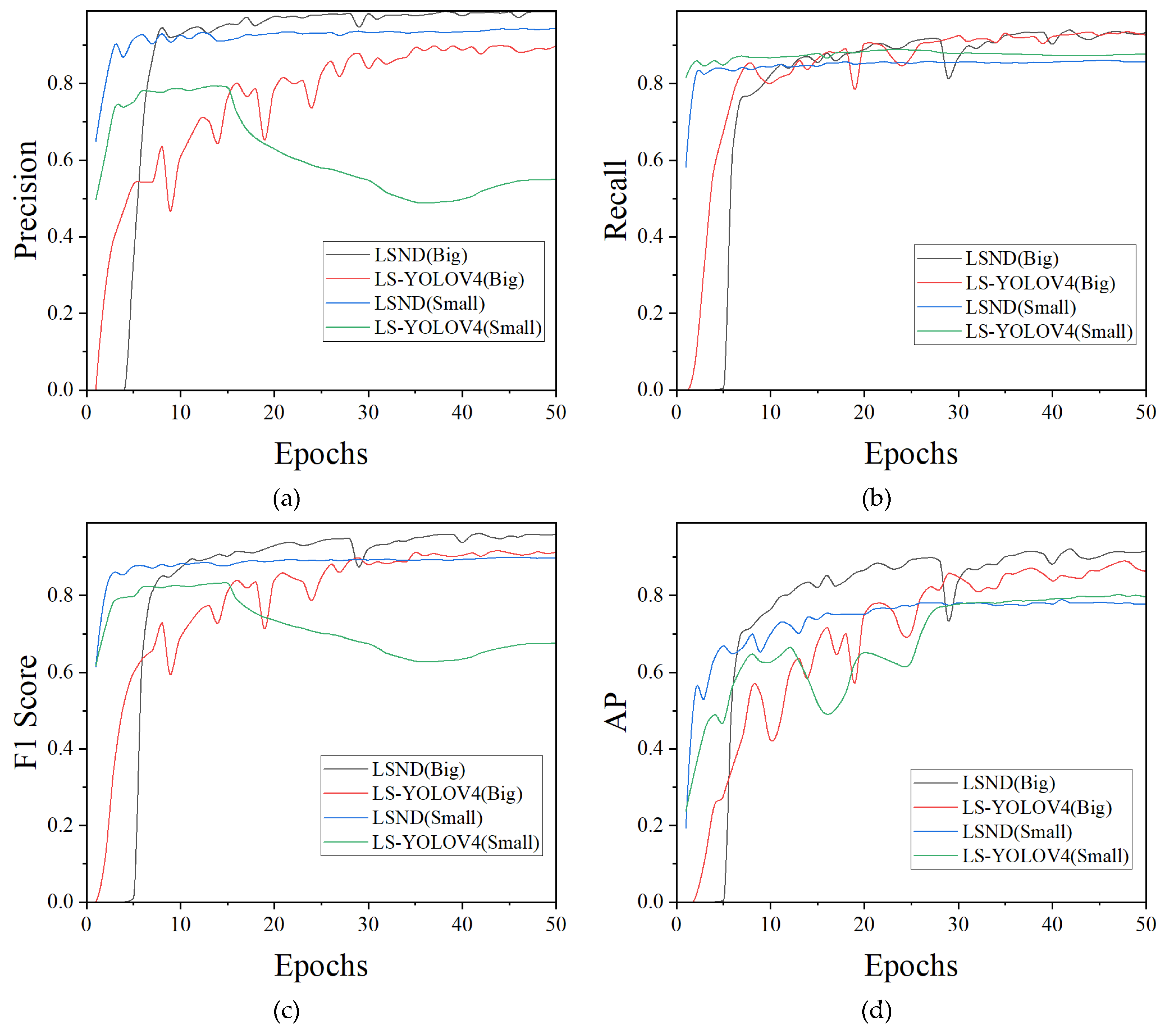
The small-sized dataset was trained using LSND and LS-YOLOv4, and the precision, recall, F1 value, and the AP values were recorded for the validation set after each round of training and plotted. We compared the evaluation index curves obtained after each round of training on small-sized images and large-sized images, as shown in Figure 10 and Table 5.
It can be seen from the various evaluation indicators that the model using LSND could quickly achieve high accuracy at different scales within a small fluctuation range; for small-sized images, the model using LSND performed better in terms of the precision and F1-score, with a precision of up to 94.3% and F1-score of up to 89.8%. By reducing the number of image features, the model using the LSND is more robust. The model detection accuracy was high, the fluctuation range was small, and the convergence speed was faster than the other models.

4.5. Image Detection Results

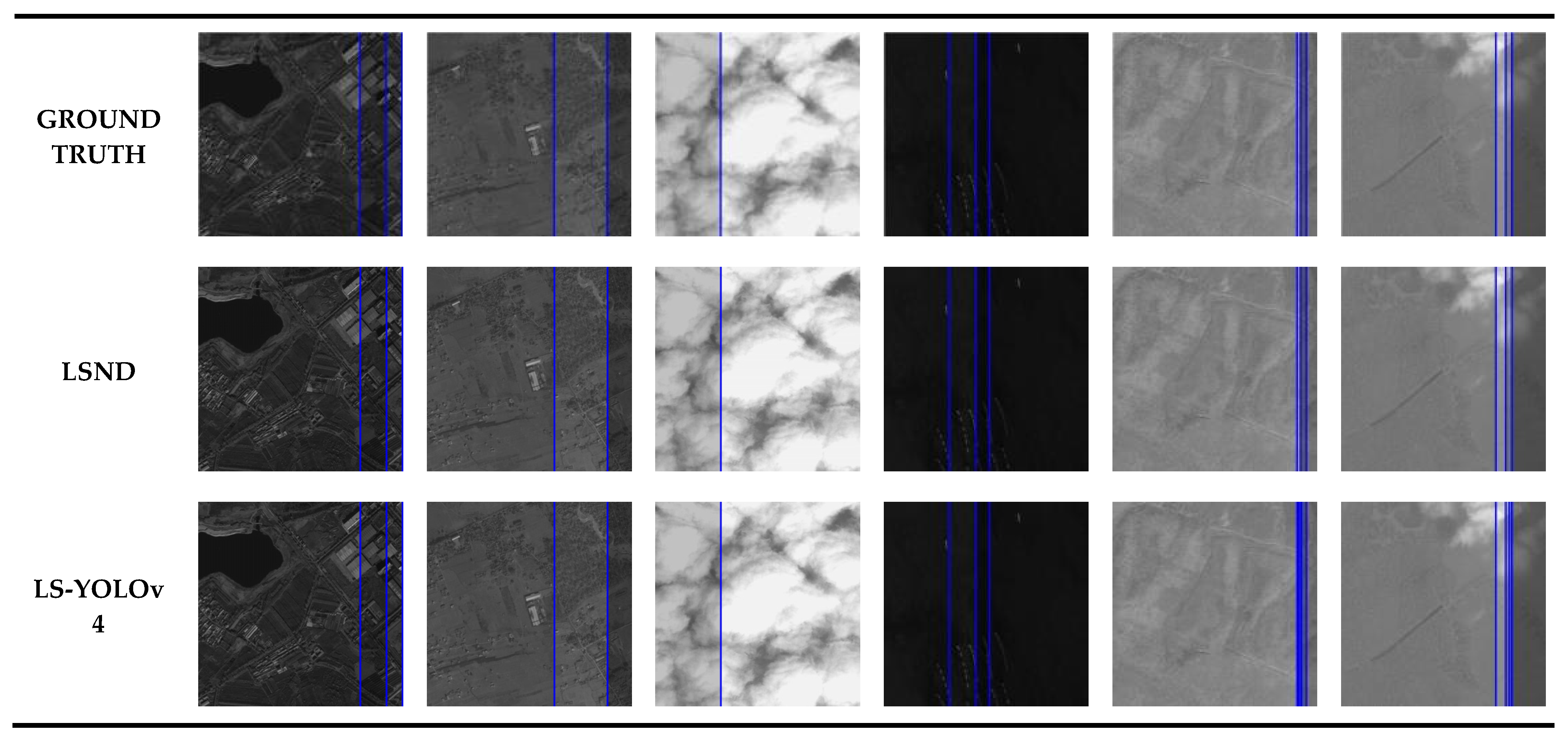
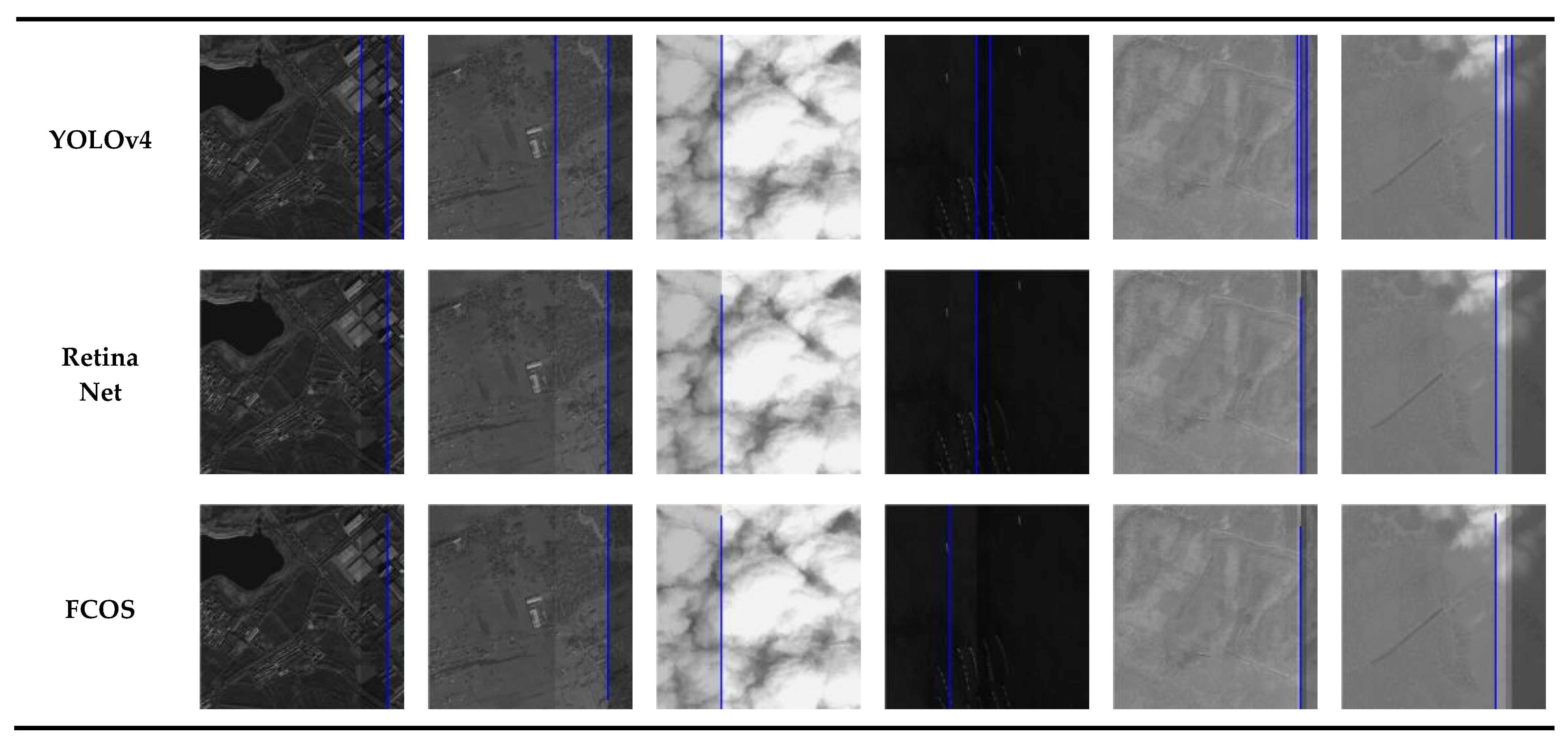
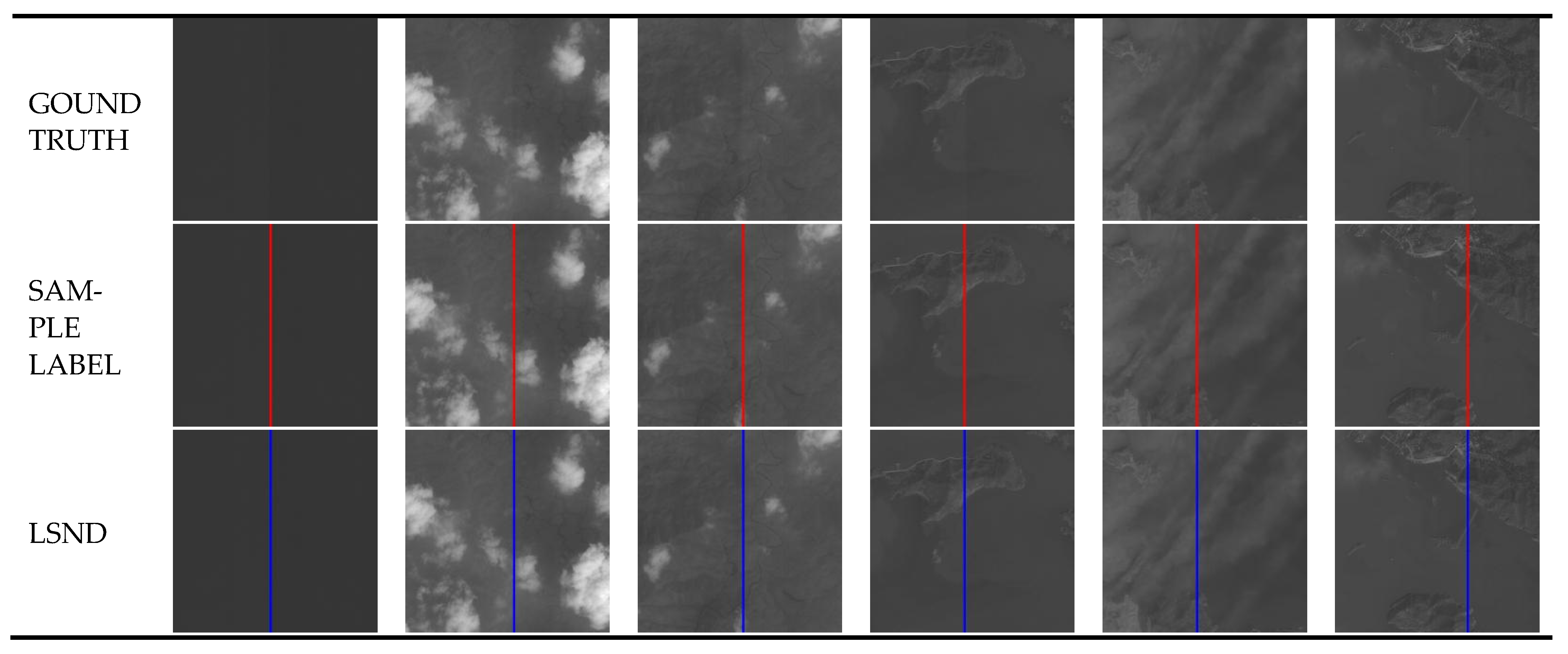
High-resolution remote sensing images with stripe noise were cropped to 640 × 640 sized images. In addition, to improve the detection efficiency, the cropped images were converted to a JPG format, and the stripe noise in the images was detected using five trained models based on LSND, LS-YOLOv4, YOLOv4, RetinaNet, and FCOS, as shown in Figure 11.
Figure 11 shows that for a variety of complex features such as mountains, clouds, and towns, the locations of the stripe noises are very close, and the shapes of the ground features are similar to that of stripe noise, which can lead to errors in the detection. The model using LSND achieved good performance in detecting complex stripe noises.
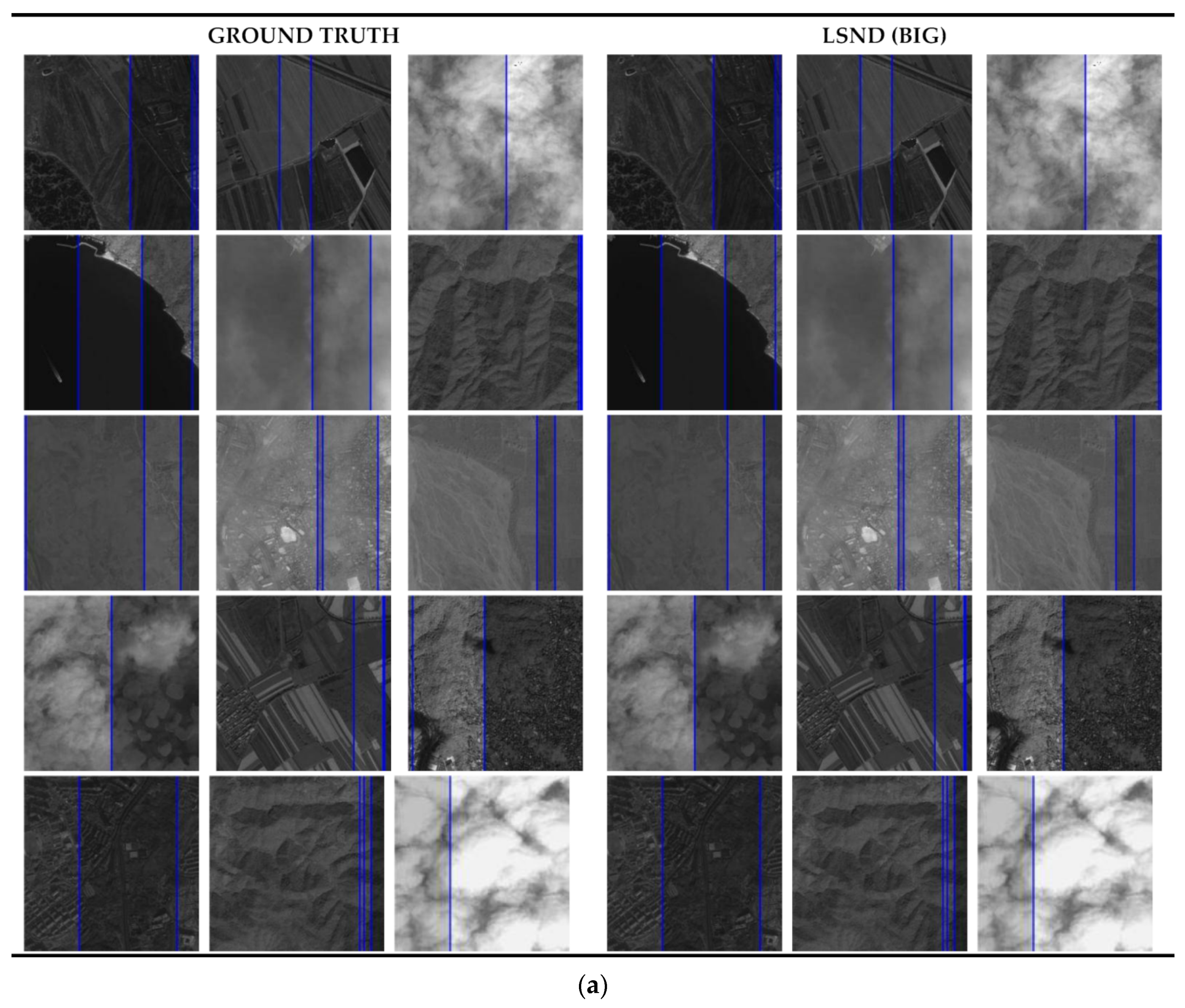
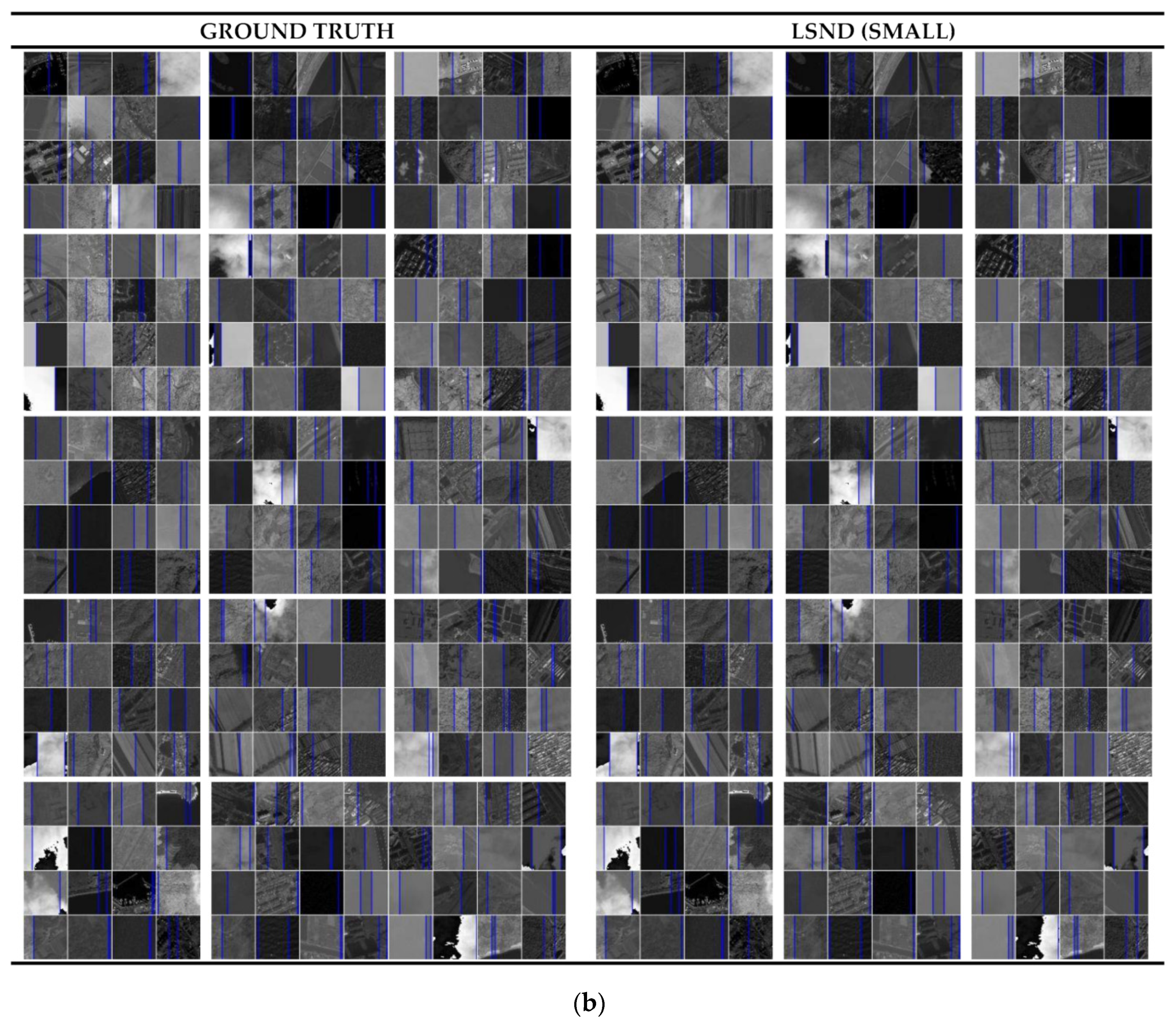
We visually verified the robustness of the LSND-based model. According to the above-described method, 64 × 64 and 640 × 640 sized images with stripe noise were obtained. The detection performance for LSND is shown in Figure 12. It can be seen that good detection performance was achieved on images of different scales, and in the case of large-scale images, an FPS of up to 35.71 was recorded, indicating a fast detection speed.

4.6. Real Image Detection Results

Firstly, we selected a small number of real data images containing stripe noise, and for each whole real remote-sensing data point, we divided the whole image, row-by-row and column-by-row and column, with KSIZE as the interval (the value of KSIZE in this paper is 640), and obtained a large number of the KSIZE × KSIZE size of the cropped real images. Then, for each row or column that did not meet the KSIZE width at the end, the basic sample images were obtained by cropping from right to left, or from bottom to top. Finally, based on the LSND algorithm, we trained the acquired cropped real images and the simulated images to obtain a new optimal-parameter model based on the LSND algorithm, the stripe noise in real images was detected using the new optimal-parameter model, as shown in Figure 13.
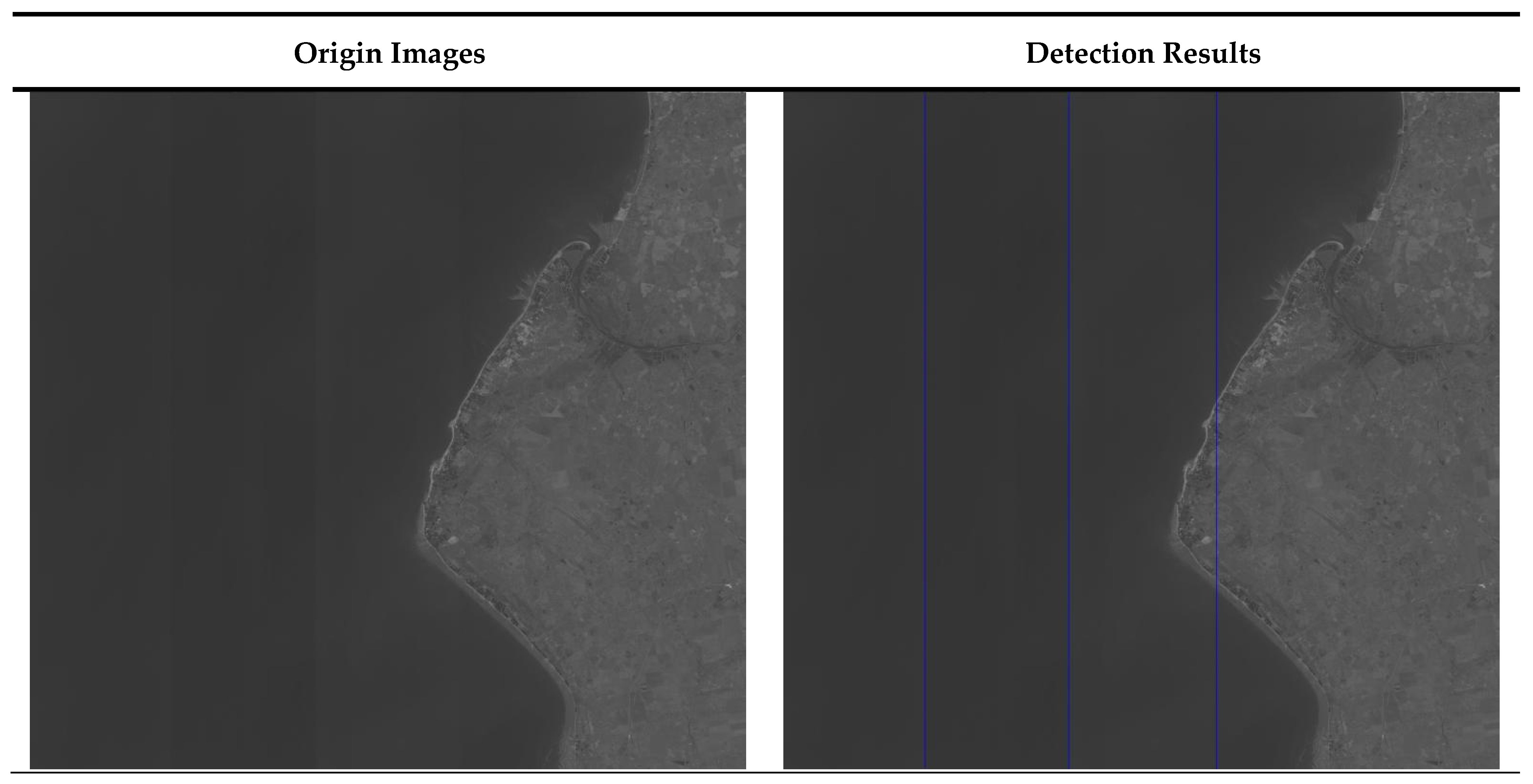
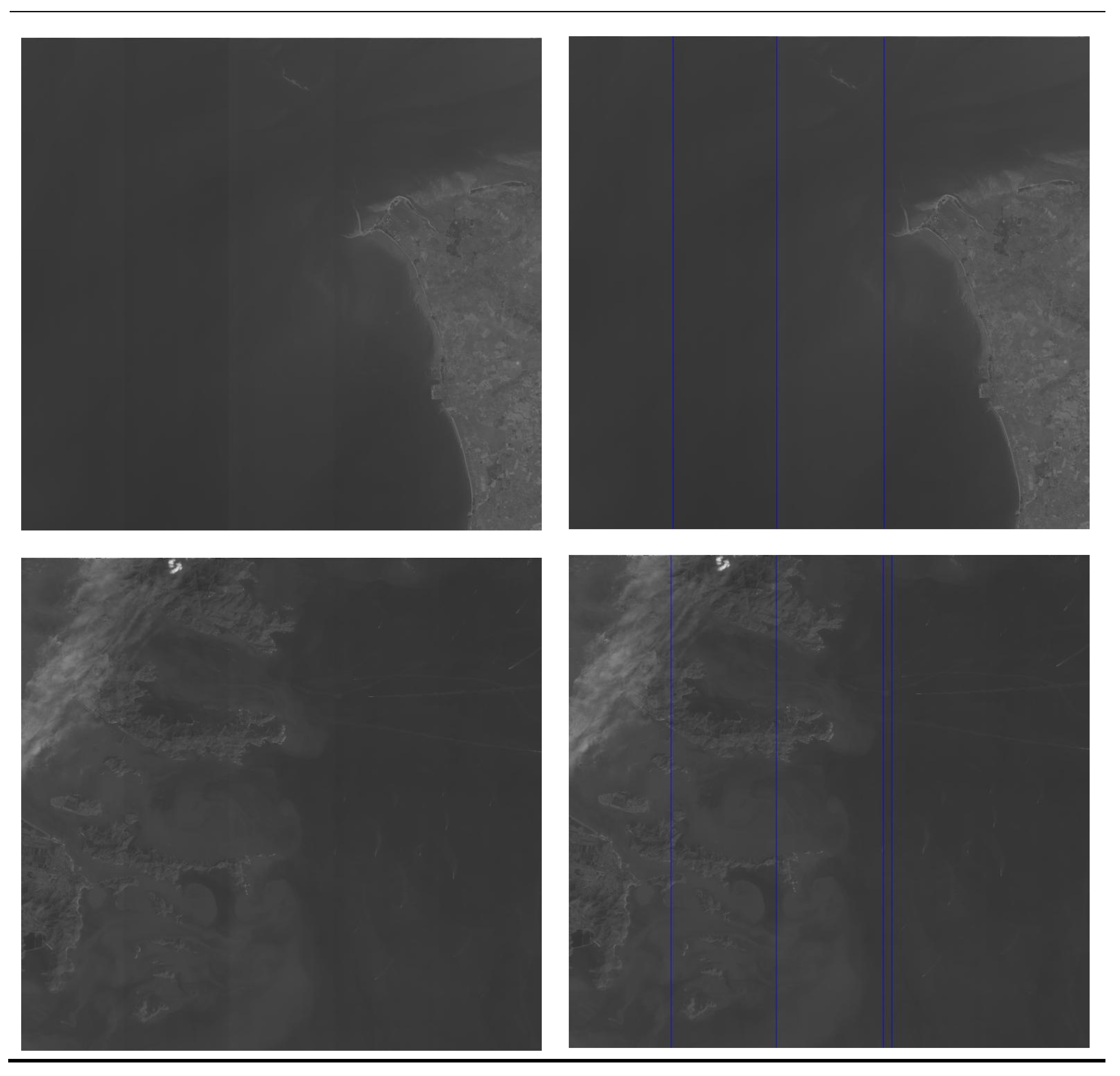
For a large size of the original high-resolution satellite images, based on the new optimal-parameter detection model, we used the large-scale image stripe noise detection method in Section 3.3 to detect the entire images. As shown in Figure 14, it can be seen that this performed well in terms of effect and accuracy.

5. Conclusions

In this study, we proposed an LSND-based model for detecting stripe noise in high-resolution remote sensing images. We simulated a large number of remote sensing images with stripe noise through linear transformation to generate the dataset. Then, we improved the path aggregation and classifier parts of the YOLOv4 network structure framework to obtain a new network structure framework, designed a new loss function for the training process and the non-maximum suppression of linear objects used in the detection process, and proposed a new linear stripe noise detection algorithm called LSND. The experimental results showed that the new detection algorithm achieved promising performance in terms of the different detection indicators in detecting objects of different sizes, with excellent speed.
Moreover, we trained the real images and simulated images to obtain a new optimal-parameter model based on the LSND algorithm; the stripe noise in real images was detected using the new optimal-parameter model, and the detection results were quite promising. In order to meet actual industrial needs, we adopted a series of processes to detect an entire image, and achieved very good results in terms of accuracy and time.
The proposed detection method can effectively detect the stripe noise of massive remote sensing datasets, and can use the detection results to evaluate the quality of the image, then adopt more targeted image processing methods to obtain high-quality images. Furthermore, these high-quality images, after processing, are further used in resource surveys, surface environmental monitoring, human activity monitoring, and many other capacities. However, some issues must be addressed in future studies. Firstly, improvements to the backbone network and transformer mechanism of the model [57] should be explored for the improved detection of stripe noise. Secondly, for the image data after image correction, the stripe noise has a certain inclination angle. Effective detection of oblique stripe noise is also considered for our future research.

Author Contributions

Conceptualization, B.L. and D.X.; methodology, Y.Z.; software, B.L.; validation, D.X., Y.W. and J.Y.; formal analysis, S.J.; investigation, B.L.; resources, L.Z.; data curation, Y.Z.; writing—original draft preparation, B.L.; writing—review and editing, B.L.; visualization, B.L.; supervision, D.X.; project administration, D.X.; funding acquisition, D.X. All authors have read and agreed to the published version of the manuscript.

Funding

This research was funded by [the National Key Research and Development Program of China] grant number [2018YFC0706003], [National Natural Science Foundation of China] grant number [42071318], [the National Key Research and Development Program of China] grant number [2017YFC0212302], [the program of Youth Innovation Promotion Association of CAS] grant number [Y93020033D]. And The APC was funded by [2018YFC0706003].

Institutional Review Board Statement

Not applicable.

Informed Consent Statement

Not applicable.

Data Availability Statement

Code used in this study can be made available by the authors upon request.

Conflicts of Interest

The authors declare no conflict of interest.

Appendix A

Table A1. Model characteristics, public test accuracy, and innovation points of the main object detection algorithms. In this table, if the test dataset is from the VOC2007, mAP/%@IoU = 0.5; if the test dataset is from the MSCOCO, mAP/%@IoU = 0.5:0.05:0.95.
AlgorithmsBackbone Input Size/PixelTest DatasetmAP/%Speed f/sInnovation Points
R-CNN [33]TWO
STAGE
MODELS
VGG161000 × 600VOC
2007
58.50.5Uses a large number of CNNs to apply bottom-up candidate regions to locate and segment objects.
SPP-Net [34]ZF-51000 × 600VOC
2007
59.22Uses the spatial pyramid pooling structure.
Fast R-CNN [35]VGG161000 × 600VOC
2007
703Based on the R-CNN, an improved ROI pooling layer is used. The feature maps of differently sized candidate frames are resampled into fixed-size features.
Faster R-CNN [36]VGG161000 × 600VOC
2007
73.27Based on Fast R-CNN, it proposes the use of a region proposal network (RPN) to generate candidate regions and integrate the steps of generating the candidate regions, feature extraction, object classification, and position regression into a model.
R-FCN [37]ResNet-1011000 × 600VOC
2007
80.59Solves the contradiction between “translation-invariance in image classification” and “translation-variance in object detection”, and uses “Position-sensitive score maps” to improve detection speed while improving accuracy
Mask-RCNN [38]ResNeXt-1011300 × 800MS
COCO
39.811Based on Faster R-CNN, it proposes the replacement of the ROI pooling layer with ROI Align, and uses bilinear interpolation to fill the pixels at non-integer positions. No position error occurs when the downstream feature map is mapped to the upstream.
Cascade RCNN [39]ResNeXt-101-FPN1300 × 800MS
COCO
42.88It is composed of a series of cascades of detectors with increasing IoU thresholds. With increasing thresholds, high-quality detectors can be trained without reducing the number of samples.
SSD [40]ONE
STAGE
MODELS
VGG16300 × 300VOC
2007
7.146Based on the feature map output by different convolutional layers, it detects objects of different sizes.
YOLOv2 [41]DarkNet-19544 × 544VOC
2007
8.640(1) Increases the number of candidate boxes compared with the YOLO and uses a powerful constraint positioning method. (2) Proposes multi-scale feature fusion. (3) Use the K-means clustering method for clustering to obtain the anchor boxes.
RetinaNet [42]ResNet-101-FPN800 × 800MSCOCO39.15Uses the focal loss function to solve unbalanced sample numbers in different categories.
YOLOv3 [43]DarkNet-53608 × 608MS
COCO
3320(1) Based on YOLOv2, it changes the backbone. (2) The feature pyramid network (FPN) is used to fuse small feature maps through up-sampling and large-scale integration. (3) Uses the cross-entropy function to support multi-label prediction.
YOLOv4 [44]CSPDarkNet-53512 × 512MS
COCO
3.523Based on YOLOv3, it uses training tricks (such as CmBN, PAN, and SAM) of the latest object detection algorithms based on deep learning to modify and make single GPU training more efficient in terms of both the speed and accuracy.
EfficientDet [45]EfficientNet1536 × 1536MS
COCO
5113(1) Weighted bidirectional feature fusion network (BiFPN): Weighting improves the efficiency based on the traditional FPN. (2) Hybrid expansion technology: a consistent expansion method is used to improve the efficiency of the input resolution, depth, and width of the backbone, FPN, and box/class.
YOLO [46]ANCHOR
FREE
MODELS
VGG16448 × 448VOC
2007
66.445The first generation of YOLO can be considered a one-stage or anchor-free model. It removes the branch used to extract candidate boxes and directly implements feature extraction, non-selective box classification, and regression in a branched neural network. The network structure is simple compared with the area-based method, and the detection speed is greatly improved.
CornerNet [47]Hourglass-104511 × 511MS
COCO
42.14.1(1) Detects the object by detecting a pair of corner points of the bounding box. (2) Proposes corner pooling to better locate the corners of the bounding box.
FCOS [48]ResNet-101-FPN-MS
COCO
44.7-(1) Uses the idea of semantic segmentation to solve the problem of object detection. (2) Changes the classification network to a fully CNN, which explicitly involves converting a fully connected layer to a convolutional layer and up-sampling through de-convolution. (3) Avoids considerable calculations between the IoUs of the GT and anchor boxes during the training process, reducing the memory consumption of the training process.
CenterNet [49]Hourglass-104511 × 511MS
COCO
47.07.8Abandons anchors, and there is no judgment of the positive or negative anchors. The object has only one center point, which is predicted using a heatmap, and does not need to be screened by NMS, and the center point and size of the object are directly detected.

References

  1. Algazi, V.R.; Ford, G.E. Radiometric equalization of non-periodic striping in satellite data. Comput. Graph. Image Process 1981, 16, 287–295. [Google Scholar] [CrossRef]
  2. Ahern, F.J.; Brown, R.J.; Cihlar, J.; Gauthier, R.; Murphy, J.; Neville, R.A.; Teillet, P.M. Review article: Radiometric correction of visible and infrared remote sensing data at the Canada centre for remote sensing. Int. J. Remote Sens. 1987, 8, 1349–1376. [Google Scholar] [CrossRef]
  3. Bernstein, R.; Lotspiech, J.B. LANDSAT-4 Radiometric and Geometric Correction and Image Enhancement Results. 1984; Volume 1984, pp. 108–115. Available online: https://ntrs.nasa.gov/citations/19840022301 (accessed on 3 September 2021).
  4. Chen, J.S.; Shao, Y.; Zhu, B.Q. Destriping CMODIS Based on FIR Method. J. Remote. Sens. 2004, 8, 233–237. [Google Scholar]
  5. Xiu, J.H.; Zhai, L.P.; Liu, H. Method of removing striping noise in CCD image. Dianzi Qijian/J. Electron Devices 2005, 28, 719–721. [Google Scholar]
  6. Wang, R.; Zeng, C.; Jiang, W.; Li, P. Terra MODIS band 5th stripe noise detection and correction using MAP-based algorithm. Hongwai yu Jiguang Gongcheng/Infrared Laser Eng. 2013, 42, 273–277. Available online: https://ieeexplore.ieee.org/abstract/document/5964181/ (accessed on 3 September 2021).
  7. Qu, Y.; Zhang, X.; Wang, Q.; Li, C. Extremely sparse stripe noise removal from nonremote-sensing images by straight line detection and neighborhood grayscale weighted replacement. IEEE Access 2018, 6, 76924–76934. [Google Scholar] [CrossRef]
  8. Sun, Y.-J.; Huang, T.-Z.; Ma, T.-H.; Chen, Y. Remote Sensing Image Stripe Detecting and Destriping Using the Joint Sparsity Constraint with Iterative Support Detection. Remote Sens. 2019, 11, 608. [Google Scholar] [CrossRef] [Green Version]
  9. Wang, Q.; Ma, J.; Yu, S.; Tan, L. Noise detection and image denoising based on fractional calculus. Chaos Solitons Fractals 2020, 131, 109463. [Google Scholar] [CrossRef]
  10. Hao, Z. Deep learning review and discussion of its future development. MATEC Web Conf. 2019, 277, 02035. [Google Scholar] [CrossRef]
  11. LeCun, Y. Learning invariant feature hierarchies. In European Conference on Computer Vision; Lect. Notes Comput. Sci. (including Subser. Lect. Notes Artif. Intell. Lect. Notes Bioinformatics); Springer: Berlin/Heidelberg, Germany, 2012; Volume 7583 LNCS, pp. 496–505. [Google Scholar] [CrossRef]
  12. Mohamed, A.-R.; Dahl, G.; Hinton, G. Deep Belief Networks for Phone Recognition. Scholarpedia 2009, 4, 1–9. [Google Scholar] [CrossRef]
  13. Teng, P. Technical Features of GF-2 Satellite. Aerospace China 2015, 3–9. Available online: http://qikan.cqvip.com/Qikan/Article/Detail?id=665902279 (accessed on 1 December 2021).
  14. Wei, Z. A Summary of Research and Application of Deep Learning. Int. Core J. Eng. 2019, 5, 167–169. Available online: https://www.airitilibrary.com/Publication/alDetailedMesh?docid=P20190813001-201908-201908130007-201908130007-167-169 (accessed on 3 September 2021).
  15. LeCun, Y.; Bottou, L.; Bengio, Y.; Haffner, P. Gradient-based learning applied to document recognition. Proc. IEEE 1998, 86, 2278–2323. [Google Scholar] [CrossRef] [Green Version]
  16. Krizhevsky, A.; Sutskever, I.; Hinton, G.E. Imagenet classification with deep convolutional neural networks. Adv. Neural Inf. Process. Syst. 2012. Available online: https://proceedings.neurips.cc/paper/4824-imagenet-classification-with-deep-convolutional-neural-networks.pdf (accessed on 3 September 2021). [CrossRef]
  17. Simonyan, K.; Zisserman, A. Very deep convolutional networks for large-scale image recognition. In Proceedings of the 3rd International Conference on Learning Representations, ICLR 2015, San Diego, CA, USA, 7–9 May 2015; Available online: https://arxiv.org/abs/1409.1556 (accessed on 3 September 2021).
  18. Szegedy, C.; Liu, W.; Jia, Y.; Sermanet, P.; Reed, S.; Anguelov, D.; Erhan, D.; Vanhoucke, V.; Rabinovich, A. Going deeper with convolutions. In Proceedings of the IEEE Computer Society Conference on Computer Vision and Pattern Recognition, Boston, MA, USA, 7–12 June 2015; pp. 1–9. [Google Scholar] [CrossRef] [Green Version]
  19. Szegedy, C.; Vanhoucke, V.; Ioffe, S.; Shlens, J.; Wojna, Z. Rethinking the Inception Architecture for Computer Vision. In Proceedings of the IEEE Conference on Computer Vision and Pattern Recognition, Las Vegas, NV, USA, 27–30 June 2016; pp. 2818–2826. [Google Scholar] [CrossRef] [Green Version]
  20. Szegedy, C.; Ioffe, S.; Vanhoucke, V.; Alemi, A.A. Inception-v4, inception-ResNet and the impact of residual connections on learning. In Proceedings of the 31st AAAI Conference on Artificial Intelligence, San Francisco, CA, USA, 4–9 February 2017; pp. 4278–4284. Available online: https://www.aaai.org/ocs/index.php/AAAI/AAAI17/paper/viewPaper/14806 (accessed on 3 September 2021).
  21. He, K.; Zhang, X.; Ren, S.; Sun, J. Deep residual learning for image recognition. In Proceedings of the IEEE Conference on Computer Vision and Pattern Recognition, Las Vegas, NV, USA, 27–30 June 2016; pp. 770–778. [Google Scholar] [CrossRef] [Green Version]
  22. Xie, S.; Girshick, R.; Dollár, P.; Tu, Z.; He, K. Aggregated residual transformations for deep neural networks. In Proceedings of the IEEE Conference on Computer Vision and Pattern Recognition, Honolulu, HI, USA, 21–26 July 2017; pp. 5987–5995. [Google Scholar] [CrossRef] [Green Version]
  23. Huang, G.; Liu, Z.; van der Maaten, L.; Weinberger, K.Q. Densely connected convolutional networks. In Proceedings of the 30th IEEE Conference on Computer Vision and Pattern Recognition, Honolulu, HI, USA, 21–26 July 2016; pp. 2261–2269. [Google Scholar] [CrossRef] [Green Version]
  24. Hu, J.; Shen, L.; Sun, G. Squeeze-and-excitation networks. In Proceedings of the IEEE Conference on Computer Vision and Pattern Recognition, Salt Lake City, UT, USA, 18–23 June 2018; pp. 7132–7141. Available online: http://openaccess.thecvf.com/content_cvpr_2018/html/Hu_Squeeze-and-Excitation_Networks_CVPR_2018_paper (accessed on 3 September 2021).
  25. Howard, A.G.; Zhu, M.; Chen, B.; Kalenichenko, D.; Wang, W.; Weyand, T.; Andreetto, M.; Adam, H. MobileNets: Efficient Convolutional Neural Networks for Mobile Vision Applications. arXiv 2017, arXiv:1704.04861. Available online: http://arxiv.org/abs/1704.04861 (accessed on 3 September 2021).
  26. Zhang, X.; Zhou, X.; Lin, M.; Sun, J. ShuffleNet: An Extremely Efficient Convolutional Neural Network for Mobile Devices. In Proceedings of the IEEE Conference on Computer Vision and Pattern Recognition, Salt Lake City, UT, USA, 18–23 June 2018; pp. 6848–6856. [Google Scholar] [CrossRef] [Green Version]
  27. Srinivas, A.; Lin, T.-Y.; Parmar, N.; Shlens, J.; Abbeel, P.; Vaswani, A. Bottleneck Transformers for Visual Recognition. 2021, pp. 16519–16529. Available online: http://arxiv.org/abs/2101.11605 (accessed on 3 September 2021).
  28. Zhong, L.; Hu, L.; Zhou, H. Deep learning based multi-temporal crop classification. Remote Sens. Environ. 2019, 221, 430–443. [Google Scholar] [CrossRef]
  29. Liu, T.; Yang, L.; Lunga, D. Change detection using deep learning approach with object-based image analysis. Remote Sens. Environ. 2021, 256, 112308. [Google Scholar] [CrossRef]
  30. Wu, F.; Wang, C.; Zhang, H.; Li, J.; Li, L.; Chen, W.; Zhang, B. Built-up area mapping in China from GF-3 SAR imagery based on the framework of deep learning. Remote Sens. Environ. 2021, 262, 112515. [Google Scholar] [CrossRef]
  31. Zhiqiang, W.; Jun, L. A review of object detection based on convolutional neural network. In Proceedings of the 2017 36th Chinese Control Conference (CCC), Dalian, China, 26–28 July 2017; pp. 11104–11109. [Google Scholar] [CrossRef]
  32. Wang, X.; Zhi, M. Summary of Object Detection Based on Convolutional Neural Network. In Proceedings of the Eleventh International Conference on Graphics and Image Processing (ICGIP 2019), Hangzhou, China, 12–14 October 2019; Available online: https://www.spiedigitallibrary.org/conference-proceedings-of-spie/11373/113730L/Summary-of-object-detection-based-on-convolutional-neural-network/10.1117/12.2557219.short (accessed on 3 September 2021).
  33. Girshick, R.; Donahue, J.; Darrell, T.; Malik, J. Rich feature hierarchies for accurate object detection and semantic segmentation. In Proceedings of the IEEE Conference on Computer Vision and Pattern Recognition, Columbus, OH, USA, 23–28 June 2014; pp. 580–587. [Google Scholar] [CrossRef] [Green Version]
  34. He, K.; Zhang, X.; Ren, S.; Sun, J. Spatial Pyramid Pooling in Deep Convolutional Networks for Visual Recognition. IEEE Trans. Pattern Anal. Mach. Intell. 2015, 37, 1904–1916. [Google Scholar] [CrossRef] [PubMed] [Green Version]
  35. Girshick, R. Proceedings of the IEEE International Conference on Computer Vision (ICCV). 2015, pp. 1440–1448. Available online: http://openaccess.thecvf.com/content_iccv_2015/html/Girshick_Fast_R-CNN_ICCV_2015_paper.html (accessed on 3 September 2021).
  36. Ren, S.; He, K.; Girshick, R.; Sun, J. Faster R-CNN: Towards Real-Time Object Detection with Region Proposal Networks. IEEE Trans. Pattern Anal. Mach. Intell. 2017, 39, 1137–1149. [Google Scholar] [CrossRef] [PubMed] [Green Version]
  37. Dai, J.; Li, Y.; He, K.; Sun, J. R-fcn: Object Detection Via Region-Based Fully Convolutional Networks. Adv. Neural Inf. Process. Syst. 2016, 29. Available online: http://papers.nips.cc/paper/6464-r-fcn-object-detection-via-region-based-fully-convolutional-networks (accessed on 3 September 2021).
  38. He, K.; Gkioxari, G.; Dollar, P.; Girshick, R. Proceedings of the IEEE International Conference on Computer Vision (ICCV). 2017, pp. 2961–2969. Available online: http://openaccess.thecvf.com/content_iccv_2017/html/He_Mask_R-CNN_ICCV_2017_paper.html (accessed on 3 September 2021).
  39. Cai, Z.; Vasconcelos, N. Cascade R-CNN: Delving into High Quality Object Detection. In Proceedings of the IEEE Conference on Computer Vision and Pattern Recognition, Salt Lake City, UT, USA, 18–23 June 2018; pp. 6154–6162. [Google Scholar] [CrossRef] [Green Version]
  40. Liu, W.; Anguelov, D.; Erhan, D.; Szegedy, C.; Reed, S.; Fu, C.Y.; Berg, A.C. SSD: Single shot multibox detector. In Proceedings of the European Conference on Computer Vision, Amsterdam, The Netherlands, 11–14 October 2016; Lect. Notes Comput. Sci. (including Subser. Lect. Notes Artif. Intell. Lect. Notes Bioinformatics). Volume 9905 LNCS, pp. 21–37. [Google Scholar] [CrossRef] [Green Version]
  41. Redmon, J.; Farhadi, A. YOLO9000: Better, faster, stronger. In Proceedings of the 30th IEEE Conference on Computer Vision and Pattern Recognition, Honolulu, HI, USA, 21–26 July 2017; pp. 6517–6525. [Google Scholar] [CrossRef] [Green Version]
  42. Lin, T.; Goyal, P.; Girshick, R.; He, K.; Dollar, P. Proceedings of the IEEE International Conference on Computer Vision (ICCV). 2017, pp. 2980–2988. Available online: http://openaccess.thecvf.com/content_iccv_2017/html/Lin_Focal_Loss_for_ICCV_2017_paper.html (accessed on 3 September 2021).
  43. Redmon, J.; Farhadi, A. YOLOv3: An Incremental Improvement. arXiv 2018, arXiv:1804.02767. Available online: http://arxiv.org/abs/1804.02767 (accessed on 3 September 2021).
  44. Bochkovskiy, A.; Wang, C.-Y.; Liao, H.-Y.M. YOLOv4: Optimal Speed and Accuracy of Object Detection. arXiv 2020, arXiv:2004.10934. Available online: http://arxiv.org/abs/2004.10934 (accessed on 3 September 2021).
  45. Tan, M.; Pang, R.; Le, Q.V. EfficientDet: Scalable and efficient object detection. In Proceedings of the IEEE/CVF Conference on Computer Vision and Pattern Recognition, Seattle, WA, USA, 13–19 June 2020; pp. 10778–10787. [Google Scholar] [CrossRef]
  46. Redmon, J.; Divvala, S.; Girshick, R.; Farhadi, A. You only look once: Unified, real-time object detection. In Proceedings of the IEEE Conference on Computer Vision and Pattern Recognition, Las Vegas, NV, USA, 27–30 June 2016; pp. 779–788. [Google Scholar] [CrossRef] [Green Version]
  47. Law, H.; Deng, J. CornerNet: Detecting Objects as Paired Keypoints. Int. J. Comput. Vis. 2018, 128, 642–656. [Google Scholar] [CrossRef] [Green Version]
  48. Tian, Z.; Shen, C.; Chen, H.; He, T. FCOS: Fully convolutional one-stage object detection. In Proceedings of the IEEE/CVF International Conference on Computer Vision, Seoul, Korea, 27–28 October 2019; pp. 9626–9635. [Google Scholar] [CrossRef] [Green Version]
  49. Zhou, X.; Wang, D.; Krähenbühl, P. Objects as Points. Available online: http://arxiv.org/abs/1904.07850 (accessed on 3 September 2021).
  50. Cui, J.; Shi, P.; Bai, W.; Liu, X. Destriping model of GF-2 image based on moment matching. Remote Sens. Land Resour. 2017, 29, 34–38. [Google Scholar]
  51. Lin, T.-Y.; Dollár, P.; Girshick, R.; He, K.; Hariharan, B.; Belongie, S. Feature Pyramid Networks for Object Detection. December 2016. Available online: https://arxiv.org/abs/1612.03144v2 (accessed on 5 September 2021).
  52. Wang, C.-Y.; Bochkovskiy, A.; Liao, H.-Y.M. Scaled-YOLOv4: Scaling Cross Stage Partial Network. arXiv 2020, arXiv:2011.08036. Available online: http://arxiv.org/abs/2011.08036 (accessed on 3 September 2021).
  53. Zheng, Z.; Wang, P.; Liu, W.; Li, J.; Ye, R.; Ren, D. Distance-IoU Loss: Faster and Better Learning for Bounding Box Regression. arXiv 2019, arXiv:1911.08287. [Google Scholar] [CrossRef]
  54. Loshchilov, I.; Hutter, F. SGDR: Stochastic gradient descent with warm restarts. In Proceedings of the 5th International Conference on Learning Representations, Toulon, France, 24–26 April 2017. [Google Scholar]
  55. Kingma, D.P.; Ba, J.L. Adam: A method for stochastic optimization. In Proceedings of the 3rd International Conference on Learning Representations, San Diego, CA, USA, 7–9 May 2015; Available online: https://arxiv.org/abs/1412.6980v9 (accessed on 3 September 2021).
  56. Zhang, Z.; He, T.; Zhang, H.; Zhang, Z.; Xie, J.; Li, M. Bag of Freebies for Training Object Detection Neural Networks. arXiv 2019, arXiv:1902.04103. [Google Scholar]
  57. Carion, N.; Massa, F.; Synnaeve, G.; Usunier, N.; Kirillov, A.; Zagoruyko, S. End-to-End Object Detection with Transformers. In Proceedings of the European Conference on Computer Vision, Glasgow, UK, 23–28 August 2020; Lect. Notes Comput. Sci. (including Subser. Lect. Notes Artif. Intell. Lect. Notes Bioinformatics). Volume 12346 LNCS, pp. 213–229. [Google Scholar] [CrossRef]
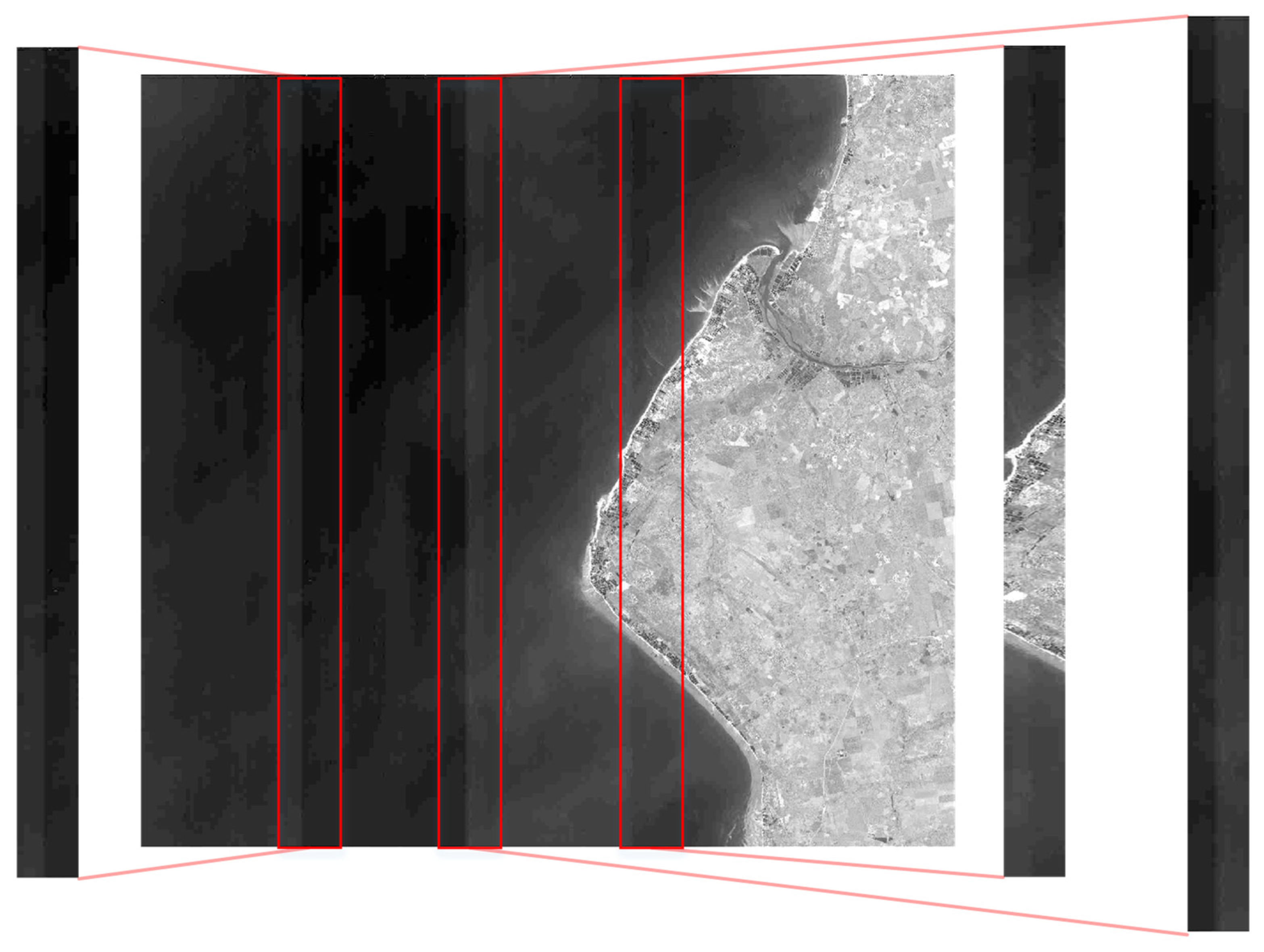
Figure 1. Images with stripe noise.
Remotesensing 14 00873 g001
Figure 2. Flowchart of research method.
Remotesensing 14 00873 g002
Figure 3. Flowchart of stripe noise simulation method.
Remotesensing 14 00873 g003
Figure 4. The LSND network structure framework.
Remotesensing 14 00873 g004
Figure 5. Flowchart of non-maximum suppression of linear objects method. The left side shows the original image, the detection result without linear non-maximum suppression, and the detection result after linear non-maximum suppression; on the right side, the red part, the green part, the blue part, and the yellow part, respectively, represent steps (1), (2), (3), and (4).
Remotesensing 14 00873 g005
Figure 6. Flowchart of Large-scale image stripe noise detection.
Remotesensing 14 00873 g006
Figure 7. The comparison between the simulated and real images with stripe noise: (a) represents the simulated images with stripe noise; (b) represents the real images with stripe noise.
Remotesensing 14 00873 g007
Figure 8. Comparison between the loss curves: (a) comparison of the loss function curves for the training set; (b) comparison of the loss function curves for the validation set; (c) comparison between the loss curves of LSND and LS-YOLOv4 for the training and validation sets.
Remotesensing 14 00873 g008
Figure 9. Comparison of the evaluation indicators: (a) precision curves; (b) recall curves; (c) F1-score curves; and (d) AP curves.
Remotesensing 14 00873 g009
Figure 10. Comparison between the evaluation curves of images with different sizes: (a) precision curves; (b) recall curves; (c) F1-score curves; and (d) AP curves.
Remotesensing 14 00873 g010
Figure 11. Comparison of the detection performance of the models.
Remotesensing 14 00873 g011aRemotesensing 14 00873 g011b
Figure 12. Detection of stripe noise in (a) large-sized images and (b) small-sized images using the LSND-based model.
Remotesensing 14 00873 g012aRemotesensing 14 00873 g012b
Figure 13. Schematic diagram of detection of stripe noise in real images.
Remotesensing 14 00873 g013
Figure 14. Schematic diagram of detection of stripe noise in entire images. The left side represents entire images, and the blue lines on the right side represent the visual detection results.
Remotesensing 14 00873 g014aRemotesensing 14 00873 g014bRemotesensing 14 00873 g014c
Table 1. The current research status of stripe noise detection.
ReferencesDetection Method
Destriping CMODIS based on the FIR method [5]The wavelet transform is used to detect the singularity of the signal, and the periodic distribution of the stripe noise in the wavelet coefficients is used to detect the position of the stripe noise.
Terra MODIS band 5th stripe noise detection and correction using the MAP-based algorithm [6]The gradient of each pixel in each direction is calculated. Then, the noise pixels in the stripe noise image are extracted based on the threshold, to finally realize the detection of stripe noise.
Extremely sparse stripe noise removal from non-remote-sensing images using straight-line detection and neighborhood grayscale-weighted replacement [7]Preselected stripe noise lines are detected using a local progressive probabilistic Hough transform. Subsequently, the real stripe noise lines are screened from the detected lines according to the features of the grayscale discontinuities.
Remote sensing image stripe detection and destriping using the joint sparsity constraint with iterative support detection [8]The ℓw,2,1-norm is used to characterize the joint sparsity of the stripes, and iterative support detection (ISD) is applied to calculate the weight vector in the ℓw,2,1-norm, which shows the stripe position in the observed image.
Noise detection and image denoising based on fractional calculus [9]The noise detection method determines the noise position by the fractional differential gradient; it achieves detection of the noise, snowflake and stripe anomalies by utilizing the neighborhood information feature of the image and the contour and direction distribution of various noise anomalies in the spatial domain.
Table 2. Information on the stripe noise of an image (line labels). Each row represents the category, center point coordinate, and length of the stripe noise in the image.
CategoryCenter Point XCenter Point YLength H
0477320640
0615320640
0625320640
Table 3. Stripe noise information in the form of a bounding box generated based on Table 2 (box labels).
CategoryCenter Point XCenter Point YWidth HLength H
04773202640
06153202640
06253202640
Table 4. Comparison of the performance of different algorithms on the validation set. In the table, each row represents the best results of an algorithm under a certain evaluation index in all epochs of evaluation; the numbers in bold represent the best value in each column; GT represents the number of stripe noises to be detected.
AlgorithmBackboneSizeGTPrecision
Rate (%)
Recall Rate (%)F1-Score
Rate (%)
AP
Rate (%)
LSNDCSPDarkNet53640242098.7493.8596.0992.07
LS-YOLOv4CSPDarkNet53640242089.9893.5691.6088.84
YOLOv4CSPDarkNet53640242059.4362.6556.2549.08
RetinaNetResNet50-FPN640242097.6616.2627.7014.56
FCOSResNet50-FPN640242066.4815.7923.967.36
Table 5. Performance comparison between the LSND and LS-YOLOv4 for images with different sizes. In the table, each row represents the best value of an algorithm under a certain evaluation index in all epochs of the evaluation: GT represents the number of stripe noises to be detected; the numbers in bold represent the best value in each column; and the italic bold numbers indicate the best value for the small-sized images.
AlgorithmBackboneSizeGTPrecision
Rate (%)
Recall Rate (%)F1-Score
Rate (%)
AP
Rate (%)
LSNDCSPDarkNet53640242098.7493.8596.0992.07
LS-YOLOv4CSPDarkNet53640242089.9993.5691.6088.84
LSNDCSPDarkNet53641839094.2886.0389.9378.86
LS-YOLOv4CSPDarkNet53641839079.2288.8883.1980.21
Publisher’s Note: MDPI stays neutral with regard to jurisdictional claims in published maps and institutional affiliations.