Article

Compact Midwave Imaging System: Results from an Airborne Demonstration

1
Applied Physics Laboratory, Johns Hopkins University, Laurel, MD 20723, USA
2
Carr Astronautics, Greenbelt, MD 20770, USA
3
NASA Goddard Space Flight Center, Greenbelt, MD 20770, USA
*
Author to whom correspondence should be addressed.
Remote Sens. 2022, 14(4), 834; https://doi.org/10.3390/rs14040834
Submission received: 6 January 2022 / Revised: 3 February 2022 / Accepted: 5 February 2022 / Published: 10 February 2022
(This article belongs to the Section Atmospheric Remote Sensing)

Abstract

:
The Compact Midwave Imaging System (CMIS) is a wide field of view, multi-angle, multi-spectral pushframe imager that relies on the forward motion of the satellite to create a two-dimensional (2D) image swath. An airborne demonstration of CMIS was successfully completed in January–February 2021 on the NASA Langley Research Center Gulfstream III. The primary objective of the four-flight campaign was to demonstrate the capability of this unique instrument to perform stereo observations of clouds and other particulates (e.g., smoke) in the atmosphere. It is shown that the midwave infrared (MWIR) spectral bands of CMIS provide a unique 24/7 capability with high resolution for accurate stereo sensing. The instrument relies on new focal plane array (FPA) technology, which provides excellent sensitivity at much warmer detector temperatures than traditional technologies. This capability enabled a compact, low-cost design that can provide atmospheric motion vectors and cloud heights to support requirements for atmospheric winds in the 2017–2027 Earth Science Decadal Survey. Applications include day/night observations of the planetary boundary layer, severe weather, and wildfires. A comparison with current space-based earth science instruments demonstrates that the SWIR/MWIR multi-spectral capability of CMIS is competitive with larger, more expensive instrumentation. Imagery obtained over a controlled burn and operating nuclear power plant demonstrated the sensitivity of the instrument to temperature variations. The system relies on a mature stereoscopic imaging technique applied to the same scene from two independent platforms to unambiguously retrieve atmospheric motion vectors (AMVs) with accurate height assignment. This capability has been successfully applied to geostationary and low-earth orbit satellites to achieve excellent accuracy. When applied to a ground-point validation case, the accuracy for the CMIS aircraft observations was 20 m and 0.3 m/s for cloud heights and motion vectors, respectively. This result was confirmed by a detailed error analysis with analytical and covariance models. The results for CMIS cases with underflights of Aeolus, CALIPSO, and Aqua provided a good validation of expected accuracies. The paper also showed the feasibility of accommodating CMIS on CubeSats to enable multiple instruments to be flown in a leader–follower mode.

Graphical Abstract

1. Introduction

Atmospheric motion vectors (AMVs) have long provided an important component of the global observing system for tropospheric winds [1]. The 2017–2027 Earth Science Decadal Survey (ESAS 2017) [2] identified 3D winds including AMVs as a “targeted observable” to advance research objectives in atmospheric dynamics, severe weather, wildfire, and hydrology. The community increasingly recognizes that study of atmospheric dynamics is essential to the understanding of cloud-climate and cloud-precipitation processes, as discussed in the recommendation: “global measurements of the spatiotemporal (four-dimensional) evolution of large-scale horizontal wind vectors are urgently needed” [3]. The Compact Midwave Imaging System (CMIS) project represents an effort to address these objectives with a compact, low-cost sensor that enables flexible accommodation on CubeSat or as hosted payloads on small satellites. CMIS employs a robust stereo technique with accurate height assignment [4] to provide wide field of view (FOV), multi-angle observations of AMVs during the day and night over cloud-covered regions of the Earth (more than 60% coverage of the globe). This capability would produce vector winds resolved in 3D along each orbit, effectively complementing clear-air wind measurements yielded by LIDAR, to achieve a synergistic architecture for a global 3D wind characterization.
Until recently, only cryogenically cooled detector technologies such as InSb and HgCdTe, which require detector temperatures < 80 K were available for midwave infrared (MWIR) sensing. The detectors from CMIS are made from the newly available and continually improving high-operating temperature (HOT) detector technology in the 2–5-μm spectral range based on Type II Superlattice (T2SL) detector structures. These detectors are able to deliver similar performance at operating temperatures near 150 K as those made from the incumbent InSb and HgCdTe technology. The significant increase in operating temperature allows for smaller, lighter, and lower-power Stirling cycle coolers which are consistent with the resources available from a CubeSat. This paper presents the initial results of an airborne flight test carried out in early 2021, as well as provides a brief description of the CMIS design. The paper also describes how CMIS could provide a low-cost option for a future space mission.

2. Materials and Methods
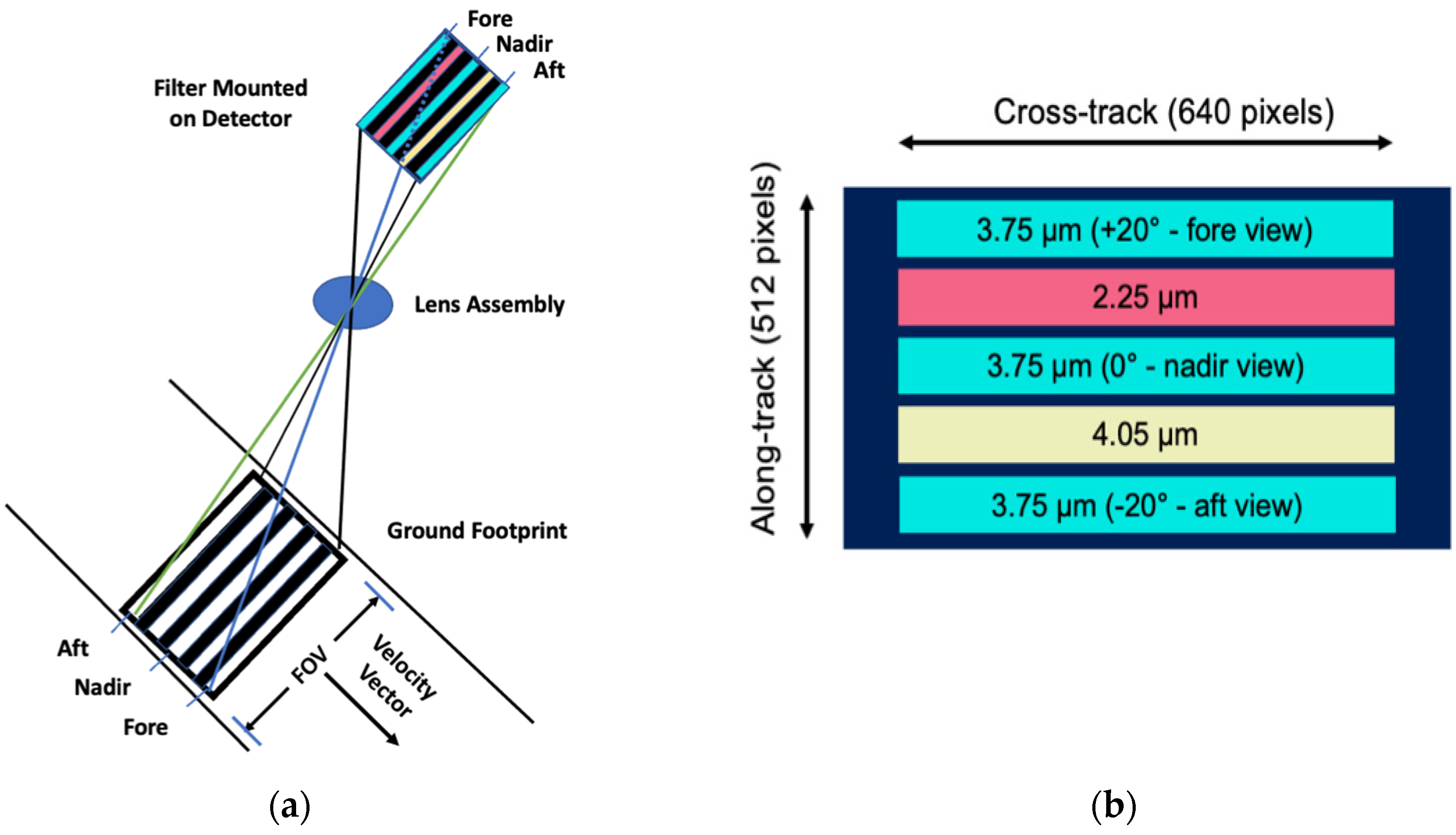
2.1. Instrument

CMIS is a pushframe imager with a single lens assembly that relies on the forward motion of the satellite (or aircraft) to create a two-dimensional (2D) image swath (Figure 1a). The optical design of pushframe imagers is based on a set of passband filters inserted into the optical path directly over a focal plane array (FPA) such that each filter stripe maps into a unique row (line), or a continuum of rows, on the array. As shown in Figure 1b, the CMIS filter design includes three stripes at 3.75 μm to provide fore (+20°), nadir (0°), and aft (−20°) views, plus two stripes at 2.25 μm and 4.05 μm in between. A given wavelength stripe on the filter covers 32 rows of pixels on the FPA at the same wavelength in order to allow for time-delay integration (TDI) to build up signal if needed to image dim targets.
As the satellite moves along its orbital track, the imager takes samples of pixels in a cross-track (XT) swath and maps each pixel from each stripe to a unique spot on the ground. This is shown in the CMIS ‘snapshot’ in Figure 2a. As the satellite (or aircraft) moves forward, the instrument builds up a continuous ground swath for each stripe, with different relative coverage times by each stripe for a given swath. At typical orbital speeds ~7.7 km s−1 in low-earth orbit [6], the nadir and aft 3.75-μm stripes image a given ground swath at 20 s and 40 s, respectively, after the time that imagery for the same area was collected by the 3.75-μm fore stripe. This design allows us to measure the apparent change in position of a cloud between the fore and nadir views and again between the nadir and aft views, as shown in Figure 2b.
These apparent changes in position, referred to as disparities, are used to derive atmospheric motion vectors (AMVs) and cloud-top heights (CTHs). The first step in the process is to perform geolocation and apply a calibration to derive radiances for each stripe. Radiances are then used to perform pattern matching for clouds and terrain between the fore and nadir, and the nadir and aft images. Texture, shape, and size of the individual cloud elements contribute to the correlation between patterns in different images used to identify a positive match. After cloud elements are matched between multiple images, disparities can be derived. The component of the disparity in the XT direction relates directly to XT wind speed, although CTH is needed to correctly calculate the velocity. Disparities in the along-track (AT) direction contain information about both the CTH and AT wind, which are difficult to separate. An independent view from another platform is needed to resolve this ambiguity. Nadir views in two platforms in a leader–follower formation together with times of observation for both platforms can be used to determine the wind velocity in the AT direction. This constrains the fraction of AT disparity due to AT winds, thereby allowing retrieval of CTH. Given CTH, XT winds can be retrieved for the given XT disparities. This method is very simple conceptually, but numerical methods are required to perform optimal fits over large scenes. These methods are described in Carr et al. [4] and adapted for an aircraft as described below.
Figure 3 presents the three spectral bands chosen for the CMIS instrument, superimposed on a MODTRAN atmospheric transmission spectrum. The bands are located in spectral windows where the atmosphere has high transmission. The band at 3.75 µm provides day and night (24/7) images for stereo sensing. The band at 4.05 µm can be used to derive temperatures, including those for land and sea surfaces, volcanic plumes, and wildfires. Finally, the band at 2.25 µm, which is dominated by solar reflection, provides high-spatial-resolution cloud reflectivity data that will aid in the determination of AMVs, cloud/surface phenomenology discrimination and removal of the daytime solar signal from the 4.05-µm band. The 2.25-µm band is also useful for detecting hot wildfires with fewer saturated pixels than the other two bands, due to blackbody physics and a narrow bandwidth.
The 3.75-μm band was chosen to collect multi-angle observations for CMIS for several reasons. In general, multiple choices within the midwave infrared (MWIR; 3–5 μm) or longwave infrared (LWIR; 7–14 μm) spectrum are capable of providing day/night observations, which are needed to meet science requirements specified in the 2017–2027 ESAS. To meet sensitivity requirements, the CMIS detector requires cooling to 150 K at 3.75 μm, which is much warmer than that required for LWIR wavelengths (e.g., 12 μm). A relatively warm operating temperature is important for keeping the overall power draw low for the instrument. Finally, a band at 3.75 µm provides higher spatial resolution than a potential 12-μm band on a pixel-by-pixel basis for the same size lens due to the smaller diffraction blur at shorter wavelengths. The spatial improvement is nominally ~3×, since 3.75 μm is more than a factor of three shorter than 12 μm.
Midwave-infrared channels (3–5 μm) have become a staple of Earth remote sensing with proven capabilities on GOES, POES (AVHRR), JPSS (VIIRS), and Terra/Aqua (MODIS), among others. VIIRS and MODIS use HgCdTe detectors that require cooling down to cryogenic temperatures (80 K). MISR relies on an uncooled CCD which acquires images in the visible and provides a stereo capability like CMIS. Table 1 shows the comparison between measured performance for CMIS and specifications for VIIRS, MODIS, MISR, and ASTER.
As described in Table 2, the mass of the instrument is 3 kg with an average power draw of 8 W (20 W peak power after initial turn on). The overall instrument size is 20 × 10 × 10 cm for the optical instrument and 9 × 9 × 9 cm for the electronics. The measured performance of CMIS is competitive with, yet much lower in cost and smaller in size, weight, and power (SWaP) than any of these instruments.
Figure 4a presents an overview of the CMIS instrument design, showing the placement of the ceramic pallet, the filter over the FPA, lens assembly, and cryocooler. The five-zone filter is installed immediately above the FPA (Figure 4b). The system has full-frame readout of the FPA with the five regions of interest extracted, one region per filter zone. The only moving parts of CMIS are the cryocooler and calibration mechanism.

2.1.1. Focal Plane Array (FPA)

The FPA has the capability to operate at a frame rate synchronized to the ground advance of one pixel, ~13 Hz for a 415-km orbit. Full 640 × 512-pixel image frames are acquired by the camera electronics, which then selects five lines for output, one for each filter stripe. The epoxy that holds the filter stripes together creates low optical transmission zones near the margin of the stripes, leaving 32 unobstructed lines available for processing by the camera electronics. The test flights demonstrated that the calibration for the CMIS detector is very stable with time. Gain coefficients measured more than a year prior yielded brightness temperatures accurate to ±1 K.
The focus of the current paper is to demonstrate multi-angle observations from the 3.75 µm bands for retrieving stereo cloud heights and AMVs. The stereo imaging technique requires only relative intensity measurements from a cloudy scene, as the algorithm tracks and matches the cloud patterns to determine their disparity with respect to the ground. However, calibrated radiances from the CMIS channels will enable additional retrievals of cloud and surface properties, such as temperature and fire intensity. A multispectral analysis of collocated 2.25, 3.75, and 4.05 µm measurements can determine the relative contribution between the reflected solar and thermal blackbody emissions from the atmosphere. A future effort will be devoted to evaluate a solar-corrected brightness temperature at 3.75 µm. During daytime collections, the radiance in the 2.25-µm band will be used to separate the reflected and thermally emitted component of the incident light at 3.75 µm [7]. We can also take advantage of the fact that each temperature has a unique ratio of blackbody radiance at different wavelengths. The ratio of the signals in the 4.05-µm and 3.75-µm bands can thus be used to further refine the temperature measurement. Temperature estimation will be the focus of a future study.

2.1.2. Optics

To meet instrument performance goals, a custom high-speed, wide-field, imaging lens with five elements was developed. A 13-mm focal length provides a 50° × 40° field of view over the detector at a focal ratio of f/1.2. An achromatic design allows all three bands to be captured on the same image plane, which enables the lens to be set to a single focus position.

2.1.3. Cryo System

The pallet holding the FPA, filter, and optics is cooled to 150 K, so as to minimize thermal emissions from the lens assembly. Although the outer edge of the lens assembly is exposed to the ambient environment, cryocooling is expected to reduce stray light, which is crucial to maintain sensitivity at cold temperatures (i.e., T < 240 K). The cryocooler coldfinger is coupled to the pallet by a three-spoke copper strap.

2.1.4. Dewar

CMIS has a vacuum dewar to allow operation of the instrument in an aircraft environment.

2.1.5. Radiometric Calibration Mechanism

Pixel offset corrections are obtained by periodic views of a thermally-controlled, high-emissivity calibration surface. The CMIS airborne instrument employed a motorized paddle system with a black-painted, large-area thermo-electric (TE) cooler as the calibration surface. The calibration mechanism implements a two-point non-uniformity correction (NUC) at temperatures of 10 °C and 20 °C, which provides sufficient dynamic range to enable accurate measurement of thermal signatures of targets that were considerably colder than the low NUC source. To improve packaging within the CubeSat, a change to a linear mechanism is anticipated for the spaceflight model.

2.1.6. Electronics

CMIS camera electronics (Detector Board, Digital Board, and Power Board) were implemented in a small form-factor chosen specifically for CubeSat compatibility. Components were selected and the boards were laid out to accept either low-cost commercial components for the airborne model or their high-reliability equivalents for the spacecraft model.

2.2. Flight Collections

An airborne demonstration of CMIS was conducted in January–February 2021 on the NASA Langley Research Center (LaRC) Gulfstream-III with four round-robin flights out of LaRC. The first flight on 22 January 2021 was an ‘engineering flight’ designed to demonstrate that the airborne instrument setup collected and successfully stored data. The objective of the engineering flight was to verify that the flight procedure allowed sufficient time for the instrument to reach its operating temperature of 150 K and that the various instrument commands were executed correctly by the support equipment and software on aircraft. The flight plan for the engineering flight was chosen to cover relatively long, linear ground features to allow the calculation of a high fidelity (pixel-level) lens distortion model. Another objective of this flight was to collect measurements from both cold and warm targets to verify that the instrument meets its designed dynamic range. All objectives of the engineering flight were achieved.
Three science flights were conducted on 27 January, 29 January, and 8 February as shown in Figure 5. The case studies and aircraft holds analyzed for this effort are depicted with arrows. Each hold consists of a racetrack flight pattern intended to cover the scene with two passes (e.g., Hold D1 and D2, or collectively Hold D). The red line segments and boxes show the overpasses of satellites used for validation. Selected cases were limited to periods with stable flight profiles without significant yawing maneuvers or turbulence.
Each flight was designed to collect on cloud features during specific underflights of earth-observing satellites. For example, the purpose of Science Flight #1 was to collect on daytime marine and land stratocumulus and to underfly CALIPSO and MODIS.
As discussed below, the capability to produce AMVs and CTHs for the free troposphere and PBL from CMIS data is demonstrated with these aircraft flights. The flights successfully achieved their primary objectives, which were to show that the sensitivity of the focal plane array and the quality of the images met requirements specified for the instrument (Table 3).

2.3. Geolocation

Conventional imaging generally requires an intricate co-registration process to perform pixel-to-pixel matching for pushframe imagery taken at different rows on an FPA. This procedure is especially critical for images collected from an aircraft due to the continual yawing/pitching motions, even during straight, and level flight on autopilot. Figure 6 depicts the data collection and processing pipeline for the aircraft flights.
Because changes in aircraft attitude can artificially skew features by hundreds of pixels, which complicates stereo matching, it was necessary to track the position and orientation of the CMIS camera relative to an earth-fixed frame. This was done by rigidly attaching a high precision NovaTel Inertial Measurement Unit (IMU) to the camera mounting plate and calculating the global camera pose at the acquisition of each camera frame.
The initial engineering flight was used to geometrically calibrate the camera by matching 150 key points in each pushframe view to known points on the ground. This helped determine the fixed offset and rotation matrices between the IMU and the CMIS sensor, as well as the camera lens distortion parameters. When combined with the IMU position and orientation, pixels in the camera image plane could therefore be projected onto the WGS-84 ellipsoid to provide motion-compensated, geo-registered imagery for stereo matching.
Position and orientation data from the primary NovaTel IMU was used to analyze Science Flights #1 and #2. However, data from a backup IMU was used to analyze Science Flight #3. Approximately 90 min into the four-hour flight (23:00Z on 8 February 2021), the primary IMU lost GPS lock and failed to provide a "fine steering" solution. Efforts to correct the problem in-flight were not successful. Fortunately, the CMIS imager continued to acquire imagery during the primary IMU dropout, and a logging application saved position and orientation data from a navigation IMU attached to the NASA Gulfstream III aircraft’s ARINC-429 bus. The primary and backup IMU poses were aligned to each other by shifting the orientation data streams in time during the first part of Science Flight #3 when both sources of data were available, and verifying that the geo-registered images matched before the primary IMU dropout. To remove the chance for an abrupt data transition between the two IMUs at the 23:00Z boundary, only the backup IMU was used to geo-register Science Flight #3.

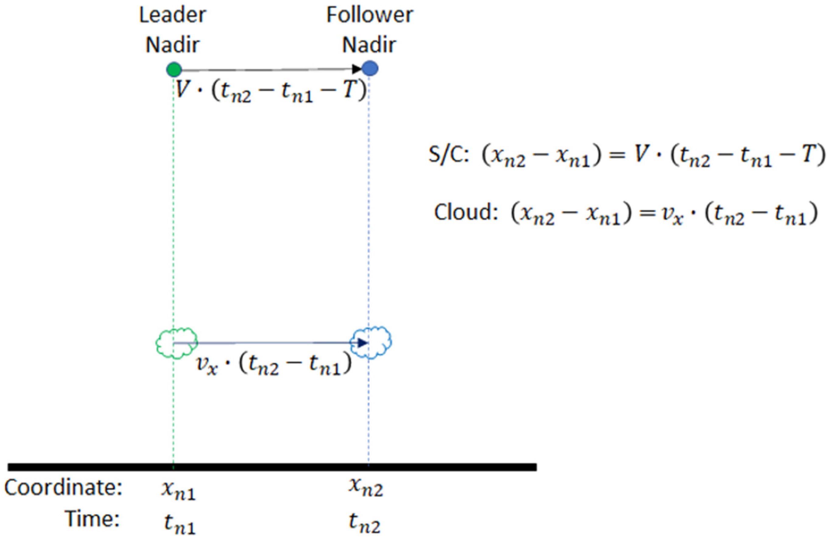
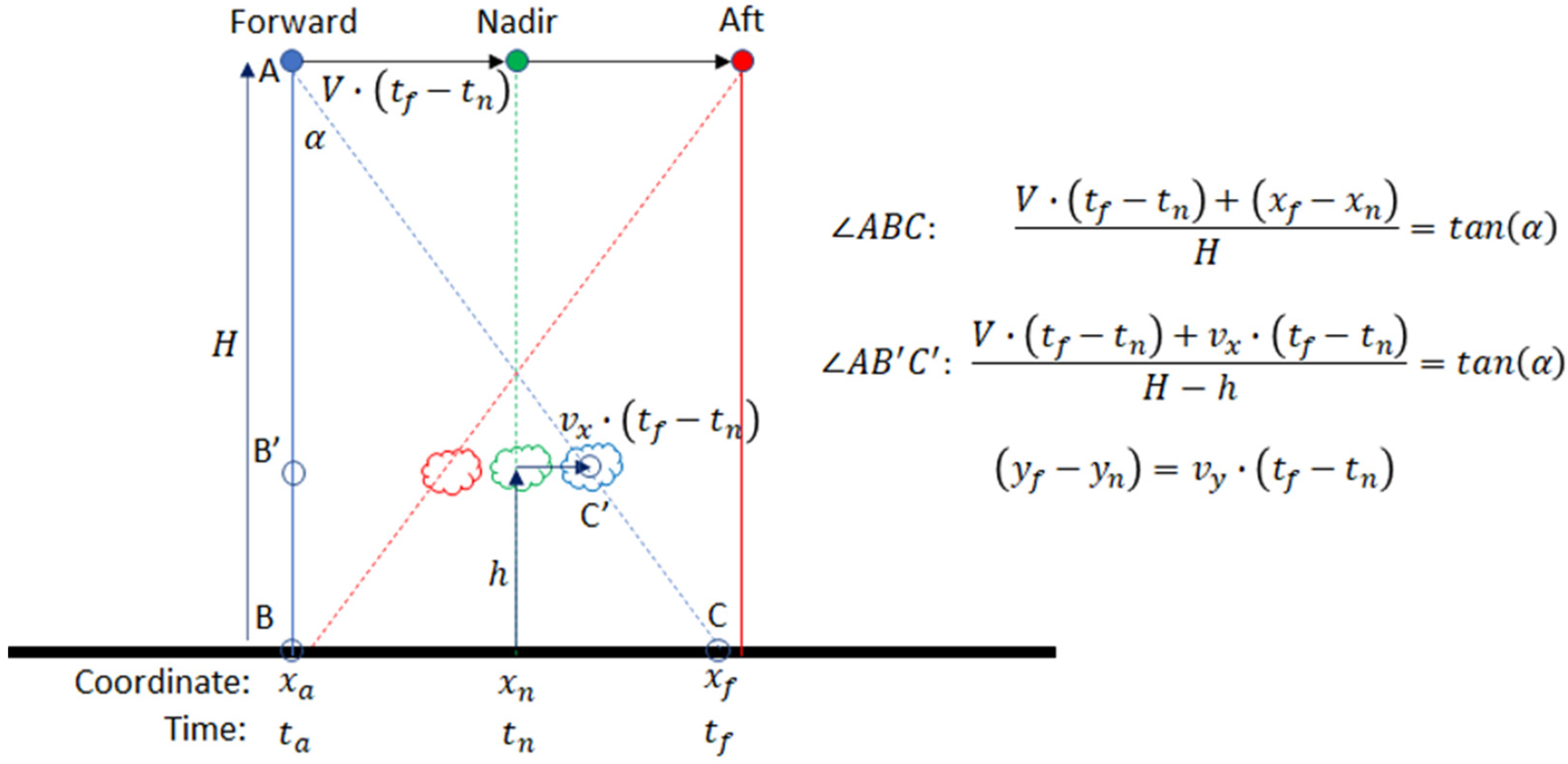
2.4. Stereo Technique

The CMIS stereo-winds are based on stereo-wind methods successfully applied in several multi-angle, multi-platform cases [4,8]. Templates are extracted from the CMIS nadir-looking view on a regular grid. Retrieval sites are generally oversampled with respect to the template size, so with an N × M pixel template and 2:1 oversampling, wind retrieval sites would be arranged in a lattice sampled every (N/2) × (M/2) pixels. Each feature template is searched for in both forward- and aft-looking views using a normalized cross-correlation (NCC) algorithm to find matches. Thus, the algorithm does not require absolute radiometric accuracy, but only the relative intensity variations from a feature pattern. The apparent displacement of the feature, or disparity, is interpolated for sub-pixel resolution and tested for significance using the peak NCC value. The fundamental premise of this method is that a translation accurately describes the relationship between the template feature and its match in another view. This premise can be violated when the aircraft experiences turbulence or submits to frequent control inputs during powered flight. To mitigate the adverse impact on feature matching, the imagery is first pre-rectified so that it is uniformly sampled on a plane that is tangent to the WGS-84 ellipsoid at the center of the collect. AT and XT coordinate axes are defined along and across the mean direction of flight. This worked well to improve matching efficiency to yield larger numbers of forward– and aft–nadir matching pairs, but only for cases and holds where the flight trajectory and aircraft attitude were relatively smooth. In other cases, the motion was not sufficiently well compensated in pre-rectification to allow gathering large sets of matches. These types of issues will largely disappear for a space flight.
There are individual AT and XT components for each of the two fore–nadir and aft–nadir disparities, for a total of four scalar measurements at each retrieval site, from which to estimate a horizontal wind velocity with AT and XT components and a height above the WGS-84 ellipsoid, for a total of three states. The XT component of disparity can be considered mostly due to XT wind velocity as there are typically several tens of seconds in time between acquisitions of the same feature in the forward- or aft-views (i.e., measurement spacing).
Table 4 shows the small difference in measurement spacing, defined here as the time for the aft look vector to intersect the fore look vector at a nominal cloud retrieval height (1000 m) above the ellipsoid, between an aircraft and satellite. Our calculations assumed a linear path for the aircraft and a curved path for the satellite to account for the earth’s curvature. The measurement spacing at a given altitude for an aircraft depends on its ground speed, which varies based on the wind velocity at cruise altitude. For our purposes, the speed of a satellite in a circular orbit can be considered as relatively constant.
The AT component of disparity can be considered mostly due to a combination of geometric parallax and AT wind velocity. It is not possible to separate the geometric height due to parallax and AT wind without either additional observations or a prior assumption about one of them. This is known as the AT ambiguity. Our retrieval algorithm implements a non-linear least-squares solution to the problem of fitting the best three states (two wind plus height) to the two disparities given the trajectory of the aircraft and the sampling times. A cost to deviate from an a priori wind is added to the cost function to be minimized with weightings so that the cost is negligible to deviate XT but prohibitive to deviate AT. This effectively constrains the AT wind to equal the prior value and leaves the height free to fit the data. The result is correct only if the prior value is correct. Alternatively, a prior height can be set and both wind components left free to fit the data. The original intent was to fly two passes over each collection target and combine observations from both passes to jointly estimate AT wind. However, the XT winds tended to carry cloud features out of the narrow swath when revisited, so this approach was largely unsuccessful.
For a single-pass solution, four scalar disparity observations per site with a prior value for either AT wind or height are sufficient to overdetermine the three states, so the residuals after fitting can be used to quantify conformance of the observations to the model. This allows discrimination between good solutions that are properly interpreted as jointly retrieved winds and stereo heights and meaningless ones. We apply a maximum absolute difference (MAD) filter, at a Gaussian-equivalent 3-sigma confidence level, to identify anomalously large residuals in the population of all residuals to discriminate between good (meaningful) and bad (meaningless) solutions with respect to the retrieval model.

3. Results

The objective of the airborne science flights was to assess the performance and capability of CMIS of producing science-quality AMV and cloud height observations under different scenes. The overall flight plan was to collect the data on both clear and cloudy scenes to characterize the sensor’s properties.

3.1. Imagery

The scenes presented in this subsection highlight a few examples of the high-quality imagery collected by CMIS. Figure 7 depicts a scene in Florida (Case M) from science flight #2 in which an agricultural field is undergoing a controlled burn. The images show calibrated, geo-referenced irradiance for the three CMIS spectral wavelengths. Since the aircraft was not constrained to fly along cardinal direction, the data swath was rotated relative to a standard latitude–longitude Mercator grid. The images required approximately 65 s to collect. The remaining images will be presented on an AT-XT grid for convenience. The undulations at the boundaries of the image result from the aircraft motion during the autopilot course corrections.
Some of the radiances from the 3.75- and 4.05-µm bands are saturated in the high temperature regions associated with smoke and gases adjacent to the flames, because of a long integration time used in the data acquisition. Fewer 2.25-µm pixels are saturated because of the narrow bandwidth (50 nm) centered on 2.25 µm and the temperature of the fire. Dual gains can be implemented in the future to reduce and potentially eliminate saturated pixels.
Figure 8 presents calibrated radiance from the St. Lucie Nuclear Power Plant on the east coast of Florida (Case N) on 19 January 2021. As expected, radiance is higher at 3.75 µm than at 4.05 µm due to higher reflectivity at the shorter wavelength. The overall scene contrast at 3.75 µm is larger because of greater reflectivity and higher quantum efficiency at that band than at 4.05 µm. Temperature differences indicated by differences in radiance for waters near the power plant are quite visible at both wavelengths, particularly for a single, wide warm-water outlet and two narrow cold-water inlets. Warming of the ocean waters adjacent to the St. Lucie nuclear power plant is indicated by the line of enhanced radiance extending horizontally from the warm water outlet. Cooler temperatures of the Atlantic Ocean are also clearly evident near the top of the image.
The radiance of Earth includes roughly equal contributions from reflected and emitted radiation in the MWIR. At night, MWIR bands have sufficient signal to directly estimate temperature for such terrestrial features as clouds, ocean, and terrain. During the day, temperature can still be extracted, but the retrieval requires additional processing to remove reflected solar radiance [7].

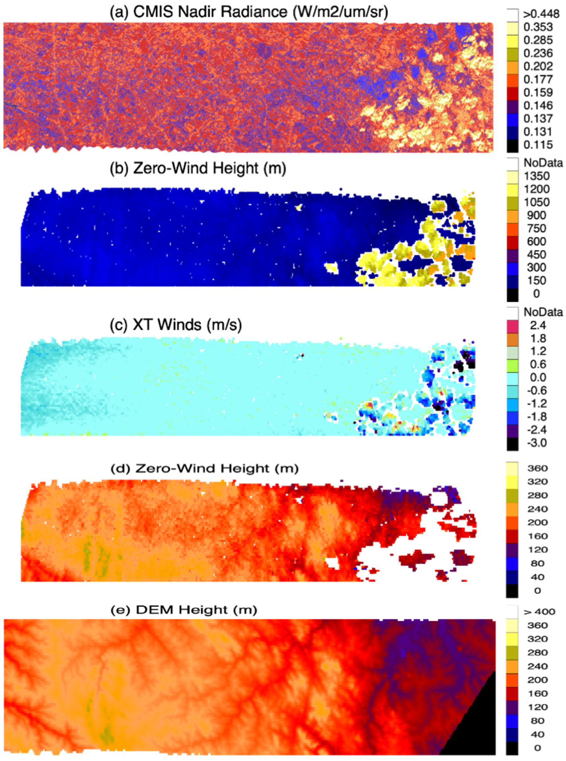
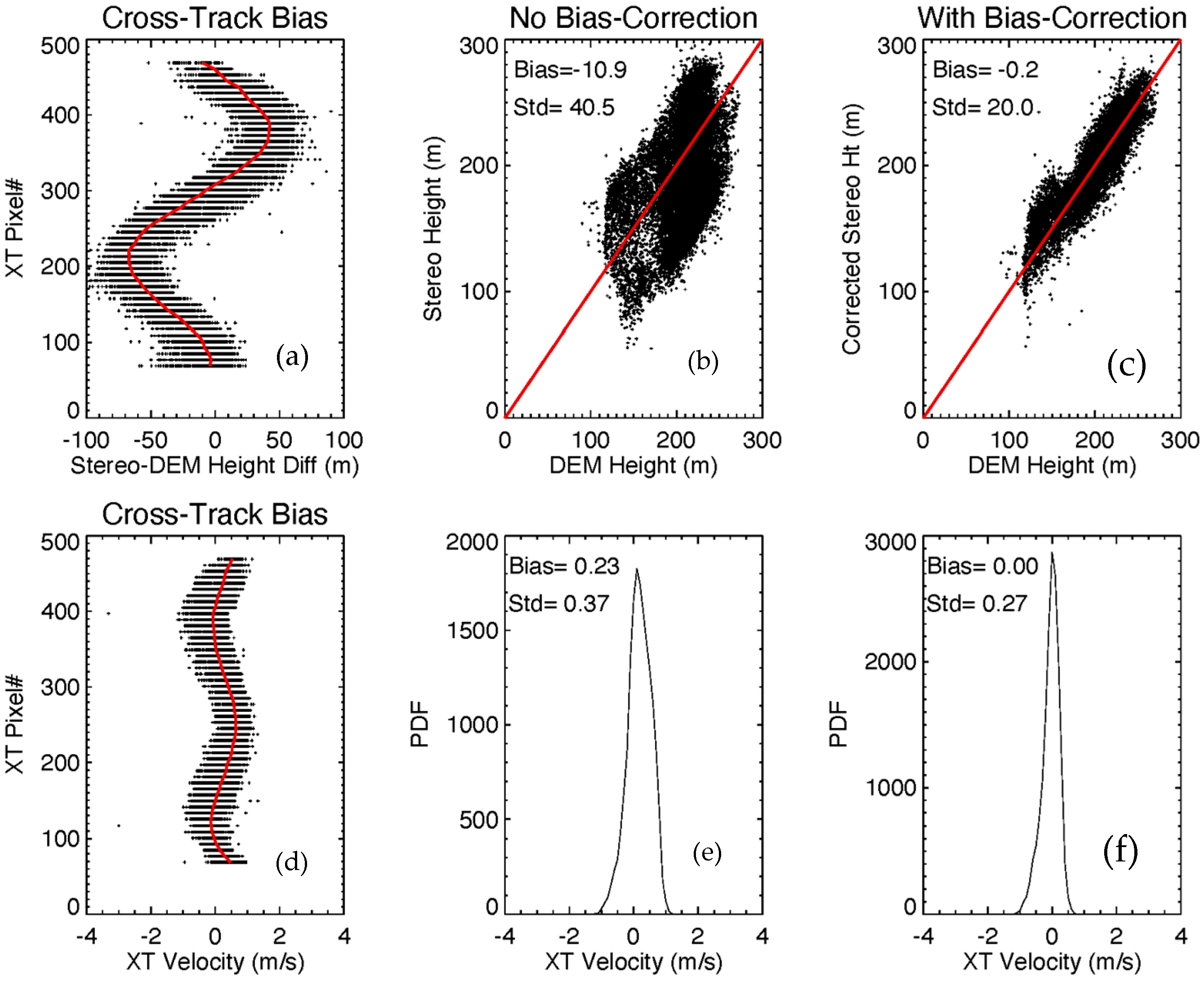
3.2. Ground Point Validation

The Hold F flight contains mostly clear-sky land pixels over farmland in the vicinity of Durham, NC during the day. This case offers the opportunity to validate against static targets (i.e., terrain) with known altitudes. The aircraft made two passes over the collection area, but a readout error affected imagery from the first pass (Hold F1), rendering only the second (F2) useable.
The ground sampling for this case is 12.2 m (AT) × 22.8 m (XT) per pixel and the time difference between forward-nadir and aft-nadir looks is a nearly constant ±19 s. Feature templates of 16 × 16 pixels were used to obtain disparity matches at 20373 sites. The retrieval model solved for height and velocity with prior AT velocity set at zero, as it should be for the ground.
Figure 9a features radiance measurements from the 3.75-µm nadir stripe where the aircraft route of flight was from left to right. The radiance across the left two-thirds of the image is fairly uniform due to flat terrain, as indicated by the zero-wind heights shown in Figure 9b. The radiances in the right 1/3 of the image are higher due to the high reflectivity of clouds in the MWIR. Under the assumption of zero AT winds, the XT winds (Figure 9c) were retrieved with values for this case ranging between −3.0 and 2.4 m/s. The bias-corrected XT winds are very close to zero in the no-cloud region (i.e., the terrain is not moving) as they should be. We also note that patterns of what appears to be mass divergence with positive XT winds adjacent to negative XT winds in the cloudy region (Figure 9c). Figure 9d presents the zero-wind heights only for heights below 400 m in order to facilitate comparison with digital elevation map (DEM) heights (Figure 9e). The white area in Figure 9d (i.e., no data) is the region obscured by clouds. Comparison between Figure 9d,e shows that the CMIS stereo retrieval replicates the small 50- to 100-m variations in terrain height well.
Figure 10 shows a histogram of all retrievals passing the quality criteria. The clouds clearly separate from the clear-sky ground-points, which can be classified by their retrieved height (<500 m) and speed (<5 m/s). The ground-point class consists of 16,518 sites also meeting the retrieval quality criteria. The retrieved heights of ground points are then compared to the USGS one-arc-second digital elevation model (DEM) and the retrieved XT velocity is compared to zero.
The next step is to evaluate the statistical performance of CMIS retrievals for Hold F. Figure 11a–c show a point-by-point comparison between the initially retrieved stereo heights and the DEM from Figure 9e. Since the DEM represents height above the geoid, we subtracted the geoid height above the WGS-84 ellipsoid, which is equal to −32 m at the center of the collection, to represent the terrain height above the ellipsoid. Finally, the DEM is averaged to a scale, which is comparable to that of the templates.
Figure 11a,d show the XT residuals for the initial stereo heights and XT winds, respectively. These are a systematic bias that can be determined empirically as a function of the XT pixel number and removed from the initial stereo height and XT wind retrievals. We see in Figure 11b and e that the biases for the uncorrected CTH and XT winds are −11 m and 0.23 m s−1, respectively, which affects their overall accuracy. When the biases are corrected, the standard deviations reduce to 20.0 m and 0.27 m s−1 (Figure 11c,f) for the CTH and XT winds, respectively. Thus, systematic error compensation is needed to achieve the best results for this case.
The leading hypothesis for the origin of the systematic errors is imperfect optical calibration initially done in the laboratory and adjusted in flight using mapped features such as roads. Our analysis of differences between stereo and DEM heights for ground points demonstrates a methodology that can be used in future space flights for geometric calibration or validation.
A scatterplot of XT wind vs. zero-wind height (Figure 12a) reveals an apparent correlation between the two fields. When the data are plotted along the transect shown in Figure 12c, an interesting pattern emerges. The XT winds in the cloudy regions (closed black diamonds) are well correlated (Figure 12b) with the zero-wind cloud-top height (CTH; red triangles). As discussed by Mueller et al. [9], if a platform making stereo observations where the AT wind is not negligible, the errors of retrieved zero-wind stereo CTH and unaccounted AT wind are highly correlated. If the CMIS flight maintains a fixed angle with respect to wind direction and the wind direction does not vary, the wind speed variation would result in a significant AT wind component that induces a stereo CTH error. Since the AT and XT winds are correlated under the fixed directional flight, the AT-CTH error correlation manifests itself as the XT-CTH correlation as seen in Figure 12a,b.
The magnitude of AT winds can be assumed based on the value required to minimize the change in altitude of the cloud-top height. When that assumption was applied for this case (Vat = 2.5 m/s), the XT-CTH correlation disappeared, as shown with the blue-triangle symbols for the wind-corrected heights and XT winds in Figure 12b. The geometry for this situation is illustrated in Figure 13.

3.3. CALIPSO Under-Flight

The Hold D flight path covers a nearly homogenous cloud field above western Pennsylvania nearly simultaneously with an overpass by CALIPSO approximately at 19:00Z on 27 January 2021. For this case, we constrain the wind height using CALIPSO and solve for both wind vector components. This case provides a good example of the synergy between simultaneous aerosol-cloud LiDAR and stereo observations. Figure 14 shows the CMIS retrieval sites for Hold D1 with collocated CALIPSO vertical profiles.
Typically, CALIOP detects clouds and aerosols at lower optical depths than passive imaging, and so CALIOP heights may be higher than those detected with stereo methods [10]. Fixing the mean height for the CMIS wind field at 1400 m based on CALIOP Layer-1 heights, we retrieve CMIS AT and XT winds over the collect with distributions as shown in Figure 15. These are rotated into U (+East) and V (+North) vector components to show mean wind vector values of (3.38, −4.39) m/s.
The Hold-D1 collection has an Aqua overpass approximately an hour earlier at 17:55Z that was used for MODIS and GOES-16 stereo winds to corroborate the CMIS results. A larger domain (41.25 ± 1°, −79.05 ± 1°) is considered since the density of satellite retrievals is much less than those from CMIS and there is approximately a one-hour time mismatch. The distribution of MODIS-GOES stereo winds within this domain is shown in Figure 16. The mean CMIS retrieval of (3.38, −4.39) m/s falls near the most probable satellite U-V winds and its 5.54 m/s speed and mean height of 1400 m also falls near the most probable speed-height combinations.

3.4. Aeolus Under-Flight

The Hold J flight was designed to fly along the track of Aeolus on 8 February 2021 at night. The Atmospheric Dynamics Mission (ADM-Aeolus) Doppler Wind Lidar (DWL) measures the atmospheric wind profile in a horizontal line-of-sight (HLOS) direction 35° from nadir and 90° from the spacecraft velocity. Therefore, the Aeolus measurements are single-component wind profiles along the HLOS. Because of the 35° slant view, each height level of the HLOS wind profile corresponds to a different geographic location, with the higher levels closer to the satellite ground track. This height-dependent geolocation of HLOS winds is evident in Figure 17 and Figure 18.
The Hold J flight is also within the coverage of both GOES-16 and -17. We use the stereo winds from GOES-16 and -17 [8] to set the a priori value of the AT wind for the CMIS retrievals and compare against Aeolus. The first pass (J1) was the most simultaneous to the Aeolus Mie wind retrievals. CMIS was 5 min ahead of Aeolus over Hold J, which was completely cloud covered. Sites for the three sets of retrievals are shown in Figure 17. The sampling scales are quite different, with CMIS densely sampling over a very small patch due to the low altitude of the aircraft (compared to satellites). The GOES stereo winds used a triplet of CONUS scenes centered on 23:36Z from GOES-16 and a doublet of contemporaneous Full Disk scenes from GOES-17. The GOES stereo winds as shown in Figure 17 reveal a cloud layer at 4813 m median height and with median winds resolved along and across the direction of the CMIS flight of 2.76 m/s (AT) and −35.07 m/s (XT). We use 2.76 m/s for the prior value of the AT wind in the CMIS retrieval code and solve for XT wind and CTH at each CMIS retrieval site.
Figure 18 compares AMVs and CTHs from GOES and CMIS against Aeolus Mie winds. There is broad agreement for all three estimates, although Aeolus wind retrievals are biased about 5 ms−1 lower than those retrieved using GOES and CMIS. The XT winds for CMIS match fairly well with G16-G17 stereo winds. We see a local minimum (in magnitude) for both GOES and CMIS near 42.6°N. A similar local minimum appears for Aeolus near 42.7°N. The height retrievals for CMIS (Figure 18b) match the overall shape of those for G16–G17 stereo. We see decreasing CTH between 42.3° and 42.5° for both GOES and CMIS, although the decrease is steeper for CMIS. This may be due to the very fine GSD for the CMIS aircraft payload. CMIS demonstrated good sensitivity to small-scale variability.
The retrieval histograms are shown in Figure 19. The XT wind distribution is quite narrow, and its median value of −35.83 m/s is a good match with the median GOES stereo wind of −35.07 m/s (XT). The distribution of CMIS heights is broader, but the GOES stereo-wind median is in the range toward the upper end.
There are six Aeolus Mie winds in the relevant atmospheric layer. Because the flight line was nearly parallel to the Aeolus track, Aeolus HLOS wind components are opposite in direction to the XT winds from CMIS. Aeolus and CMIS winds are similar but not as well matched as the GOES stereo winds. None of the datasets compared are perfectly aligned in time, location, or scale.

4. Discussion

The CMIS instrument provides three angular views at 3.75 μm, wide-swath coverage and day-night sensing, compatible with a compact 6U-CubeSat design to enable global coverage of the winds and cloud heights in the free troposphere and PBL. Stereo sensing at a wavelength of 3.75 μm permits 24/7 day/night sensing to observe diurnal variation of PBL structures. However, when the clouds are moving in the direction of the spacecraft velocity vector, the stereo technique applied to a single LEO satellite suffers from an aliasing problem in which errors in AT wind and CTH are highly correlated, as is known from MISR [9] and now discussed here. To resolve this ambiguity, stereo imaging requires independent observations from multiple platforms (i.e., joint retrievals). This joint technique can be applied to LEO-LEO platforms or LEO-GEO platforms. It would also be most relevant for a series of CubeSats in a leader–follower configuration (i.e., pearls on a string).
The stereo methodology applied to LEO-LEO satellites is particularly valuable for the polar regions where detection of low-level clouds and semi-transparent clouds is a major challenge for satellite remote sensing. The most accurate method for retrievals at high latitudes could potentially be leader–follower satellites if favorable viewing geometries and optimized spacecraft separation times are maintained. The airborne flights presented here proved the sensitivity of CMIS to detect patterns in PBL clouds for stereo retrievals in the mid-latitudes. Provided sufficient variability in cloud radiance exists for pattern matching, this technique should also work well in the Arctic and Antarctic. Due to frequent turbulence and course corrections, retrievals from an aircraft are much more difficult to do accurately than from space.

4.1. Implications for Notional Spaceflight

The following subsection presents a simple analysis to estimate the accuracy of the retrievals for a spaceflight. These results can be used to specify general requirements for a CubeSat to host a stereo wind sensing mission.

4.1.1. Accuracy

Some very simple geometric relationships can help us estimate stereo wind retrieval accuracies and scale them from an airplane to a spacecraft (our retrieval software using a full fidelity and nonlinear model). Such estimates can be confirmed from the retrieval process, which outputs the three retrieval states (two horizontal wind vector components and the height) along with their 3 × 3 covariance matrix. The latter represents the uncertainties in the states with modeled errors in the input disparities. Figure 20 shows an idealized configuration with a single CMIS flying over the locally flat Earth surface (or a tangent plane to the WGS-84 ellipsoid). We assume that CMIS flies at a constant altitude H and ground speed V along the x-axis. The three stereo line arrays are perpendicular to the direction of motion and parallel to the y-axis (into the paper). Consider only those points directly under the flight track ( y = 0 ). A cloud feature seen by each line array is assigned apparent geographic coordinates ( x n ,   y n ) in each of the three looks ( n = forward, nadir, aft) at acquisition times t n . The angle α is fixed by the CMIS camera design.
A B C as shown in Figure 20 allows for the solution for the acquisition time difference, which is substituted into the tangent formula for A B C . In a spacecraft application, the wind speed and height are typically much less than the ground speed and altitude of the spacecraft (i.e., h H and v x V ), which leads to an approximately linear relationship between the states
( x f x n ) = v x · H V t a n ( α ) + h · t a n ( α ) .
A nearly identical formula applies to the aft-nadir combination. Since it has the same coefficients as Equation (1), the height h and AT velocity v x cannot be decoupled and an assumption must be made about one of these states; however, using the aft-nadir combination does reduce the uncertainty in the retrieval. If the AT velocity is assumed zero (‘zero wind’ retrieval) when it is not, we can see that this will bias the retrieved height by
Δ h = H V v x .
The XT wind v y can be similarly written as a linear function of only the XT coordinate difference by eliminating the time difference in the same manner,
( y f y n ) = v y · H V t a n ( α ) .
A second acquisition of the tracked feature from another platform will provide the additional information to allow the decoupling of h and v x . This could be an acquisition from a geostationary (GEO) satellite or another low-Earth orbiter (LEO). The GEO-LEO combination has been extensively discussed in Carr et al. [4] and demonstrated with MISR and GOES-R to achieve better than 200 m height and 0.5 m/s retrieval accuracies. It offers the advantage of allowing the effective transfer of Image Navigation and Registration (INR)—or geolocation—knowledge from the presumably high accuracy GEO to the more modest accuracy LEO using a ‘bundle adjustment’. The bundle adjustment is possible because of the overdetermination of the dual-satellite retrievals.
Of particular interest for this paper is the case where a second CMIS follows the first. Matches would be made from the nadir look of the leading satellite into up to five other looks (leader-forward, leader-aft, follower-forward, follower-nadir, and follower-aft). This configuration enables a constellation of CMIS sensors to cover areas without GEO coverage, including the poles, for a full global capability. Supposing that the leader–follower time separation is T , we consider the nadir looks as shown in Figure 21. The acquisition time difference can be solved for using the spacecraft (S/C) equation to eliminate it in the other, and after linearizing in the variable v x and similarly for v y :
( x n 2 x n 1 ) = v x · T ,
( y n 2 y n 1 ) = v y · T .
Equations (1), (3) and (4) can be used to calculate, for example, ( x f 2 x n 1 ) = ( x f 2 x n 2 ) + ( x n 2 x n 1 ) . The full systems of equations for the states ( h ,   v x ) and v y are therefore
[ x f 1 x n 1 x a 1 x n 1 x f 2 x n 1 x a 2 x n 1 x n 2 x n 1 ] = [ t a n ( α ) ( H / V ) t a n ( α ) t a n ( α ) ( H / V ) t a n ( α ) t a n ( α ) T + ( H / V ) t a n ( α ) t a n ( α ) T ( H / V ) t a n ( α ) 0 T ] [ h v x ] ,
[ y f 1 y n 1 y a 1 y n 1 y f 2 y n 1 y a 2 y n 1 y n 2 y n 1 ] = [ ( H / V ) t a n ( α ) ( H / V ) t a n ( α ) T + ( H / V ) t a n ( α ) T ( H / V ) t a n ( α ) T ] [ v y ] .
We can now estimate retrieval accuracy considering the geolocation accuracy expected from a low-cost CubeSat system flying at an International Space Station (ISS) altitude H = 410 km with V = 7.7 km/s. We will also assume α = 20 ° and a XT field of view of ±25°, which is similar to the optical configuration of the air campaign. Using GPS allows for very accurate positioning of the spacecraft (~4 m) and time tagging of observations; therefore, attitude knowledge and calibration of the optics are likely the drivers in terms of geolocation accuracy. A pixel count of 1280 provides for a ground footprint of 150 m. At this resolution, pointing knowledge of 0.005° that is obtainable in a CubeSat translates to ~40 m on the ground, which is about a quarter of a pixel. Matching also suffers from some uncertainty, which from our experience with GEO-LEO and GEO-GEO stereo winds can be expected to be ~0.5 pixels. Therefore, a good design goal for the uncertainties in each Δ x and Δ y would be σ = 2 · 0.25 2 + 0.5 2   ~   0.6 pixel (i.e., 100 m). Equation (5) are overdetermined, so they should be solved by least-squares. Designating the coefficient matrices in Equation (5) as M x and M y , and assuming the uncertainties in each Δ x and Δ y are independent from each other enables an estimate of the retrieval accuracy. The covariances for the states are
c o v ( h ,   v x ) = σ 2 ( M x T M x ) 1 ,
c o v ( v y ) = σ 2 ( M y T M y ) 1 .
Since the time T between leader and follower has not been specified, we vary that parametrically. Figure 22 plots the retrieval uncertainties (square-roots of the diagonal elements of the covariances) using this model as a function of T .
This solution assumes no cloud deformation with time. For certain cloud types such as small cumulus, the overall lifetime could be less than 10 min, so the reduction in uncertainly for winds may not always be realized for such cases. A trailing satellite separated by 15 min from the leader would be approximately one-sixth of an orbital period behind (at a 410-km altitude). Given the rapid decrease in retrieval uncertainty with increased distance between the leader and follower, the optimal separation is likely to be 5 min or less.
For single-camera zero-wind retrievals, Equation (2) provides the systematic error, and the random error is estimated by coefficient matrices in the reduced system of equations
[ x f x n x a x n ] = [ t a n ( α ) t a n ( α ) ] [ h ]
[ y f y n y a y n ] = [ ( H / V ) t a n ( α ) ( H / V ) t a n ( α ) ] [ v y ]
The uncertainties in the retrieved zero-wind states ( h , v y ) are therefore,
σ h ( v x = 0 ) = σ 2 t a n ( α )   ,
σ v y = V H σ 2 t a n ( α ) .
The asymptotic value for σ h in Figure 22 turns out to be equal to σ h ( v x = 0 ) / 2 ; therefore, the look-ahead/behind angle α governs the height retrieval uncertainty in both the zero-wind and leader–follower configurations.
Relating to the aircraft collections, consider Hold F2, where H   ~ 13.85 km, V   ~ 245 m/s, α   = 19°, and the ground-sampling distance is ~12.2 m AT and ~22.8 m XT. The residual standard error from Figure 11 in the ground retrievals for Hold F2 was 20.2 m, implying a residual geolocation error of 9.8 m AT or 0.8 sampling distances. The residual standard wind velocity error in the Hold F2 ground retrievals was 0.27 m/s, implying a residual geolocation error of 7.4 m XT or 0.3 sampling distances. These implied geolocation errors are in family with the geolocation errors in pixels assumed for a spacecraft.
If the standard geolocation error were 10 m in each axis in the aircraft flights, then the covariance matrix from the retrieval process would provide an estimate of the standard errors for the retrieved states that can be compared with Equation (8). This comparison is provided in Table 5 to confirm that the simplified model provides a good estimate of retrieval accuracy and therefore is useful for mission design purposes.

4.1.2. Accommodation

Table 6 shows pertinent parameters for CMIS flown at different altitudes. The swath width is calculated from the XT field of view and number of XT pixels. For a nominal altitude of 800 km, the swath width and ground sample distance at nadir are 757 km and 1091 m, respectively, for detector format 640 × 512 pixels. However, with recent developments in detector technology, we expect to upgrade the detector format used for the spaceflight version of CMIS to 1280 × 1024 pixels, which would reduce the GSD to about 545 m for an 800-km orbit and 275 m for a 410-km orbit.
Table 2 presents the requirements to accommodate CMIS on a spacecraft. The size and power requirements derive from the airborne unit flown on the Gulfstream III. The position/attitude requirements derive from the uncertainty analysis presented above. For two spacecraft in leader–follower formation at an altitude of 410 km, our analysis suggests that a pointing accuracy of ±0.005° should provide uncertainty to within 180 m and 0.5 m/s respectively for the cloud top and wind velocity, respectively. A pointing stability of 36 arc-s/1-s should enable sufficient steadiness to achieve reasonable pattern matching.
Given that attitude control and knowledge for CubeSats are now acceptable for stereo sensing, the primary issue becomes data return, due to available power on a CubeSat. The most likely method of communications would be via an S-band transceiver, which results in practical limits on the amount of data that can be downlinked during a given pass. One approach for this limitation is to increase the number of ground stations that the data can be downlinked. However, this can rapidly drive up costs and defeats the purpose of employing a low-cost constellation. A better approach might be to use onboard processing to calculate the disparities between the three 3.75-μm stripes on each satellite, which would significantly reduce the volume of data to be downlinked. Thus, onboard processing applied judiciously could be used to enable the system to collect data 24/7 [11].

4.2. Complement to Active 3D Winds

Lidar-derived winds from Aeolus presented in Figure 18 show that the swath width from an active system is very narrow compared to an EO/IR passive system. The advantage of lidar is that it has the potential to retrieve winds over clear and cloudy regions, while CMIS is limited to cloudy regions (at present). The horizontal resolution for Aeolus data is approximately 90 km for Rayleigh clear-sky winds and 10 km for Mie cloudy sky winds [12]. CMIS could effectively complement Lidar observations by providing higher horizontal and vertical resolution datasets over wider swaths. The GSD as a function of orbit altitude is shown in Table 6 above.

4.3. Planetary Boundary Layer

Previous studies have identified the PBL height (PBLH) as a key length parameter for modeling cloud/aerosol entrainment, vertical diffusion, turbulence mixing, convective transport, and atmospheric pollutant deposition [13,14,15,16]. As a satellite observable, CTH serves as a critical observational constraint to PBLH. In the case of marine boundary layer, stratocumulus clouds are capped by strong temperature inversion at the top of PBL. Therefore, the MBL CTH is a good measure of PBLH (e.g., [17,18,19]). CTH has also been used to infer the PBLH of stratocumulus-topped continental [20] and Arctic [21] boundary layers.
It has been a great challenge for spaceborne sounding to accurately resolve the PBLH because it is often too close to the surface. Current observations of PBL depth from radiosondes remain sparse and a global dataset of PBL depth and its variations is needed.
Karlsson et al. [22] showed that the stereo CTH from Terra/MISR is able to capture the PBLH variation in a stratocumulus-to-trade-cumulus transition off the coast of California. PBL cloud observations from MISR also helped to better characterize Arctic clouds and their radiative impacts [23,24]. Thus, a multi-angle and multi-platform (MAMP) stereo method was developed to overcome the correlated-error problem and successfully implemented for the MISR-GEO pairing [4]. A pairing between MODIS and GEO satellites was also developed to extend the coverage to both day and night with a wider swath [25]. However, Carr et al. [25] also showed that the MODIS-GEO pairing suffers from stereo blind spots where the look angles for both platforms are parallel. Stereo blind spots would also occur in a VIIRS-GEO pairing. In contrast, CMIS provides a single integrated instrument that is well-suited to all of these pairings and without stereo blind spots.

5. Conclusions

The results presented in this paper from the CMIS aircraft flights demonstrated the advanced capability of the instrument for multi-angle, multi-spectral wide-field of view observations to support earth science. The accuracy of the airborne stereo observations of cloud heights and winds confirmed that this technique applied to the CMIS 3.75-μm bands can be used effectively for spaceflight.
The CMIS observations with MWIR bands demonstrated that the instrument delivers scientifically useful day/night stereo observations for AMVs and their heights. The MWIR imaging has an advantage over the thermal bands in the dimension of instrument optics for the same pixel resolution, which allows the compact design of CMIS. Although the MWIR bands have been flown on LEO and GEO, the key enabling technology is the high-sensitivity Type-2 Superlattice (T2SL) detector used by CMIS that operates at 150 K. The high detector operation temperature will significantly lower the instrument power, prolong the cooler lifetime, and simplify the system design.
The CMIS flights proved that its technology and design are ready for spaceflight. The current detector format for CMIS is 640 × 512 pixels with a 50° field of view. At a nominal altitude of 410 km, the GSD is approximately 545 m as indicated in Table 6. However, the technology has subsequently improved so that the detector can now be scaled up to 1280 × 1024 pixels, which would improve the GSD to 272 m. This provides sufficient horizontal resolution to observe mesoscale features associated with such features as outflow boundaries and PBL structures.
The low SWaP (size, weight, and power) of CMIS makes it a cost-effective solution to the need for high-resolution spatiotemporal sampling from CubeSat or SmallSat constellations. Its compact design will fit the instrument to a 6U CubeSat or as a hosted payload on a SmallSat, to meet the Earth Science 2017–2027 needs for high-resolution tropospheric and PBL winds. With the improved SWaP, CMIS provides an attractive, affordable option to fly a satellite constellation of 10–15 satellites for a potential Earth System Explorer mission to meet requirements for the Atmospheric Winds Targeted Observable (TO-4 in Appendix C of ESAS 2017) or a potential Earth Venture science mission. If the objective is to obtain stereo cloud motion vectors only, highly accurate radiometric calibration would not be required. A calibration need only be accurate enough to enable pattern matching between cloud scenes taken within 5–15 min of each other.
As demonstrated from the CMIS flights, the instrument also proved its capability for monitoring fires. The 4.05-µm band provides data in combination with the 2.25-µm band to estimate temperature and fire radiative power if both bands remain unsaturated. The CMIS instrument can utilize dual gains to achieve a wider dynamic range so as to avoid saturation. Depending on wildfire measurement requirements, the instrument can be upgraded to increase the number of spectral channels to ~10 within the range of 1.8 µm to 5 µm. Accurate radiometric calibration, plus a large dynamic range would be required to enable sensing of large, hot fires, as well as volcanic plumes.
For a potential future mission, it might also be advisable to include a 2048-pixel visible band with time-delay integration to serve as a low-light imager. On moonlit nights, it might be possible to obtain stereo products at better than 250-m and 375-m GSD with a low-light imager and CMIS, respectively. The high data rates for these imagers would drive the need for on-board processing to process the datasets into disparities, which are an intermediate-level stereo product. The stereo-bit FPGA has already demonstrated the capability to do this [11].
Finally, because of the high operating temperature of the FPA, a potential design enhancement for CMIS would be to replace its cryocooler with a TE cooler. The cryocooler used by CMIS has significant flight heritage, but it introduces vibrations as well as a limited lifetime. The current state of the art for TE coolers is an operating temperature of about 180 K, which is about 30° warmer than that needed by CMIS. TE coolers have the advantage of no moving parts, plus no significant concerns about lifetime. As HOT detectors and TE coolers continue to improve, it may become possible to eliminate cryocoolers from the CMIS design.
This paper provided strong evidence that a low-cost constellation of CubeSats is capable of providing stereo observations needed for accurate, precise retrievals of global CTHs and AMVs. Despite the challenges associated with turbulence and course corrections for an aircraft, the CMIS instrument demonstrated excellent accuracy for CTHs and AMVs with standard deviations of 20.2 m and 0.23 m s−1, respectively, for idealized collections against stationary terrain. For a case which the Gulfstream-III underflew both GOES and Aeolus, CMIS provided reasonable results. The success of the aircraft retrievals suggests that even better results would be achieved from space.

Author Contributions

Conceptualization, M.A.K. and D.L.W.; Methodology, M.A.K., J.L.C. and A.C.G.; Software, J.L.C. and I.P.; Validation, J.L.C., D.L.W. and A.C.G.; Formal analysis, J.L.C., A.C.G. and R.T.M.; Investigation, M.A.K. and A.C.G.; Resources, M.A.K.; Data curation, I.P. and R.T.M.; Writing—original draft preparation, M.A.K., J.L.C. and D.L.W.; Writing—review and editing, M.A.K., J.L.C., A.C.G. and D.L.W.; Visualization, J.L.C., D.L.W., I.P. and R.T.M.; Supervision, M.A.K.; Project administration, M.A.K.; Funding acquisition, M.A.K. All authors have read and agreed to the published version of the manuscript.

Funding

This work was supported by NASA under the Earth Science Technology Office (ESTO) Instrument Incubator Program grant award NNX17AG65G and the ESTO Advanced Information Systems Technology (AIST) program award AIST-18-0082.

Data Availability Statement

Data from the case studies can be made available upon request to the corresponding author.

Acknowledgments

The authors are grateful to the engineering team led by John Boldt and Lauren Mehr of the Johns Hopkins University/Applied Physics Laboratory for the design, build and integration of the CMIS instrument, and to Luke Delaney, Bruce Fisher, Gregory Slover and Matthew Coldsnow from NASA LaRC, for their critical assistance and support to plan and conduct the airborne demonstration. The authors thank two anonymous reviewers for their constructive comments, which resulted in an improved final manuscript.

Conflicts of Interest

The authors declare no conflict of interest.

References

  1. Santek, D.; Dworak, R.; Nebuda, S.; Wanzong, S.; Borde, R.; Genkova, I.; García-Pereda, J.; Galante Negri, R.; Carranza, M.; Nonaka, K.; et al. 2018 Atmospheric Motion Vector (AMV) Intercomparison Study. Remote Sens. 2019, 11, 2240. [Google Scholar] [CrossRef] [Green Version]
  2. National Academies of Sciences, Engineering, and Medicine. Thriving on Our Changing Planet: A Decadal Strategy for Earth Observation from Space; The National Academies Press: Washington, DC, USA, 2018; p. 717. [Google Scholar] [CrossRef]
  3. Zeng, X.; Ackerman, S.; Ferraro, R.D.; Lee, T.J.; Murray, J.J.; Pawson, S.; Reynolds, C.; Teixeira, J. Challenges and opportunities in NASA weather research. Bull. Am. Met. Soc. 2016, 97, ES137–ES140. [Google Scholar] [CrossRef]
  4. Carr, J.L.; Wu, D.L.; Kelly, M.A.; Gong, J. MISR-GOES 3D Winds: Implications for Future LEO-GEO and LEO-LEO Winds. Remote Sens. 2018, 10, 1885. [Google Scholar] [CrossRef] [Green Version]
  5. Maxwell, M.S. The sequential imaging radiometer (SFIR): A new instrument configuration for earth observations. IEEE Trans. Geosci. Remote Sens. 1988, 26, 82–88. [Google Scholar] [CrossRef]
  6. Wertz, J.R.; Larson, W.J. (Eds.) Space Mission Analysis and Design, 3rd ed.; Microcosm: Hawthorne, CA, USA, 2010; p. 135. [Google Scholar]
  7. Liu, Q.; Ignatov, A.; Weng, F. Removing solar radiative effect from VIIRS M12 Band at 3.7 μm for daytime sea surface temperature retrievals. J. Atmos. Ocean. Tech. 2014, 31, 2522–2529. [Google Scholar] [CrossRef]
  8. Carr, J.L.; Wu, D.L.; Daniels, J.; Friberg, M.D.; Bresky, W.; Madani, H. GEO–GEO Stereo-Tracking of Atmospheric Motion Vectors (AMVs) from the Geostationary Ring. Remote Sens. 2020, 12, 3779. [Google Scholar] [CrossRef]
  9. Mueller, K.J.; Wu, D.; Horváth, L.; Jovanovic, Á.; Muller, V.M.; Di Girolamo, J.P.; Garay, M.J.; Diner, D.J.; Moroney, C.M.; Wanzong, S. Assessment of MISR Cloud Motion Vectors (CMVs) Relative to GOES and MODIS Atmospheric Motion Vectors (AMVs). J. Appl. Met. Clim. 2017, 56, 555–572. [Google Scholar] [CrossRef] [Green Version]
  10. Weisz, E.; Li, J.; Menzel, W.P.; Heidinger, A.K.; Kahn, B.H.; Liu, C.-Y. Comparison of AIRS, MODIS, CloudSat and CALIPSO cloud top height retrievals. Geophys. Res. Lett. 2007, 34, L17811. [Google Scholar] [CrossRef]
  11. Carr, J.L.; Wilson, C.; Wu, D.; French, M.; Kelly, M. An innovative spacecube application for atmospheric science. In Proceedings of the 2020 IEEE International Geoscience and Remote Sensing Symposium, Waikoloa, HI, USA, 26 September–2 October 2020; pp. 3853–3856. [Google Scholar] [CrossRef]
  12. Witchas, B.; Lemmerz, C.; Geiß, A.; Lux, O.; Marksteiner, U.; Rahm, S.; Reitebuch, O.; Weiler, F. First validation of Aeolus wind observation by airborne Doppler wind lidar measurements. Atmos. Meas. Tech. 2020, 13, 2381–2396. [Google Scholar] [CrossRef]
  13. Holtslag, A.A.M.; Nieuwstadt, F.T.M. Scaling the atmospheric boundary layer. Bound.-Layer Meteor. 1986, 36, 201–209. [Google Scholar] [CrossRef]
  14. Seibert, P.; Beyrich, F.; Gryning, S.E.; Joffre, S.; Rasmussen, A.; Tercier, P. Review and intercomparison of operational methods for the determination of the mixing height. Atmos. Environ. 2000, 34, 1001–1027. [Google Scholar] [CrossRef]
  15. Stevens, B. Entrainment in stratocumulus topped mixed layers. Q. J. R. Meteor. Soc. 2002, 128, 2663–2689. [Google Scholar] [CrossRef]
  16. Lin, J.-T.; Youn, D.; Liang, X.-Z.; Wuebbles, D.J. Global model simulation of summertime U.S. ozone diurnal cycle and its sensitivity to PBL mixing, spatial resolution, and emissions. Atmos. Environ. 2008, 42, 8470–8483. [Google Scholar] [CrossRef]
  17. Konor, C.S.; Boezio, G.C.; Mechoso, C.R.; Arakawa, A. Parameterization of PBL processes in an atmospheric general circulation model: Description and preliminary assessment. Mon. Weather Rev. 2009, 137, 1061–1082. [Google Scholar] [CrossRef] [Green Version]
  18. Wood, R.; Bretherton, C.S. Boundary layer depth, entrainment and decoupling in the cloud-capped subtropical and tropical marine boundary layer. J. Clim. 2004, 17, 3575–3587. [Google Scholar] [CrossRef] [Green Version]
  19. Zuidema, P.; Painemal, D.; de Szoeke, S.; Fairall, C. Stratocumulus cloud-top height estimates and their climatic implications. J. Clim. 2009, 22, 4652–4666. [Google Scholar] [CrossRef] [Green Version]
  20. Kollias, P.; Albrecht, B. The Turbulence Structure in a Continental Stratocumulus Cloud from Millimeter-Wavelength Radar Observations. J. Atmos. Sci. 2000, 57, 2417–2434. [Google Scholar] [CrossRef]
  21. Intrieri, J.M.; Shupe, M.D.; Uttal, T.; McCarty, B.J. An annual cycle of Arctic cloud characteristics observed by radar and lidar at SHEBA. J. Geophys. Res. 2002, 107, 8030. [Google Scholar] [CrossRef]
  22. Karlsson, J.; Svensson, G.; Cardoso, S.; Teixeira, J.; Paradise, S. Subtropical cloud-regime transitions. Boundary-layer depth and cloud-top height evolution in models and observations. J. Appl. Met. Clim. 2010, 49, 1845–1858. [Google Scholar] [CrossRef]
  23. Kay, J.E.; L’Ecuyer, T.; Gettelman, A.; Stephens, G.; O’Dell, C. The contribution of cloud and radiation anomalies to the 2007 Arctic sea ice extent minimum. Geophys. Res. Lett. 2008, 35, L08503. [Google Scholar] [CrossRef] [Green Version]
  24. Wu, D.L.; Lee, J.N. Arctic Low Cloud Changes as Observed by MISR and CALIOP: Implication for the enhanced autumnal warming and sea ice loss. J. Geophys. Res. 2012, 117, D07107. [Google Scholar] [CrossRef] [Green Version]
  25. Carr, J.L.; Wu, D.L.; Wolfe, R.E.; Madani, H.; Lin, G.; Tan, B. Joint 3D-Wind Retrievals with Stereoscopic Views from MODIS and GOES. Remote Sens. 2019, 11, 2100. [Google Scholar] [CrossRef] [Green Version]
Figure 1. (a) Conceptual diagram (adapted from [5]) depicting the ground footprint resulting from a pushframe imager with a single lens assembly and a five-stripe filter mounted on the focal plane array; line colors are used to aid in following individual ray paths; (b) Stripe filter configuration to provide fore, nadir, and aft views at 3.75 µm for stereo imaging with bands at 4.05 and 2.25 µm for multispectral analysis.
Remotesensing 14 00834 g001
Figure 2. (a) Snapshot from CMIS engineering flight showing unprocessed counts resulting from the five-stripe filter. (b) Depiction of the fore, nadir, and aft views as the satellite (or aircraft) moves from right to left to derive apparent changes of position for clouds or terrain.
Remotesensing 14 00834 g002
Figure 3. The CMIS bands (blue shaded) area superimposed on a MODTRAN atmospheric transmission spectrum. Notice that the SWIR band (2.25 μm) and MWIR bands (3.75 and 4.05 μm) are in high transmittance windows.
Remotesensing 14 00834 g003
Figure 4. Depictions of the CMIS instrument. (a) Cutout of the CMIS instrument highlighting the locations of the ceramic pallet, filter over the FPA and lens assembly. The rays (in blue) entering the lens depict the 50° × 40° field of view. (b) Five-zone stripe filter and light shield installed over the FPA on the ceramic pallet.
Remotesensing 14 00834 g004
Figure 5. Depictions of the flight paths and analysis regions for (a) Science Flight #1, (b) Science Flight #2, and (c) Science Flight #3. The red boxes and lines denote EOS satellite overpasses within approximately 15 min of the CMIS aircraft flight.
Remotesensing 14 00834 g005
Figure 6. Depiction of the aircraft data collection and processing pipeline.
Remotesensing 14 00834 g006
Figure 7. Calibrated, geo-registered irradiance of a controlled agricultural burn at 27.857°N, 80.756°W for Case M over Florida during Science Flight #2 on 19 January 2021. The figure present images from the (a) 2.25 µm, (b) 3.75 µm (nadir), and (c) 4.05 µm channels, respectively. The direction of flight was toward the southeast.
Remotesensing 14 00834 g007
Figure 8. Calibrated radiance for Case N from the St. Lucie Nuclear Power Plant (27.35°N, 80.24°W) on the east coast of Florida during Science Flight #2 on 19 Jan 2021. Radiance from (a) 4.05 µm, (b) 3.75 µm (nadir) are presented. Notice the warm-water outlet and cold-water inlet flowing from and to the nuclear facility, respectively.
Remotesensing 14 00834 g008
Figure 9. Analysis of hold F2 on 27 Jan 2021 for (a) CMIS calibrated radiance; (b) CMIS zero-wind stereo height; (c) CMIS XT winds; (d) zero-wind heights with color contouring to highlight surface elevation differences; and (e) surface height from a digital elevation model (DEM). The direction of flight is from left to right, which is toward the northwest near Durham, NC, USA.
Remotesensing 14 00834 g009
Figure 10. Histogram of retrieved XT wind and height shows low clouds with small XT velocities and a larger population of clear-sky ground retrievals.
Remotesensing 14 00834 g010
Figure 11. Statistical comparisons for (a) stereo-DEM height difference vs. XT pixel; (b) DEM height vs. uncorrected stereo height; (c) DEM height vs. corrected stereo height; (d) XT velocity vs. XT pixel; (e) uncorrected XT velocity vs. probability distribution function (PDF); (f) corrected XT velocity vs. PDF.
Remotesensing 14 00834 g011
Figure 12. Analysis of Hold F2 for (a) scatter plot of XT wind vs. zero-wind height; (b) XT winds and heights as a function of row pixel #; and (c) wind-corrected height. The red line is a transect along which the data in (b) are plotted. The open and closed diamonds depict XT winds for surface pixels and cloudy pixels, respectively. For cases in which the pixels are cloudy, the red and blue triangles depict zero-wind heights and wind-corrected heights. When the AT winds are assumed to be zero (i.e., zero wind), an anomalous correlation between XT winds and zero-wind heights appears. When more realistic AT winds are assumed as described below, the correlation largely disappears.
Remotesensing 14 00834 g012
Figure 13. Geometry of stereo calculation to calculate wind-corrected height. The factor 56 (m per m/s) is the time elapsed between observations.
Remotesensing 14 00834 g013
Figure 14. (a) CMIS retrieval sites for Hold D1 are collocated in space and time with those of CALIOP and (b) CALIOP layer-1 cloud tops and bottoms show nearly constant CTHs in the curtain over the collect. A feature template is centered at each retrieval site indicated by the blue dots. CALIOP heights from the 333-m cloud-layer product have been referenced to the WGS-84 ellipsoid by adding the geoid height of −33 m at the center of the collect.
Remotesensing 14 00834 g014
Figure 15. CMIS winds over Hold D1 where the mean wind height is constrained to approximate the CALIOP layer-1 top are shown with (a) winds resolved AT-XT and (b) U-V.
Remotesensing 14 00834 g015
Figure 16. (a) Joint distribution of U-V winds and (b) speed-height from the MODIS-GOES stereo run corroborate the CMIS winds.
Remotesensing 14 00834 g016
Figure 17. Retrieval sites for Aeolus, GOES stereo, and CMIS wind retrievals are indicated, showing a vast difference in sampling densities between the aircraft and satellite observations. GOES stereo wind statistics are computed over a larger domain (1.5° latitude × 1° longitude) containing 32 GOES stereo retrievals, compared to several thousand CMIS retrievals.
Remotesensing 14 00834 g017
Figure 18. Comparison between Aeolus, G16-G17 stereo, and CMIS stereo for (a) XT winds and (b) stereo heights over Michigan on 8 February 2021.
Remotesensing 14 00834 g018
Figure 19. Histograms show the wind retrievals passing the quality criteria. The AT winds are very close to the prior value used.
Remotesensing 14 00834 g019
Figure 20. Simplified CMIS configuration allows linear design rules to be derived using elementary geometry. Non-simultaneous forward, nadir, and aft looks are shown for a single camera. Forward and aft coordinates for a cloud feature seen in the nadir look are given at the matched locations in the forward- and aft-looks.
Remotesensing 14 00834 g020
Figure 21. Leader–follower matches enable unambiguous determination of the AT winds. Consecutive nadir acquisitions are shown, which is the simplest case.
Remotesensing 14 00834 g021
Figure 22. Leader–follower retrieval uncertainties as a function of separation between the satellites. The simplified model includes only random errors. The practical accuracies achieved using the MISR A cameras and GOES are shown as dashed lines independent of the time separation between MISR and GOES acquisitions [4]. In practice, the contributing errors are more nuanced and include, for example, the effect of cloud shape changes that grow with T . Good results with operational satellites winds are achieved with T = 1, 5, and 10 min that are characteristic of GOES-R MESO, CONUS, and Full Disk repetition rates. As T grows to 15 min and beyond, cloud shape changes begin to affect matching accuracy and diminish the number of high-quality matches.
Remotesensing 14 00834 g022
Table 1. Sensor comparison.
CMISVIIRS *MODIS **MISR ^ASTER ^^
Orbit410 km
ISS orbit
830 km
Sun synch
705 km
Sun synch
705 km
Sun synch
705 km
Sun synch
GSD545 m375 m
750 m
1000 m275 m
1000 m
10 m, 30 m, 90 m
DetectorT2SLHgCdTeHgCdTeCCDCCD/PtSi-S/
HgCdTe
NEdT 3.75 µm at 300 K 0.05 K0.1 K0.05 KN/AN/A
OpticsBody mountedScanningScanningBody mountedTelescope rotation/
pointing/
scanning mirrors
Cooling150 K80 K80 K278 K 80 K
SWIR and LWIR
ObservationDay/NightDay/NightDay/NightDayDay/Night
Table 2. Spacecraft accommodation.
ParameterRequirement
Payload accommodationMass3 kg
SizeOptical Unit:
20 × 10 × 10 cm
Electronics:
9 × 9 × 9 cm
Power20 W peak for initial cool-down
8 W average
Position/attitudePosition knowledge4 m
Pointing accuracy±0.005°
Pointing stability36 arc-s/1-s
DataData transfer rate600 kbps
Data storage10.4 GBits
Data downlink5.2 Gbits/day
Table 3. Instrument specification.
CriteriaRequirement
Multi-spectral SWIR/MWIR2.25, 3.75, 4.05 µm
Field of view≥40°
Ground sample distance≤1 km
Distortion<10°, software-correctable
Multi-angle≥20°
SensitivityNEdT ≤ 1 K at 270 K, 230 K for 3.75, 4.05 µm
SNR > 100 for 2.25 µm
Size, weight, and power6-U CubeSat compatible
Table 4. Characteristics of aircraft vs. satellite CMIS swaths.
AircraftSatellite
Altitude13.85 km410 km
Velocity246 m/s7.7 km/s
Swath length9.5 km311.1 km
Measurement spacing38.1 s40.4 s
Table 5. Comparison between the simple model of Equation (8) and uncertainties derived from the retrieval covariance matrix shows good agreement. A 10 m geolocation error was assumed everywhere within the Hold F2 collection. The covariance model results have a very small dependence on XT position and height above the ellipsoid.
σ v y σ h ( v x = 0 )
Equation (8)0.36 m/s20.5 m
Covariance Model (mean)0.37 m/s20.7 m
Table 6. Performance parameters for CMIS flown at different orbital altitudes.
Altitude (km)1004005508009151130
Cross-track FOV (°)505050505050
Cross-track pixels640640640640640640
Swath width (km)933765187578681076
GSD nadir (m)136545750109112481541
GSD edge (m)167678940138615961997
Measurement spacing (s)9.340.457.588.6103.9134.4
Publisher’s Note: MDPI stays neutral with regard to jurisdictional claims in published maps and institutional affiliations.

