
Meta-Learner Hybrid Models to Classify Hyperspectral Images

 ,
,  , ,
, ,
Abstract
:1. Introduction
- The HS image dataset is a high-dimensionality dataset with a massive number of bands, and each band has a different data distribution. Each dataset has a multi-class with different sample numbers.
- Classification solely based on spectral classification seldom achieves high accuracy because of the objects’ complicated spatial distribution and spectral heterogeneity [59]. Each pixel value needs to localize and classify correctly.
- Because of the backpropagation operation, combining shallow and deep layers in one model does not provide higher accuracy, as compared to training them individually.
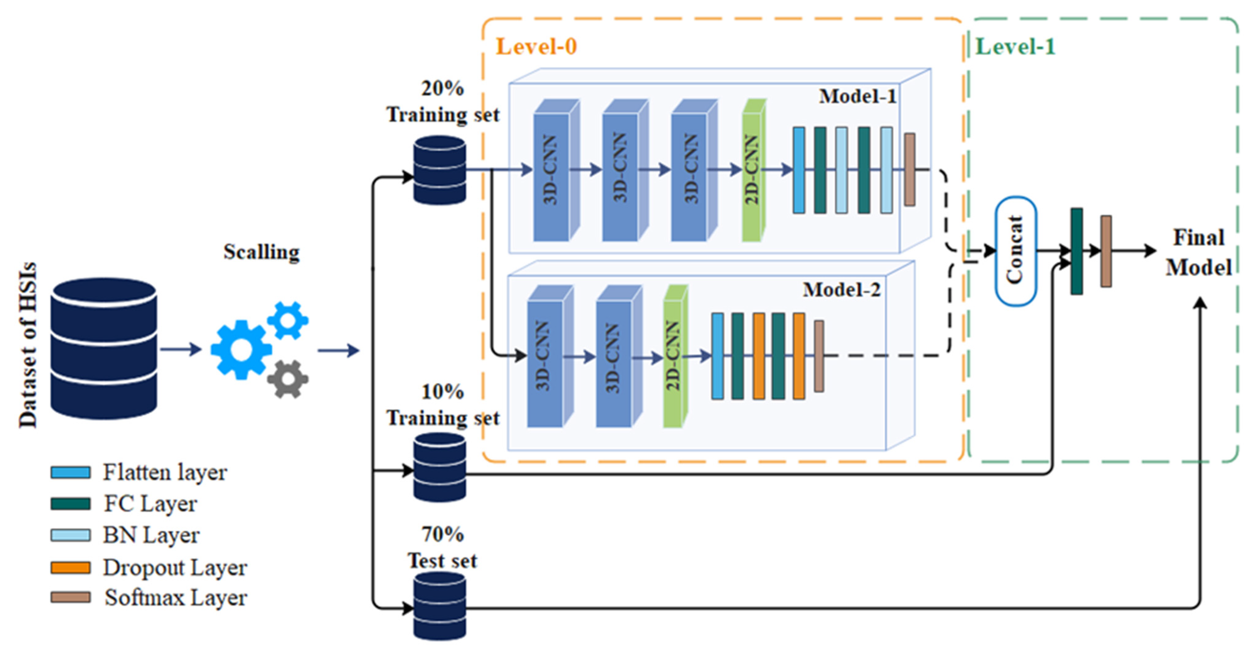
- To propose a novel framework that uses the meta-learner technique to train multi-class and multi-size datasets by concatenating and training the hybrid and multi-size kernel networks of CNN.
- To provide a new normalization method, called QPCA, based on the output of PCA and quantile transformation, which redistributes the data to be more normal and have less dimensionality.
- To present an efficient method that can extract more features from simple and complex spatial-spectral data simultaneously by combining the output of the shallow and deep networks without needing to increase the number of samples to increase the accuracy.
2. Methodology and Framework
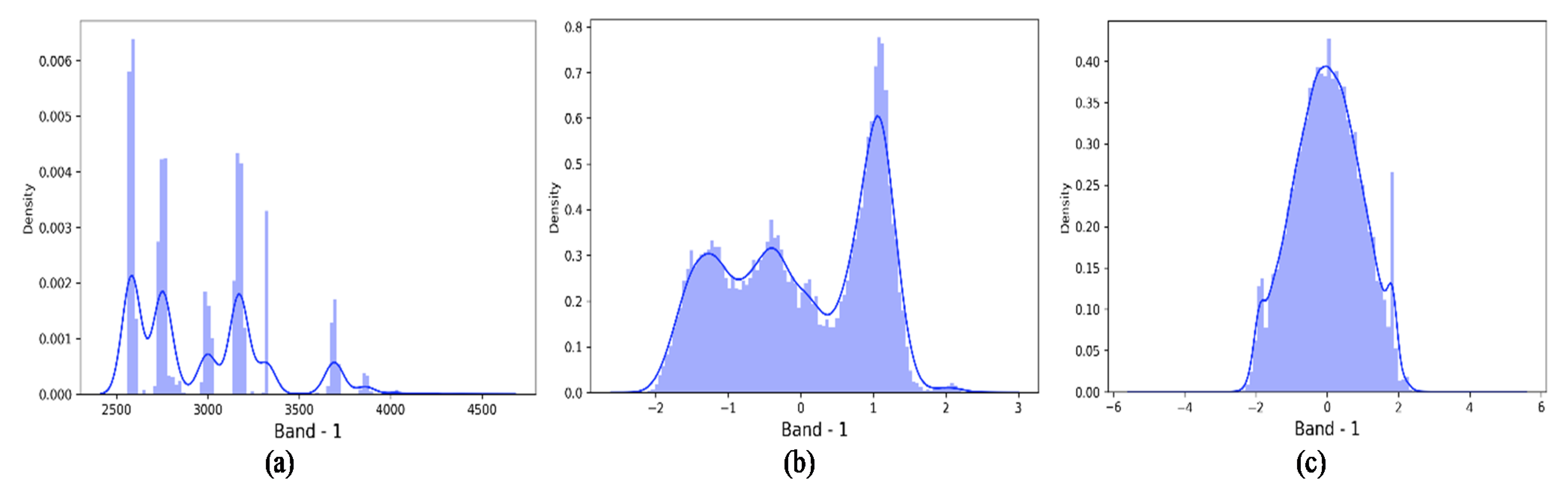
2.1. Optimize the Data Distribution (QPCA, Quantile Transformation Principal Components Analysis)
| Algorithm 1. The QPCA Processing. |
| Input: |
| Output: |
| 1: Standardize the d-dimensional of → . |
| 2: Getting the covariance matrix of |
| 3: Select the top k eigenvectors (𝑘 ≤ 𝑑) to build the weight matrix . |
| 4: Transform by multiplying it with the weight vector of 𝑘 to get |
| 5: Normalize the distribution of by quantile transformation: |
2.2. Framework
| Algorithm 2. The Steps of the Proposed MLHM. |
| Input: Training data and |
| Output: An ensemble classifier |
| 1: Step 1: Learn Level-0 classifiers |
| 2: for to do |
| 3: Learn a base classifier based on |
| 4: end for |
| 5: Step 2: Train the dataset of |
| 6: Keep the weights of training stage |
| 7: Step 3: Learn the Level-1 classifier |
| 8: for do |
| 9: Redistribute weights based on the new training data and the previous weights. Learn |
| a new classifier based on the newly constructed data set |
| 10: end for |
| 11: Return |
3. Experiment
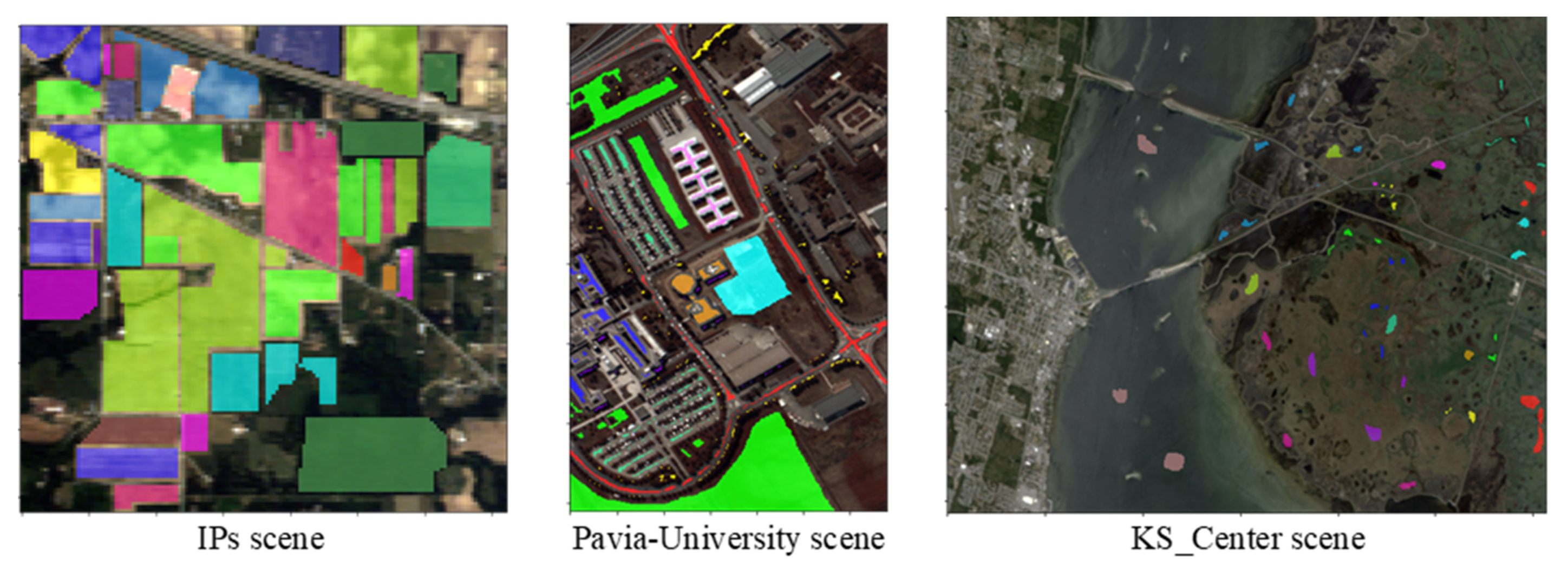
3.1. Datasets
3.2. Experimental Results and Comparisons
3.2.1. QPCA Output
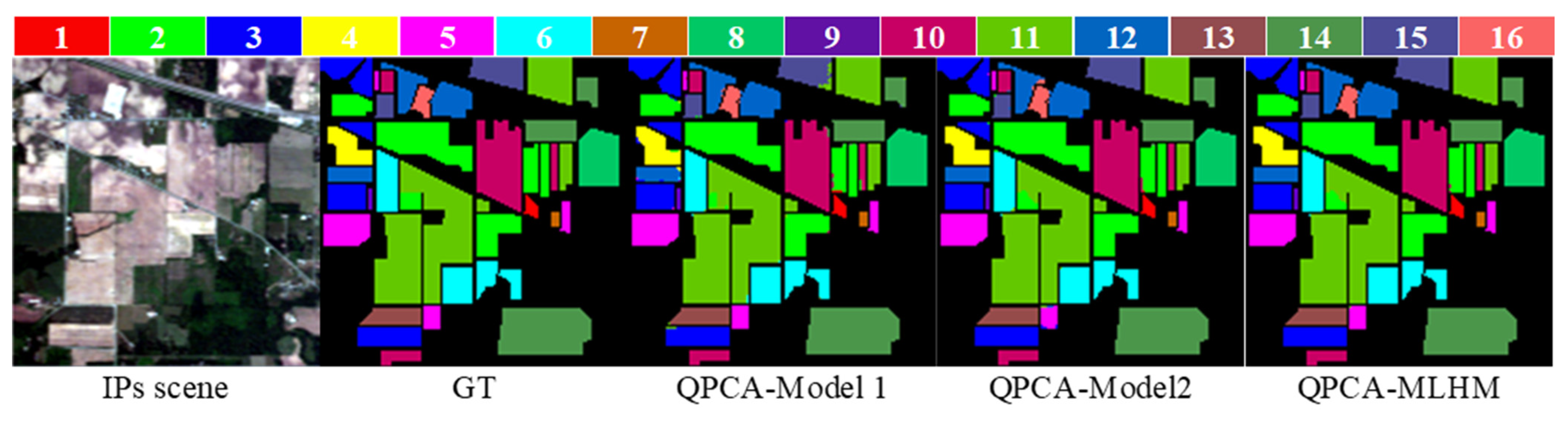
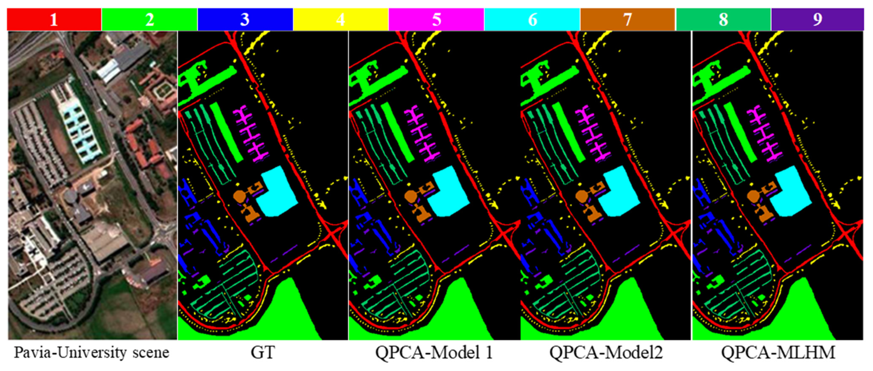
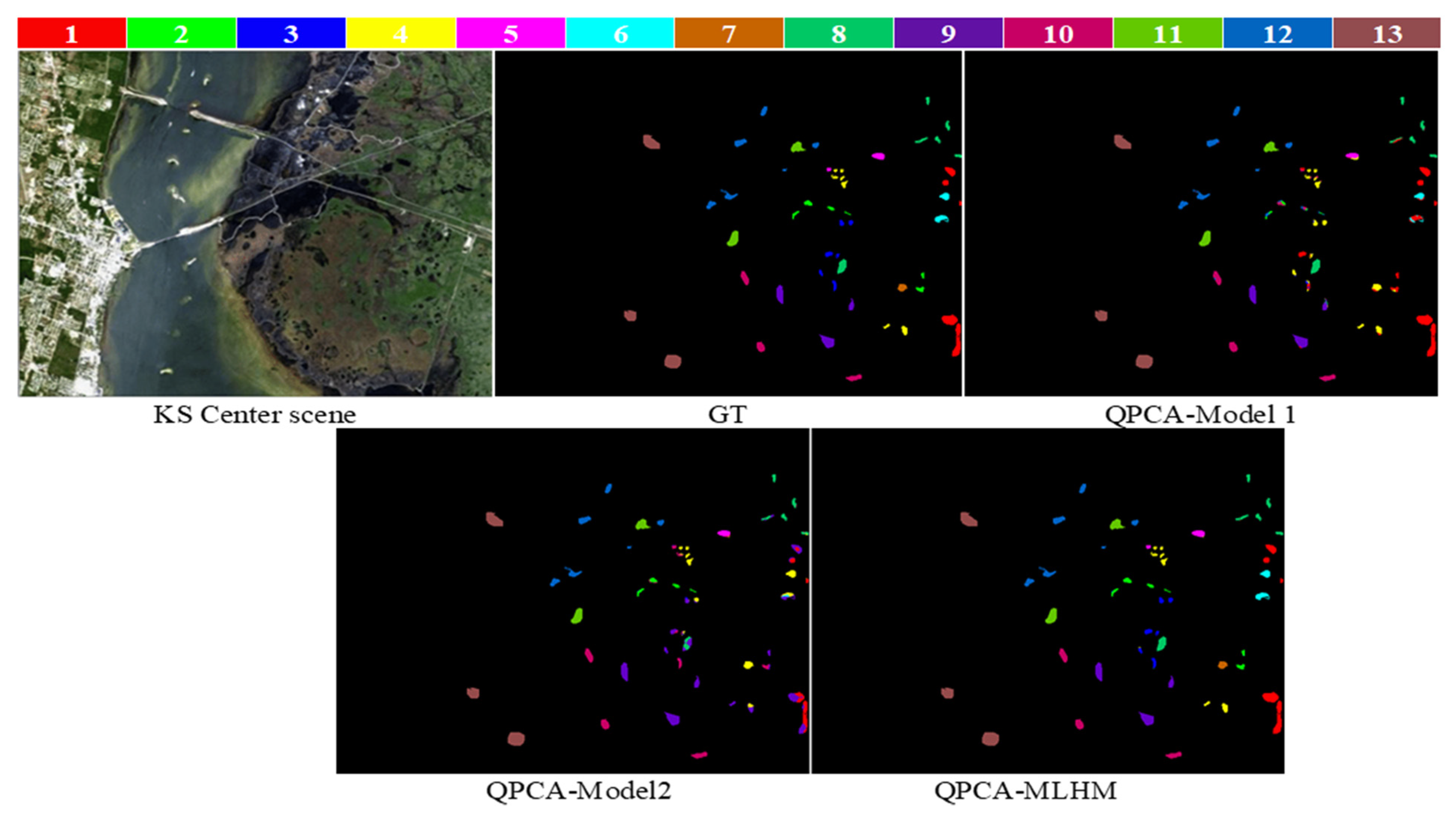
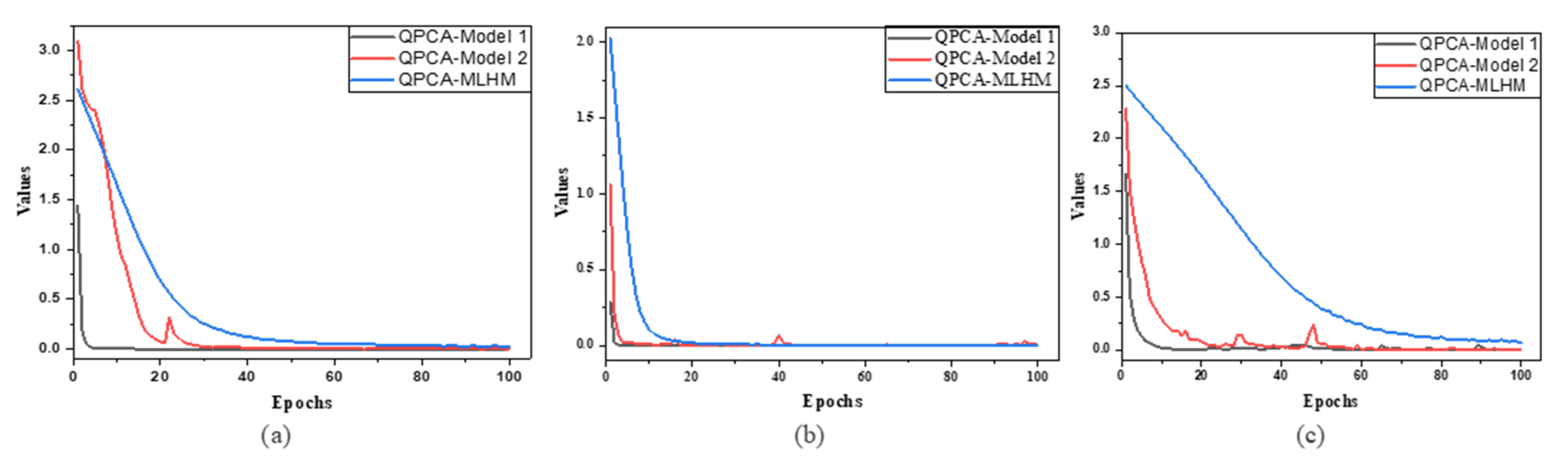
3.2.2. Meta-Learner Hybrid Model (MLHM) Results
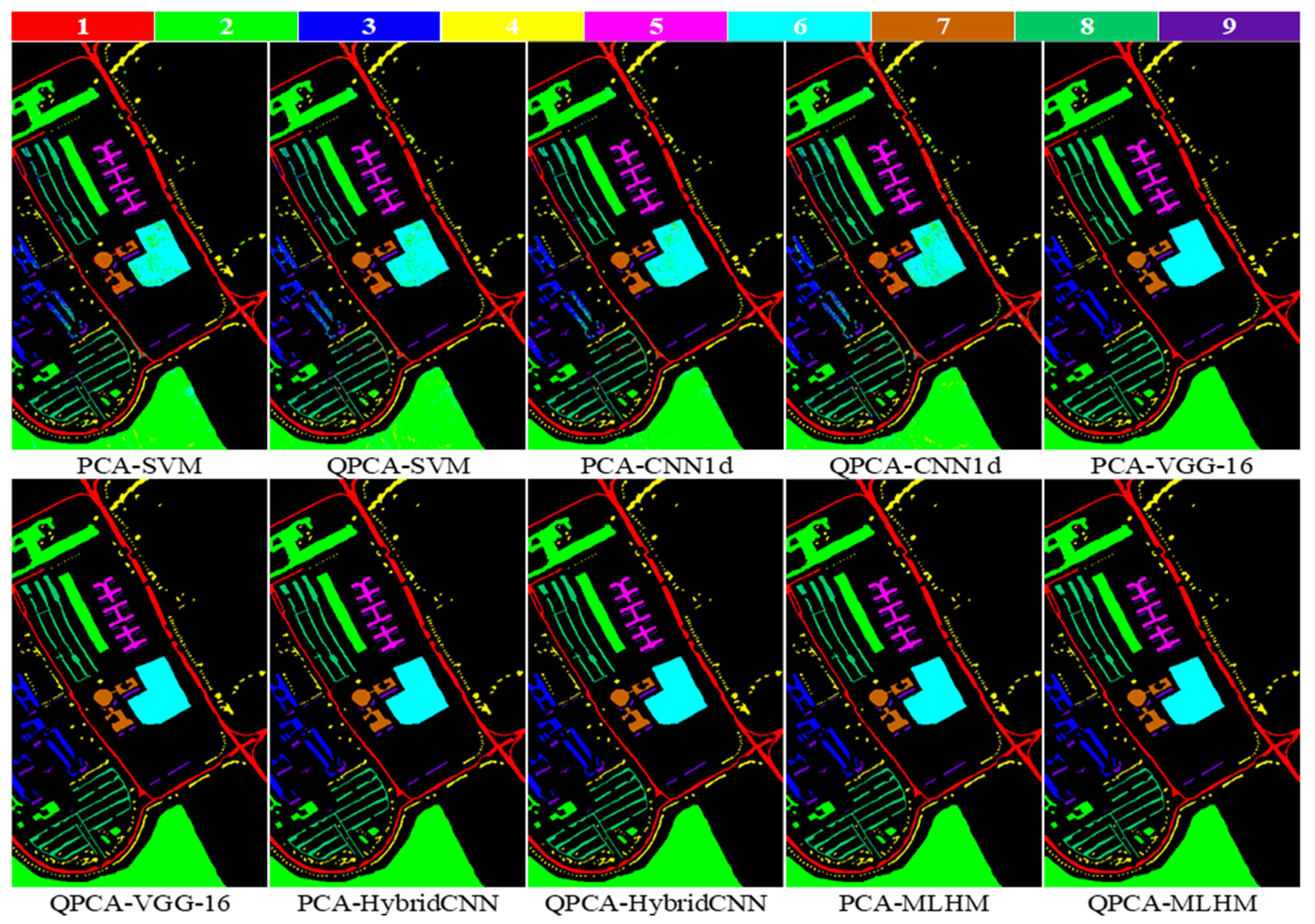
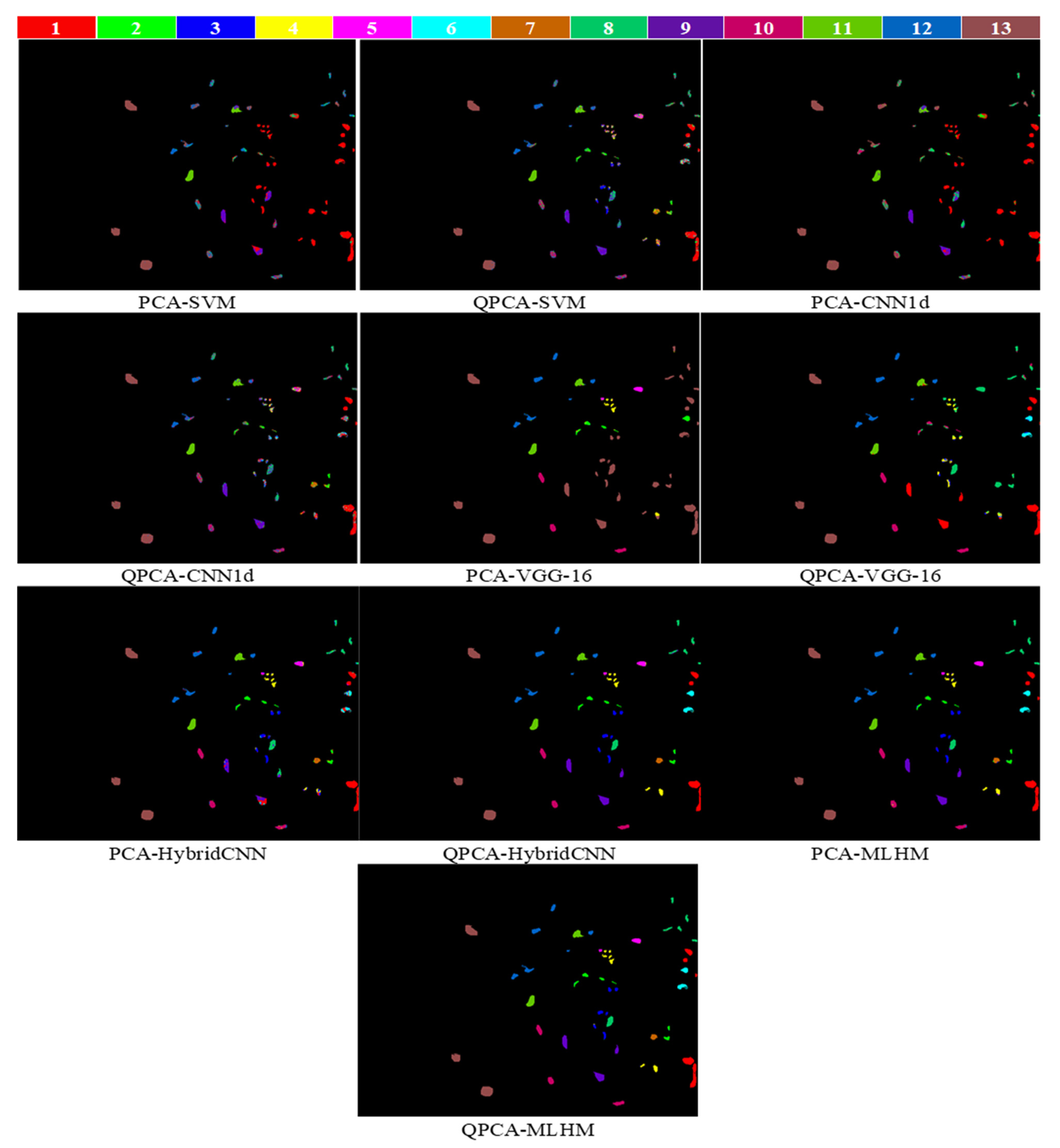
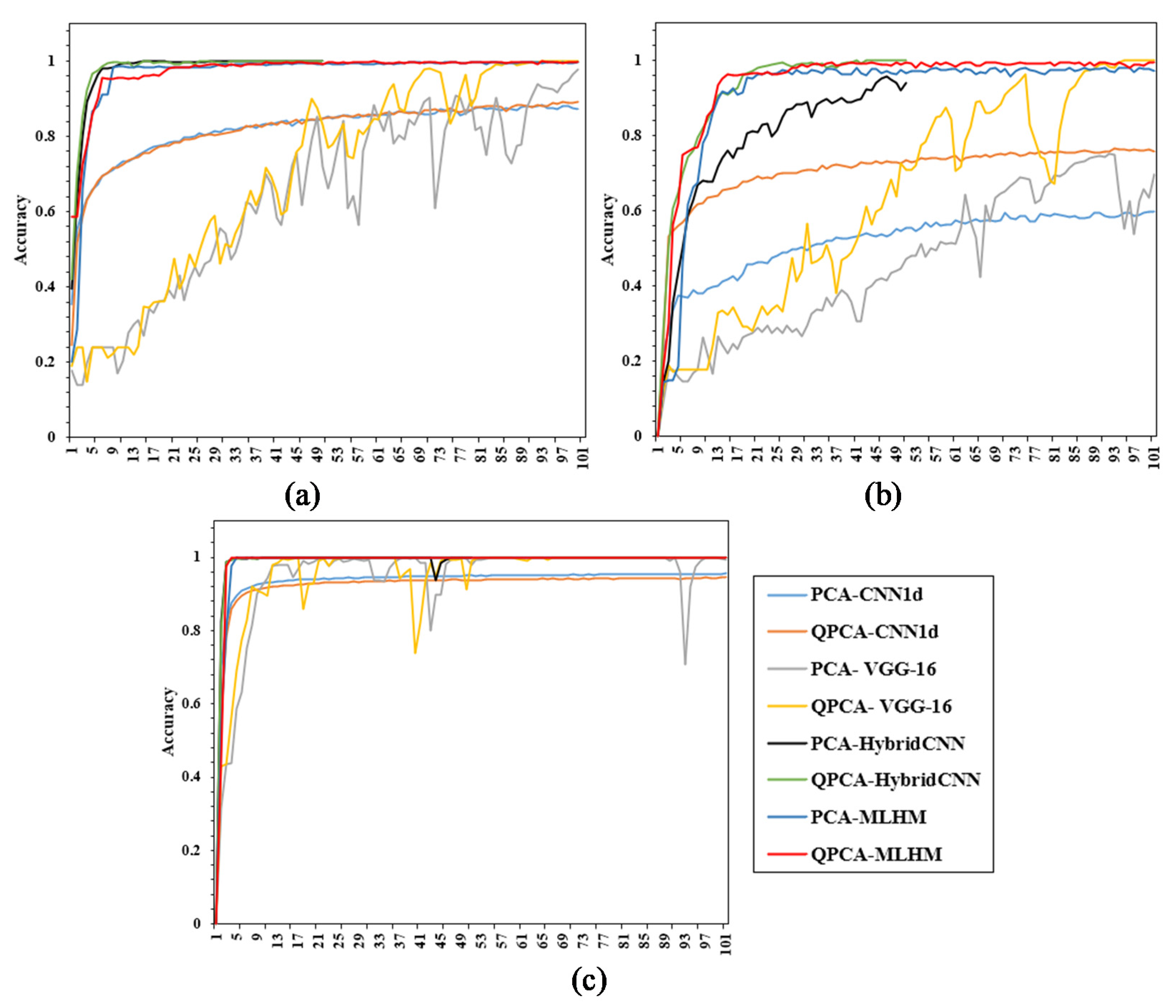
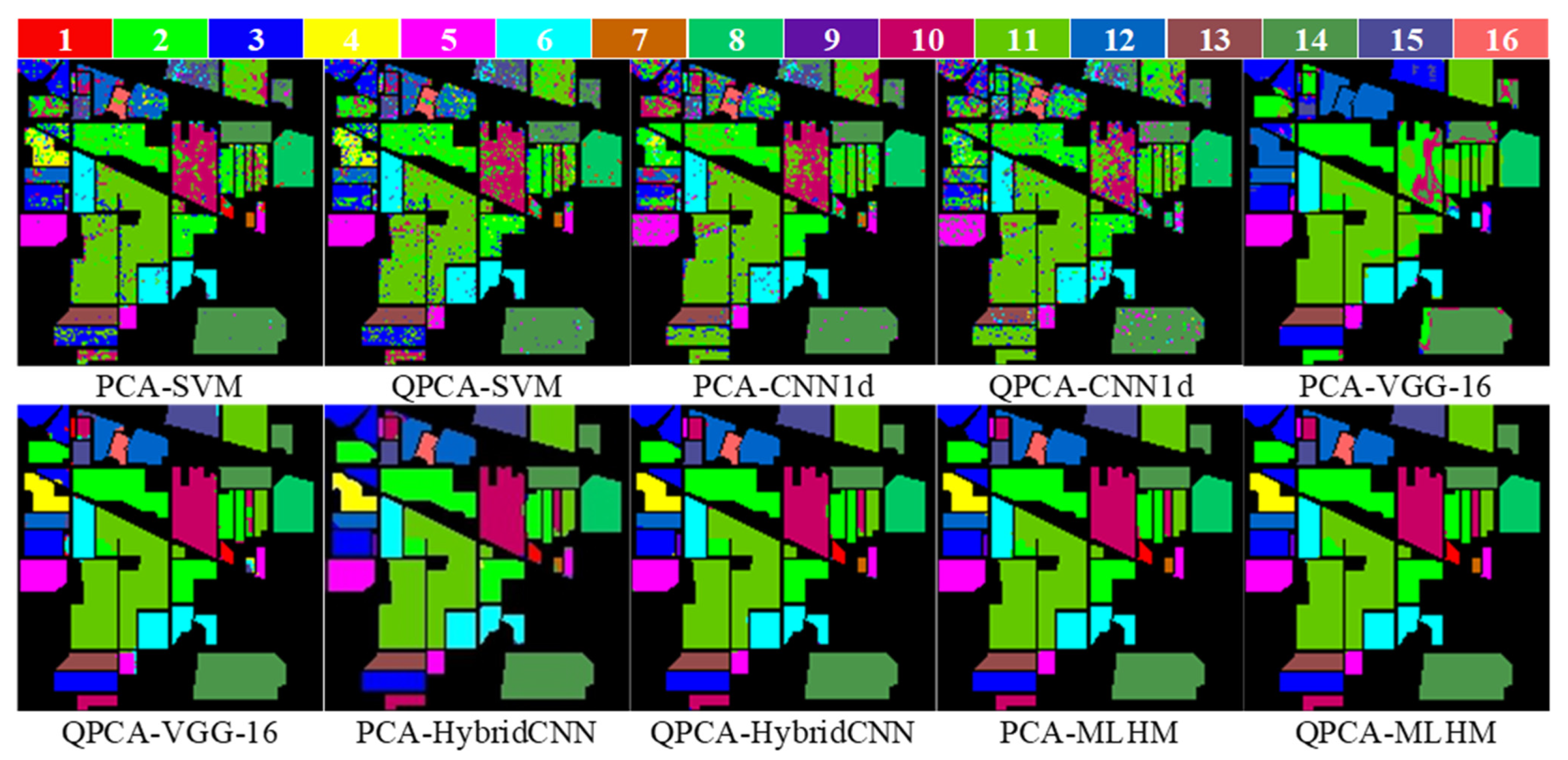
3.2.3. Comparisons with Other Methods
4. Conclusions
Author Contributions
Funding
Data Availability Statement
Conflicts of Interest
References
- Mei, X.; Pan, E.; Ma, Y.; Dai, X.; Huang, J.; Fan, F.; Du, Q.; Zheng, H.; Ma, J. Spectral-Spatial Attention Networks for Hyperspectral Image Classification. Remote Sens. 2019, 11, 963. [Google Scholar] [CrossRef] [Green Version]
- Tao, C.; Wang, Y.; Cui, W.; Zou, B.; Zou, Z.; Tu, Y. A transferable spectroscopic diagnosis model for predicting arsenic contamination in soil. Sci. Total Environ. 2019, 669, 964–972. [Google Scholar] [CrossRef]
- Ma, L.; Crawford, M.M.; Zhu, L.; Liu, Y. Centroid and Covariance Alignment-Based Domain Adaptation for Unsupervised Classification of Remote Sensing Images. IEEE Trans. Geosci. Remote Sens. 2018, 57, 2305–2323. [Google Scholar] [CrossRef]
- Luft, L.; Neumann, C.; Freude, M.; Blaum, N.; Jeltsch, F. Hyperspectral modeling of ecological indicators—A new approach for monitoring former military training areas. Ecol. Indic. 2014, 46, 264–285. [Google Scholar] [CrossRef]
- Camps-Valls, G.; Tuia, D.; Bruzzone, L.; Benediktsson, J.A. Advances in Hyperspectral Image Classification: Earth Monitoring with Statistical Learning Methods. IEEE Signal Process. Mag. 2013, 31, 45–54. [Google Scholar] [CrossRef] [Green Version]
- Tusa, E.; Laybros, A.; Monnet, J.-M.; Dalla Mura, M.; Barré, J.-B.; Vincent, G.; Dalponte, M.; Féret, J.-B.; Chanussot, J. Fusion of hyperspectral imaging and LiDAR for forest monitoring. In Hyperspectral Imaging; Amigo, J.M., Ed.; Elsevier: Amsterdam, The Netherlands, 2020; Volume 32, pp. 281–303. ISBN 0922-3487. [Google Scholar] [CrossRef]
- Guo, A.T.; Huang, W.J.; Dong, Y.Y.; Ye, H.C.; Ma, H.Q.; Liu, B.; Wu, W.B.; Ren, Y.; Ruan, C.; Geng, Y. Wheat Yellow Rust Detection Using UAV-Based Hyperspectral Technology. Remote Sens. 2021, 13, 123. [Google Scholar] [CrossRef]
- Zheng, Q.; Huang, W.; Ye, H.; Dong, Y.; Shi, Y.; Chen, S. Using continous wavelet analysis for monitoring wheat yellow rust in different infestation stages based on unmanned aerial vehicle hyperspectral images. Appl. Opt. 2020, 59, 8003. [Google Scholar] [CrossRef]
- Cui, J.; Yan, B.; Dong, X.; Zhang, S.; Zhang, J.; Tian, F.; Wang, R. Temperature and emissivity separation and mineral mapping based on airborne TASI hyperspectral thermal infrared data. Int. J. Appl. Earth Obs. Geoinf. 2015, 40, 19–28. [Google Scholar] [CrossRef]
- Li, Y.; Qian, M.; Liu, P.; Cai, Q.; Li, X.; Guo, J.; Yan, H.; Yu, F.; Yuan, K.; Yu, J.; et al. The recognition of rice images by UAV based on capsule network. Clust. Comput. 2018, 22, 9515–9524. [Google Scholar] [CrossRef]
- Zhang, Y.; Ma, Y.; Dai, X.; Li, H.; Mei, X.; Ma, J. Locality-constrained sparse representation for hyperspectral image classification. Inf. Sci. 2020, 546, 858–870. [Google Scholar] [CrossRef]
- McInnes, L.; Healy, J.; Melville, J. Umap: Uniform manifold approximation and projection for dimension reduction. arXiv 2018, arXiv:1802.03426. [Google Scholar]
- Anowar, F.; Sadaoui, S.; Selim, B. Conceptual and empirical comparison of dimensionality reduction algorithms (PCA, KPCA, LDA, MDS, SVD, LLE, ISOMAP, LE, ICA, t-SNE). Comput. Sci. Rev. 2021, 40, 100378. [Google Scholar] [CrossRef]
- Imani, M.; Ghassemian, H. An overview on spectral and spatial information fusion for hyperspectral image classification: Current trends and challenges. Inf. Fusion 2020, 59, 59–83. [Google Scholar] [CrossRef]
- Ghojogh, B.; Samad, M.N.; Mashhadi, S.A.; Kapoor, T.; Ali, W.; Karray, F.; Crowley, M. Feature Selection and Feature Extraction in Pattern Analysis: A Literature Review. arXiv 2019, arXiv:1905.02845. [Google Scholar]
- Zhang, X.; Wei, Y.; Yao, H.; Ye, Z.; Zhou, Y.; Zhao, Y. Locally Homogeneous Covariance Matrix Representation for Hyperspectral Image Classification. IEEE J. Sel. Top. Appl. Earth Obs. Remote Sens. 2021, 14, 9396–9407. [Google Scholar] [CrossRef]
- Yao, H.; Yang, M.; Chen, T.; Wei, Y.; Zhang, Y. Depth-based human activity recognition via multi-level fused features and fast broad learning system. Int. J. Distrib. Sens. Netw. 2020, 16, 1550147720907830. [Google Scholar] [CrossRef] [Green Version]
- Yuan, Y.; Jin, M. Multi-type spectral spatial feature for hyperspectral image classification. Neurocomputing 2021, in press. [Google Scholar] [CrossRef]
- Mohan, A.; Venkatesan, M. HybridCNN based hyperspectral image classification using multiscale spatiospectral features. Infrared Phys. Technol. 2020, 108, 103326. [Google Scholar] [CrossRef]
- Roy, S.K.; Dubey, S.R.; Chatterjee, S.; Chaudhuri, B.B. FuSENet: Fused squeeze-and-excitation network for spectral-spatial hyperspectral image classification. IET Image Process. 2020, 14, 1653–1661. [Google Scholar] [CrossRef]
- Roy, S.K.; Krishna, G.; Dubey, S.R.; Chaudhuri, B.B. HybridSN: Exploring 3-D–2-D CNN Feature Hierarchy for Hyperspectral Image Classification. IEEE Geosci. Remote Sens. Lett. 2019, 17, 277–281. [Google Scholar] [CrossRef] [Green Version]
- Li, S.; Song, W.; Fang, L.; Chen, Y.; Ghamisi, P.; Benediktsson, J.A. Deep Learning for Hyperspectral Image Classification: An Overview. IEEE Trans. Geosci. Remote Sens. 2019, 57, 6690–6709. [Google Scholar] [CrossRef] [Green Version]
- Camps-Valls, G.; Bruzzone, L. Kernel-based methods for hyperspectral image classification. IEEE Trans. Geosci. Remote Sens. 2005, 43, 1351–1362. [Google Scholar] [CrossRef]
- Chen, Y.; Nasrabadi, N.M.; Tran, T.D. Hyperspectral Image Classification Using Dictionary-Based Sparse Representation. IEEE Trans. Geosci. Remote Sens. 2011, 49, 3973–3985. [Google Scholar] [CrossRef]
- Li, S.; Wu, H.; Wan, D.; Zhu, J. An effective feature selection method for hyperspectral image classification based on genetic algorithm and support vector machine. Knowl.-Based Syst. 2011, 24, 40–48. [Google Scholar] [CrossRef]
- Yang, L.; Yang, S.; Jin, P.; Zhang, R. Semi-Supervised Hyperspectral Image Classification Using Spatio-Spectral Laplacian Support Vector Machine. IEEE Geosci. Remote Sens. Lett. 2014, 11, 651–655. [Google Scholar] [CrossRef]
- Chen, Y.-N.; Thaipisutikul, T.; Han, C.-C.; Liu, T.-J.; Fan, K.-C. Feature Line Embedding Based on Support Vector Machine for Hyperspectral Image Classification. Remote Sens. 2021, 13, 130. [Google Scholar] [CrossRef]
- Guo, Y.; Han, S.; Li, Y.; Zhang, C.; Bai, Y. K-Nearest Neighbor combined with guided filter for hyperspectral image classification. Procedia Comput. Sci. 2018, 129, 159–165. [Google Scholar] [CrossRef]
- Tu, B.; Huang, S.; Fang, L.; Zhang, G.; Wang, J.; Zheng, B. Hyperspectral Image Classification via Weighted Joint Nearest Neighbor and Sparse Representation. IEEE J. Sel. Top. Appl. Earth Obs. Remote Sens. 2018, 11, 4063–4075. [Google Scholar] [CrossRef]
- Huang, K.; Li, S.; Kang, X.; Fang, L. Spectral–Spatial Hyperspectral Image Classification Based on KNN. Sens. Imaging 2016, 17, 1–13. [Google Scholar] [CrossRef]
- Cao, X.; Yao, J.; Xu, Z.; Meng, D. Hyperspectral Image Classification with Convolutional Neural Network and Active Learning. IEEE Trans. Geosci. Remote Sens. 2020, 58, 4604–4616. [Google Scholar] [CrossRef]
- Hang, R.; Li, Z.; Liu, Q.; Ghamisi, P.; Bhattacharyya, S.S. Hyperspectral Image Classification with Attention-Aided CNNs. IEEE Trans. Geosci. Remote Sens. 2021, 59, 2281–2293. [Google Scholar] [CrossRef]
- Yu, C.; Han, R.; Song, M.; Liu, C.; Chang, C.-I. A Simplified 2D-3D CNN Architecture for Hyperspectral Image Classification Based on Spatial–Spectral Fusion. IEEE J. Sel. Top. Appl. Earth Obs. Remote Sens. 2020, 13, 2485–2501. [Google Scholar] [CrossRef]
- Bandyopadhyay, M. Multi-stack hybrid CNN with non-monotonic activation functions for hyperspectral satellite image classification. Neural Comput. Appl. 2021, 33, 14809–14822. [Google Scholar] [CrossRef]
- Huang, L.; Chen, Y. Dual-Path Siamese CNN for Hyperspectral Image Classification with Limited Training Samples. IEEE Geosci. Remote Sens. Lett. 2021, 18, 518–522. [Google Scholar] [CrossRef]
- Zhao, Q.; Jia, S.; Li, Y. Hyperspectral remote sensing image classification based on tighter random projection with minimal intra-class variance algorithm. Pattern Recognit. 2021, 111, 107635. [Google Scholar] [CrossRef]
- Ramamurthy, M.; Robinson, Y.H.; Vimal, S.; Suresh, A. Auto encoder based dimensionality reduction and classification using convolutional neural networks for hyperspectral images. Microprocess. Microsyst. 2020, 79, 103280. [Google Scholar] [CrossRef]
- Paul, A.; Bhoumik, S.; Chaki, N. SSNET: An improved deep hybrid network for hyperspectral image classification. Neural Comput. Appl. 2020, 33, 1575–1585. [Google Scholar] [CrossRef]
- Wei, Y.; Zhou, Y. Spatial-Aware Network for Hyperspectral Image Classification. Remote Sens. 2021, 13, 3232. [Google Scholar] [CrossRef]
- Zhao, J.; Huang, T.; Zhou, Z. Hyperspectral image super-resolution using recursive densely convolutional neural network with spatial constraint strategy. Neural Comput. Appl. 2020, 32, 14471–14481. [Google Scholar] [CrossRef]
- Zhao, G.; Liu, G.; Fang, L.; Tu, B.; Ghamisi, P. Multiple convolutional layers fusion framework for hyperspectral image classification. Neurocomputing 2019, 339, 149–160. [Google Scholar] [CrossRef]
- Al-Alimi, D.; Shao, Y.; Feng, R.; Al-Qaness, M.A.A.; Elaziz, M.A.; Kim, S. Multi-Scale Geospatial Object Detection Based on Shallow-Deep Feature Extraction. Remote Sens. 2019, 11, 2525. [Google Scholar] [CrossRef] [Green Version]
- Cao, F.; Guo, W. Cascaded dual-scale crossover network for hyperspectral image classification. Knowl.-Based Syst. 2019, 189, 105122. [Google Scholar] [CrossRef]
- Yang, J.; Xiong, W.; Li, S.; Xu, C. Learning structured and non-redundant representations with deep neural networks. Pattern Recognit. 2018, 86, 224–235. [Google Scholar] [CrossRef]
- Guo, Y.; Cao, H.; Bai, J.; Bai, Y. High Efficient Deep Feature Extraction and Classification of Spectral-Spatial Hyperspectral Image Using Cross Domain Convolutional Neural Networks. IEEE J. Sel. Top. Appl. Earth Obs. Remote Sens. 2019, 12, 1–12. [Google Scholar] [CrossRef]
- Hu, J.; Shen, L.; Sun, G. Squeeze-and-Excitation Networks. In Proceedings of the IEEE Conference on Computer Vision and Pattern Recognition (CVPR), Salt Lake City, UT, USA, 18–23 June 2018; pp. 7132–7141. [Google Scholar]
- Lin, T.-Y.; Dollár, P.; Girshick, R.; He, K.; Hariharan, B.; Belongie, S. Feature pyramid networks for object detection. In Proceedings of the IEEE Conference on Computer Vision and Pattern Recognition, Honolulu, HI, USA, 21–26 July 2017; pp. 2117–2125. [Google Scholar]
- Gao, H.; Yang, Y.; Li, C.; Zhang, X.; Zhao, J.; Yao, D. Convolutional neural network for spectral-spatial classification of hyperspectral images. Neural Comput. Appl. 2019, 31, 8997–9012. [Google Scholar] [CrossRef]
- Ribeiro, M.H.D.M.; Coelho, L.D.S. Ensemble approach based on bagging, boosting and stacking for short-term prediction in agribusiness time series. Appl. Soft Comput. 2019, 86, 105837. [Google Scholar] [CrossRef]
- Shamaei, E.; Kaedi, M. Suspended sediment concentration estimation by stacking the genetic programming and neuro-fuzzy predictions. Appl. Soft Comput. 2016, 45, 187–196. [Google Scholar] [CrossRef]
- Pernía-Espinoza, A.; Fernandez-Ceniceros, J.; Antonanzas, J.; Urraca, R.; Martinez-De-Pison, F. Stacking ensemble with parsimonious base models to improve generalization capability in the characterization of steel bolted components. Appl. Soft Comput. 2018, 70, 737–750. [Google Scholar] [CrossRef]
- Wozniak, M.; Graña, M.; Corchado, E. A survey of multiple classifier systems as hybrid systems. Inf. Fusion 2014, 16, 3–17. [Google Scholar] [CrossRef] [Green Version]
- Kang, S.; Cho, S.; Kang, P. Multi-class classification via heterogeneous ensemble of one-class classifiers. Eng. Appl. Artif. Intell. 2015, 43, 35–43. [Google Scholar] [CrossRef]
- Taormina, V.; Cascio, D.; Abbene, L.; Raso, G. Performance of Fine-Tuning Convolutional Neural Networks for HEp-2 Image Classification. Appl. Sci. 2020, 10, 6940. [Google Scholar] [CrossRef]
- Zhong, C.; Zhang, J.; Wu, S.; Zhang, Y. Cross-Scene Deep Transfer Learning with Spectral Feature Adaptation for Hyperspectral Image Classification. IEEE J. Sel. Top. Appl. Earth Obs. Remote Sens. 2020, 13, 2861–2873. [Google Scholar] [CrossRef]
- Liu, X.; Yu, L.; Peng, P.; Lu, F. A Stacked Generalization Framework for City Traffic Related Geospatial Data Analysis. In Web Technologies and Applications; Morishima, A., Zhang, R., Zhang, W., Chang, L., Fu, T.Z.J., Liu, K., Yang, X., Zhu, J., Zhang, Z., Eds.; Springer International Publishing: Cham, Switzerland, 2016; pp. 265–276. [Google Scholar]
- Garcia-Ceja, E.; Galván-Tejada, C.E.; Brena, R. Multi-view stacking for activity recognition with sound and accelerometer data. Inf. Fusion 2018, 40, 45–56. [Google Scholar] [CrossRef]
- Xu, Y.; Du, B.; Zhang, F.; Zhang, L. Hyperspectral image classification via a random patches network. ISPRS J. Photogramm. Remote Sens. 2018, 142, 344–357. [Google Scholar] [CrossRef]
- Cheng, C.; Li, H.; Peng, J.; Cui, W.; Zhang, L. Hyperspectral Image Classification Via Spectral-Spatial Random Patches Network. IEEE J. Sel. Top. Appl. Earth Obs. Remote Sens. 2021, 14, 4753–4764. [Google Scholar] [CrossRef]
- Garbin, C.; Zhu, X.; Marques, O. Dropout vs. batch normalization: An empirical study of their impact to deep learning. Multimed. Tools Appl. 2020, 79, 12777–12815. [Google Scholar] [CrossRef]
- Fernández, A.; García, S.; Galar, M.; Prati, R.C.; Krawczyk, B.; Herrera, F. Learning from Imbalanced Data Sets, 1st ed.; Springer International Publishing: Cham, Switzerland, 2018; ISBN 978-3-319-98073-7. [Google Scholar] [CrossRef]
- Paoletti, M.E.; Haut, J.M.; Plaza, J.; Plaza, A. Deep learning classifiers for hyperspectral imaging: A review. ISPRS J. Photogramm. Remote Sens. 2019, 158, 279–317. [Google Scholar] [CrossRef]
- Jiao, L.; Liang, M.; Chen, H.; Yang, S.; Liu, H.; Cao, X. Deep Fully Convolutional Network-Based Spatial Distribution Prediction for Hyperspectral Image Classification. IEEE Trans. Geosci. Remote Sens. 2017, 55, 5585–5599. [Google Scholar] [CrossRef]
- Chu, Y.; Lin, H.; Yang, L.; Zhang, D.; Diao, Y.; Fan, X.; Shen, C. Hyperspectral image classification based on discriminative locality preserving broad learning system. Knowl.-Based Syst. 2020, 206, 106319. [Google Scholar] [CrossRef]


| Level-0 | Level-1 | |
|---|---|---|
| Model-1 | Model-2 | |
| 3D-Convolutional Neural Networks (CNN) 8—(3, 3, 7)—ReLu * | 3D-CNN 8—(3, 3, 7)—ReLu | -- |
| 3D-CNN 16—(3, 3, 5)—ReLu | 3D-CNN 16—(3, 3, 5)—ReLu | -- |
| 3D-CNN 32—(3, 3, 3)—ReLu | -- | -- |
| 2D-CNN 64—(3, 3)—ReLu | 2D-CNN 64—(3, 3)—ReLu | |
| Flatten | Flatten | -- |
| FC 256—ReLu ** | FC 256—ReLu | Conct |
| BN | Dropout | -- |
| FC 128—ReLu | FC 128—ReLu | FC 128—ReLu |
| BN | BN | -- |
| SoftMax | SoftMax | SoftMax |
| Normal | PCA | QPCA | ||||
|---|---|---|---|---|---|---|
| Count | 21,025 | 21,025 | 21,025 |  | 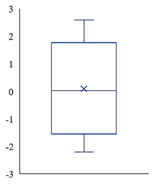 | 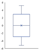 |
| Mean | 2957.36 | 6.5 × 10⁻¹⁶ | −0.0011 | |||
| Std | 354.919 | 1 | 0.95359 | |||
| Min | 2560 | −2.2061 | −5.1993 | |||
| 25% | 2602 | −0.887 | −0.6739 | |||
| 50% | 2780 | 0.0208 | 0.0031 | |||
| 75% | 3179 | 0.97266 | 0.67668 | |||
| Max | 4536 | 2.58808 | 5.19934 | (a) | (b) | (c) |
| # | Classes | Level-0 Samples | Level-1 Samples | Testing Samples | Level-0 | Level-1 | |
|---|---|---|---|---|---|---|---|
| QPCA-Model-1 | QPCA-Model-2 | QPCA-MLHM | |||||
| 1 | Alfalfa | 9 | 4 | 33 | 1 | 1 | 1 |
| 2 | Corn-notill (CN) | 285 | 114 | 1029 | 0.964 | 0.977 | 0.983 |
| 3 | Corn-mintill (CM) | 166 | 66 | 598 | 0.998 | 1 | 1 |
| 4 | Corn | 47 | 19 | 171 | 0.988 | 1 | 1 |
| 5 | Grass-pasture (GP) | 97 | 39 | 347 | 0.994 | 1 | 0.997 |
| 6 | Grass-trees (GT) | 146 | 58 | 526 | 0.998 | 0.990 | 0.994 |
| 7 | Grass-pasture-mowed (GPM) | 6 | 2 | 20 | 1 | 1 | 1 |
| 8 | Hay-windrowed (HW) | 96 | 38 | 344 | 1 | 1 | 1 |
| 9 | Oats | 4 | 2 | 14 | 1 | 1 | 1 |
| 10 | Soybean-notill (SN) | 194 | 78 | 700 | 0.994 | 1 | 1 |
| 11 | Soybean-mintill (SM) | 491 | 197 | 1767 | 0.998 | 0.998 | 0.997 |
| 12 | Soybean-clean (SC) | 118 | 48 | 427 | 0.991 | 0.979 | 0.998 |
| 13 | Wheat | 41 | 16 | 148 | 0.993 | 1 | 1 |
| 14 | Woods | 253 | 101 | 911 | 1 | 1 | 1 |
| 15 | Buildings-Grass-Trees-Drives (BGTD) | 77 | 31 | 278 | 1 | 0.996 | 1 |
| 16 | Stone-Steel-Towers (SST) | 19 | 7 | 67 | 0.970 | 0.970 | 0.970 |
| Kappa accuracy (%) | 99.119 | 99.320 | 99.536 | ||||
| Overall accuracy (%) | 99.228 | 99.404 | 99.594 | ||||
| Average accuracy (%) | 99.310 | 99.443 | 99.618 | ||||
| Training Time (s) | 138.50 | 70.02 | 28.28 | ||||
| Testing Time (s) | 1.61 | 1.22 | 2.66 | ||||
| # | Classes | Level-0 Samples | Level-1 Samples | Testing Samples | Level-0 | Level-1 | |
|---|---|---|---|---|---|---|---|
| QPCA-Model-1 | QPCA-Model-2 | QPCA-MLHM | |||||
| 1 | Asphalt | 1326 | 530 | 4775 | 1 | 1 | 1 |
| 2 | Meadows | 3730 | 1492 | 13427 | 1 | 1 | 1 |
| 3 | Gravel | 420 | 168 | 1511 | 0.999 | 1 | 1 |
| 4 | Trees | 613 | 245 | 2206 | 0.995 | 0.995 | 0.999 |
| 5 | Painted metal sheets (BMS) | 269 | 108 | 968 | 1 | 1 | 1 |
| 6 | Bare Soil (BS) | 1006 | 402 | 3621 | 1 | 1 | 1 |
| 7 | Bitumen | 266 | 106 | 958 | 1 | 0.994 | 1 |
| 8 | Self-Blocking Bricks (SBB) | 736 | 295 | 2651 | 0.999 | 0.995 | 0.999 |
| 9 | Shadows | 189 | 76 | 682 | 1 | 1 | 1 |
| Kappa accuracy (%) | 99.931 | 99.880 | 99.978 | ||||
| Overall accuracy (%) | 99.948 | 99.909 | 99.984 | ||||
| Average accuracy (%) | 99.920 | 99.83 | 99.977 | ||||
| Training Time (s) | 117.32 | 79.65 | 27.00 | ||||
| Testing Time (s) | 2.40 | 2.33 | 3.92 | ||||
| # | Classes | Level-0 Samples | Level-1 Samples | Testing Samples | Level-0 | Level-1 | |
|---|---|---|---|---|---|---|---|
| QPCA-Model-1 | QPCA-Model-2 | QPCA-MLHM | |||||
| 1 | Scrub | 152 | 61 | 548 | 1 | 1 | 1 |
| 2 | Willow swamp (WS) | 49 | 19 | 175 | 0.817 | 0.977 | 0.971 |
| 3 | Cabbage palm hammock (CPH) | 51 | 21 | 184 | 0.152 | 0.984 | 0.989 |
| 4 | Cabbage palm/oak hammock (CPOH) | 50 | 20 | 182 | 0.967 | 0.995 | 0.995 |
| 5 | Slash pine (SP) | 32 | 13 | 116 | 0.793 | 0.991 | 0.991 |
| 6 | Oak/broadleaf hammock (OBH) | 46 | 18 | 165 | 1 | 1 | 1 |
| 7 | Hardwood swamp (HS) | 21 | 8 | 76 | 1 | 1 | 1 |
| 8 | Graminoid marsh (GM) | 86 | 34 | 311 | 0.936 | 1 | 0.997 |
| 9 | Spartina marsh (SM) | 104 | 42 | 374 | 1 | 1 | 1 |
| 10 | Cattail marsh (CM) | 81 | 32 | 291 | 0.990 | 1 | 1 |
| 11 | Salt marsh (SM) | 84 | 34 | 301 | 1 | 1 | 1 |
| 12 | Mud flats (MF) | 101 | 40 | 362 | 0.994 | 1 | 1 |
| 13 | Wate | 185 | 74 | 668 | 1 | 1 | 1 |
| Kappa accuracy (%) | 92.774 | 99.733 | 99.703 | ||||
| Overall accuracy (%) | 93.525 | 99.760 | 99.734 | ||||
| Average accuracy (%) | 89.610 | 99.590 | 99.563 | ||||
| Training Time (s) | 86.13 | 15.28 | 6.04 | ||||
| Testing Time (s) | 0.35 | 0.31 | 0.51 | ||||
| # | Calsses | PCA-SVM | QPCA-SVM | PCA-CNN1d | QPCA-CNN1d | PCA-VGG-16 | QPCA-VGG-16 | PCA-Hybrid CNN | QPCA-Hybrid CNN | PCA-MLHM | QPCA-MLHM |
|---|---|---|---|---|---|---|---|---|---|---|---|
| 1 | Alfalfa | 0.70 | 0.16 | 0.78 | 0.44 | 0.00 | 0.00 | 0.97 | 0.97 | 1 | 1 |
| 2 | CN | 0.72 | 0.72 | 0.79 | 0.72 | 0.92 | 0.98 | 0.98 | 1 | 0.98 | 0.98 |
| 3 | CM | 0.75 | 0.67 | 0.71 | 0.70 | 0.94 | 0.99 | 0.99 | 1 | 1 | 1 |
| 4 | Corn | 0.64 | 0.45 | 0.62 | 0.60 | 1.00 | 0.93 | 0.98 | 1 | 1 | 1 |
| 5 | GP | 0.92 | 0.87 | 0.91 | 0.94 | 0.66 | 0.86 | 0.98 | 0.98 | 0.99 | 1 |
| 6 | GT | 0.95 | 0.96 | 0.93 | 0.95 | 0.57 | 0.99 | 1.00 | 1 | 1 | 0.99 |
| 7 | GPM | 0.96 | 0.82 | 1.00 | 1.00 | 0.00 | 0.00 | 1.00 | 1 | 1 | 1 |
| 8 | HW | 0.97 | 0.96 | 1.00 | 1.00 | 0.14 | 1.00 | 1.00 | 1 | 1 | 1 |
| 9 | Oats | 0.56 | 0.38 | 0.25 | 0.50 | 0.00 | 0.38 | 0.86 | 1 | 0.86 | 1 |
| 10 | SN | 0.72 | 0.65 | 0.73 | 0.70 | 0.93 | 0.95 | 0.98 | 0.98 | 1 | 1 |
| 11 | SM | 0.86 | 0.78 | 0.86 | 0.82 | 0.99 | 0.99 | 1.00 | 1 | 1 | 1 |
| 12 | SC | 0.74 | 0.64 | 0.69 | 0.69 | 0.95 | 0.98 | 0.97 | 0.99 | 0.98 | 1 |
| 13 | Wheat | 0.97 | 0.93 | 0.95 | 1.00 | 0.99 | 1.00 | 1.00 | 1 | 1 | 1 |
| 14 | Woods | 0.96 | 0.91 | 0.97 | 0.99 | 0.99 | 0.99 | 1.00 | 1 | 1 | 1 |
| 15 | BGTD | 0.61 | 0.57 | 0.69 | 0.60 | 0.96 | 0.84 | 0.99 | 1 | 1 | 1 |
| 16 | SST | 0.87 | 0.81 | 0.84 | 0.79 | 0.00 | 0.04 | 0.97 | 0.99 | 1 | 0.97 |
| KA (%) | 80 (0.09) | 73.91 (0.35) | 80.39 (1.27) | 78.33 (0.93) | 83.77 (13.13) | 94.68 (2.86) | 98.96 (0.82) | 99.25 (0.28) | 99.39 (0.07) | 99.41 (0.06) | |
| OA (%) | 82.50 (0.08) | 77.16 (0.31) | 82.84 (1.11) | 81.03 (0.80) | 85.87 (11.38) | 95.34 (2.50) | 99.09 (0.72) | 99.34 (0.25) | 99.47 (0.07) | 99.47 (0.06) | |
| AA (%) | 80.28 (0.18) | 70.63 (0.54) | 79.48 (3.15) | 78.24 (2.16) | 66.58 (19.31) | 81.89 (9.03) | 98.17 (1.04) | 98.71 (0.51) | 99.01 (0.40) | 99.36 (0.27) | |
| Tr.T. 1 (s) | 0.41 | 0.67 | 21.87 | 36.04 | 53.44 | 50.95 | 65.60 | 60.40 | 41.67 | 25.47 | |
| Ta.T. 2 (s) | 2.40 | 2.45 | 0.25 | 0.27 | 2.20 | 2.24 | 1.93 | 1.83 | 4.53 | 3.64 |
| # | Calsses | PCA-SVM | QPCA-SVM | PCA-CNN1d | QPCA-CNN1d | PCA-VGG-16 | QPCA- VGG-16 | PCA-Hybrid CNN | QPCA-Hybrid CNN | PCA-MLHM | QPCA- MLHM |
|---|---|---|---|---|---|---|---|---|---|---|---|
| 1 | Asphalt | 0.95 | 0.94 | 0.95 | 0.90 | 1 | 1 | 1 | 1 | 1 | 1 |
| 2 | Meadows | 0.98 | 0.96 | 0.98 | 0.96 | 1 | 1 | 1 | 1 | 1 | 1 |
| 3 | Gravel | 0.80 | 0.74 | 0.80 | 0.72 | 1 | 1 | 1 | 1 | 1 | 1 |
| 4 | Trees | 0.94 | 0.90 | 0.94 | 0.86 | 0.99 | 0.99 | 1 | 1 | 1 | 1 |
| 5 | BMS | 1.00 | 1.00 | 0.99 | 0.99 | 1 | 1 | 1 | 1 | 1 | 1 |
| 6 | BS | 0.88 | 0.88 | 0.91 | 0.83 | 1 | 1 | 1 | 1 | 1 | 1 |
| 7 | Bitumen | 0.86 | 0.86 | 0.91 | 0.79 | 1 | 1 | 0.99 | 1 | 1 | 1 |
| 8 | SBB | 0.91 | 0.82 | 0.89 | 0.82 | 1 | 1 | 0.98 | 1 | 1 | 1 |
| 9 | Shadows | 1 | 1 | 1 | 0.99 | 0.96 | 0.98 | 1 | 1 | 0.99 | 1 |
| KA (%) | 92.09 (0.01) | 89.66 (0.03) | 93.69 (0.30) | 91.88 (0.46) | 99.68 (0.24) | 99.81 (0.05) | 99.86 (0.06) | 99.93 (0.04) | 99.93 (0.01) | 99.94 (0.02) | |
| OA (%) | 93.86 (0.62) | 92.22 (0.02) | 95.25 (0.22) | 93.89 (0.35) | 99.76 (0.18) | 99.86 (0.04) | 99.90 (0.05) | 99.95 (0.03) | 99.94 (0.01) | 99.96 (0.02) | |
| AA (%) | 92.37 (0.59) | 90.07 (0.02) | 93.70 (0.40) | 92.01 (0.49) | 99.48 (0.29) | 99.68 (0.07) | 99.82 (0.07) | 99.91 (0.05) | 99.88 (0.04) | 99.90 (0.04) | |
| Tr.T. (s) | 1.58 | 2.03 | 77.81 | 78.64 | 234.05 | 208.66 | 239.24 | 211.71 | 38.25 | 38.05 | |
| Ta.T.(s) | 6.34 | 7.01 | 0.66 | 0.71 | 7.45 | 7.39 | 7.88 | 7.51 | 6.08 | 6.03 |
| # | Calsses | PCA-SVM | QPCA-SVM | PCA-CNN1d | QPCA-CNN1d | PCA-VGG-16 | QPCA-VGG-16 | PCA-Hybrid CNN | QPCA-Hybrid CNN | PCA-MLHM | QPCA-MLHM |
|---|---|---|---|---|---|---|---|---|---|---|---|
| 1 | Scrub | 0.97 | 0.90 | 0.97 | 0.95 | 0.98 | 1 | 0.96 | 1 | 1 | 1 |
| 2 | WS | 0 | 0.71 | 0.78 | 0.78 | 0.59 | 0.62 | 0.92 | 0.98 | 0.96 | 0.99 |
| 3 | CPH | 0 | 0.68 | 0 | 0.71 | 0 | 0.92 | 0.80 | 0.97 | 0.98 | 0.99 |
| 4 | CPOH | 0 | 0.35 | 0.16 | 0.48 | 0.60 | 0.94 | 0.64 | 0.99 | 0.88 | 0.99 |
| 5 | SP | 0 | 0.46 | 0 | 0.28 | 0.95 | 0 | 0.84 | 0.95 | 0.94 | 0.98 |
| 6 | OBH | 0 | 0.32 | 0 | 0.30 | 0.10 | 1 | 0.43 | 0.99 | 0.99 | 1 |
| 7 | HS | 0 | 0.71 | 0 | 0.71 | 0 | 0 | 0.70 | 1 | 0.93 | 1 |
| 8 | GM | 0.18 | 0.55 | 0.36 | 0.58 | 0.02 | 0.96 | 0.79 | 0.98 | 0.96 | 1 |
| 9 | SM | 0.71 | 0.83 | 0.76 | 0.87 | 0.04 | 1 | 0.80 | 1 | 1 | 1 |
| 10 | CM | 0.02 | 0.55 | 0.04 | 0.49 | 0.84 | 1 | 0.94 | 0.99 | 0.95 | 1 |
| 11 | SM | 0.88 | 0.92 | 0.83 | 0.96 | 0.60 | 1 | 1 | 1 | 1 | 1 |
| 12 | MF | 0.52 | 0.69 | 0.65 | 0.76 | 0.97 | 0.95 | 0.97 | 1 | 1 | 1 |
| 13 | Wate | 1 | 0.98 | 0.98 | 0.95 | 0.97 | 1 | 1 | 1 | 1 | 1 |
| KA (%) | 45.36 (0.10) | 71.80 (0.39) | 54.07 (1.69) | 73.36 (0.79) | 54.32 (13.94) | 91.54 (5.01) | 85.97 (4.59) | 99.11 (0.15) | 97.44 (0.61) | 99.57 (0.13) | |
| OA (%) | 52.68 (0.08) | 74.71 (0.35) | 59.54 (1.55) | 76.08 (0.72) | 60.15 (11.51) | 92.41 (4.49) | 87.38 (4.19) | 99.20 (0.14) | 97.70 (0.55) | 99.62 (0.11) | |
| AA (%) | 32.87 (0.06) | 66.85 (0.54) | 42.73 (0.96) | 69.39 (1.60) | 53.93 (12.17) | 85.54 (8.59) | 84.63 (3.10) | 98.76 (0.27) | 96.42 (0.83) | 99.34 (0.20) | |
| Tr.T. (s) | 0.07 | 0.04 | 20.14 | 21.15 | 72.54 | 72.72 | 32.42 | 36.96 | 8.80 | 8.38 | |
| Ta.T.(s) | 0.31 | 0.20 | 0.25 | 0.17 | 1.07 | 0.99 | 0.96 | 1.06 | 0.91 | 0.89 |
Publisher’s Note: MDPI stays neutral with regard to jurisdictional claims in published maps and institutional affiliations. |
© 2022 by the authors. Licensee MDPI, Basel, Switzerland. This article is an open access article distributed under the terms and conditions of the Creative Commons Attribution (CC BY) license (https://creativecommons.org/licenses/by/4.0/).
Share and Cite
AL-Alimi, D.; Al-qaness, M.A.A.; Cai, Z.; Dahou, A.; Shao, Y.; Issaka, S. Meta-Learner Hybrid Models to Classify Hyperspectral Images. Remote Sens. 2022, 14, 1038. https://doi.org/10.3390/rs14041038
AL-Alimi D, Al-qaness MAA, Cai Z, Dahou A, Shao Y, Issaka S. Meta-Learner Hybrid Models to Classify Hyperspectral Images. Remote Sensing. 2022; 14(4):1038. https://doi.org/10.3390/rs14041038
Chicago/Turabian StyleAL-Alimi, Dalal, Mohammed A. A. Al-qaness, Zhihua Cai, Abdelghani Dahou, Yuxiang Shao, and Sakinatu Issaka. 2022. "Meta-Learner Hybrid Models to Classify Hyperspectral Images" Remote Sensing 14, no. 4: 1038. https://doi.org/10.3390/rs14041038
APA StyleAL-Alimi, D., Al-qaness, M. A. A., Cai, Z., Dahou, A., Shao, Y., & Issaka, S. (2022). Meta-Learner Hybrid Models to Classify Hyperspectral Images. Remote Sensing, 14(4), 1038. https://doi.org/10.3390/rs14041038