Article

Decision Fusion of Deep Learning and Shallow Learning for Marine Oil Spill Detection

1
College of Oceanography and Space Informatics, China University of Petroleum, Qingdao 266580, China
2
First Institute of Oceanography, Ministry of Natural Resources, Qingdao 266061, China
3
School of Electronics and Information Engineering, Harbin Institute of Technology, Harbin 150001, China
*
Author to whom correspondence should be addressed.
Remote Sens. 2022, 14(3), 666; https://doi.org/10.3390/rs14030666
Submission received: 5 November 2021 / Revised: 18 January 2022 / Accepted: 27 January 2022 / Published: 30 January 2022
(This article belongs to the Special Issue Deep Learning for Remote Sensing Data)

Abstract

:
Marine oil spills are an emergency of great harm and have become a hot topic in marine environmental monitoring research. Optical remote sensing is an important means to monitor marine oil spills. Clouds, weather, and light control the amount of available data, which often limit feature characterization using a single classifier and therefore difficult to accurate monitoring of marine oil spills. In this paper, we develop a decision fusion algorithm to integrate deep learning methods and shallow learning methods based on multi-scale features for improving oil spill detection accuracy in the case of limited samples. Based on the multi-scale features after wavelet transform, two deep learning methods and two classical shallow learning algorithms are used to extract oil slick information from hyperspectral oil spill images. The decision fusion algorithm based on fuzzy membership degree is introduced to fuse multi-source oil spill information. The research shows that oil spill detection accuracy using the decision fusion algorithm is higher than that of the single detection algorithms. It is worth noting that oil spill detection accuracy is affected by different scale features. The decision fusion algorithm under the first-level scale features can further improve the accuracy of oil spill detection. The overall classification accuracy of the proposed method is 91.93%, which is 2.03%, 2.15%, 1.32%, and 0.43% higher than that of SVM, DBN, 1D-CNN, and MRF-CNN algorithms, respectively.

1. Introduction

Marine oil spill accidents have occurred frequently in recent years, causing serious harm to the marine environment. The explosion of the Deepwater Horizon platform in 2010 [1] led to crude oil leakage for nearly three months. Total oil spill volume reached about 4.9 million barrels, and the polluted seawater area was at least 10,000 square kilometers. The accident had a devastating impact on the marine ecological environment and biological resources in the Gulf of Mexico, which was the most serious oil spill accident in the history of the United States. More than 7000 tons of crude oil leaked from the blowout accident of Penglai 19-3C platform in 2011 [2], polluting 6200 square kilometers of seawater, resulting in serious pollution damage to the marine ecological environment of the Bohai Sea. The cost of compensation for marine ecological loss caused by the oil spill accident reached 250 million dollars. The explosion of coastal oil pipeline in the Jiaozhou Bay in 2013 [3] resulted in 62 deaths and 136 injuries. The oil spill area on the sea surface was about 3000 square meters, and the direct economic loss was about 120 million dollars. In 2018, the “SANCHI” tanker sank after collision with the cargo ship outside the Yangtze River Estuary in the East China Sea [4]. About 136,000 tons of condensate oil loaded on the tanker leaked, polluting 100 square kilometers of sea area, which threatened the marine ecological environment in the East China Sea and caused serious air pollution. Damage to marine ecological environments caused by large-scale marine oil spills is difficult to repair even over long periods of time. Worldwide attention has therefore been paid to the problem of marine oil spills, which have been listed by the American Academy of Science as one of 32 scientific problems to be solved by 2030.
Affected by wind and waves, the oil film on the sea surface is dynamic. Rapid and effective monitoring of the location and range of the oil spill is very important for rapid response. Remote sensing technology is the main means of emergency monitoring of oil spill on the sea surface, and has the outstanding advantages of a large area, synchronous and rapid detection. Using remote sensing data can not only monitor oil spill on sea in a large area, guide marine surveillance ships and aircraft to carry out law enforcement monitoring, but also provide the basis for law enforcement claims. At the same time, the range of oil pollution and the direction of oil spill diffusion can be tracked continuously according to remote sensing data, which are helpful to determine the best oil removal scheme. In addition, the establishment of an effective marine oil spill detection model based on remote sensing data can provide important technical support for the oil spill monitoring business of relevant departments, and save a lot of resources needed for field research, such as time, manpower, material resources, and financial resources.
Optical remote sensing and microwave remote sensing are the prevailing techniques for oil spill monitoring [5,6]. Among them, hyperspectral remote sensing has rich spectral information, which shows the different spectral response between oil film and seawater obviously. Its technical advantages in oil spill detection [7,8,9,10,11], oil spill pollution type identification [12,13,14,15] and oil film thickness estimation [16,17,18] are approved. The oil film on the sea surface is dynamic, and it is difficult to recognize. At the same time, it is affected by the complex marine environment and light conditions, such as waves and sun glints, which bring uncertainty to oil spill optical remote sensing detection [19]. Even though several oil spill incidents have occurred in recent years, there are fewer available optical remote sensing data due to the influence of clouds and weather, as well as satellite revisit periods. In the case of limited samples, the ability of features extraction using a single classifier is limited, and it cannot meet the need for oil spill accurate monitoring. In order to meet the need, some scholars have proposed several oil spill detection algorithm using hyperspectral data, mainly focusing on spectral unmixing, dimension reduction, image segmentation, and feature fusion algorithms [20,21,22,23,24].
Deep learning is a new field in machine learning research that is widely used in image processing, has become a popular method of remote sensing image classification, and is gradually being applied to hyperspectral image classification [25,26,27,28,29,30]. Among them, the convolutional neural network (CNN) and deep belief network (DBN) are the most representative algorithms and have achieved good results in hyperspectral image classification with accuracies higher than other classification methods. Many scholars have made great contributions in this research, and these novel deep learning network framework were proposed, such as a Stacked Network with Dilated CNN Features [31], two-stream deep convolutional neural network [32], etc., and have achieved remarkable classification results. CNN and DBN have been applied in coastal wetland classification [33,34,35,36], sea surface targets detection (oil spill, red tide, floating raft aquaculture) [37,38,39,40,41], and the detection accuracy is higher than those of other typical classification methods. However, all of the above research were conducted by a single algorithm or on the same scale. Different classifiers offer different generalization abilities in sample learning. Oil spill images show different features in different scales, and decision fusion algorithm based on fuzzy membership degree makes use of the complementarity among different classifiers and inherits advantages of different single classifiers and different scale feature results through different fusion strategies. Previous studies have shown that decision fusion can improve the accuracy of remote sensing classification [42,43,44,45,46,47].
At present, the challenges of marine oil spill detection using optical remote sensing can be summarized into two aspects: One is that the sea surface oil film boundary is not clear under the influence of marine environment such as wind, wave, current, and the interference of sun glint; second, in the case of limited oil film samples, the feature extraction ability of a single classifier is limited. Therefore, this paper develops a decision fusion algorithm for marine oil spill detection to integrate deep learning methods and shallow learning methods based on multi-scale features. On the basis of multi-scale features after wavelet transform, two classical shallow learning algorithms and two deep learning methods are used to detect oil spill information. From the perspective of target recognition information fusion, the decision fusion algorithm based on fuzzy membership degree is introduced to fuse the oil spill information of deep learning and shallow learning methods under different scale features.
The main contributions of our study are mentioned as follows:
(1) The developed multi-scale features extraction algorithm based on Daubechies wavelet is conducive to extract multi-scale feature information of irregular and unclear oil film boundary.
(2) Considering the ability of feature extraction of different classifiers is different, the decision fusion algorithm based on fuzzy membership degree is introduced to integrate multi-scale shallow and deep feature information for marine oil spill detection.
(3) To evaluate the effect of the algorithm proposed in this study, we compared the oil spill detection results of the proposed method with other four mainstream methods such as SVM, DBN, 1D-CNN, and MRF-CNN. The experimental outcomes of the proposed algorithm are inspiring and are suitable for oil spill detection due to higher accuracy as comparing to state-of-the-art.

2. Data and Preprocessing

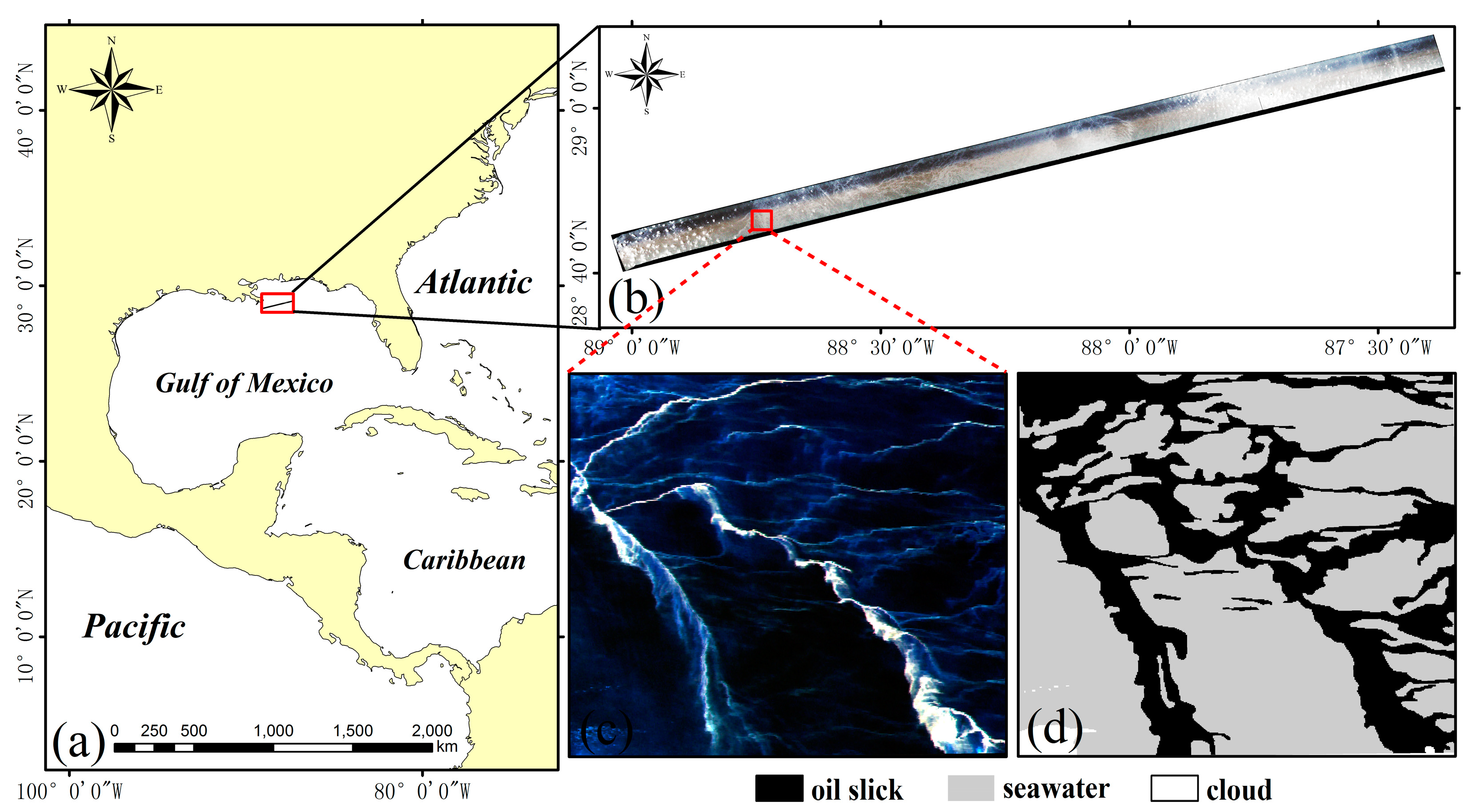
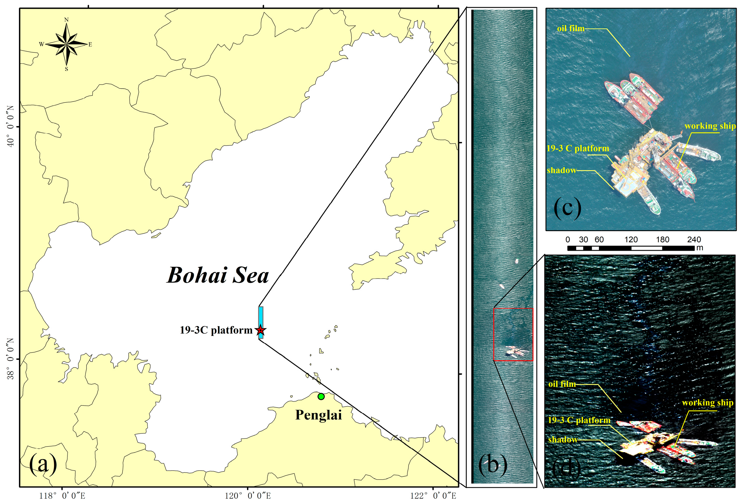
2.1. Accident Summary and AISA+ Hyperspectral Image

The formation pressure of platform B in the Penglai 19-3 oil field was excessively high owing to water injection on 4 June 2011, which led to crude oil leakage. A well kick accident occurred on 17 June because of improper drilling operations on the platform C, resulting in the overflow of crude oil and oil-based mud from the well into the sea. The accident polluted about 6200 km2 of sea area (exceeding the class I seawater quality standard), of which 870 km2 were seriously polluted (exceeding the class IV seawater quality standard) [2,48].
The AISA+ airborne imaging spectrometer of Finland’s Specim company was installed on the sea surveillance aircraft of the State Oceanic Administration for trial use in 2005, showing extensive application prospects in marine resource protection, environmental monitoring, and marine law enforcement. The hyperspectral image used in this study is an AISA+ airborne image covering the oil spill area of Penglai 19-3 platform C (Figure 1a) acquired by the China Marine Surveillance North Sea aviation detachment on 23 August 2011. Detailed parameters of the AISA+ hyperspectral sensor are listed in Table 1. Figure 1b is AISA+ radiance data without preprocessing such as atmospheric correction, band selection or dimensionality reduction, with the size of 3904 × 512 pixels, which is marked with a blue rectangle in Figure 1a. A study area of 444 × 364 pixels (Figure 1d) was clipped from the overall image, which is marked with a red rectangle in Figure 1b.

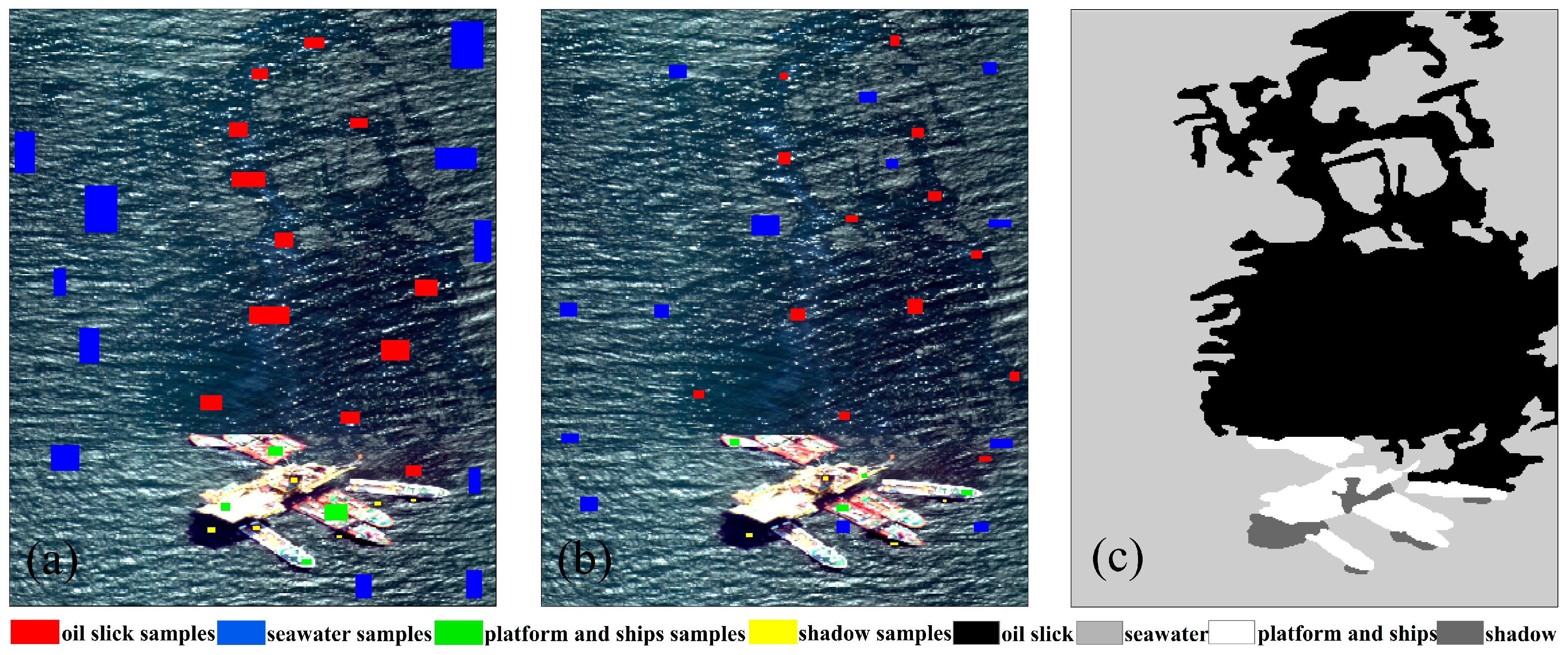
2.2. Sample Selection

Based on the field data, 9442 samples (pure pixels) were selected, including 7048 training samples for model establishment, and 2394 verification samples for adjusting the model parameters and determining the network structure. An interpretation map (Figure 2c) is made by the China Marine Surveillance North Sea aviation detachment, the marine oil spill operational monitoring department, according to field aerial photos (Figure 1c) combined with human-computer interactive methods. The interpretation map was used to test the performance of the optimal model by evaluating its generalization ability. The sample selection is shown in Table 2 and the spatial distribution is shown in Figure 2.

3. Method

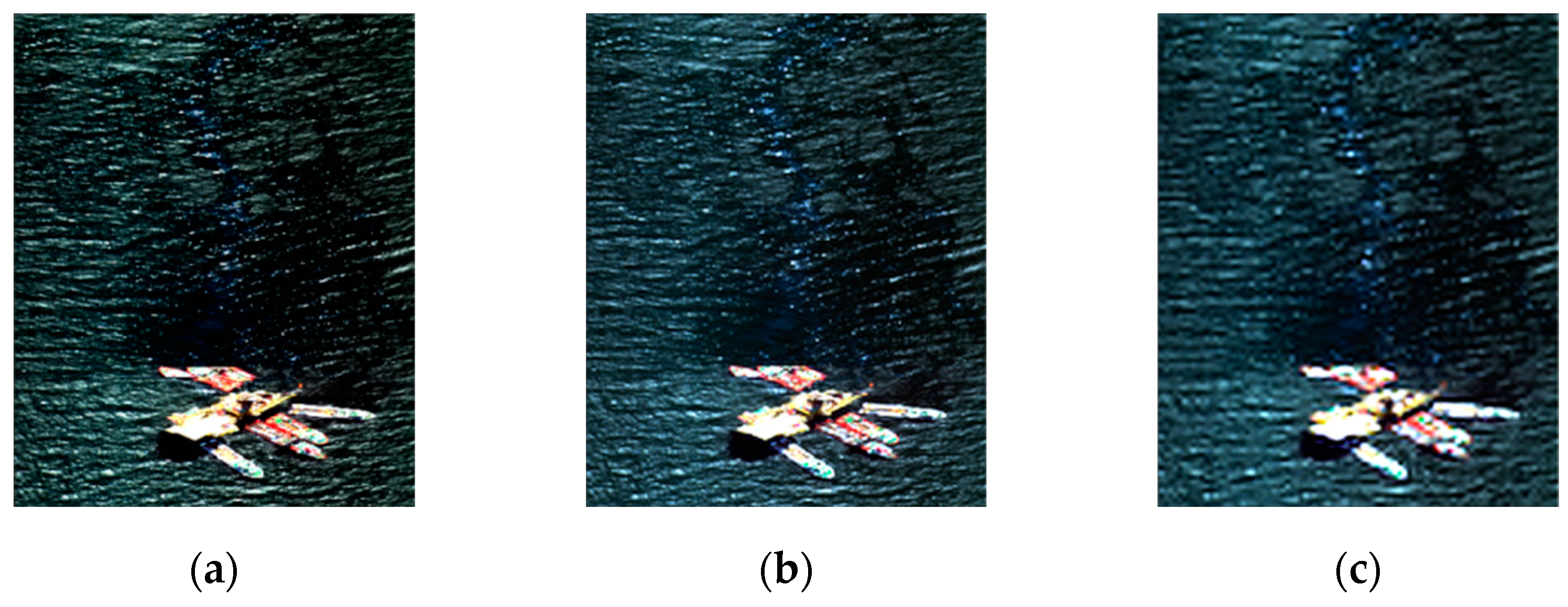
3.1. Multi-Scale Features Extraction Algorithm Based on Daubechies Wavelet

Due to the influence of sunlight and waves, there are fine ripples similar to oil slick in the sea water area, and fine ripples similar to seawater in the oil spill area, which will bring great error to oil spill detection. Discrete wavelet analysis method can not only separate the noise from the signal, but also highlight the characteristics of the original signal by decomposing the signal, whose essence is to extract image details by gradually thinning the sampling step in spatial domain, to separate the spatial feature images of different scales and to reflect them on the detailed images of different resolutions. Thus, wavelet transform has better scale characteristics.
In this paper, Daubechies (db) wavelet basis is selected as wavelet decomposition function to decompose hyperspectral data. In the first decomposition level, the original image is decomposed by wavelet transform into detail coefficients representing the high-frequency component and approximate coefficient representing the low-frequency component in the first scale space. Low-frequency component can save most of the low-frequency information of the image, smooth the spectral image, and eliminate the image noise. Then the approximate coefficient is decomposed into high-frequency coefficient and approximate coefficient in the second scale space. Finally, low-frequency component images of different scales are reconstructed through inverse wavelet transform. The 1-level and 2-level low-frequency component image are shown in Figure 3b,c, respectively.

3.2. Deep Learning Oil Spill Detection Algorithms Based on Multi-Scale Features

Hyperspectral images are characterized by the union of imagery and spectrum and contain rich spectral information. Deep learning has strong data mining ability and feature extraction ability and can automatically learn to obtain deep level feature information. Learned features are essential for data description to make classification more conducive.

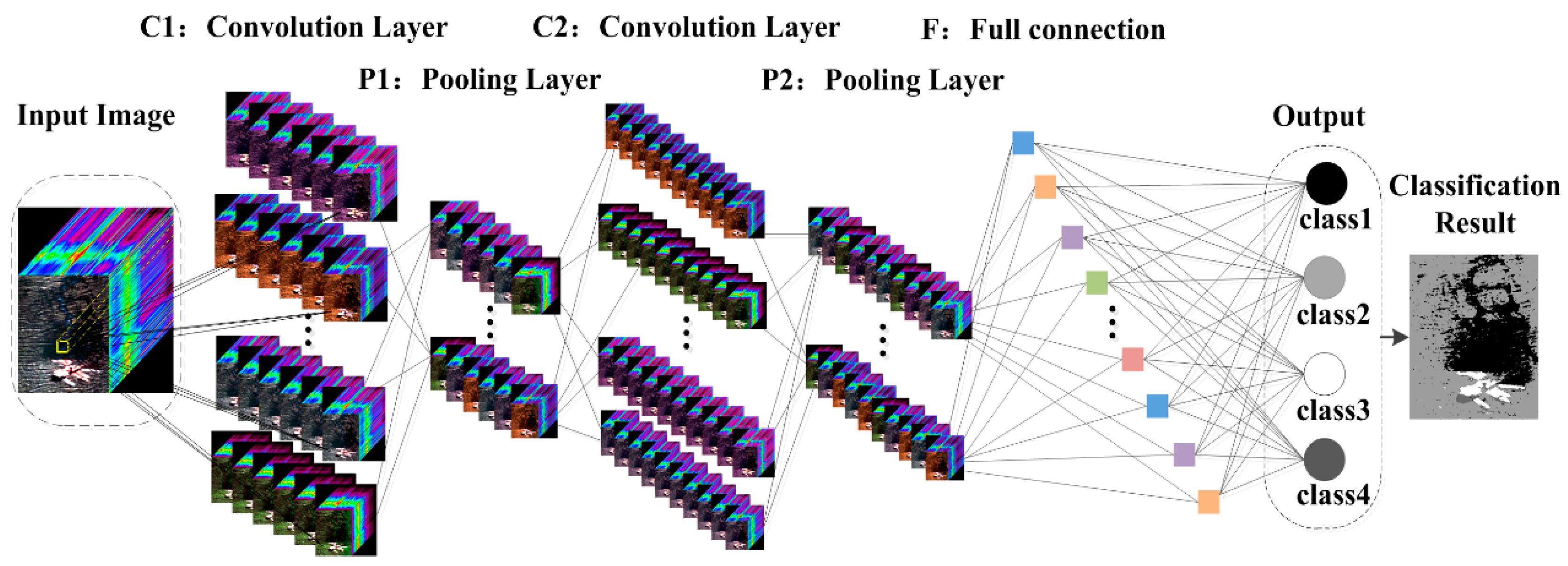
3.2.1. Convolutional Neural Network (CNN)

CNN is the most prominent model in deep learning and has recently become a research hotspot for hyperspectral remote sensing classification. CNN has two main characteristics. One is local receptive fields, i.e., hidden layer neurons that only connect with the local image, and global image information can be synthesized by each neuron’s local perception. The other is weight sharing, i.e., each neuron in the hidden layer uses the same convolution kernel to convolve the image, and all neurons in the same feature plane have the same weight, which effectively reduces the number of parameters in the network and makes CNN have displacement invariance. If the number of feature maps is too large, an over-fitting phenomenon occurs in the CNN model algorithm. The maximum pooling method is used to cluster features in different locations. The CNN model structure used in this paper is shown in Figure 4, which consists of seven information layers, including one input layer, two convolutional layers, two pooling layers, one full connection layer, and one output layer.
  • Convolutional Layer
Different convolution kernels are used to perform convolution operations to extract different features from the input feature map. Each convolution kernel detects the specific features at all locations and achieves weight sharing on the input feature map. The forward propagation of the convolutional layer is formulated as [34]
Q s t = f ( r V Q r t 1 k r s t + b s t ) ,
where Q s t represents the activation value of the output feature map s in layer t , V denotes a selection of input feature maps, k r s t is the kernel linking the input feature map r in layer t 1 to the output feature map s in layer t , b s t represents the bias associated with output feature map s in layer t , “ ” denotes convolutional multiplication, and f ( ) is the sigmoid function.
  • Pooling Layer
The pooling layers is also known as the subsampling layers, which are periodically introduced between convolutional layers, whose main purpose is to reduce the parameters of the output feature map from the convolutional layer and vaguely increase the rotation invariance of the features. The forward propagation of the convolutional layer is described as
Q s t = f ( m s t × d o w n ( Q s t 1 ) ) + b s t ,
where m s t denotes the multiplicative bias of the output feature map s in layer t , and b s t represents the additive bias of the output feature map s in layer t . Each output map is given its own multiplicative bias and additive bias. d o w n ( ) denotes a subsampling function. After the pooling operation, the resolution of the output feature map decreases but the features described by the high-resolution feature map are well maintained.

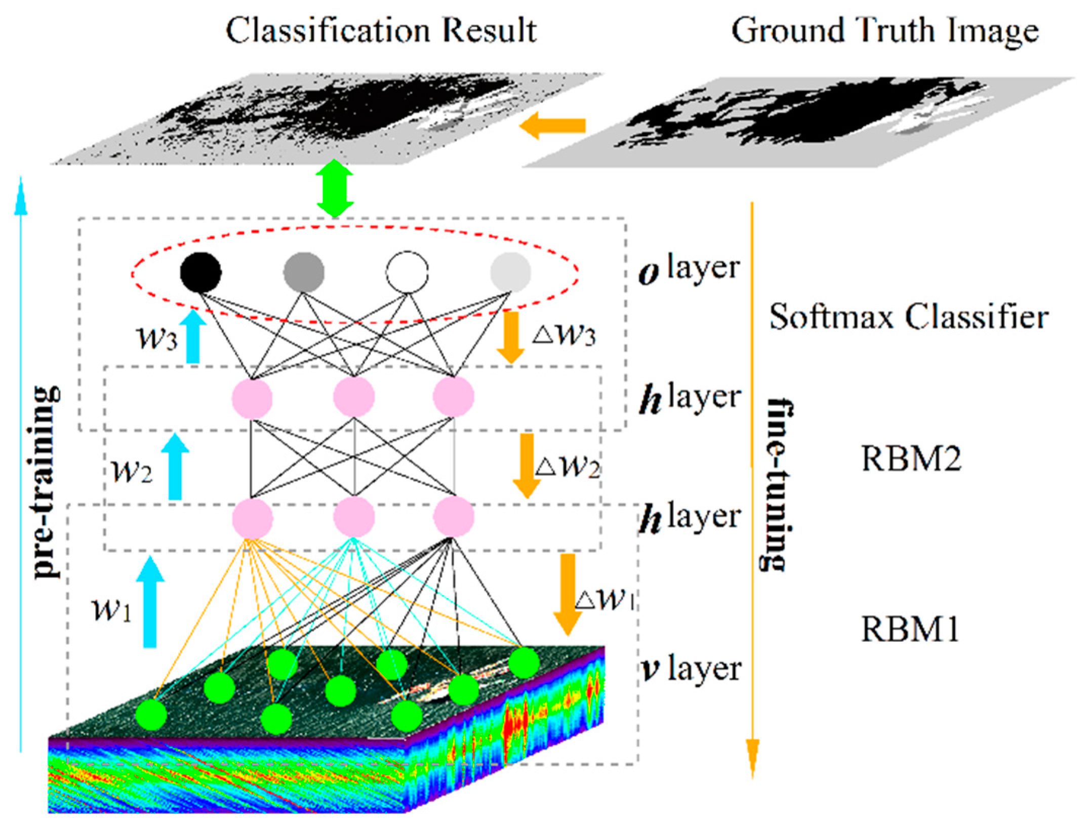
3.2.2. Deep Belief Network (DBN)

DBN combines forward unsupervised learning with reverse supervised learning, which can effectively restrain the over-fitting phenomenon of a neural network from occurring during classification. This improves the classification accuracy of the DBN model. The model is composed of a multilayer unsupervised Restricted Boltzmann Machine (RBM) and a layer of supervised back propagation network [39]. The classification process of the DBN model includes two stages: pre-training and fine-tuning. The DBN model structure used in this paper is shown in Figure 5, which consists of five information layers, including one input layer, one visible layers, two hidden layers, and one output layer.
The standard Boltzmann Machine is a full-connect graph and the training network is very complex. The vector s { 0 , 1 } n represents the state of n neurons, ω i j denotes the weight of the connection between visible-layer neuron i and hidden-layer neuron j , and θ i represents the threshold value of neuron i . The energy function E ( s ) [49] of the Boltzmann Machine corresponding to the state vector s is as follows. The occurrence probability P ( s ) of the state vector s is determined by its energy E ( s ) and energy of all possible state vectors E ( t ) :
E ( s ) = i = 1 n 1 j = i + 1 n ω i j s i s j i = 1 n θ i s i ,
P ( s ) = e E ( s ) t e E ( t ) ,
RBM only keeps the connection between the visible layer and hidden layer, and there is no self-feedback phenomenon in the layer. Thus, the structure of the Boltzmann Machine is simplified from a complete graph to a two-part graph [50]. Contrastive divergence (CD) is often used to train RBM [51]. Suppose there are d visible-layer neurons and q hidden-layer neurons in the network, and υ and h represent state vector of visible layer and hidden layer, respectively. Because there is no connection in the same layer, then
P ( ν | h ) = i = 1 d P ( ν i | h ) ,
P ( h | ν ) = j = 1 q P ( h i | ν ) ,
For each training sample ν , the probability distribution of the neuron state in the hidden layer can be calculated by the CD algorithm according to Equation (6), and then h can be obtained by sampling according to probability distribution. Similarly, ν is generated from h according to Equation (5), and then h is generated from ν . The updated formula of connection weight is
Δ ω = η ( ν h T ν h T ) ,
The forward learning process of the DBN model is the process of feature extraction. When RBM maps feature information of neurons in the visible layer, each neuron in the hidden layer of the RBM has the same probability of being activated. Features of the neurons in the visible layer can be accurately expressed after several training times. In this case, RBM can be regarded as a self-encoder to extract feature information of neurons in the visible layer.
In the pre-training process, the DBN model carries out forward training through layer by layer initialization, and maps and transmits the characteristic information of the input layer data by stacking RBM layers. In this paper, a softmax classifier is set at the top of the top-level RBM, which receives the output information of the top-level RBM as the input information. The softmax classifier outputs the classification results of the forward learning process by comparing the probability distribution. In the process of fine-tuning, on the basis of pre-training, each layer of RBM network can only ensure that the weight of this layer can achieve the optimal expression of the characteristic information of this layer, and cannot achieve the optimal mapping of the whole DBN model to the input information. Therefore, BP algorithm needs to be used to combine with forward unsupervised classification results and label data, and fine tune the connection weight and bias between neurons in each layer of the whole DBN model layer by layer from the top to the bottom according to the law of error back propagation.

3.3. Classical Shallow Learning Algorithms

Shallow learning usually refers to shallow neural network, but here refers to methods other than deep learning algorithms. The occurrence time of oil spill events is often uncertain, which makes oil spill data difficult to obtain. Classical shallow learning methods have better performance for smaller datasets and are more easily understood.

3.3.1. Support Vector Machine (SVM)

SVM is a shallow learning method based on statistical learning theory. It can automatically find the support vector that has a greater ability to distinguish classification and then construct the classifier, which can maximize the interval between classes to achieve good statistics when the number of samples is small. This method has high convergence efficiency, training speed, and classification accuracy, and has been widely used in many fields of research in recent years [52,53]. The kernel function is the radial basis function (RBF) and the decision function is
f ( x ) = sgn ( i = 1 n ω i e ( γ x i x 2 ) + b ) ,
where ω i represents the coefficient of support vector, γ is the parameter in the kernel function, the value here is 0.004, x i is the support vector, x are samples of labels to be predicted, and b is the offset coefficient.

3.3.2. Mahalanobis Distance (MD)

Mahalanobis Distance represents the distance between a point and a distribution, which is an effective method to calculate the similarity of two unknown sample sets. Its calculation is based on the overall sample. Different from Euclidean Distance, Mahalanobis distance takes into account the relationship between various characteristics, and can eliminate the interference of correlation between variables. Its disadvantage is that it exaggerates the effect of small variable.

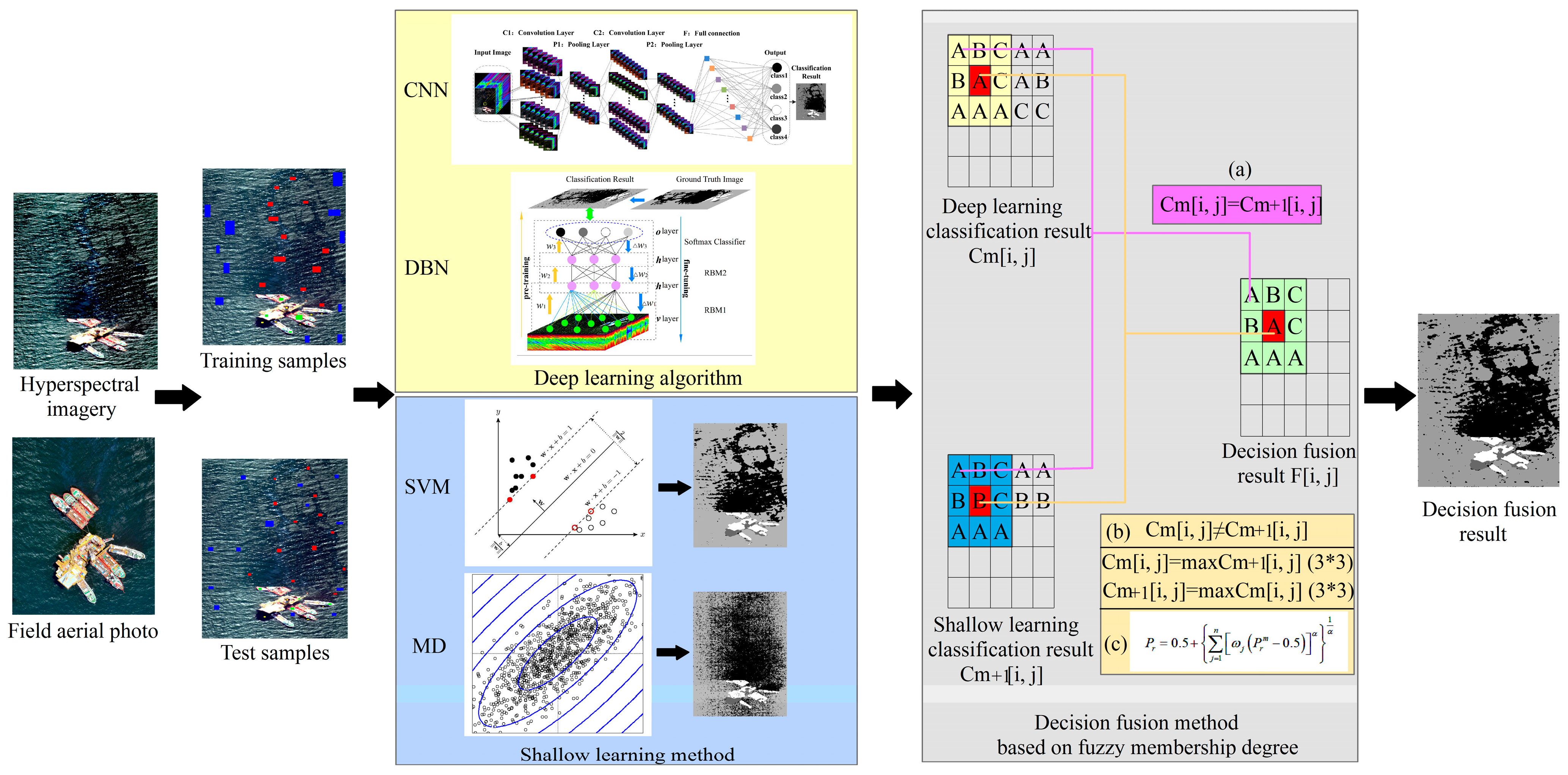
3.4. Decision Fusion Method Based on Fuzzy Membership Degree

In this paper, the decision fusion algorithm based on fuzzy membership degree is used to realize the fusion of multi-source oil spill information obtained by deep learning model and shallow learning method [35]. The basic idea (Figure 6) is: (a) the detection results C m and C m + 1 of two classifiers are compared and if the pixel types in the same position are the same, (i.e., C m [ i , j ] = C m + 1 [ i , j ] ), then the fusion image pixel types remain unchanged. (b) If the types are different, then the class max C m + 1 with the largest number of object types in the window with a pixel size of 3 × 3 centered on the pixel is counted to determine whether the class is the same as that of the pixel in the corresponding position in another image, (i.e., C m [ i , j ] = max C m + 1 ), then the fusion pixel is F [ i , j ] = C m [ i , j ] . Similarly, if max C m + 1 is different from C m [ i , j ] , the relationship between max C m and C m + 1 [ i , j ] is calculated. If C m + 1 [ i , j ] = max C m , then the fusion pixel is F [ i , j ] = C m + 1 [ i , j ] . (c) When the pixel category cannot be discriminated, the membership degree P r m that the pixel m belonging to category r is calculated according to Equation (9). If the maximum membership degree meets certain conditions, then the category with the largest membership degree is selected as the final category of the pixel.
P r = 0.5 + { j = 1 n [ ω j ( P r m 0.5 ) ] α } 1 α ,
where P r denotes the degree of belonging of type r , the range of category r is [1,4] in the experiment, that is, four categories, and n represents the number of classification images, ω j denotes the weight of each single objective feature, and satisfies the equation of j = 1 n ω j = 1 . α is odd, and the classification accuracy of the two classifiers is a and b , respectively. Then, ω 1 = a a + b and ω 2 = b a + b .

4. Results

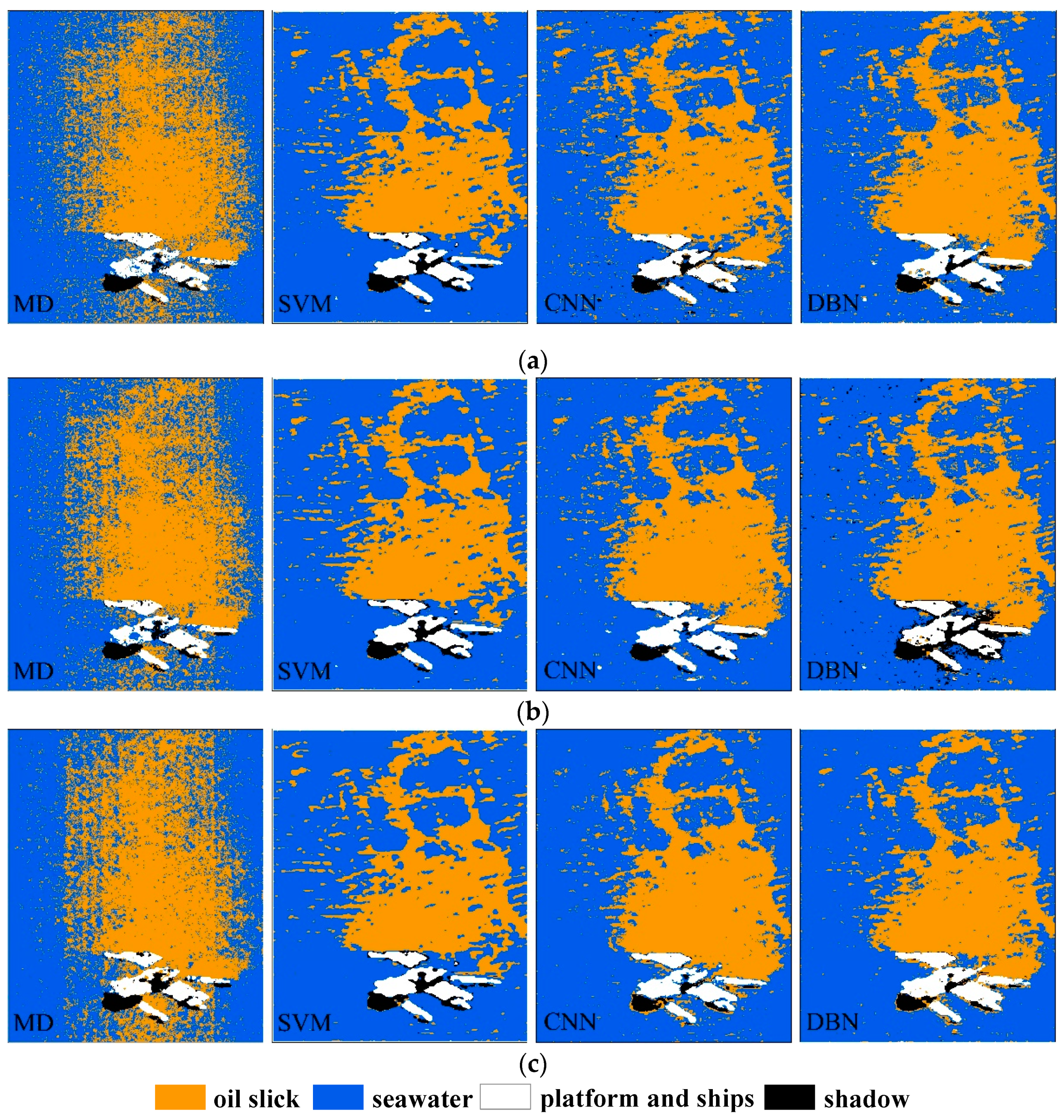
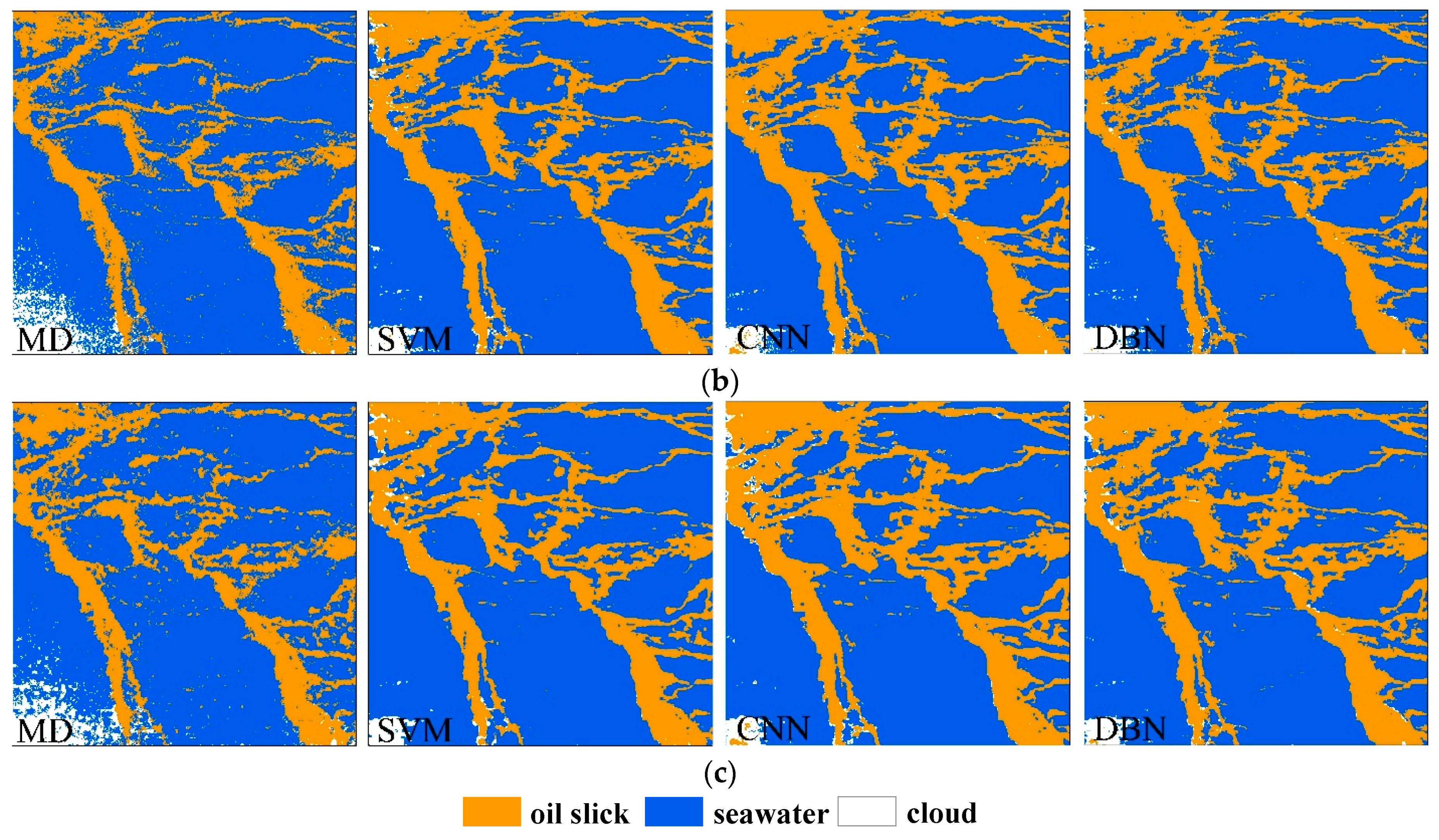
4.1. Oil Spill Detection Results of Single Classifier under Different Scales

Aiming at three scale features, namely the original image (original scale), the low-frequency component image after 1-level wavelet transform combined with the original image (first-level scale), and the low-frequency component image after 1-level and 2-level wavelet transform combined with the original image (second-level scale), two deep learning methods and two shallow learning methods are used to extract the oil spill information based on the same training samples (Table 2), detection results are shown in Figure 7. Two deep learning models and two shallow learning classifiers have different abilities in mining data feature, and the performance of oil spill detection is also different. Intuitively, there is no obvious boundary between oil film and seawater in the detection results with different scales of MD algorithm, and there is more speckle noise, which is quite different from the interpretation map (Figure 2c) obtained by human–computer interaction. The oil film patches in the detection results of SVM based on different scale features are discontinuous, and some seawater pixels are mistakenly divided into platform and ship pixels. The detection results with different scales of CNN and DBN algorithms can keep the continuity of the oil film on the sea surface well. The detection results of CNN and DBN based on the first-level scale feature are more consistent with the interpretation map obtained by human–computer interaction, and effect is the best (Figure 7b). Some seawater pixels are mistakenly divided into oil film pixels in CNN and DBN detection results based on second-level scale characteristics (Figure 7c). These differences are the basis of data complementarity using decision fusion method, and also the significance of decision fusion of deep learning method and shallow learning method. The specific analysis will be described in combination with the accuracy evaluation later.

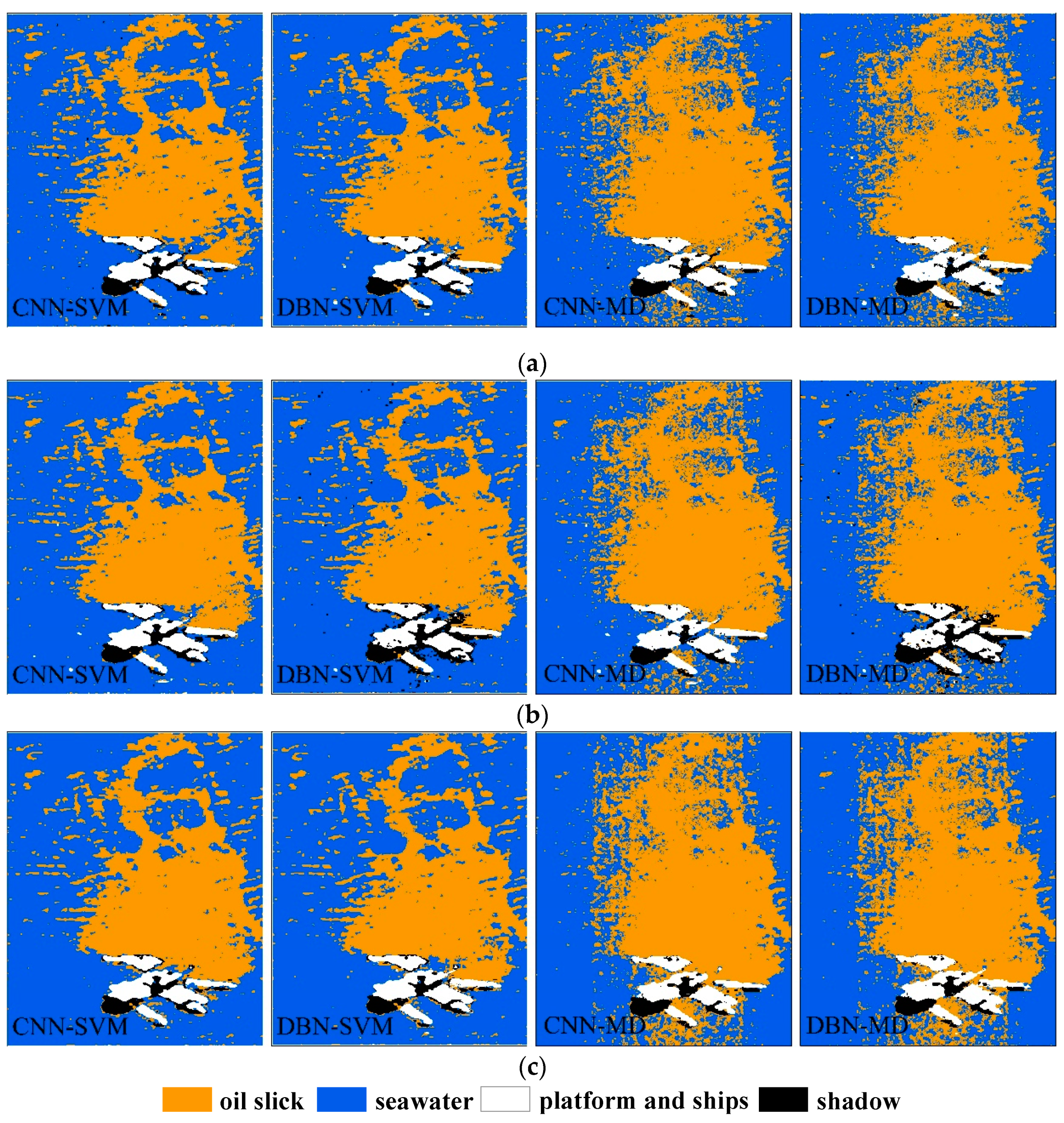
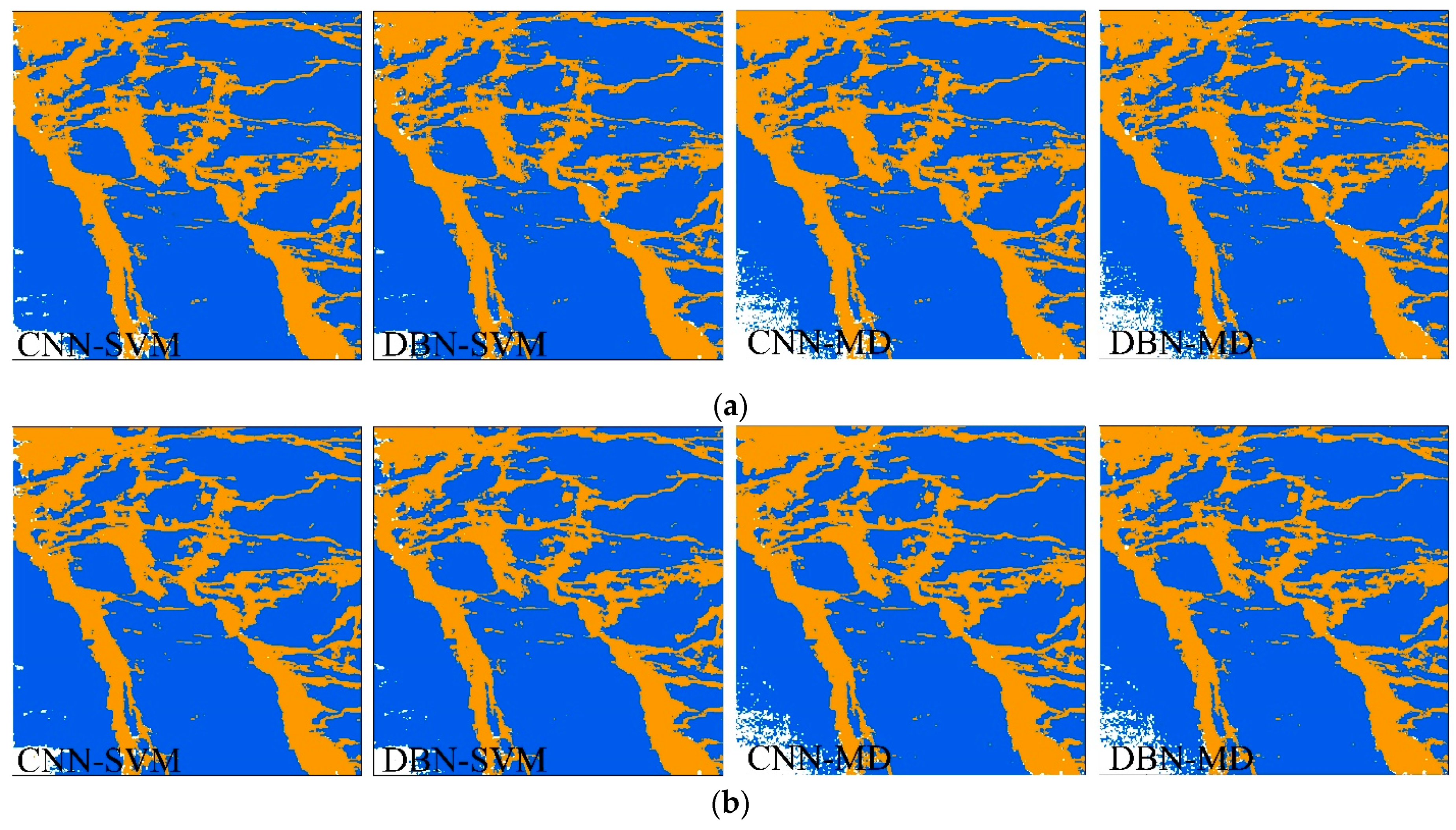
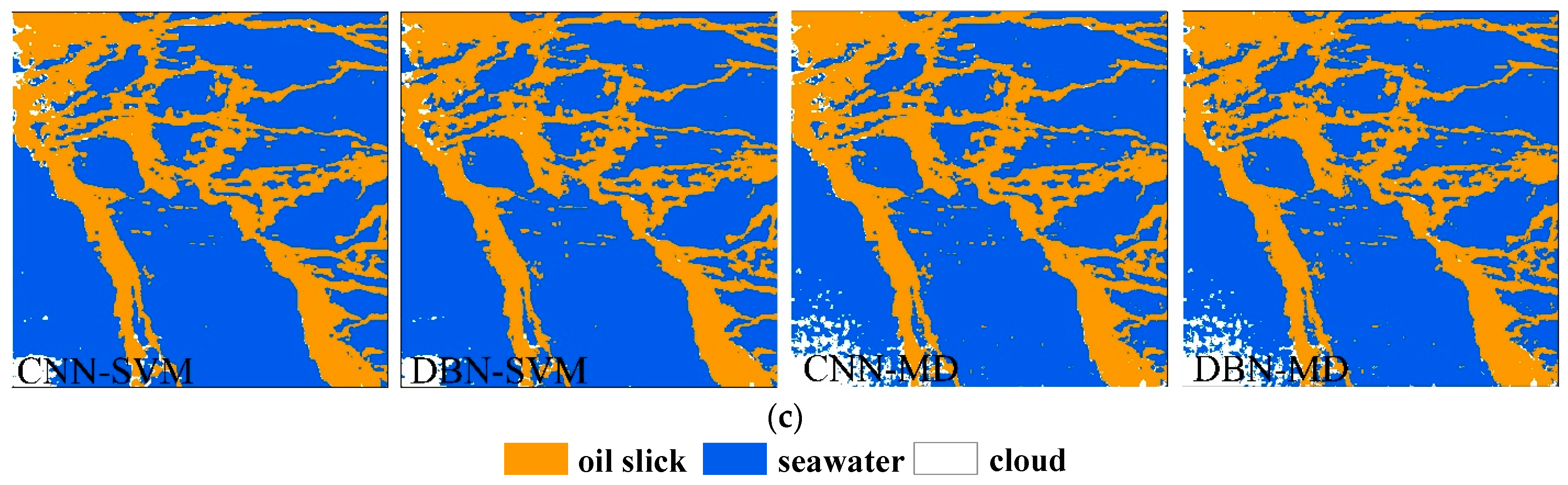
4.2. Experimental Results of Decision Fusion

Based on the oil spill detection results of two deep learning algorithms CNN and DBN, and two shallow learning algorithms SVM and MD, the decision fusion algorithm is introduced to fuse the oil spill information from the perspective of target recognition information fusion. The fusion results are shown in Figure 8. Compared with the single classifier, the oil film in the decision fusion results of deep learning and shallow learning at different scales is more continuous, and there are fewer broken patches, and the detection effect of the oil film is improved to varying degrees. Among them, decision fusion results based on the first-level scale features of two deep learning algorithms and SVM match the interpretation graph best (Figure 8b). Decision fusion detection results of MD, CNN and DBN algorithm at different scale feature can overcome the problem that there is no obvious boundary between oil film and seawater in MD detection results. At the same time, they inherit the characteristics of single classifier detection results and still have more speckle noise.

5. Discussion

5.1. Accuracy Evaluation of Oil Spill Detection

Precision and Recall are two measures widely used in statistical classification to evaluate the quality of classification results. Precision represents the ability of the classification model to return only relevant instances. Recall represents the ability of the classification model to identify all relevant instances, but sometimes there is a contradiction between Precision and Recall. To effectively evaluate the advantages and disadvantages of the different algorithms, the F1 score, also known as the balanced F score, is introduced to harmonize Precision and Recall. The F1 score has a better evaluation ability for a binary classification problem. Here, the detection performance of different algorithms is evaluated for the single target of the oil film.
Table 3 shows that on the basis of different scale feature images, compared with the shallow learning method, two deep learning methods have higher detection accuracy, among which CNN algorithm has the highest detection accuracy, followed by the DBN algorithm, and MD has the lowest detection accuracy. The detection accuracy of CNN algorithm based on the first-level scale features is the highest, with F1 value of 0.8715. This proves that the deep-seated feature information extracted by deep learning model is more conducive to oil spill detection. At the same time, we can find that for MD, CNN, and DBN, detection accuracies based on the first-level scale features are the highest, with F1 values of 0.7154, 0.8715, and 0.8635, respectively. The detection accuracy of SVM algorithm increases with the increase of scale, and optimal detection accuracy is 0.8524. For SVM, CNN, and DBN, detection accuracies based on the first-level scale and the second-level scale features are better than that based on the original scale feature. The existence of strong solar flares will interfere the accurate detection of oil spill on the sea surface. The low-frequency components of different scales generated by wavelet transform can eliminate image noise and improve the accuracy of oil spill detection to a certain extent.
It can be seen from Table 4 that under the same scale feature, detection accuracies of decision fusion results of deep learning and shallow learning methods are better than those of single classifiers. For example, the F1 value of CNN and SVM decision fusion results based on original scale features is 0.8720, while the oil spill detection accuracy of CNN and SVM is 0.8489 and 0.8452, respectively; the F1 value of decision fusion result of CNN and SVM based on the first-level scale feature is 0 8801, while the accuracy of CNN and SVM based on the first-level scale feature is 0.8715 and 0.8513, respectively. Oil spill detection accuracies for decision fusion of SVM and two deep learning methods based on different scale features are higher than those of MD and two deep learning methods. Decision fusion results of CNN and SVM (CNN-SVM) have the highest detection accuracy, decision fusion results of DBN and SVM (DBN-SVM) take the second place, and decision fusion results of CNN and MD (CNN-MD) has the lowest detection accuracy, which shows that two single classifiers with better oil spill detection accuracy will have higher detection accuracy of decision fusion. At the same time, we can find that in the decision fusion results of deep learning and shallow learning methods, detection accuracies based on the first-level scale feature are the highest, followed by the original scale feature, and detection accuracies based on the second scale feature are the lowest, which is related to the better oil spill detection effect of single classifiers under the first-level scale feature. The decision fusion algorithm uses the complementarity of single deep learning model and shallow learning classifier, and uses the fusion strategy to give full play to the advantages of different classifiers, and further improves the accuracy of oil spill detection on the sea surface.

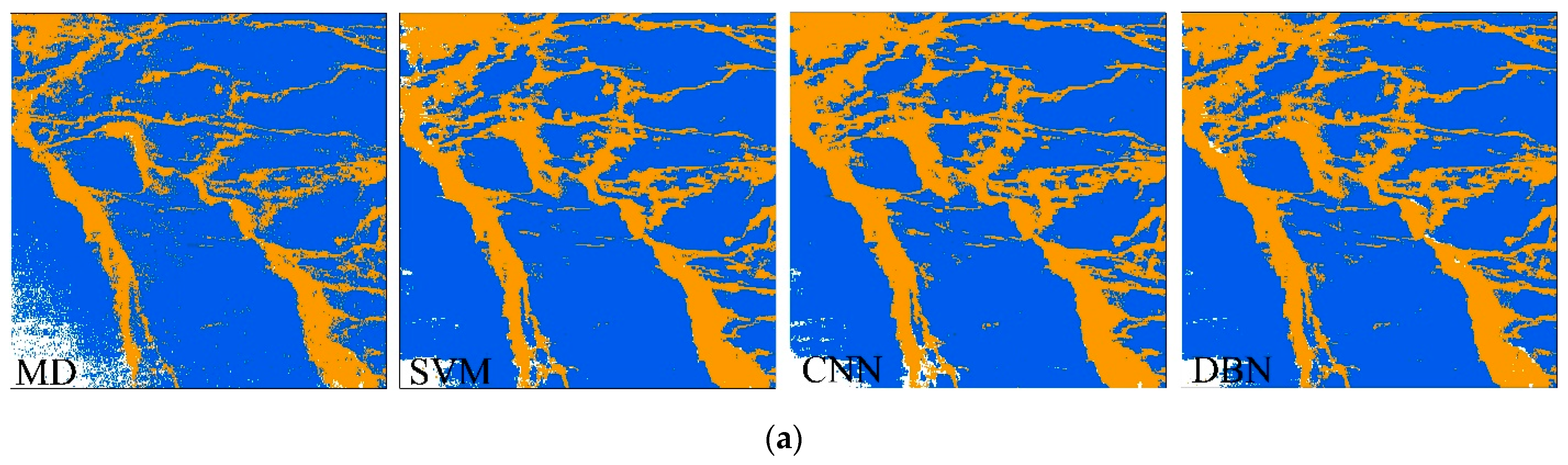
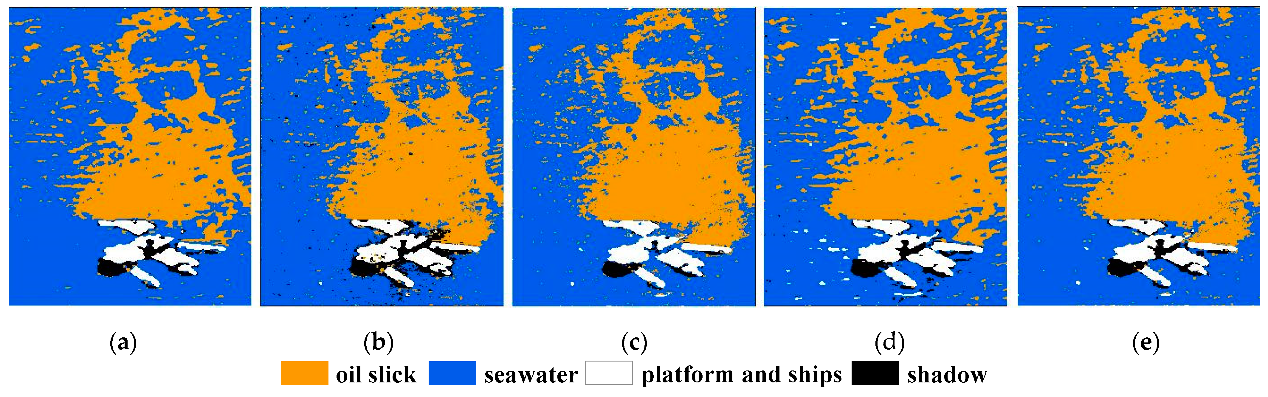
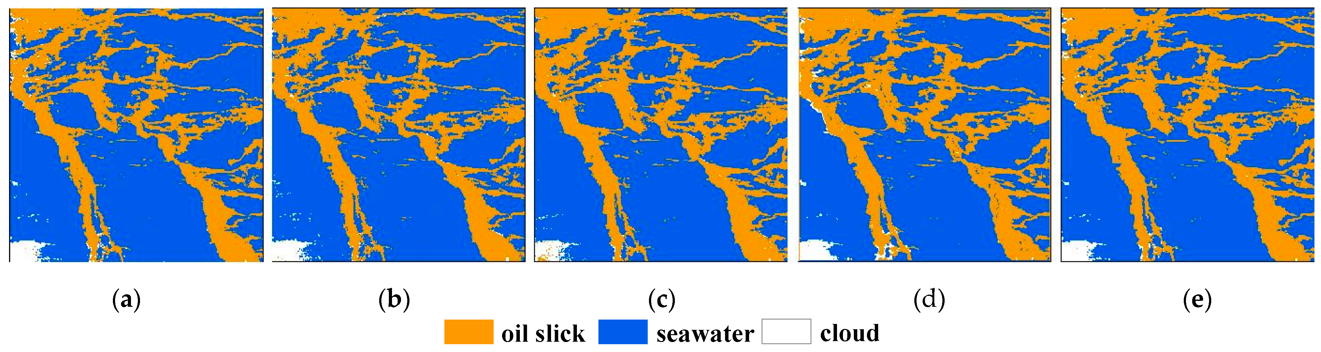
5.2. AVIRIS Hyperspectral Application of the Proposed Method

In order to verify the effectiveness and applicability of the proposed decision fusion method, in this section, we apply the algorithm to the 2010 AVIRIS oil spill hyperspectral data of the Gulf of Mexico. Figure 9a shows the location of the oil spill image. The AVIRIS image (Figure 9b) has 224 bands, with spectral resolution of 10 nm and spatial resolution of 0.89 m@1 km. The spectral range is 350–2500 nm, covering visible, near-infrared and shortwave infrared spectra. The field of view of the sensor is 34°. The imaging time of the AVIRIS oil spill hyperspectral imagery is 18 May 2010, and the scene size is 400 × 400 (Figure 9c). The AVIRIS image input into the model is radiance data without preprocessing steps such as atmospheric correction, band selection or dimensionality reduction.
There are three types of ground truth samples in this image. The number of training samples and test samples for each class is shown in Table 5.
We carry out oil spill detection experiment by our proposed decision fusion algorithm. Oil spill detection results of MD, SVM, DBN, and CNN based on different scale features using the same training samples are shown in Figure 10, and their decision fusion results at different scales are shown in the Figure 11. The F1 score is used as an indicator for accuracy evaluation. The accuracies for oil spill detection of four methods based on different scale features are listed in Table 6, and the detection accuracies of their decision fusion results are listed in Table 7.
Table 6 shows that CNN and DBN have higher detection accuracy than the shallow learning methods, among which CNN algorithm has the highest detection accuracy, followed by the DBN algorithm, and MD has the lowest detection accuracy. The detection accuracy of CNN algorithm based on the first-level scale features is the highest, with F1 value of 0.8904. At the same time, we can find that no matter which method is used, the detection accuracy based on the first-level scale feature image is better than that based on the original scale feature.
It can be seen from Table 7 that under the same scale feature, detection accuracies of decision fusion results of deep learning and shallow learning methods are better than those of single classifiers. For example, the F1 value of CNN and SVM decision fusion results based on the original scale features is 0.8915, while the oil spill detection accuracy of CNN and SVM is 0.8857 and 0.8705, respectively. At the same time, we can find that in the decision fusion results of deep learning and shallow learning methods, detection accuracies based on the first-level scale feature are the highest, followed by the original scale feature, and detection accuracies based on the second scale feature are the lowest.
Through the above analysis of oil spill AVIRIS detection experiments, we can draw the same conclusion with the previous ones using AISA+ data, which show that the developed decision fusion method has an applicability in different oil spill scenarios, and can detect the oil spill on the sea surface.

5.3. Satellite Hyperspectral Application of the Proposed Method

Up to now, hyperspectral remote sensing technology has been widely used in many fields, such as environmental monitoring, atmospheric exploration, earth resources survey and natural disasters monitoring. Marine oil spill is a kind of emergent incident, which requires the operational departments to respond quickly. Airborne hyperspectral remote sensing has the characteristics of flexibility, fast acquisition, high spatial and spectral resolution. Therefore, airborne hyperspectral sensors have an advantage in obtaining oil spill image in time. However, due to the limitation of weather conditions, it is difficult to acquire aerial data, especially during oil spill accidents. The advantages of spaceborne hyperspectral remote sensing are: (a) continuity, (b) consistency, and (c) global coverage. Although spaceborne hyperspectral remote sensing have some advantages, and many satellite hyperspectral sensors (such as EO-1 Hyperion, ISS HICO, and GF-5 AHSI, etc.,) are still in service, but they also face some challenges, such as cloud, low spatial resolution, narrow swath, long revisit period, and low signal-to-noise ratio. It is exciting that a new generation of hyperspectral satellites (PRISMA and EnMAP) may provide better data. The main parameters of several airborne and spaceborne hyperspectral imagers are listed in Table 8.
In order to verify the portability of this method on hyperspectral satellite data, we apply the developed decision fusion algorithm to the oil spill hyperspectral data of Liaodong Bay in 2007, which is obtained by EO-1 Hyperion (Figure 12). The Hyperion hyperspectral image has 242 bands in total, of which 198 bands are radiometric calibrated, while bands 1–7, 58–76, and 225–242 are 0, which must be removed. At the same time, due to the influence of signal-to-noise ratio and water vapor, 19 bands also need to be eliminated. In the experiment, Hyperion image containing 179 bands are used. The spectral range is 350–2500 nm, spectral resolution of 10 nm, and spatial resolution of 30 m. However, the image contains a lot of stripe noise and bad lines, which seriously affect the oil spill detection. It is indicated from Figure 13, the oil spill detection effects of the four algorithms are poor due to the stripe noise and bad lines of the image. However, this does not mean that our method cannot be applied to hyperspectral satellite data of oil spill. We plan to apply this method to other hyperspectral satellite data with high imaging quality to prove the feasibility of this method on satellite records.

5.4. Comparison with Other Algorithms

To further evaluate the effect of the algorithm proposed in this study, four mainstream algorithms such as SVM, DBN [39], 1D-CNN [38], and MRF-CNN [54] were chosen for comparative analysis and evaluation. The MRF-CNN (Markov Random Field-Convolutional Neural Networks) regional fusion decision strategy exploited the complementary characteristics of the two classifiers, which can overcome the problem of losing effective resolution and uncertain prediction at object boundaries, which is especially pertinent for complex fine spatial resolution image.
During the experiment, the parameters of the four comparison algorithms were set as the default values corresponding to the parameter settings in the study. Oil spill detection results for each algorithm based on AISA+ and AVIRIS hyperspectral images are shown in Figure 14 and Figure 15, respectively. Compared with other four algorithms, the oil film in the experimental results obtained by the algorithm proposed in this paper is more continuous, and there are fewer broken patches, and the detection effect of the oil film is improved to varying degrees. Oil spill detection accuracy of each algorithm is shown in Table 9. The overall classification accuracy (OA) and F1 score of the algorithm proposed in this study were higher than those of the SVM, DBN, 1D-CNN, and MRF-CNN algorithms. The improvement of F1 score was 0.0277, 0.0166, 0.0086, and 0.0129, respectively. The overall classification accuracy of the proposed method is 2.03%, 2.15%, 1.32%, and 0.43% higher than that of the other four algorithms, respectively.

5.5. Other Considerations

Whether for single-target detection or multi-target classification, the decision fusion algorithm based on fuzzy membership degree integrates the advantages of multiple single classification algorithms from the perspective of target recognition information fusion, and the classification accuracy of fusion results is improved, which shows that the algorithm is practical and effective. On the premise of existing single classifier resources, it is an important way to improve the classification accuracy of hyperspectral images. When an oil spill accident in marine occurs, remote sensing is an important means to detect the oil spill on the sea surface in a large scale, especially the aerial optical remote sensing, which can provide oil spill information timely and effectively. However, due to the limitation of observation geometry and the influence of sea waves, sun glints will inevitably appear in airborne images, which will interfere the oil slick detection. Although the discrete wavelet analysis method can produce different scale features by decomposing the signal, and eliminate part of the noise, it cannot completely suppress the influence of sun glints. This experiment is an attempt to use decision fusion algorithm of deep learning models and shallow learning methods based on different scale feature for oil spill detection. In the near future, we plan to use other solar flare suppression methods combined with decision fusion to carry out experiments, and compare with other decision fusion methods to further highlight the advantages of the decision fusion algorithm.

6. Conclusions

Aiming at the oil spill event of Penglai 19-3 platform in 2011, based on the airborne AISA + hyperspectral image and the multi-scale features after wavelet transform, this paper uses two deep learning methods and two shallow learning methods to extract the oil spill information at three different scales. Based on oil spill detection results of single algorithms, the decision fusion algorithm based on fuzzy membership degree is used to fuse multi-source oil spill information under the same scale. The main conclusions are as follows: (1) oil spill detection accuracies of deep learning methods based on different scale features are higher than those of shallow learning methods with corresponding scale, which proves that the deep-seated feature information extracted by deep learning model is more suitable for oil spill detection on sea surface. (2) At the same scale, the decision fusion algorithm based on fuzzy membership has better oil spill detection performance than those of single classifiers. For instance, oil spill detection accuracy (F1 value) using decision fusion algorithm based on the original scale feature is 0.8720, which is improved by 0.025 on average than that of the state-of-art single algorithms. (3) For single detection algorithms, oil spill detection accuracies based on the first-level scale feature and the second-level scale feature are better than those based on the original scale feature. For decision fusion results of deep learning and shallow learning methods, oil spill detection accuracies based on the first-level scale feature are the highest, followed by the original scale, and detection accuracies based on the second-level scale feature are the lowest. (4) The overall classification accuracy of the proposed method is 91.93%, which is 2.03%, 2.15%, 1.32%, and 0.43% higher than that of SVM, DBN, 1D-CNN, and MRF-CNN algorithms, respectively. The improvement of F1 score is 0.0277, 0.0166, 0.0086, and 0.0129, respectively.
The algorithm developed in this paper is an oil spill detection model based on the decision fusion of shallow learning and deep learning. The detection results of the developed model depend on the classification results of the basic classifiers to a certain extent, that is, the detection results of shallow learning algorithm and deep learning algorithm. Therefore, in a practical application, the selection of basic classifiers is particularly important. It is necessary to select basic classifiers with strong feature extraction ability in order to make the oil spill detection accuracy of decision fusion based on fuzzy membership better. Rapid and effective monitoring of the location and range of the oil spill is very important for rapid response. With the development of unmanned aerial vehicle (UAV) technology, it is a trend to apply oil spill detection algorithm to UAV system to realize real-time oil spill detection. At the same time, the coordination of multi-source remote sensing for marine oil spill detection is also the research direction in the future.

Author Contributions

Conceptualization, J.Y. and Y.M.; methodology, J.Y., Y.M. and Y.H.; software, J.Y., Y.H. and Z.J.; validation, J.Y. and Y.H.; formal analysis, J.Y.; data curation, J.Y.; writing—original draft preparation, J.Y.; writing—review and editing, J.Y., Y.M. and J.W.; supervision, Y.M. and J.W.; project administration, Y.M., J.W., J.Z. and Z.L.; funding acquisition, Y.M., J.Z. and Z.L. All authors have read and agreed to the published version of the manuscript.

Funding

This research was funded by the National Natural Science Foundation of China (Grant No. 61890964, U1906217, 42106179, 42076182) and the Independent Innovation Research Project of China University of Petroleum (Grant No. 21CX06057A).

Institutional Review Board Statement

Not applicable.

Informed Consent Statement

Not applicable.

Data Availability Statement

The data used in this study are available on request from the first author.

Acknowledgments

We thank China Marine Surveillance North Sea Aviation Detachment and the U.S. National Aeronautics and Space Administration (NASA) for providing AISA+ data and AVIRIS data (https://aviris.jpl.nasa.gov/, accessed on 17 January 2020). We thank Esther Posner, from Liwen Bianji, Edanz Editing China (www.liwenbianji.cn/ac, accessed on 10 July 2021), for improving this manuscript. We would like to express our sincere appreciation to anonymous reviewers who provided valuable comments to help improve this paper.

Conflicts of Interest

The authors declare no conflict of interest.

References

  1. Leifer, I.; Lehr, W.J.; Simecek-Beatty, D.; Bradley, E.; Clark, R.; Dennison, P.; Hu, Y.X.; Matheson, S.; Jones, C.E.; Holt, B. State of the art satellite and airborne marine oil spill remote sensing: Application to the BP Deepwater Horizon oil spill. Remote Sens. Environ. 2012, 124, 185–209. [Google Scholar] [CrossRef] [Green Version]
  2. Yang, J.F.; Ma, Y.; Ren, G.B.; Dong, L.; Wan, J.H. Oil spill AISA+ hyperspectral data detection based on different sea surface glint suppression methods. In Proceedings of the ISPRS XLII-3, Beijing, China, 7–11 May 2018. [Google Scholar]
  3. Yang, J.F.; Wan, J.H.; Ma, Y.; Hu, Y.B. Research on Objected-Oriented Decision Fusion for Oil Spill Detection on Sea Surface. In Proceedings of the IEEE International Geoscience and Remote Sensing Symposium (IGARSS), Yokohama, Japan, 28 July–3 August 2019. [Google Scholar]
  4. Cally, C. Unique oil spill in East China Sea frustrates scientists. Nature 2018, 554, 17–18. [Google Scholar]
  5. Lu, Y.C.; Li, X.; Tian, Q.J.; Zheng, G.; Sun, S.J.; Liu, Y.X.; Yang, Q. Progress in Marine Oil Spill Optical Remote Sensing: Detected Targets, Spectral Response Characteristics, and Theories. Mar. Geod. 2013, 36, 334–346. [Google Scholar] [CrossRef]
  6. Fingas, M.; Brown, C. Review of oil spill remote sensing. Mar. Pollut. Bull. 2014, 83, 9–23. [Google Scholar] [CrossRef] [PubMed] [Green Version]
  7. López-Peña, F.; Duro, R.J. A Hyperspectral Based Multisensor System for Marine Oil Spill Detection, Analysis and Tracking. In Proceedings of the 8th International Conference of Knowledge-Based Intelligent Information and Engineering Systems, Wellington, New Zealand, 20–25 September 2004. [Google Scholar]
  8. Zhao, D.; Cheng, X.; Zhang, H.; Niu, Y.; Qi, Y.; Zhang, H. Evaluation of the ability of spectral indices of hydrocarbons and seawater for identifying oil slicks utilizing hyperspectral images. Remote Sens. 2018, 10, 421. [Google Scholar] [CrossRef] [Green Version]
  9. El-Rahman, S.A.; Zolait, A.H.S. Hyperspectral image analysis for oil spill detection: A comparative study. Int. J. Comput. Sci. Math. 2018, 9, 103–121. [Google Scholar] [CrossRef]
  10. Khanna, S.; Santos, M.J.; Ustin, S.L.; Shapiro, K.; Haverkamp, P.J.; Lay, M. Comparing the potential of multispectral and hyperspectral data for monitoring oil spill impact. Sensors 2018, 18, 558. [Google Scholar] [CrossRef] [Green Version]
  11. Dilish, D. Spectral similarity algorithm-based image classification for oil spill mapping of hyperspectral datasets. J. Spectr. Imaging 2020, 9, a14. [Google Scholar]
  12. Wettle, M.; Daniel, P.J.; Logan, G.A.; Thankappan, M. Assessing the effect of hydrocarbon oil type and thickness on a remote sensing signal: A sensitivity study based on the optical properties of two different oil types and the HYMAP and Quickbird sensors. Remote Sens. Environ. 2009, 113, 2000–2010. [Google Scholar] [CrossRef]
  13. Lu, Y.C.; Shi, J.; Wen, Y.S.; Hu, C.M.; Zhou, Y.; Sun, S.J.; Zhang, M.W.; Mao, Z.H.; Liu, Y.X. Optical interpretation of oil emulsions in the ocean—Part I: Laboratory measurements and proof-of-concept with AVIRIS observations. Remote Sens. Environ. 2019, 230, 111183. [Google Scholar] [CrossRef]
  14. Lu, Y.C.; Shi, J.; Hu, C.M.; Zhang, M.W.; Sun, S.J.; Liu, Y.X. Optical interpretation of oil emulsions in the ocean—Part II: Applications to multi-band coarse-resolution imagery. Remote Sens. Environ. 2020, 242, 111778. [Google Scholar] [CrossRef]
  15. Yang, J.F.; Wan, J.H.; Ma, Y.; Zhang, J.; Hu, Y.B. Characterization analysis and identification of common marine oil spill types using hyperspectral remote sensing. Int. J. Remote Sens. 2020, 41, 7163–7185. [Google Scholar] [CrossRef]
  16. Ren, G.B.; Guo, J.; Ma, Y.; Luo, X.D. Oil spill detection and slick thickness measurement via UAV hyperspectral imaging. Haiyang Xuebao 2019, 41, 146–158. [Google Scholar]
  17. Lu, Y.C.; Tian, Q.J.; Wang, X.Y.; Zheng, G.; Li, X. Determining oil slick thickness using hyperspectral remote sensing in the Bohai Sea of China. Int. J. Dig. Earth 2013, 6, 76–93. [Google Scholar] [CrossRef]
  18. Jiang, Z.C.; Ma, Y.; Yang, J.F. Inversion of the Thickness of Crude Oil Film Based on an OG-CNN Model. J. Mar. Sci. Eng. 2020, 8, 653. [Google Scholar] [CrossRef]
  19. Lu, Y.C.; Hu, C.M.; Sun, S.J.; Zhang, M.W.; Zhou, Y.; Shi, J.; Wen, Y.S. Overview of optical remote sensing of marine oil spills and hydrocarbon seepage. J. Remote Sens. 2016, 20, 1259–1269. [Google Scholar]
  20. Cui, C.; Li, Y.; Liu, B.X.; Li, G.N. A New Endmember Preprocessing Method for the Hyperspectral Unmixing of Imagery Containing Marine Oil Spills. ISPRS Int. J. Geo-Inf. 2017, 6, 286. [Google Scholar] [CrossRef] [Green Version]
  21. Li, Y.; Lu, H.M.; Zhang, Z.D.; Liu, P. A novel nonlinear hyperspectral unmixing approach for images of oil spills at sea. Int. J. Remote Sens. 2020, 41, 4682–4699. [Google Scholar] [CrossRef]
  22. Sidike, P.; Khan, J.; Alam, M.; Bhuana, S. Spectral unmixing of hyperspectral data for oil spill detection. In Proceedings of the SPIE—The International Society for Optical Engineering, Singapore, 5–9 October 2012. [Google Scholar]
  23. Song, M.P.; Cai, L.F.; Lin, B.; An, J.B.; Chang, C. Hyperspectral oil spill image segmentation using improved region-based active contour model. In Proceedings of the IEEE International Geoscience and Remote Sensing Symposium (IGARSS), Beijing, China, 10–15 July 2016. [Google Scholar]
  24. Menezes, J.; Poojary, N. A fusion approach to classify hyperspectral oil spill data. Multimed. Tools Appl. 2020, 79, 5399–5418. [Google Scholar] [CrossRef]
  25. Hinton, G.E.; Salakhutdinov, R.R. Reducing the dimensionality of data with neural networks. Science 2006, 313, 504–507. [Google Scholar] [CrossRef] [Green Version]
  26. Hinton, G.E.; Osindero, S.; Teh, Y.W. A Fast Learning Algorithm for Deep Belief Nets. Neural Comput. 2006, 18, 1527–1554. [Google Scholar] [CrossRef] [PubMed]
  27. Hu, W.; Huang, Y.Y.; Li, W.; Zhang, F.; Li, H.C. Deep Convolutional Neural Networks for Hyperspectral Image Classification. J. Sens. 2015, 2015, 258619. [Google Scholar] [CrossRef] [Green Version]
  28. Yue, J.; Zhao, W.Z.; Mao, S.J.; Liu, H. Spectral spatial classification of hyperspectral images using deep convolutional neural networks. Remote Sens. Lett. 2015, 6, 468–477. [Google Scholar] [CrossRef]
  29. Chen, Y.S.; Jiang, H.L.; Li, C.Y.; Jia, X.P.; Ghamisi, P. Deep Feature Extraction and Classification of Hyperspectral Images Based on Convolutional Neural Networks. IEEE Trans. Geosci. Remote Sens. 2016, 54, 6232–6251. [Google Scholar] [CrossRef] [Green Version]
  30. Chang, W.; Liu, B.; Zhang, Q. Oil slick extraction from hyperspectral images using a modified stacked auto-encoder network. In Proceedings of the SPIE—The International Society for Optical Engineering, Guangzhou, China, 10–13 May 2019. [Google Scholar]
  31. Mustaqeem; Kwon, S. 1D-CNN: Speech Emotion Recognition System Using a Stacked Network with Dilated CNN Features. Comput. Mater. Contin. 2021, 67, 4039–4059. [Google Scholar] [CrossRef]
  32. Mustaqeem; Kwon, S. Optimal feature selection based speech emotion recognition using two-stream deep convolutional neural network. Int. J. Intell. Syst. 2021, 36, 5116–5135. [Google Scholar] [CrossRef]
  33. Slavkovikj, V.; Verstockt, S.; De Neve, W.; Hoecke, S. Hyperspectral Image Classification with Convolutional Neural Networks. In Proceedings of the ACM International Conference on Multimedia, Shanghai, China, 23–26 June 2015. [Google Scholar]
  34. Zou, Q.; Ni, L.H.; Zhang, T.; Wang, Q. Deep Learning Based Feature Selection for Remote Sensing Scene Classification. IEEE Geosci. Remote Sens. Lett. 2015, 12, 2321–2325. [Google Scholar] [CrossRef]
  35. Hu, Y.B.; Zhang, J.; Ma, Y.; An, J.B.; Ren, G.B.; Li, X.M.; Yang, J.G. Hyperspectral Coastal Wetland Classification Based on a Multi-Object Convolutional Neural Network Model and Decision Fusion. IEEE Geosci. Remote Sens. Lett. 2019, 16, 1110–1114. [Google Scholar] [CrossRef]
  36. Hu, Y.B.; Zhang, J.; Ma, Y.; An, J.B.; Ren, G.B.; Li, X.M.; Sun, Q.P. Deep Learning Classification of Coastal Wetland Hyperspectral Image Combined Spectra and Texture Features: A Case Study of Yellow River Estuary Wetland. Acta Oceanol. Sin. 2019, 38, 142–150. [Google Scholar] [CrossRef]
  37. Zhu, X.; Li, Y.; Zhang, Q.; Liu, B. Oil film classification using deep learning-based hyperspectral remote sensing technology. ISPRS Int. J. Geo-Inf. 2019, 8, 181. [Google Scholar] [CrossRef] [Green Version]
  38. Yang, J.F.; Wan, J.H.; Ma, Y.; Zhang, J.; Hu, Y.B.; Jiang, Z.C. Oil spill hyperspectral remote sensing detection based on DCNN with multiscale features. J. Coast. Res. 2019, 90, 332–339. [Google Scholar] [CrossRef]
  39. Jiang, Z.C.; Ma, Y.; Jiang, T.; Chen, C. Research on the extraction of Red Tide Hyperspectral Remote Sensing Based on the Deep Belief Network. J. Ocean Technol. 2019, 38, 1–7. [Google Scholar]
  40. Jiang, Z.; Ma, Y. Accurate extraction of offshore raft aquaculture areas based on a 3D-CNN model. Int. J. Remote Sens. 2020, 41, 5457–5481. [Google Scholar] [CrossRef]
  41. Yekeen, S.T.; Balogun, A.L. Advances in Remote Sensing Technology, Machine Learning and Deep Learning for Marine Oil Spill Detection, Prediction and Vulnerability Assessment. Remote Sens. 2020, 12, 3416. [Google Scholar] [CrossRef]
  42. Lo, C.P.; Choi, J. A Hybrid Approach to Urban Land Use/Cover Mapping Using Landsat7 Enhanced Thematic Mapper Plus (ETM+) images. Int. J. Remote Sens. 2004, 25, 2687–2700. [Google Scholar] [CrossRef]
  43. Chini, M.; Pacifici, F.; Emery, W.J.; Pierdicca, N.; Frate, F.D. Comparing Statistical and Neural Network Methods Applied to Very High Resolution Satellite Images Showing Changes in Man-made Structures at Rocky Flats. IEEE Trans. Geosci. Remote Sens. 2008, 46, 1812–1821. [Google Scholar] [CrossRef]
  44. Licciardi, G.; Pacifici, F.; Tuia, D.; Prasad, S.; West, T.; Giacco, F.; Thiel, C.; Inglada, J.; Christophe, E.; Chanussot, J. Decision Fusion for the Classification of Hyperspectral Data: Outcome of the 2008 GRS-S Data Fusion Contest. IEEE Trans. Geosci. Remote Sens. 2009, 47, 3857–3865. [Google Scholar] [CrossRef] [Green Version]
  45. Kalluri, H.R.; Prasad, S.; Bruce, L.M. Decision-Level Fusion of spectral Reflectance and Derivative Information for Robust Hyperspectral Land Cover Classification. IEEE Trans. Geosci. Remote Sens. 2010, 48, 4047–4058. [Google Scholar] [CrossRef]
  46. Li, W.; Prasad, S.; Fowler, J.E. Decision Fusion in Kernel-Induced Spaces for Hyperspectral Image Classification. IEEE Trans. Geosci. Remote Sens. 2014, 52, 3399–4012. [Google Scholar] [CrossRef] [Green Version]
  47. Zhang, J.Y.; Ma, Y.; Zhang, Z.; Liang, J. Research on Retrieval Method of Shallow Sea Depth Stereo Remote Sensing Images of Island Reef Based on Decision Fusion. In Proceedings of the 2015 Annual Symposium of the Chinese Society of Oceanography, Beijing, China, 26–27 October 2015. [Google Scholar]
  48. Report on Accident Investigation and Handling by the Joint Investigation Team of Oil Spill Accident in Penglai 19-3 Oilfield. Available online: http://www.mnr.gov.cn/dt/hy/201206/t20120626_2329986.html (accessed on 26 June 2012).
  49. Ackley, D.H.; Hinton, G.E.; Sejnowski, T.J. A Learning Algorithm for Boltzmann machines. Cogn. Sci. 1985, 9, 147–169. [Google Scholar] [CrossRef]
  50. Mohamed, A.R.; Dahl, G.E.; Hinton, G.E. Acoustic modeling using deep belief networks. IEEE Trans. Audio Speech Lang. Process. 2011, 20, 14–22. [Google Scholar] [CrossRef]
  51. Hinton, G.E. A practical guide to training restricted Boltzmann shallows. Momentum 2010, 9, 926–947. [Google Scholar]
  52. Chi, M.M.; Feng, R.; Bruzzone, L. Classification of hyperspectral remote sensing data with primal SVM for small-sized training dataset problem. Adv. Space Res. 2008, 41, 1793–1799. [Google Scholar] [CrossRef]
  53. Liang, L.; Yang, M.H.; Li, Y.F. Hyperspectral Remote Sensing Image Classification Based on ICA and SVM Algorithm. Spectrosc. Spectr. Anal. 2010, 30, 2724–2728. [Google Scholar]
  54. Zhang, C.; Sargent, I.; Pan, X.; Gardiner, A.; Hare, G.; Atkinson, P.M. VPRS-based regional decision fusion of CNN and MRF classifications for very fine resolution remotely sensed images. IEEE Trans. Geosci. Remote Sens. 2018, 56, 4507–4521. [Google Scholar] [CrossRef] [Green Version]
Figure 1. AISA+ hyperspectral image used in this study: (a) oil spill location of Penglai 19-3C platform; (b) AISA+ hyperspectral image acquired on 23 August 2011; (c) field aerial photo taken at the same time as the AISA+ image; (d) study area (R 107, G 68, B 21). The position of drilling platform C in Penglai 19-3 oilfield is marked with a red asterisk.
Remotesensing 14 00666 g001
Figure 2. Sample distribution in AISA+ hyperspectral image: (a) training samples; (b) test samples; (c) ground truth map made according to field aerial photos combined with human-computer interactive methods. There are four classes of features on the AISA+ hyperspectral image, including oil slick, seawater, shadow, platform, and ships.
Remotesensing 14 00666 g002
Figure 3. Results for wavelet transform: (a) original AISA+ hyperspectral image; (b) 1-level low-frequency component image; (c) 2-level low-frequency component image.
Remotesensing 14 00666 g003
Figure 4. The CNN model structure for oil spill detection. C n represents the n th convolutional layer and P n denotes the n th pooling layer. The dimensions of input image, C 1 ,   P 1 ,   C 2 , and P 2 are 28 × 28, 24 × 24, 12 × 12, 8 × 8, and 8 × 8. The convolutional kernel size of C 1 and C 2 both are 5 × 5. The subsampling filter size in pixels of P 1 and P 2 are 2 × 2 and 1 × 1 respectively. The numbers of feature maps in C 1 ,   S 1 ,   C 2 , and S 2 are 10, 10, 8, and 8 respectively. F denotes the full connection layer.
Remotesensing 14 00666 g004
Figure 5. The DBN model structure for oil spill detection. ν ,   h , and o represent the visible layer, hidden layer and output layer, respectively. The classification process of DBN model is carried out based on pixels, so the number of neurons in the visible layer ν is the same as the dimensions of hyperspectral data used in the experiment. Through setting experiments, it is determined that the DBN model includes two layers of RBM, and the number of neurons in the hidden layer h is 200.
Remotesensing 14 00666 g005
Figure 6. Flow chart of decision fusion algorithm based on fuzzy membership degree: (a) the first fusion rule; (b) the second fusion rule; (c) the third fusion rule. A, B and C respectively represent pixels belonging to different categories in the image.
Remotesensing 14 00666 g006
Figure 7. Oil spill detection results of MD, SVM, DBN, and CNN based on different scale features of AISA+ hyperspectral image: (a) original scale; (b) first-level scale; (c) second-level scale.
Remotesensing 14 00666 g007
Figure 8. The decision fusion results of deep learning methods and shallow learning methods based on different scale features of AISA+ hyperspectral image: (a) original scale; (b) first-level scale; (c) second-level scale.
Remotesensing 14 00666 g008
Figure 9. AVIRIS hyperspectral image: (a) oil spill location of Deepwater Horizon platform in the Gulf of Mexico; (b) AVIRIS hyperspectral image acquired on 18 May 2010; (c) study area (R 31, G 20, B 11); (d) ground truth map made according to human-computer interactive methods. There are three classes of features on the AVIRIS hyperspectral image, including oil slick, seawater, and cloud.
Remotesensing 14 00666 g009
Figure 10. Oil spill detection results of MD, SVM, DBN, and CNN based on different scale features of AVIRIS hyperspectral image: (a) original scale; (b) first-level scale; (c) second-level scale.
Remotesensing 14 00666 g010aRemotesensing 14 00666 g010b
Figure 11. The decision fusion results of deep learning methods and shallow learning methods based on different scale features of AVIRIS hyperspectral image: (a) original scale; (b) first-level scale; (c) second-level scale.
Remotesensing 14 00666 g011aRemotesensing 14 00666 g011b
Figure 12. Hyperion hyperspectral image acquired on 6 May 2007: (a) oil spill location in Liaodong Bay; (b) study area (R 31, G 20, B 11).
Remotesensing 14 00666 g012
Figure 13. Oil spill detection results of four algorithms using Hyperion hyperspectral image.
Remotesensing 14 00666 g013
Figure 14. The oil spill detection results of different compared methods based on AISA+ hyperspectral image: (a) SVM; (b) DBN; (c) 1D-CNN; (d) MRF-CNN; (e) the proposed algorithm.
Remotesensing 14 00666 g014
Figure 15. The oil spill detection results of 2D-CNN based on different scale features using AVIRIS hyperspectral image: (a) SVM; (b) DBN; (c) 1D-CNN; (d) MRF-CNN; (e) the proposed algorithm.
Remotesensing 14 00666 g015
Table 1. AISA+ hyperspectral sensor parameters.
ParameterIndex
number of bands258
spectral rang400–1000 nm
spectral resolution5 nm
spatial resolution1.41 m@1 km
field of view39.7°
Table 2. The number of four types of training samples and test samples.
AccidentDataFeature TypesPixels Number of Training SamplesPixels Number of Test Samples
well kick accident of platform C in Penglai 19-3 OilfieldAISA+
hyperspectral
image
oil slick2073704
sea water43811448
platform and ships322157
shadow27285
Table 3. Oil spill detection accuracy of four methods based on different scale features.
Evaluation CriterionPixels Number Correctly Detected of Oil SpillPixels Number of Oil Spill in Interpretation MapPixels Number of Oil Spill Detected by the ClassifierRecall
(%)
Precision
(%)
F1 1
Methods
M
D
original scale41,89053,82266,75277.8362.750.6948
first-level scale42,64653,82265,39779.2465.210.7154
second-level scale41,26353,82268,56176.6760.180.6743
S
V
M
original scale42,03053,82245,63778.0992.100.8452
first-level scale42,78553,82246,69479.4991.630.8513
second-level scale42,77253,82246,53379.4791.920.8524
C
N
N
original scale45,87253,82254,25285.2384.550.8489
first-level scale46,22353,82252,26085.8888.450.8715
second-level scale45,20853,82251,70784.0087.430.8568
D
B
N
original scale46,32453,82255,44586.0783.550.8479
first-level scale45,10353,82250,63883.8089.070.8635
second-level scale43,67553,82249,11181.1588.930.8486
1 F1 = Precision ∗ Recall ∗ 2/(Precision + Recall).
Table 4. Oil spill detection accuracy at different scale for decision fusion based on fuzzy membership degree.
EvaluationCriterionPixels Number Correctly Detected of Oil SpillPixels Number of Oil Spill in Interpretation MapPixels Number of Oil Spill Detected by the ClassifierRecall
(%)
Precision
(%)
F1 1
Methods
CNN-SVMoriginal scale46,37053,82252,52986.1588.280.8720
first-level scale47,03053,82253,04987.3888.650.8801
second-level scale46,91753,82254,08387.1786.750.8696
DBN-SVMoriginal scale45,94953,82252,11185.3788.180.8675
first-level scale46,19353,82251,90485.8389.000.8738
second-level scale45,47053,82251,57384.4888.170.8628
CNN-MDoriginal scale49,30453,82269,16491.6171.290.8018
first-level scale49,33153,82267,86391.6672.690.8108
second-level scale48,81753,82272,35390.7067.470.7738
DBN-MDoriginal scale48,58853,82267,10090.2872.410.8036
first-level scale48,96853,82266,29790.9873.860.8153
second-level scale48,48253,82271,33090.0867.970.7748
1 F1 = Precision ∗ Recall ∗ 2/(Precision + Recall).
Table 5. The number of three types of training samples and test samples.
No.Feature TypesPixels Number of Training SamplesPixels Number of
Test Samples
1oil slick100854,598
2seawater1282103,598
3cloud2461804
Table 6. Oil spill detection accuracy at different scale for four methods.
Evaluation
Criterion
Pixels Number Correctly Detected of Oil SpillPixels Number of Oil Spill in Interpretation MapPixels Number of Oil Spill Detected by the ClassifierRecall
(%)
Precision
(%)
F1
Methods
M
D
original scale34,43954,59836,75563.0893.700.7540
first-level scale36,63854,59839,22267.1193.410.7810
second-level scale37,70254,59841,74469.0590.320.7827
S
V
M
original scale44,10254,59846,73280.7894.370.8705
first-level scale44,00154,59846,49380.5994.640.8706
second-level scale43,05854,59845,57978.8694.470.8596
C
N
N
original scale47,24754,59852,08686.5490.710.8857
first-level scale47,24254,59851,52086.5391.700.8904
second-level scale47,36154,59852,69986.7489.870.8828
D
B
N
original scale45,72554,59849,87383.7591.680.8754
first-level scale47,49854,59852,26087.0090.890.8890
second-level scale45,16854,59848,08682.7393.930.8797
Table 7. Oil spill detection accuracy at different scale for decision fusion algorithm based on fuzzy membership degree.
Evaluation
Criterion
Pixels Number Correctly Detected of Oil SpillPixels Number of oil Spill in Interpretation MapPixels Number of Oil Spill Detected by the ClassifierRecall
(%)
Precision
(%)
F1
Methods
CNN-SVMoriginal scale47,20954,59851,31586.4792.000.8915
first-level scale47,09354,59850,91286.2592.500.8927
second-level scale47,32354,59852,42886.6890.260.8843
DBN-SVMoriginal scale46,24554,59849,77284.7092.910.8862
first-level scale47,34654,59852,03186.7291.000.8881
second-level scale45,65054,59848,61283.6193.910.8846
CNN-MDoriginal scale46,82354,59850,93385.7691.930.8874
first-level scale47,37654,59851,46586.7792.050.8934
second-level scale47,98954,59854,10787.9088.690.8829
DBN-MDoriginal scale45,23654,59848,56682.8593.140.8770
first-level scale47,90354,59853,52787.7489.490.8861
second-level scale45,43954,59848,39883.2293.890.8823
Table 8. Main parameters of eleven hyperspectral sensors.
SensorSpectral Ange
(nm)
Number of BandsSpectral Resolution
(nm)
Spatial Resolution
(m)
Swath
(km)
Platform
AirborneAVIRIS350~2500224100.89 m@1 km--
AISA400~100025851.41 m@1 km--
CASI380~10502883.51.42 m@1 km--
HyMap400~2500128VNIR:15
SWIR:20
2.25 m@1 km--
SpaceborneHyperion400~250024210307.7EO-1
CHRIS400~105018/625~1217/3414PROBA
AHSI400~2500330VNIR:5
SWIR:10
3060GF-5
HSI450~950220510050HJ-1A
HICO360~10801285.79042ISS
PRISMA400~2500250<123030PRISMA
HIS420~2450262VNIR:6.5
SWIR:10
3030EnMAP
Table 9. The accuracy evaluation table of various oil spill detection algorithms.
MethodsSVMDBN1D-CNNMRF-CNNThe Proposed Algorithm
Evaluation
Criterion
AISA+ hyperspectral imageF10.85240.86350.87150.86720.8801
OA(%)89.9089.7890.6191.591.93
AVIRIS
hyperspectral image
F10.87060.88900.89040.86680.8927
OA(%)91.5192.2392.4790.7692.86
Publisher’s Note: MDPI stays neutral with regard to jurisdictional claims in published maps and institutional affiliations.

