A Review of the Challenges of Using Deep Learning Algorithms to Support Decision-Making in Agricultural Activities

Abstract

Deep Learning has been successfully applied to image recognition, speech recognition, and natural language processing in recent years. Therefore, there has been an incentive to apply it in other fields as well. The field of agriculture is one of the most important fields in which the application of deep learning still needs to be explored, as it has a direct impact on human well-being. In particular, there is a need to explore how deep learning models can be used as a tool for optimal planting, land use, yield improvement, production/disease/pest control, and other activities. The vast amount of data received from sensors in smart farms makes it possible to use deep learning as a model for decision-making in this field. In agriculture, no two environments are exactly alike, which makes testing, validating, and successfully implementing such technologies much more complex than in most other industries. This paper reviews some recent scientific developments in the field of deep learning that have been applied to agriculture, and highlights some challenges and potential solutions using deep learning algorithms in agriculture. The results in this paper indicate that by employing new methods from deep learning, higher performance in terms of accuracy and lower inference time can be achieved, and the models can be made useful in real-world applications. Finally, some opportunities for future research in this area are suggested.

1. Introduction

European landscapes have been transformed primarily by human activities, so that pristine vegetation and real wilderness are currently extremely rare in the European Union (EU). Agriculture plays a particularly important role in the development of European landscapes, as it now accounts for almost half of the total area of the EU [1]. On the other hand, we are already exceeding the Earth’s capacity with the current type of agricultural production. Climate change, degradation of soils, pollution, rising costs of groundwater and pump irrigation, the transition from a fuel-based to a bio-based economy, the scarcity of freshwater as demand increases, and other environmental and economic issues will make access to fresh food an ever-greater challenge [2,3].

Moreover, it has already been shown that some of the aforementioned practices such as climate changes and scarcity of freshwater lead to stagnation and sometimes even a decline in production. Thus, the question arises whether transforming all agricultural systems into high-intensity farming systems alone is not counterproductive in an attempt to solve the world’s food problems. It is understandable, then, that the implementation of practices adapted to the reality of a given production will have positive effects in terms of better use of resources and even a different approach to their use.

One way to address this challenge is to use new technologies, supplement workers with robots and machines, and better address biodiversity parameters and functions as well as ecosystem state. Smart farms include farm management systems that use new technologies to increase food safety, quality, and quantity and reduce environmental impact. Increased control of production leads to better cost management and reduced waste [2,4]. These farms use sensors to monitor, control, and treat animals and plants [2,4,5]. With the help of sensors in the field, we can collect data such as soil mapping, climate changes, weather data, among others [2,4,5]. The combined analysis of this data can provide information to make the appropriate management decisions. Artificial Intelligence (AI) receives significant attention in the development of decision-making algorithms. AI is any technique that enables machines to learn from experience, adapt to new inputs, and mimic human behavior [6,7].

Machine Learning (ML) is a sub-area of AI that uses computational algorithms to convert raw data from the real world into useful models and decision advice. By using ML models, the system can automatically learn from previous experiences and improve itself. ML techniques include Support Vector Machines (SVM), decision trees, Bayesian learning, K-means clustering, association rule learning, regression, neural networks, and many others [6]. Liakos et al. [8] presented an overview of the application of the ML model in various agricultural activities of agriculture.

Deep learning (DL) is a subfield of ML. The algorithms of DL are more complex than traditional ML models. In a network, the layers between input and output are called hidden layers. A shallow network has one hidden layer, while a deep network has more than one. With multiple hidden layers, deep neural networks can learn the features of data and solve more complex problems [6,7]. Since the models of DL are faster and more efficient compared to the shallow algorithms in ML, and unlike them, they can automatically extract features from the input data, they have been the most widely used models in recent years [6,7]. In 2012, AlexNet [9] won the LSVRC competition for classification. Sermanet et al. [10] showed that DL models could be used for classification, recognition, and localization and achieved excellent results. These achievements encourage researchers to apply DL models to other areas of human life, including agriculture.

Liu et al. [11] reviewed advances in combining edge intelligence and remote sensing with Unmanned Aerial Vehicles (UAV) in precision agriculture. This paper presented a list of recent works using UAVs in combination with DL models. Since the focus of the paper was on UAV devices, this work was listed based only on the application and model used in the paper and did not include reviews and analysis of the work.

Regarding the diversity of environments in agriculture, the result of a trained model on one environment may not be transferable to others [12]. This makes the application of deep learning models in agriculture more challenging and requires more attention. This paper aims to review newly published works to find new techniques, challenges, and possible solutions for using deep learning in agriculture since 2018. The following are the main objectives of this paper:

• To provide an overview of recent work and identify challenges related to data acquisition and preparation for deep learning models;
• To review of the new DL model algorithms used in agriculture;
• Highlight the challenges in training the model;
• Examine the challenges associated with applying the trained model in the real world;
• Review the new edge devices used to implement the trained models.

2. Materials and Methods

The two most reputable databases for scientific papers, the Web of Science and ScienceDirect, were searched for relevant journal articles and conference proceedings. The term “deep learning” was used in the keywords of the screening titles with one of the following keywords: “agriculture”, “plant diseases”, “weed detection”, “yield estimation”, “fruit detection”, “species identification”, “crop classification”, “soil management”, “automation and robotics” and “irrigation”.

The articles that did not deal with Deep Learning in agriculture were excluded. In the end, forty-six articles remained. Of these, ten articles were related to plant diseases, eleven articles were related to fruit detection, five articles were related to weed detection, six articles were related to species detection, three articles were related to soil management, five articles were related to water management, and six articles were related to automation in agriculture.

The following criteria were considered in the analysis of the articles:

• The way the dataset was collected for training the model and the challenges regarding the dataset.
• The DL models/architectures used in the article and the performance of the models.
• The metrics that were used to evaluate the model.
• The inference time of the model (if specified), as it is a very important critical for the use of the model in the real-time application.
• The analysis of the failure predicted by the model.
• Whether the authors used a low-cost device to deploy the trained model.

These articles base on the above criteria are discussed in Section 3.8 and listed in the Table 1, Table 2, Table 3, Table 4, Table 5, Table 6, Table 7, Table 8 and Table 9.

3. An Overview of Deep Learning

DL models were inspired by human neural networks in the brain. The word “deep” refers to the number of hidden layers through which the data is transformed. Through training, they send the input through a deep network with different layers, where each layer hierarchically extracts specific features at different scales or resolutions from the data and combines them into a higher-level feature, and uses these features to make predictions [6].

DL models are divided into supervised learning, unsupervised learning, and reinforcement learning [6]. Supervised learning is the task of learning a function from labeled training data. In supervised learning, all data in the dataset is a pair consisting of an input object and the desired output value. A supervised learning model analyzes the training data and produces a function that can be used for prediction [6]. The most commonly used DL models included in this review are Convolutional Neural Networks (CNN) and Recurrent Neural Networks (RNN). Unsupervised learning was used in three papers.

3.1. Convolutional Neural Network

The CNN model is a supervised learning model specifically designed for classification, recognition, and segmentation. A CNN model consists of a stack of convolutional layers, nonlinear functions, pooling layers, and fully connected layers. A convolutional layer contains a set of kernels whose parameters must be learned and is used to extract features from the data. Each kernel slides over the height and width of the input, and the dot product between the kernel entries and each position of the input is computed (Figure 1). The output of a convolutional layer can be calculated by Equation (1):

$$\begin{array}{c}\hfill y_i=X\ast W_i+b_i,i=1,\cdots ,m\end{array}$$

(1)

where X is the input of the layer, $y_i$ is the output corresponding to the i-th convolutional kernel, $W_i$ is a matrix of the trainable weights of the i-th kernel, $b_i$ is the i-th bias, and m is the number of kernels.

After each convolutional layer, a nonlinear activation function is used to introduce nonlinear features into the model. Rectified Linear Units (ReLU) have become state-of-the-art and are the most commonly used activation function in Deep Learning models [6]. A pooling layer is usually located between two convolutional layers and is used to reduce the number of parameters to minimize overfitting [6,7].

The final layers consist of fully connected layers that take the features extracted by the previous layer and generate class probabilities or scores. These layers are fully connected to all neurons in the previous layer. Figure 2 shows the architecture of the well-known CNN model called VGG19 and the visualization of the last layer of the VGG19 model in plant disease classification, respectively.

3.1.1. Classification/Regression by CNN

The CNN model can be used for classification or regression problems. For the classification task, the last layer of the model is chosen as a fully connected layer with softmax activation function and for the regression task as a fully connected layer, usually with linear function. The most popular CNN architectures for classification include AlexNet [9], GoogleNet [13], VGG [14], and ResNet [15], as well as the new lightweight models such as MobileNet [16], and EfficientNet [17]. The lightweight models enable to use mobile and low cost edge devices such as Jetson nano (https://developer.nvidia.com/embedded/jetson-nano-developer-kit, accessed on 8 November 2021), Raspberrypi (https://www.raspberrypi.com/, accessed on 15 November 2021) and Google TPU Coral (https://coral.ai/, accessed on 8 November 2021) to deploy the trained model in robots and use them in the field [11,18] (Figure 3).

3.1.2. Detection by CNN

The CNN model can also be used for object detection. There are two types of modern object detection algorithms, the two-stage detectors such as R-CNN [19], Fast R-CNN [20], and Faster R-CNN [21] as well as single-stage detectors such as You Look Once (YOLO) [22], Single Shot multi-box Detector (SSD) [23], and LedNet [24]. In the two-stage detector, regions of interest are generated in one stage using a Region Proposal Network (RPN). In the other stage, the proposed regions are evaluated for object classification and bounding box regression using convolutional layers. Such models achieve high accuracy rates but are very slow [23]. Single-stage detectors, on the other hand, contain a single feed-forward convolutional network that directly provides the bounding boxes and objects classification. The single-stage detectors are faster in detection but less accurate than two-stage detectors, and it depends on the application which model should be chosen. Figure 4 shows the architecture of Faster R-CNN and SDD, and Figure 5 shows the result of peach detection using the Faster R-CNN model [25].

3.1.3. Segmentation by CNN

The segmentation task can also be performed with CNN models. In segmentation, an image is divided into groups of pixels, and each group is assigned a class. Figure 6 shows the segmentation of the grape in the image.

The fully Convolutional Networks (FCN) [27], Mask R-CNN [28], and Deeplab [29] are DL models for segmentation. Lottes et al. [30] used an encoder-decoder Fully Convolutional Network (FCN) model to identify crops and weeds during field operations. Ghiani et al. [31] used Mask R-CNN with ResNet101 which was trained with the dataset COCO, as a backbone for detecting grape branches in the tree.

3.2. Recurrent Neural Network

RNN is specially designed for handling sequential data. In RNN, the output from the previous step is fed into the current step as input. The output of an RNN unit is determined using a $\tanh$ function by Equation (2):

$$h_t=\tanh (W_x{x}_t+W_h{h}_{t-1}+b_t)$$

(2)

The main problem with RNN is the vanishing gradient, i.e., the gradient of the loss function approaches zero [32]. Long Short-Term Memory networks (LSTM) [33] is a special type of RNN created to solve the vanishing problem in RNN. A standard LSTM unit consists of an input gate (3), forget gate (4), an output gate (7), and a memory cell (6). Figure 7 shows an LSTM unit and an RNN unit.

$$\begin{array}{cc}\hfill i_t& =\sigma (W_{ix}{x}_t+W_{ih}{h}_{t-1}+b_i),\hfill \end{array}$$

(3)

$$\begin{array}{cc}\hfill f_t& =\sigma (W_{fx}{x}_t+W_{fh}{h}_{t-1}+b_f),\hfill \end{array}$$

(4)

$$\begin{array}{cc}\hfill z_t& =\tanh (W_{zx}{x}_t+W_{zh}{h}_{t-1}+b_z),\hfill \end{array}$$

(5)

$$\begin{array}{cc}\hfill c_t& =f_t\ast c_{t-1}+i_t\ast z_t.\hfill \end{array}$$

(6)

$$\begin{array}{cc}\hfill o_t& =\sigma (W_{ox}{x}_t+W_{oh}{h}_{t-1}+b_o)\hfill \end{array}$$

(7)

The weights (W) and biases (b) are trainable parameters that are adjusted and optimized during the training of the model.

3.3. Unsupervised Learning

Unsupervised learning is a type of learning in which hidden structures are found in unlabeled data with minimal human supervision [6]. The primary method of unsupervised learning is cluster analysis, such as K-Means clustering. Cluster analysis groups or segments datasets with common attributes. In supervised learning, labeling a large amount of agricultural data to train the model is expensive and time-consuming. Deep clustering models can be used to avoid labeling and make the model more robust. Kang and Chen [34] used automatic label generation by a clustering RCNN (C-RCNN) model to identify the apple on the trees. Tang et al. [35] used K-means clustering to label the dataset and identify weeds in the field. Ferreira et al. [36] used DeepCluster and Joint Unsupervised Learning from Deep Representations and Image Clusters (JULE) to identify weeds in the field. However, many other new deep clustering algorithms can be explored to avoid labeling in agriculture [37].

3.4. Reinforcement Learning

Reinforcement Learning (RL) is concerned with how an agent performs appropriate actions in an environment to maximize the rewards in a given situation. RL agents must determine the best strategy to maximize their expected cumulative rewards. An interactive environment receives the current state and the action chosen by the agent and indicates the next state and reward (see Figure 8). This interaction between the DRL agent and the training environment is repeated until the DRL agent converges to an optimal strategy for choosing an action.

Deep reinforcement learning (DRL) combines deep learning and reinforcement learning [39]. As Bu and Wang [39] mentioned, DRL is a promising model for building smart farms. Chen et al. [40] used Deep Q-Network to build a decision-making system for rice irrigation based on weather forecasts.

3.5. Data Acquired and Data Preparation

AI models convert raw data into usable models, so a training dataset is required to train a model. The more data available, the better results are obtained. A dataset can be collected using advanced technologies such as sensors mounted on ground-based platforms, satellites, and unmanned aerial vehicles (UAVs) [41,42,43,44,45,46].

A sensor node is a specialized device capable of sensing physical parameters and processing the sensed parameters using a microcontroller. In addition to processing, it can also transmit the processed data wirelessly to neighboring nodes or router nodes using transceiver [47]. Sensors mounted on ground-based platforms are divided into hand-held, free-standing in the field (Figure 9), and agricultural machinery-mounted sensors that can measure soil, plant, and weather characteristics [41,42,48]. The advantages of ground-based sensors are that they are less expensive than other sensors, they are not sensitive to humid conditions, and they are more suitable for small farms. The disadvantage of these types of sensors is that they are very time-consuming and, even when attached to farm machinery, the information is very inefficient for larger fields. Furthermore, some of these sensors are inflexible in terms of the type of spectral data that can be collected [49].

Satellite remote sensing provides synoptic, objective, and homogeneous data that can be captured geographically and temporally, and therefore could be an efficient tool to provide high-quality information about agriculture over large areas, even across national borders [50]. Depending on the spatial and spectral resolution, repetition frequency, and cost, the multitude of satellites and sensors orbiting the Earth can be used to provide data for many types of applications [48]. The main disadvantage of satellite imagery is that it is expensive at high spatial resolution. Another disadvantage is their fixed schedule, thus the data cannot be acquired in a specific time step. For example, the time step for Sentinel2 is five days. Another disadvantage of satellite images is that they highly depend on climate and cannot be post-processed on cloudy days [48]. For a list of satellites launched since 1970, we refer to [48,51].

An aircraft system with no pilot on board that, once programmed, allows no outside intervention during flight. Originally intended for military use, they are now used in agriculture to monitor crops and collect images and data from anywhere in the field [11,49]. Unlike satellites, unmanned aerial systems can collect data at a specific time step, and the results of the collected data have a higher resolution than that of satellites. Most unmanned aerial systems can fly in precipitation, but cloud cover can affect the data unless a second sensor is used to measure the amount of sunlight reaching the aircraft. The unmanned aerial systems can also be expensive, but there are models that are inexpensive. The disadvantages of unmanned aerial systems are the requirement of a human operator [49], limited flight duration, the limited weight of cargo carried, energy consumption [41], and dependence on weather conditions [41,52]. In addition, the processing of data collected by UAS is higher than that of satellite imagery [49].

In addition to using sensors, the dataset can also be collected from free online datasets such as ImageNet, Microsoft COCO, and PlantVillage [46] or images can be generated synthetically as described in [53] or by using simulation software in agriculture such as AguaCrop and DSSAT [54]. For DL models, a large dataset is required for training to extract appropriate features [55]. Collating and labeling a large amount of data is time-consuming. One strategy to overcome these challenges is to increase the size of the dataset using augmentation techniques [55]. Augmentation techniques artificially create different versions of a real dataset to increase its size. These include rotation, blurring, scaling, and flipping of images in the dataset [55,56].

Another strategy is transfer learning and fine-tuning the model [57]. In transfer learning, the model is trained with a large dataset such as ImageNet or COCO and then the same model is reused and re-trained for a similar task. If the dataset does not contain enough data to train a model from scratch, this strategy can be used. Ghazi et al. [58] investigated how fine-tuning pre-trained models affects plant classification results. For this purpose, the AlexNet, GoogLeNet, and VGGNet models were trained, once from scratch, and another time using fine-tuning from Caffe Models. The results showed that fine-tuning the models improved their performance. Barbedo [55], however, investigated how the size and diversity of the dataset affect the performance of DL techniques applied to plant diseases. The results showed that even with transfer learning and augmentation techniques, CNN might require a large number of images to extract useful features from the data. Figure 10 shows the transfer learning task.

The next challenge is how well the trained datasets represent the real world. Ramcharan et al. [12] trained the SSD object detection model to identify three diseases in cassava. Although the model was trained on the dataset collected in the field with a camera, the $F_1$-score decreased by 32% on the images from other sources. Therefore, the main focus when collecting datasets should be how well the dataset represents the field study.

3.6. Training and Learning

In the training step of a DL model, the dataset is divided into the training set, the validation set, and the test set. The training set is used to train the model. The validation dataset is a sample of data retained by the training model and used for model selection. The model structure is determined using hyperparameters. Hyperparameters are parameters whose values are set before the learning process begins, such as the number of hidden layers in the model, the number of kernels in the CNN model, and the number of nodes in each LSTM layer [32]. A test set is used to test a machine learning model after it has been trained on an initial training dataset. When the test set is used during the training of the model, it does not provide information about how the network will perform on unseen data, and the evaluation of the result has no statistical significance [32]. Figure 11 shows the general steps from preprocessing the data to finalizing the model for prediction.

The error of a model is defined as the difference between the actual value the predicted output, and it must be minimized in the training step. The function that is used to compute this error is known as the loss function. It can be categorized into two types: Classification and Regression Loss. The loss function used for the classification contains Hinge loss, Expositional loss, cross-entropy, Log loss, and many more. For the regression problems, the loss function such as Mean Square Error (MSE), Mean Absolute Error (MAE), Huber loss, and log cosh loss can be used. Each of these gives a different error for the same prediction. The choice of a loss function depends on the algorithm. Training DL models are based on backpropagation [59]. Backpropagation uses the chain rule and computes the loss function’s gradient concerning the network’s weights and biases for a single input–output example, adjusted network weights, and biases. The optimization algorithm must be selected to minimize the loss function. The choice of optimization algorithm and loss functions are critical. The same as loss function, there are several ways to optimize the error, such as Stochastic Gradient Descent (SGD), SGD with momentum, Root Means Square propagation (RMSprop), and Adam [6]. Zhang et al. [60] built up an experience to compare the performance between SGD and Adam in identifying tomato leaf disease. The ResNet with the SGD optimization method obtained the highest test accuracy of 96.51%. Figure 12 shows the learning steps of a DL model.

3.7. Evaluating the Models

Once the model is trained, the most crucial question is how good the model is. There are several metrics for evaluating DL models. The most commonly used metrics in this review for the regression problems are:

• MSE: is the average of the squared differences between prediction and actual observation.
• Root Mean Square Error (RMSE): is the square root of MSE.
• MAE: is the average of the absolute differences between prediction and actual observation.
• $R^2$: is a statistical measure calculated from the variance explained by the model versus the total variance. The higher $R^2$ indicates, the smaller the differences between the observed data and the fitted values.

The metrics that can be used in evaluating a classification or segmentation problem are as follows:

• Accuracy (AC) is the ratio of correctly predicted observation of the total observations.
• Recall (R): also known as sensitivity, measures how many actual positives capture by the model correctly.
• Precision (P): also known as a positive predictive value, measures how accurate the prediction is in classification, i.e., the correct prediction.
• The Average Precision (AP) is given by the area under the precision–recall curve above. Since Precision and Recall always lie between 0 and 1, AP also lies between 0 and 1. The Mean Average Precision (mAP) is calculated by taking the mean AP over all classes.
• $F_1$-score: is the weighted average of Precision and Recall.
• Intersection Over Union (IOU): is an evaluation metric used to measure an object detector’s accuracy on a particular dataset.
• Area Under the ROC Curve (AUC): measures the area underneath the entire ROC curve.

3.8. Brief Review of Papers

3.8.1. Disease Detection

Plant diseases cause losses in agricultural production and endanger food security. The most common practice in pest and disease control is to spray the crop area evenly with pesticides [8]. This method requires significant amounts of pesticides, which results in high financial and human resources and significantly changes the environment. The use of a deep learning algorithm that detects the exact time, location, and affected crops and sprays the pesticides only on the affected plants can reduce resource consumption and environmental changes.

Kerkech et al. [61] used the SegNet model to segment and detect grapevine diseases using images with RGB and infrared ranges. The dataset was acquired using a UAV device with two MAPIR Survey2 camera sensors, including a visible light (RGB) sensor set for automatic illumination and an infrared sensor. The dataset was labeled using a semi-automatic method, i.e., a sliding window to identify potentially diseased areas. Then, each block was classified by a LeNet5 network for pre-labeling. In the end, the labeled images were manually corrected. The SegNet recognizes four classes including the shaded areas, soil, healthy and symptomatic vines. Two models were trained, one for the RGB images and the other for the infrared images. The segmentation results of the two models were also fused in two ways. The first case was called “Fusion AND”, which means that the symptom is considered detected if it is present in both the RGB and infrared images. The second case is called “fusion by the union” and has the symbol ”fusion OR”, which means that the symptom is considered detected if it is present in either the RGB or the infrared image. The model trained with RGB images (AC = 85.13) outperformed the model trained with infrared images (78.72). The fusion AND had the best performance, and the fusion OR had the worst accuracy. The runtime of SegNet on a UAV image was reported to be 140 s for visible and infrared images. The fusion between the two segmented images takes less than 2 s.

Kerkech et al. [62] used a CNN model to detect Esca disease in grapevine using UAV RGB images. A CNN model was trained with different combinations of patch sizes $16\times 16$, $32\times 32$ and $64\times 64$ with different color spaces including RGB, HSV, LAB, and YUV, and vegetation indices such as ExG, ExR, ExGR, GRVI, NDI, and RGI. All the different color spaces and vegetation indices used in this study can be calculated from the RGB images. The results show that the CNN model trained with the RGB and YUV color spaces has a better performance compared to the models trained with HSV and LAB. It was pointed out that the lower accuracy of the models trained with HSV could be due to the Hue (H) channel in HSV, which combines all color information into a single channel and is less relevant for the network to learn the best color features. The LAB color space has one luminance channel (L) and two chrominance channels, which do not reproduce the colors of the diseased vineyard well.

In the next experiment, vegetation indices were added to the RGB and YUV data. Combining vegetation indices with RGB and YUV improved classification results in most cases. The final investigation concerned the models trained by combining the vegetation indices alone. The combination of ExR, ExG, and ExGR vegetation indices with a size of $16\times 16$ gave the best performance among the other inputs (including color space) and sizes with an accuracy of 95.80%. Furthermore, the combination of YUV and ExGR vegetation indices with sizes of $32\times 32$ and $64\times 64$ achieved similar performance but the run-time was longer.

From the results, the color of the images and leaves is very important in the detection of grapevine diseases. Furthermore, the number of channels in the input does not affect the run-time of the model, but the size of the input and the model structure do.

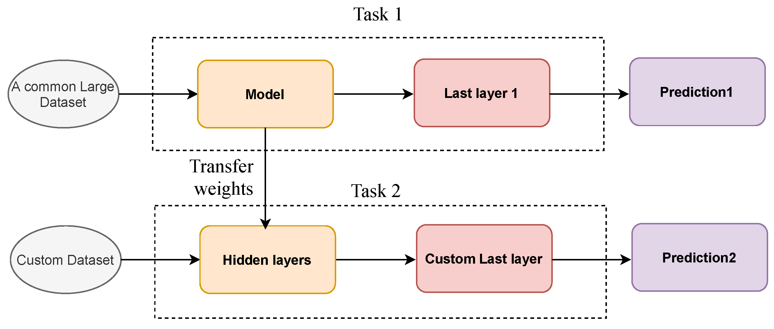
Barbedo [55] investigated how dataset size and diversity affect the performance of DL techniques applied to plant diseases. An image dataset of leaves with a small number of samples for the CNN model was used to investigate the behavior of GoogLeNet under different conditions. Data augmentation and transfer learning methods were used to train the CNN. The results showed that even with transfer learning and augmentation techniques, CNN requires a large number of images to extract useful features from the data. Even though a large number of images can be easily acquired with the new technology, labeling the dataset is time-consuming. One option proposed in this paper was to share the dataset, but as mentioned earlier, the two environments are not the same in agriculture. The effect of removing the background of the images on the accuracy of the model was also investigated. The model has trained again with the images without background. The model has trained again with the images without background. The results show different behaviors with respect to the accuracy of the model, including no significant effect, a significant improvement in accuracy in some cases, a significant decrease in accuracy, and mixed results (improved accuracy in some diseases while the error rate increased in others). From the significant decrease in accuracy for some plants, it was inferred that the CNN model sometimes uses the background of the model to classify the images. An attempt that can be made here is to train the model with both datasets (with and without background) and investigate the accuracy of the model in this case.

Ferentinos (2018) [63] used AlexNet, AlexNetOWTBn [64], GoogLeNet, Overfeat [10], and VGG models to identify 25 plant disease in 58 different classes of (plant, disease) combinations, including some healthy plants. The dataset used was images of healthy and infected leaves of the plants from the Plantvillag database (https://github.com/spMohanty/PlantVillage-Dataset, accessed on 17 November 2021). More than 37.3% of the images in the dataset were taken under real cultivation conditions in the field, and the other images were taken under laboratory conditions. In the first experiment, the number of images acquired under laboratory conditions and real conditions was kept similar in the training and test set, and the models were trained using this dataset. The VGG model performed best on the test set with an accuracy of 99.53%.

They also investigated the significance of the presence of field-captured images in the training set. From the 58 available classes of the form (plant, disease), the 12 that contained images of both types were selected. Two experiments were conducted with these 12 classes, and two CNN models were developed: one was trained with images under laboratory conditions and tested with images under field conditions, and another was trained with images under field conditions and tested with images under laboratory conditions. Although the number of images acquired under field conditions was less than the number of images acquired under laboratory conditions, the CNN model trained only with images under field conditions performed better with an accuracy of 68% than the CNN model trained only with images under laboratory conditions with an accuracy of 33%. This result shows the importance of the presence of the images acquired under field conditions. From the misclassification image, they point out some problematic situations, including images with extensive partial shading on the leaves, images with multiple objects in addition to the image, images where the leaf occupies a very small and non-centric part of the frame, and images without leaves.

Jiang et al. [65] implemented the CNN models to detect five common apple leaf diseases using images from the field. By applying data augmentation, such as rotational transformations, horizontal and vertical flips, intensity disturbances, and Gaussian noise, 26,377 disease images were generated. The problem with SDD is that it cannot detect a small object, and also, an object can be detected multiple times. To overcome these drawbacks, they developed an SSD model with a VGG-INCEP as the backbone, where two GoogLeNet inception layers replace two convolutional layers of the VGG model. Moreover, the structure of feature extraction and fusion is designed by applying the Rainbow concatenation method instead of the pyramid (which is used in the SSD model) to improve the performance of feature fusion. The results showed that the data augmentation improved the accuracy of the model by 6.91% compared to the original dataset. Moreover, the proposed model achieved the best performance compared to faster R -CNN and SSD with VGG and Rainbow SSD (RSSD) model.

To investigate the effect of using a deep model as a backbone, ResNet-101 was used as a feature extractor for SSD. The results show that ResNet-101 does not lead to any improvement. In terms of speed, Faster RNN was the slower model with more accuracy. The proposed model with 78.80% mAP and 23.13 Frames Per Second (FPS) was more accurate than SDD and RSSD, but SSD outperformed the other models in terms of time inference. By examining the misclassified images, it was indicated that similarity between diseases, misclassified background, and light condition were the challenges in classification.

Karthik et al. [66] proposed a Residual Attention Network for disease detection in tomato leaves. The main idea of attention is to focus on the relevant parts of the input to produce outputs. The dataset was collected from the open-source website Plantvillage and contained one healthy class and three diseases. They implemented three models. One was a traditional CNN model, the second used the three residual layers introduced into the CNN model as part of the ResNet architecture, and the last used an attention mechanism on top of the residual CNN for effective feature learning. The traditional CNN-based methods focus on ordered feature learning, starting from basic image-level features such as edges, color, etc., to complex texture-based differences [66]. In the deeper layer, some important features extracted in the first layer may be lost. The residual layers are designed to avoid this problem [66]. They concatenate the extracted features from the earlier layers with the deeper layers. In addition, the attention mechanism is used to extract the relevant parts of the feature maps. The Residual Attention Network CNN performed better with an overall accuracy of 98% than the Vanilla Residual Network with an accuracy of 95% and the traditional CNN model with an accuracy of 84%.

Liu et al. [67] implemented the model Cascade Inception to detect four common apple leaf diseases in images captured in the field. The Cascade Inception was a modified AlexNet model with inception layers from GoogleNet. Various data enhancement methods such as image rotation, mirror symmetry, brightness adjustment, and PCA jittering were applied to the training images. Moreover, the fully connected layers were replaced by convolutional layers, which results in fewer parameters and avoids overfitting. The proposed model was trained using the optimization method Nesterov Accelerated Gradient (NAG) and achieved an accuracy of 97.62%. The performance of the proposed model was compared with SVM and BP neural networks, standard AlexNet, GoogLeNet, ResNet-20, and VGGNet-16. Transfer learning method was used to train VGGNet-16 and achieved 96% accuracy. Standard AlexNet, GoogLeNet, and ResNet-20 were trained from scratch using SGD-optimization and achieved a maximum accuracy of 95.69%. The SVM and BP, which achieved an accuracy of less than 60%, show that the traditional approaches rely heavily on the expert developed classification features to improve the recognition accuracy. They also investigated the effect of data augmentation methods and optimization algorithms on accuracy. The model with the SGD optimizer achieved 93.32% accuracy, while the model with NAG achieved 97.62% accuracy. The data augmentation methods improved the performance of the model by 10.83%. The advantage of the model is that it outperformed other CNN models in terms of training time and memory required. Furthermore, the number of parameters of the model was less than AlexNet and GoogleNet. One point that emerges from the paper is that GoogleNet and AlexNet were trained using the SGD optimizer, and the proposed model was trained using the NAG method, but as mentioned in the paper, SGD has the “local optimum” problem. In addition, the models were not compared based on the inference time.

Table 1. Feature descriptions of recent published papers in the field of “Disease Detection”.

References	Application	Data Used	Model	Metric Used	Model Performance
Kerkech et al. [61]	Detect Esca disease in grapevine using UAV RGB images.	The images were collected using a UAV system with an RGB sensor.	A CNN model was trained with different combinations of patch sizes and different color spaces.	AC	The CNN model trained with the RGB and YUV color spaces has a better performance compared to the models trained with HSV and LAB. Moreover, The model was obtained by combining YUV and RGB trained with vegetation indices gave better performances than the models trained with YUV and RGB.
Kerkech et al. [62]	Segmentation of the plant symptomatic area	A Quadcopter drone with two camera sensors	SegNet	P, R, $F_1$, AC	The model trained with RGB images outperformed the model trained with infrared images.
Barbedo [55]	Disease detection on 12 plants with a variety of diseases.	The images were taken with a variety of digital cameras and mobile devices.	GoogleNet	AC	CNN’s AC using the original image as the dataset was 84% and using the removed background was 87%.
Ferentinos (2018) [63]	Identification of 25 plant disease in 58 different classes of (plant, disease).	https://github.com/spMohanty/PlantVillage-Dataset, accessed on 17 November 2021	AlexNet, AlexNetOWTBn, GoogLeNet, Overfeat, and VGG models	AC	The VGG model performed best on the test set. Furthermore, the CNN model trained only with images under field conditions performed better than the CNN model trained only with images under laboratory conditions.
Jiang et al. [65]	Identification of apple leaf diseases.	Images were taken in the field, and some of them were in the laboratory.	SSD with base VGG-INCEP.	mAP	SSD with VGG-INCEP as base achieved better performance with an mAP of 78.80% compared to FR-CCN and SSD with VGG and ResNet as the base.

Table 1. Feature descriptions of recent published papers in the field of “Disease Detection”.

References	Application	Data Used	Model	Metric Used	Model Performance
Kerkech et al. [61]	Detect Esca disease in grapevine using UAV RGB images.	The images were collected using a UAV system with an RGB sensor.	A CNN model was trained with different combinations of patch sizes and different color spaces.	AC	The CNN model trained with the RGB and YUV color spaces has a better performance compared to the models trained with HSV and LAB. Moreover, The model was obtained by combining YUV and RGB trained with vegetation indices gave better performances than the models trained with YUV and RGB.
Kerkech et al. [62]	Segmentation of the plant symptomatic area	A Quadcopter drone with two camera sensors	SegNet	P, R, $F_1$, AC	The model trained with RGB images outperformed the model trained with infrared images.
Barbedo [55]	Disease detection on 12 plants with a variety of diseases.	The images were taken with a variety of digital cameras and mobile devices.	GoogleNet	AC	CNN’s AC using the original image as the dataset was 84% and using the removed background was 87%.
Ferentinos (2018) [63]	Identification of 25 plant disease in 58 different classes of (plant, disease).	https://github.com/spMohanty/PlantVillage-Dataset, accessed on 17 November 2021	AlexNet, AlexNetOWTBn, GoogLeNet, Overfeat, and VGG models	AC	The VGG model performed best on the test set. Furthermore, the CNN model trained only with images under field conditions performed better than the CNN model trained only with images under laboratory conditions.
Jiang et al. [65]	Identification of apple leaf diseases.	Images were taken in the field, and some of them were in the laboratory.	SSD with base VGG-INCEP.	mAP	SSD with VGG-INCEP as base achieved better performance with an mAP of 78.80% compared to FR-CCN and SSD with VGG and ResNet as the base.

Ramcharan et al. [12] trained the SSD object detection model to identify three diseases, two types of pest damage, and nutrient deficiency in cassava at the mild and pronounced stages. A dataset was collected from the field, which was divided into 80–20 as training and testing sets. The model achieved 94 ± 5.7% mAP on the test dataset. The trained model was used on a mobile phone to investigate the performance of the model in the real world. One hundred twenty images of leaves were captured using a mobile device of the study experiment, and the model inference was run on a desktop and mobile phone to calculate the performance metrics of the trained model. The results show that the average precision of the model on the real dataset decreases by almost 5%, but the average recall decreases by almost half, and the $F_1$-score decreases by 32%. Furthermore, the results show that the model performs better on the leaves with pronounced symptoms than on the leaves where the symptoms are only mildly pronounced.

Picon et al. [68] used DL model to detect seventeen diseases of five crops (wheat, barley, corn, rice, and rapeseed) in images captured in the field. The dataset contained several challenges, such as multiple diseases on the same plant, similar visual symptoms among diseases, images of early and early-stage diseases, and diseases of leaves, and stems. To improve the accuracy of the model, the crop ID was used in the network. The crop ID was defined as a categorical vector with K components, where K is the number of crops in the model. Several models were trained. The first approach was to train an independent model for each crop and the second approach was to train a single model for the entire dataset. The results show that the multi-crop model had a similar performance to splitting the training dataset into the different crops (1% increased accuracy). However, the class of diseases with fewer images in the training set may benefit from the multi-crop model. The second approach was to add the crop ID to the multi-crop model. The results show that by adding crop id, the model can still benefit from more images for training, while crop ID information helps the network to discriminate between similar diseases.

Chen et al. [69] used pre-trained MobileNet V2 networks to identify twelve rice plant diseases. The dataset was collected from online sources and real agricultural fields. An attention mechanism was added to the model, and transfer learning was performed twice during model training to achieve better performance. The MobileNet-V2 achieved 94.12% accuracy on the PlantVillage dataset, while the MobileNet-V2 with attention and transfer learning achieved 98.26%. The five CNNs such as MobileNetv1, MobileNet-V2, NASNetMobile, EfficientNet-B0, and DenseNet121 were selected for comparison with the proposed models. In addition, two other networks named MobileNetv2-2stage and MobileAtten-alpha were trained. In the MobileNetv2-2stage model, transfer learning was performed twice to identify the images of plant diseases.

Similarly, in MobileAtten-alpha, the attention method was used instead of transfer learning twice. The proposed model (using attention and transfer learning twice) achieved the the second best accuracy of 98.84%. The DenseNet121 with an accuracy of 98.93% outperformed other models. MobileNetv2-2stage and MobileAtten-alpha achieved an accuracy of 98.68% and 96.80%, respectively. The proposed model was trained with images from the field and achieved an accuracy of 89.78%.

Table 2. Feature descriptions of recent published papers in the field of “Disease Detection”.

References	Application	Data Used	Model	Metric Used	Model Performance
Karthik et al. [66]	Identifying the type of infection in tomato leaves.	Plant Village Dataset.	Residual CNN with attention.	AC	Residual CNN with attention with an AC of 98% achieved better performance compared to CNN and residual CNN.
Liu et al. [67]	Identification of 4 apple leaves diseases.	Images were taken in field using digital color camera.	CNN (AlexNet+ +Inception layers from GoogleNet).	AC	Their model with an AC of 97.62% performed better than GoogLeNet, ResNet-20, VGGNet16, SVM, and BP, AlexNet.
Ramcharan et al. [12]	Identification of cassava pests and diseases.	Dataset from [70]	SSD	$F_1$-score	The $F_1$-score decreased by 32% when moving from the test set to real images.
Picon et al. [68]	Identification of 17 diseases and five crops by adding metadata to the model.	Images were taken by cell phone in real field wild conditions.	CNN (ResNet50	AC, $R^2$, Negative and positive predictive value	Adding plants species information to the model by concatenating plant information in the embedding layer improved the performance of the model (AC = 0.98)
Chen et al. [69]	Identify rice plant diseases from collected real-life images.	Online sources and agricultural fields.	MobileNet-V1, MobileNet-V2, DenseNet-121, NASNetMobile, EfficientNet-B0, proposed model.	AC, R, P, $F_1$-score	The proposed model with an accuracy of 0.98 out- performed the other models.

Table 2. Feature descriptions of recent published papers in the field of “Disease Detection”.

References	Application	Data Used	Model	Metric Used	Model Performance
Karthik et al. [66]	Identifying the type of infection in tomato leaves.	Plant Village Dataset.	Residual CNN with attention.	AC	Residual CNN with attention with an AC of 98% achieved better performance compared to CNN and residual CNN.
Liu et al. [67]	Identification of 4 apple leaves diseases.	Images were taken in field using digital color camera.	CNN (AlexNet+ +Inception layers from GoogleNet).	AC	Their model with an AC of 97.62% performed better than GoogLeNet, ResNet-20, VGGNet16, SVM, and BP, AlexNet.
Ramcharan et al. [12]	Identification of cassava pests and diseases.	Dataset from [70]	SSD	$F_1$-score	The $F_1$-score decreased by 32% when moving from the test set to real images.
Picon et al. [68]	Identification of 17 diseases and five crops by adding metadata to the model.	Images were taken by cell phone in real field wild conditions.	CNN (ResNet50	AC, $R^2$, Negative and positive predictive value	Adding plants species information to the model by concatenating plant information in the embedding layer improved the performance of the model (AC = 0.98)
Chen et al. [69]	Identify rice plant diseases from collected real-life images.	Online sources and agricultural fields.	MobileNet-V1, MobileNet-V2, DenseNet-121, NASNetMobile, EfficientNet-B0, proposed model.	AC, R, P, $F_1$-score	The proposed model with an accuracy of 0.98 out- performed the other models.

3.8.2. Fruit Detection and Yield Forecast

Yield forecasting is one of the most important and popular topics in precision agriculture because it is the basis for yield mapping and estimation, supply and demand matching, and crop and harvest management [8]. Modern approaches go far beyond simple forecasting based on historical data but incorporate methods from DL to provide a comprehensive multidimensional analysis of crop, climatic and economic conditions to maximize yields.

Silver and Monga [71] trained five CNN models to estimate grape yield from RGB images taken in a vineyard on harvest day using the camera of a Samsung Galaxy S3. The images of 40 grapevines were split into two parts, one for the left cordon and one for the right cordon, resulting in a total of 80 cordons. A simple CNN was trained by inputting the RGB images of the left and right cordons and estimating the grape yield. The second model was the same as the first model, but the input to the model was the right cordon images and the inversion of the left cordon images to look similar to right cordon images. The third model, an autoencoder network, is trained to a high level of accuracy and the CNN encoder weights are transferred as starting weights into the CNN model for the yield estimation model. In the fourth model, an autoencoder model was trained to output the density map of the grapes in the image. Then, the weights of the encoder are transferred as initial parameters into the CNN model for yield estimation. The last model was trained with the output of the autoencoder for the density map as input to the CNN model for yield estimation instead of the RGB images. The CNN models with flipped images outperformed the simple CNN model with an MAE % of 15.43. The models of transfer learning from Density Map Network Representation with MAE % of 11.79 achieved the best performance among the other models. The last model with MAE % of 15.99 did not perform as well as the fourth model because the accuracy of the density map estimates was quite low. The results show that transfer learning, when used properly, can improve recognition accuracy.

Aguiar et al. [72] trained SSD MobilenetV1 and the Inception model to detect Grape Bunch in Mid Stage and early stages and then transferred the trained model to the TPU-Edge device to investigate the temporal accuracy of the model. The same strategy in [18] was used to collect the dataset and it is publicly available (https://doi.org/10.5281/zenodo.5114142, accessed on 3 November 2021) with 1929 vineyard images and their annotation. Overall, SSD MobileNet-V1 performed better than the Inception model, as it had a higher F_1 score, AP, and mAP. The early stage was more difficult to detect than the middle growth stage. The first class represented smaller clusters that were more similar in color and texture to the surrounding foliage, making them more difficult to detect. SSD MobileNet-V1 showed an AP of 40.38% in detecting clusters at an early growth stage and 49.48% at a medium growth stage. In terms of time, SSD MobileNet-V1 was more than four times faster than the Inception model on TPU-Edge Device.

Ghiani et al. [31] used Mask R-CNN with ResNet101 as a backbone which was pre-trained with the dataset COCO (https://cocodataset.org/#home, accessed on 18 November 2021) for detecting grape branches on the tree. An open-source dataset GrapeCS-ML [73] containing more than 2000 images without annotation of fifteen grape varieties at different stages of development in three Australian vineyards was used to train the model. In addition to the GrapeCS-ML dataset, 400 images were collected from the island of Sardinia (Italy). The result obtained by applying the detector to the test samples was an mAP value of 92.78%. To investigate the generalizability of the proposed model, the model trained on the GrapeCS-ML dataset was tested on its internal dataset. The dataset contained different grape varieties, vegetation, and colors than the GrapeCS-ML dataset. An mAP of 89.90% was obtained with the internal dataset, indicating that the model can be used in other fields. To investigate the significance of the size of the dataset used for training and the importance of the augmentation techniques, the size of the original dataset was reduced to 10% of the training images in one case with augmentation and the other case without augmentation of the dataset. The mAP was reduced by up to 5%, especially in the experiments performed without augmentation. It was observed that the recognition accuracy decreased for images with overlap between clusters.

In Milella et al. [74], a system for the automatic estimation of harvest volume and for detecting grapes in vineyards using an RGB-D sensor on board an agricultural vehicle has been proposed. An RGB-D sensor is a special type of depth detection device that works in conjunction with an RGB camera and is able to add depth information to the conventional image pixel by pixel. The approach to determine the crop volume involved three steps: the 3D reconstruction of the vine rows, the segmentation of the vines using a deep learning method, and the estimation of the volume of each plant. In the first step, the depth output from the camera was not used because the parameters of the algorithm are fixed and cannot be configured. Instead, the semi Global Matching (SGM) algorithm was used, which is a computer vision algorithm for estimating a dense disparity map from a rectified stereo image pair. A box-grid filter is then used to merge the point clouds.

In segmentation, a segmentation algorithm was first used to separate the canopy from the background using the green–red vegetation index (GRVI), and then k-means were used to identify each plant. Based on the results of the clustering algorithm, different plants were calculated and an estimate of the volume per plant was performed. Finally, the pre-trained AlexNet, VGG16 and VGG19, and GoogLeNet were trained to perform grape cluster detection in 5 different classes (grapes, vineyard stakes, vine stems, cordons, canes, leaves, and background). The VGG model performed the best with an accuracy of 91.52.

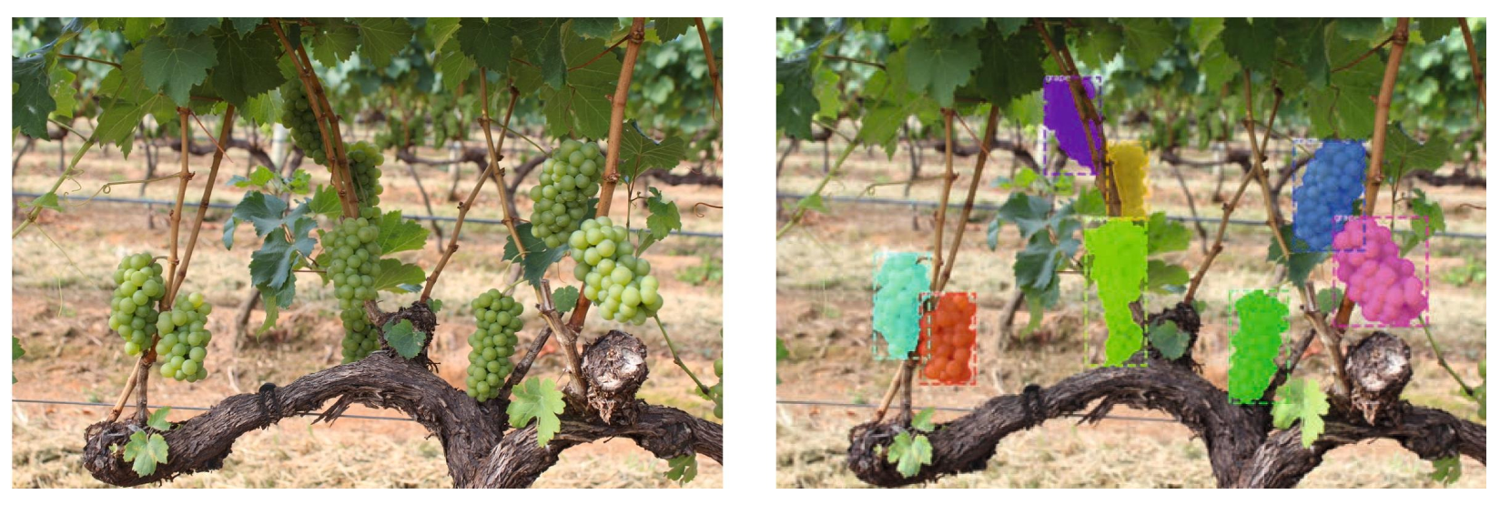
Santos et al. [26] used deep learning models and computer vision models to estimate grape wine yield from RGB images. Images were captured with a Canon EOS REBEL T3i DSLR camera and a Motorola Z2 Play smartphone from five different grape varieties. The dataset named Embrapa Wine Grape Instance Segmentation Dataset (WGISD) with 300 RGB images is publicly available (https://doi.org/10.5281/zenodo3361736, accessed on 18 November 2021). Models from DL such as Mask R-CNN, YOLOv2, and YOLOv3 were trained to detect and segment grapes in the images. Then, an image processing algorithm called Structure-from-Motion (SfM) was used to perform spatial registration, integrating the data generated by the CNN-based step. In the final step, the results of the CV model were used to remove the clusters detected in different images to avoid counting the same clusters in several images. The Mask R-CNN with ResNet101 as the backbone outperformed YOLOv2 and YOLOv3 in terms of object detection, but the YOLO model outperformed the Mask R-CNN in terms of detection time. The worst performance was obtained with YOLOv3. To verify the performance of Mask R-CNN+SfM, 500 key-frames of a video were used, and the result is shown in a video at https://youtu.be/1Hji3GS4mm4, accessed on 17 November 2021.

Palacios et al. [75] applied the method of deep learning to detect the flowering of the vine and used it for the estimation of early yield estimation. Images of six grapevine varieties were acquired using a mobile platform developed at the University of La Rioja. The RGB camera was a Canon EOS 5D Mark IV RGB with a full-frame CMOS sensor. The ground truth was acquired using the algorithm in [76]. This algorithm was developed to process only images with a single inflorescence and a dark background. In the first step, SegNet was used with VGG (VGG16 and VGG19) as a backbone to segment and extract the inflorescences contained in the images. Then, these regions were used to count the flowers in each inflorescence using three algorithms, including SegNet, Watershed Flower Segmentation, and a linear model. The SegNet with VGG19 as backbone outperformed the model with VGG16 in terms of IOU and $F_1$-score. For flower recognition, the SegNet model with VGG19 was trained to classify a group of flowers per image into three classes including contour, center, and background. After segmentation, false-positive filtering of flower segmentation was performed. Here, the flowers whose center and contour was segmented, and whose contour surrounded the center above a certain threshold were considered as true positives. The $F_1$-score reached its highest value when contour filtering was set to 50%, resulting in an $F_1$-score of 0.729. The best $F_1$-score for the watershed approach was 0.708 and the worst performance in counting flowers was obtained with linear regression in the form of the Root Mean Square metric. The number of flowers counted using SegNet-VGG19 for inflorescence extraction and flower detection, and flower counting using the algorithm of [76] showed a correlation with $R^2$ close to or above 0.75 for all cultivars.

Table 3. Feature descriptions of recent published papers in the field of “Fruit detection and Yield estimation”.

References	Application	Data Used	Model	Metric Used	Model Performance
Silver and Monga [71]	Estimate grape yield from RGB images.	Images were taken in of a vineyard on harvest day using the camera of a Samsung Galaxy S3.	Five CNN models from scratch trained with five different techniques for training	MAE	The models of transfer learning from Density Map Network Representation. with MAE% of 11.79 achieved the best performance among the other models.
Aguiar et al. [72]	Detect Grape Bunch in Mide Stage and early stages.	The images were acquired from four different vineyards in Portugal.	SSD Inception-V2, SSD MobileNet- V1	IOU, mAP, R	The SSD Inception-V2 had higher precision than the SSD MobileNet-V1 at all confidence values, but lower recall. In terms of time, SSD MobileNet-V1 was more than four times faster than the Inception
Ghiani et al. [31]	Detecting grape branches in the tree	GrapeCS-ML [73] and 400 images were collected from field	Mask R-CNN with ResNet101 as back- bone	IOU, mAP	The model achieved an mAP value of 92.78%
In Milella et al. [74]	Estimation of harvest volume and for detecting grapes in vine-yards	Images was collected from field using RGB-D sensor	AlexNet, VGG, GoogleNet	P, R, AC, TP (true positive)	The VGG model performed the best with an accuracy of 91.52%.
Santos et al. [26]	Estimate grape wine yield from RGB images.	Images were captured with a camera from five different grape varieties.	Mask R-CNN and YOLOv2 and YOLOv3	P, R, $F_1$-score	The Mask R-CNN with ResNet 101 as the back-bone outperformed YOLOv2 and YOLOv3 in terms of object detection, but the YOLO model outperformed the Mask R-CNN in terms of detection time.
Palacios et al. [75]	Detect the flowering of the vine, and used it for the estimation of early yield estimation	Images of six grapevine varieties were acquired using a mobile platform	SegNet model with VGG19	IOU and $F_1$-Score	The number of flowers counted using SegNet- VGG19, and flower counting using the algorithm of [76] showed a correlation with R2 close to or above 0.75 for all cultivars.

Table 3. Feature descriptions of recent published papers in the field of “Fruit detection and Yield estimation”.

References	Application	Data Used	Model	Metric Used	Model Performance
Silver and Monga [71]	Estimate grape yield from RGB images.	Images were taken in of a vineyard on harvest day using the camera of a Samsung Galaxy S3.	Five CNN models from scratch trained with five different techniques for training	MAE	The models of transfer learning from Density Map Network Representation. with MAE% of 11.79 achieved the best performance among the other models.
Aguiar et al. [72]	Detect Grape Bunch in Mide Stage and early stages.	The images were acquired from four different vineyards in Portugal.	SSD Inception-V2, SSD MobileNet- V1	IOU, mAP, R	The SSD Inception-V2 had higher precision than the SSD MobileNet-V1 at all confidence values, but lower recall. In terms of time, SSD MobileNet-V1 was more than four times faster than the Inception
Ghiani et al. [31]	Detecting grape branches in the tree	GrapeCS-ML [73] and 400 images were collected from field	Mask R-CNN with ResNet101 as back- bone	IOU, mAP	The model achieved an mAP value of 92.78%
In Milella et al. [74]	Estimation of harvest volume and for detecting grapes in vine-yards	Images was collected from field using RGB-D sensor	AlexNet, VGG, GoogleNet	P, R, AC, TP (true positive)	The VGG model performed the best with an accuracy of 91.52%.
Santos et al. [26]	Estimate grape wine yield from RGB images.	Images were captured with a camera from five different grape varieties.	Mask R-CNN and YOLOv2 and YOLOv3	P, R, $F_1$-score	The Mask R-CNN with ResNet 101 as the back-bone outperformed YOLOv2 and YOLOv3 in terms of object detection, but the YOLO model outperformed the Mask R-CNN in terms of detection time.
Palacios et al. [75]	Detect the flowering of the vine, and used it for the estimation of early yield estimation	Images of six grapevine varieties were acquired using a mobile platform	SegNet model with VGG19	IOU and $F_1$-Score	The number of flowers counted using SegNet- VGG19, and flower counting using the algorithm of [76] showed a correlation with R2 close to or above 0.75 for all cultivars.

Kang and Chen [34] implemented DaSNet-v2, which is an ’Encoder–Decoder with atrous convolution developed in Deeplab-v3+ to detect and segment the apple in an orchard for harvesting by a robot. Atrous convolution is a type of convolutional layer that allows control of the resolution of the features computed by the CNN. The dataset was collected from an apple orchard as RGB-D and RGB. The RGB-D was used to visualize the environment. A lightweight model, Resnet 18, was used as the backbone of the DaNet-v2 to ensure its deployment on the Jetson-TX2 with limited computing capacity. In addition, the model was trained with the Resnet50 and Resnet101 backbones. The performance of the model with the Resnet101 backbone was compared with DaSNet-v1, YOLO-v3, faster-RCNN, and the Mask-RCNN. DaSNet-v2 and Mask-RCNN with $F_1$-score of 0.873 and 0.868, respectively, outperformed the other models. However, DaSNet-v2 outperformed mask-RCNN with a computational efficiency between 306 and 436 ms with a time of 1.3 s. The results also show that single-stage detection models such as Yolo have better computational efficiency compared to two-stage detectors. The model was implemented on Jetson-TX2, a lightweight backbone of Resnet-18, and the experimental results show that DaSNet-v2 with Resnet-18 can achieve similar performance in recall and precision of detection compared to YOLO-v3. Environmental factors such as strong sunlight reflection, shadows, and appearance variations of fruits in color, shape, occlusion, or viewing angle could lead to false-negative detection results. RGB-D images were processed using DaSNet-v2 and the PPTK toolbox, a Python package for image visualization, to deploy the robot in the orchard.

Koirala et al. [77] developed a DL model, called Mango-YOLO, based on YOLO-v3 and YOLO-v2 (tiny) for counting mangoes on trees. YOLOv2 (tiny) has a small architecture with only nine convolutional layers, six pooling layers, and one detection layer, sacrificing accuracy for speed. YOLOv3 [22] is based on Darknet-53 and improves upon YOLOv2 [78]. The Mango YOLO had 33 layers compared to 106 layers in YOLO-v3 and 16 layers in YOLO-v2 (tiny). The reduction in the number of layers is expected to reduce computation time and detect mangoes more accurately. The model was trained on the dataset collected from five orchards. The Mango-YOLO achieved better performance with an accuracy of 0.967% compared to YOLO-v2 (tiny) (0.9% ) and YOLO-v3 (0.951%). In terms of time inference, the Mango YOLO with 15 ms was faster than YOLO-v3 (25 ms) and slower than YOLO-v2 (tiny) (10 ms). Moreover, Mango-YOLO was trained once from scratch on the augmented dataset, and the second time transfer learning was used using the COCO dataset. The models had the same performance on the test set, and the reason was explained by the fact that the COCO dataset does not contain Mango images. The false detection over images taken with Canon camera shows resizing of the images and results in image distortion with leaves taking a curved shape resembling the fruit and overexposed areas on branches, trunks, and leaves.

Liang et al. [79] applied the SSD network to detect mango and almond on tree fruits. The dataset in [80] was used to train the model. The SSD model used the original and sampled a patch such that the minimum Jaccard overlap with the objects is 0.1, 0.3, 0.5, 0.7, or 0.9, and finally randomly sampled the input image. The size of each sampled area and the minimum Jaccard overlap are critical for object detection. These two parameters were changed to adopt the SSD model for small mango detection. Using VGG16 as the basic framework for the SDD outperformed the SSD with ZFNet. Furthermore, using the input image size of $400\times 400$ and $500\times 500$ as the input of the model, the model achieved better performance than SSD with an input size of $300\times 300$. The model outperformed the faster RCNN in terms of speed and accuracy. The challenges related to mango detection on the tree were considered in the paper: the size of mango on the whole image, blocking the mango with leaves, branches, resizing the original image, making mango smaller, and similarity between mango and background.

Tian et al. [81] developed YOLO-V3 with DenseNet as the backbone to detect apples on trees. They used two datasets for training. The first one contained images of apples at one growth stage, and the second one contained images taken at different growth stages. The model showed better performance for mature apples than for young and growing apples because the color features were more prominent, the individual volume was larger, and there was less overlap. The results also showed that the $F_1$-score of the model trained with the first dataset was higher than that of the model trained with the second dataset. The performance of the trained model decreased for images with partial occlusion of apples with branches and leaves but is still an acceptable result (IOU = 0.889 for mature apples ).

The model achieved the best performance compared to Faster R-CNN, YOLOV2, and the original YOLOv3. In terms of time inference, the model was faster than Faster R-CNN and similar to YOLOv3. The $F_1$-score and IOU of the model without data augmentation methods decreased by 0.033 and 0.058, respectively.

Zhou et al. [82] implemented an SSD model with two lightweight backbones MobileNetV2 and InceptionV3, to develop an Android APP called KiwiDetector that detects kiwis in the field. Quantization is a technique for performing computations and storing tensors with bit widths smaller than floating-point numbers. When training a neural network, 32-bit floating-point weights and activation values are typically used. A quantized model performs some or all operations with tensors using integers instead of floating-point values. This allows the computational complexity to be reduced and the trained model can be used on devices with lower resource requirements. The quantization method was used to compress the model size and improve the detection speed by quantizing the weight tensor and activation function data of convolutional neural networks from 32 to bit floating-point numbers to an 8-bit integer. The results showed that MobileNetV2, quantized MobileNetV2, InceptionV3, and quantized InceptionV3 achieve a true detection rate of 90.8%, 89.7%, 87.6%, and 72.8%, respectively. The quantized MobileNetV2 on the Huawei P20 smartphone outperformed the other models in terms of detection speed (103 ms/frame) and size. Although the SSD with MobileNetV2 was more accurate than the SSD with quantized MobileNetV2, the SSD with quantized MobileNetV2 was 37% faster. The problem with kiwi detection was that overlapping kiwis were reported, which the model counts as one kiwi.

3.8.3. Weed Detection

Besides disease, weeds are considered to be a prevalent threat to agricultural production. These are plants considered undesirable in a particular situation, as they may compete with crops for sunlight and water, resulting in crop and economic loss. One significant problem in weed control is that they are difficult to detect and distinguish from crops [8]. DL algorithms can improve weed detection and discrimination at a lower cost with reduced environmental problems and side effects. These technologies could power robots that detect and remove weeds.

Bah et al. [83] proposed a CNN model with unsupervised training dataset annotation collection for weed detection in UAV images of bean and spinach fields. They assumed that crops are grown in regular rows and that plants growing between the rows are considered weeds. The Hough transform was applied to the skeleton to detect the rate of plant rows, and then a simple linear iterative clustering (SLIC) algorithm was applied to create a marker and delineate the plant rows. This algorithm generated superpixels based on k-mean clustering. After row detection, a blob coloring algorithm was used to identify the weeds. The unsupervised training dataset was used to train ResNet18 for weed detection in the images. The supervised learning method performed 6% better than the unsupervised learning method in the bean field and about 1.5% better in the spinach field. The low number of weeds between rows may explain the difference in performance in the bean field. The performance of the model was compared with SVM and RF. In general, ResNet18 shows better performance in supervised and unsupervised learning methods than SVM and RF.

Table 4. Feature descriptions of recent published papers in the field of “Fruit detection and Yield estimation”.

References	Application	Data Used	Model	Metric Used	Model Performance
Kang and Chen [34]	Counting apple on tree.	The images were taken in the field with a camera.	C-RCNN+LedNet with a light-weight (LW) as backbone, resnet-50, resnet-101, darknet-53.	IOU, P, R, $F_1$-score	LedNet with resnet-101 achieved an AC of 0.864 and LedNetwith LW achieved an Ac of 0.853.
Koirala et al. [77]	Counting mango on trees.	The images were taken in the field.	CNN (Mango-YOLO)	$F_1$-score	Mango-YOLO with an $F_1$-score of 0.97 achieved better performance compared to faster R-CNN, SSD, and YOLO.
Liang et al. [79]	Detection of mango and almond fruits on the tree.	https://arxiv.org/abs/1610.03677, accessed on 15 November 20221	SSD with VGG-16 and ZFNet	IOU, $F_1$-score	The model outperformed the faster RCNN in terms of speed and accuracy.
Tian et al. [81]	Detection of apple in image and yield estimation.	Image capture was performed with a camera in the field.	Improved YOLO-V3 with DenseNet as the backbone.	$F_1$-score	The proposed model with an $F_1$-score of 0.817 had better performance compared to YOLO-V2, YOLOV3, and Faster R-CNN.
Zhou et al. [82]	Detection of kiwi fruit in the orchard with android smartphones.	Collected from the orchard.	MobilNetV2, quantized MobileNetV2, InceptionV3, quantized InceptionV3.	IOU, TDR, FDR	Quantized MobileNetV2 outperformed the other models in terms of accuracy, speed, and size.

Table 4. Feature descriptions of recent published papers in the field of “Fruit detection and Yield estimation”.

References	Application	Data Used	Model	Metric Used	Model Performance
Kang and Chen [34]	Counting apple on tree.	The images were taken in the field with a camera.	C-RCNN+LedNet with a light-weight (LW) as backbone, resnet-50, resnet-101, darknet-53.	IOU, P, R, $F_1$-score	LedNet with resnet-101 achieved an AC of 0.864 and LedNetwith LW achieved an Ac of 0.853.
Koirala et al. [77]	Counting mango on trees.	The images were taken in the field.	CNN (Mango-YOLO)	$F_1$-score	Mango-YOLO with an $F_1$-score of 0.97 achieved better performance compared to faster R-CNN, SSD, and YOLO.
Liang et al. [79]	Detection of mango and almond fruits on the tree.	https://arxiv.org/abs/1610.03677, accessed on 15 November 20221	SSD with VGG-16 and ZFNet	IOU, $F_1$-score	The model outperformed the faster RCNN in terms of speed and accuracy.
Tian et al. [81]	Detection of apple in image and yield estimation.	Image capture was performed with a camera in the field.	Improved YOLO-V3 with DenseNet as the backbone.	$F_1$-score	The proposed model with an $F_1$-score of 0.817 had better performance compared to YOLO-V2, YOLOV3, and Faster R-CNN.
Zhou et al. [82]	Detection of kiwi fruit in the orchard with android smartphones.	Collected from the orchard.	MobilNetV2, quantized MobileNetV2, InceptionV3, quantized InceptionV3.	IOU, TDR, FDR	Quantized MobileNetV2 outperformed the other models in terms of accuracy, speed, and size.

Ferreira et al. [36] implemented the unsupervised learning models JULE and DeepCluster to detect weeds in the field. The JULE consists of stacked multiple combinations of convolutional layer, batch normalization layer, ReLU layer, and pooling layer. AlexNet and VGG16 were implemented as the basis of the DeepCluster model to extract features, and then K-means is used as the clustering algorithm. Two datasets, Grass-Broadleaf [84] and DeepWeeds [85] were used in this work. The DeepCluster model performed better than the JULE model on both datasets with a large number of clusters. The DeepCluster with a base of Alexnet and VGG achieved similar performance, with Alexnet performing better on DeepWeed and VGG on the other dataset. To investigate the effect of transfer learning on unsupervised learning, the pre-trained VGG and AlexNet were used on ImageNet. The pre-trained model did not improve the accuracy of Grass-Broadleaf, but it did improve the accuracy of DeepWeed. The data augmentation also improved the accuracy of the unsupervised learning methods. They also used semi-supervised data labeling. Semi-supervised learning is a machine learning approach that deals with the use of labeled and unlabeled data. In the semi-supervised method, labeled images from the DeepCluster model were used to train Inception-V3, VGG, and ResNet. Inception-V3 and VGG outperformed ResNet on the Grass-Broadleaf and DeepWeeds dataset, respectively.

Milioto et al. [86] modified Encoder–Decoder CNN architecture in [87] to distinguish weeds from crops and soil. The number of convolutional layers was decreased to reduce time inference, and additional vegetation indices (14 channels) were included in the input for more accurate detection. The dataset of three fields was used. Three networks were trained with different inputs: one with RGB images, another with RGB and near-infrared (NIR) images, and the last one was trained with 14 channels such as RGB, Excess Green (ExG), Excess Red (ExR), color index of Vegetation Extraction (CIVE), and Normalized Difference Index (NDI). To investigate the generalization ability of the proposed model, the model was trained on the images of one field and tested on images of all fields. The results indicate that feeding these 14-channels into the input can speed up the training and improve the performance of the model on the unseen dataset compared to the model trained on RGB images and RGB+NRI but still, the recall and precision of the model on the unseen field drop sharply (11–50%).

Another experience was conducted to investigate the generalization capacity of the proposed model. The trained model was retrained on the unseen dataset with 10, 20, 50, or 100 images in the training set. The performance of the RGB network when retrained with 100 images is almost the same as the performance of the proposed model trained with ten images. The inference time of the proposed model on PC and Jetson TX2 platform was also found to be 44 ms and 210 ms, respectively, which is slower than the model trained with RGB images with 31 ms and 190 ms, respectively.

Lottes et al. [30] developed an encoder–decoder Fully Convolutional Network (FCN) with the sequential model for weed detection in sugar beet fields. The encoder–decoder FCN was used to extract features from the input images, and the sequential model processed the five images in a sequence using 3D convolution and output a sequence code that was used to learn sequential information about the weeds in five images in a sequence. The results showed that the encoder-decoder with a sequential model improved the $F_1$-score of the module by almost 11–14% compared to the encoder-decoder FCN. The results indicated that the changes in the visual appearance of the images in the training and test dataset could lead to a decrease in model performance, and adding additional information, such as vegetation indices, leads to better generalization for other fields.

Wang et al. [88] used the encoder–decoder with Atrous Convolution for pixel-wise semantic segmentation of crops and weeds. The two datasets for sugar beet and oilseed included in the paper were taken under completely different lighting conditions. To mitigate the effects of the different lighting conditions, three image enhancement methods were evaluated, including Histogram Equalization (HE), Auto Contrast, and Deep Photo Enhancer. The models were also trained with various inputs, including YCrCb and YCgCb color spaces and vegetation indices such as Normalized Difference Index (NDI), Normalized Difference Vegetation Index (NDVI), Excess Green (ExG), Excess Red (ExR), Excess Green minus Excess Red (ExGR), Color Index of Vegetation (CIVE), Vegetative Index (VEG), and Modified Excess Green Index (MExG), Combined Indices (COM1), and COM2. For the sugar beet dataset, the model trained with NIR images enhanced by Auto Contrast outperformed the other models with a mean IOU of 87.13%. For the Oilseeds dataset, the models were trained with RGB images only, and the model trained with images enhanced by Deep Photo Enhancer outperformed the other models (mIOU = 88.91%). Moreover, the auto-contrast method outperforms other methods in terms of time inference.

Table 5. Feature descriptions of recent published papers in the field of “Weed Detection”.

References	Application	Data Used	Model	Metric Used	Model Performance
Bah et al. [83]	Weed detection in bean and spinach fields.	The images were taken with a DJI Phantom 3 Pro drone.	Simple linear iterative clustering (unsupervised)+ CNN (Resnet18)	AC	CNN trained with unsupervised labeling achieved an AC of 88.73 (spinach) and 94.34 (bean), and with supervised labeling achieved an AC of 94.84 (spinach) and 95.70 (bean).
Ferreira et al. [36]	Identification of weeds with unsupervised clustering.	The Grass-Broadleaf Dataset in [84] and DeepWeed in [85].	JULE, DeepCluster	AC, NMI	DeepCluster achieved better performance than JULE.
Milioto et al. [86]	Identification of weeds (additional vegetation indices added to the input).	Data was taken with a 4-channel RGB+NIR camera.	Mask R-CNN.	IOU, mIOU	The model achieved better performance by adding an extra channel at the input of the model (IOU = 80.8%)
Lottes et al. [30]	Crop and weed detection in the sugar field.	Dataset was taken with robots equipped with a 4-channel with RGB+NIR camera	Encoder–Decoder FCN (FC-DenseNet) sequential model.	Average $F_1$-score	The proposed model achieved better performance with a $F_1$-score of 92.3 compared to encoder-decoder FCN without a sequential model, random forests, and vanilla FCN.
Wang et al. [88]	Pixel-wise segmentation of field images into soil, crop, and weeds.	Two datasets used: the first Dataset in [89] and oilseed image acquired in the field	Encoder-decoder CNN with different inputs.	AC, IOU	The model with RGB input with an AC of 96.06 on dataset1 and 96.12 on dataset2 achieved the best performance. Image enhancement improved the results.

Table 5. Feature descriptions of recent published papers in the field of “Weed Detection”.

References	Application	Data Used	Model	Metric Used	Model Performance
Bah et al. [83]	Weed detection in bean and spinach fields.	The images were taken with a DJI Phantom 3 Pro drone.	Simple linear iterative clustering (unsupervised)+ CNN (Resnet18)	AC	CNN trained with unsupervised labeling achieved an AC of 88.73 (spinach) and 94.34 (bean), and with supervised labeling achieved an AC of 94.84 (spinach) and 95.70 (bean).
Ferreira et al. [36]	Identification of weeds with unsupervised clustering.	The Grass-Broadleaf Dataset in [84] and DeepWeed in [85].	JULE, DeepCluster	AC, NMI	DeepCluster achieved better performance than JULE.
Milioto et al. [86]	Identification of weeds (additional vegetation indices added to the input).	Data was taken with a 4-channel RGB+NIR camera.	Mask R-CNN.	IOU, mIOU	The model achieved better performance by adding an extra channel at the input of the model (IOU = 80.8%)
Lottes et al. [30]	Crop and weed detection in the sugar field.	Dataset was taken with robots equipped with a 4-channel with RGB+NIR camera	Encoder–Decoder FCN (FC-DenseNet) sequential model.	Average $F_1$-score	The proposed model achieved better performance with a $F_1$-score of 92.3 compared to encoder-decoder FCN without a sequential model, random forests, and vanilla FCN.
Wang et al. [88]	Pixel-wise segmentation of field images into soil, crop, and weeds.	Two datasets used: the first Dataset in [89] and oilseed image acquired in the field	Encoder-decoder CNN with different inputs.	AC, IOU	The model with RGB input with an AC of 96.06 on dataset1 and 96.12 on dataset2 achieved the best performance. Image enhancement improved the results.

3.8.4. Species Recognition

The classification of species (e.g., insects, birds, and plants) is another critical aspect of agricultural management. The traditional human approach to species classification requires specialists in the field and is time-consuming. Deep learning can provide more accurate and faster results by analyzing real-world data.

Rußwurm and Körner [90] trained LSTM and GRU models for multitemporal classification, which achieved high accuracy in crop classification tasks for many crops. Images were collected from SENTINEL 2A images between 31 December 2015 and 30 September 2016. For consistency with the LANDSAT series, the blue, green, red, near-infrared, and shortwave infrared 1 and 2 bands were selected for this assessment. The performance of the LSTM model was compared to the RNNs, the CNN model, and a baseline SVM. The LSTM model outperformed the other models in terms of accuracy in land cover classification.

Lee et al. [91] used CNN to classify 44 plants based on leaf images. Two datasets were prepared. One contained the entire image of a leaf, and for the other, each leaf image was manually cropped. The accuracy of the CNN model trained with the second dataset was higher than that obtained with the first dataset. The results showed that CNN can extract high-level features such as structural subdivisions, leaf tip, leaf base, leaf margin, etc., and is not limited to shape, color, and texture.

Ayhan et al. [92] implement DeeplabeV3+, a CNN model developed from scratch and a machine learning method that uses NDVI (NDVI+ML) to segment vegetation and non-vegetation in the images. The dataset of [93] belongs to two studied sites, Vasiliko in Cyprus and Kimisala in Rhodes Island, were used. The images were acquired using a UAV and a modified, uncalibrated near-infrared camera. The image resolution of the Vasiliko image is 20 cm per pixel and these images were used to train the models. On the other hand, the Kimisala dataset was used as a test set. The images in this dataset contain two different resolutions of 10 cm per pixel and 20 cm per pixel.

Two DeeplabeV3+ models were trained with RGB images as input and G, B bands plus NDVI as the third channel. Although the loss of the DeeplabeV3+ model trained from scratch with NDVI+GB was decreased, the test result was very poor. However, the same model trained with transfer learning and NDVI+GB channels improved the accuracy of the model compared to the model trained with RGB images (almost one percent). The CNN developed from scratch was also trained with two different channels. The first was trained with RGB images and the second with four channels of RGB and NIR. The model trained with RGB and NIR outperformed the model trained with RGB images with an accuracy of 80.9% and an accuracy of 76%.

In the last experience, the NDVI and the Gaussian Mixture Model (GMM) of the machine learning model were used to classify the images. This method includes several thresholds that need to be adjusted by the user. The NDVI+ML method outperformed the models from DL with an accuracy of 87%. Note that the deep learning method in this work was trained with a dataset from one location and tested at another location with a different land cover. This could be a reason why NDVI+ML outperformed the DL models.

Bhusal et al. [94] used the pre-trained MobileNet on the ImageNet to classify bird pests in the image. Video data from a commercial vineyard captured with a GoPro Hero 4 outdoor camera with 1080P resolution was used as the dataset. In their work, a motion detection algorithm was used that is capable of detecting moving objects. For each of these moving objects, the abounded rectangle was extracted. These moving objects were cropped from the original RGB image and reduced to $32\times 32$. Each of these cropped images was referred to as motion instance images (MIIs). More than 5000 MIIs were collected from different videos and classified as bird or non-bird. In the next step, a CNN model developed in [95] was used to improve image resolution. The images were converted from $32\times 32$ to $64\times 64$, $96\times 96$, and $128\times 128$ and denoted as MIIs (e-MIIs), 2e-MIIs, 3e-MIIs, and 4e-MIIs, respectively. Five MobilNet models were trained with the MIIs, 2e-MIIs, 3e-MIIs, 4e-MIIs, and the entire Dataset. The worth results in terms of accuracy were obtained with a model trained with MIIs, and the best result was obtained with the model trained with all the datasets.

Mac Aodha et al. [96] used the CNN models from scratch to detect bats from audio files. Two CNN models called CNNFULL with three convolutional layers and 32 filters and CNNFAST consisting of two convolutional layers and 16 filters were trained. The audio files were converted to a spectrogram and used as input to the CNN model. CNNFULL and CNNFAST took 53 and 9.5 s, respectively, to run the entire detection pipeline on the 3.2-min full-spectrum test dataset. CNNFAST showed a trade-off between speed and accuracy with slightly lower performance compared to CNNFULL.

The performance of the models was compared with three existing commercial closed-source detection systems, including SonoBat (version 3.1.7p) (https://sonobat.com/, accessed on 26 November 2021); SCAN’R (version 1.7.7), and Kaleidoscope (version 4.2.0 alpha4) (https://www.wildlifeacoustics.com/products/kaleidoscope-pro, accessed on 26 November 2021), as well as a machine learning method RF. The CNN model significantly outperformed the other algorithms in terms of mAP.

Ramalingam et al. [97] used Internet of Things (IoT) based architecture for insect detection. The Internet is a global system of interconnected computer networks that use Transmission Control Protocol/Internet Protocol (TCP/IP) to connect billions of computers worldwide [98]. The IoT, on the other hand, is a global network of physical objects equipped with sensors and actuators that connect to the Internet in real-time to be identified, sensed, and controlled remotely [98]. The IoT architecture used in [97] consists of four layers: perception layer, transport layer, processing layer, and application layer. In the perception layer, a smart wireless camera captures an image of a sticky insect trap. The transport layer uses WiFi communication and TCP/IP to send images to the processing layer and transmit processed data to the application layer. In the processing layer, an Fast RCNN with ResNet50 is used to detect the insect in the images. In the final stage, smartphones and web interfaces are used to perform the application layer tasks. The experimental results show that the trained model achieves 96% accuracy in insect detection and outperforms YOLO and SSD in terms of accuracy.

3.8.5. Soil Management

For experts in agriculture, soil is a heterogeneous natural resource with complex processes and unclear mechanisms [8]. Its temperature alone can provide insight into the impact of climate change on regional yields. Deep learning algorithms study the processes of evaporation, moisture, and soil temperature to understand the dynamics of the ecosystem and the implications for agriculture.

Table 6. Feature descriptions of recent published papers in the field of “Species recognition”.

References	Application	Data Used	Model	Metric Used	Model Performance
Rußwurm and Körner [90]	Segmentation of land cover with sequential models.	Images were collected from the SENTINEL2A satellite.	LSTM, RNN, CNN, SVM	$F_1$-score, P, AC, R	LSTM networks and RNN achieved better results.
Lee et al. [91]	Classification of plants based on leaf images.	MalayaKew (MK) Leaf dataset was collected at Royal Botanic Gardens Kew, England.	CNN+SVM, CNN+MLP	AC	CNN+SVM with an AC of 0.993 achieved better performance compared to RBF, CNN+MLP.
Ayhan et al. [92]	Classification of land into vegetation and non-vegetation	Images were collected using UAV.	Deeplabv3+, CNN model, GMM+NDVI	AC, IOU	GMM+NDVI outperformed DL models. The DeeplabeV3+ outperformed the CNN model developed from scratched
Bhusal et al. [94]	Classify bird pests in the image.	Video data from a commercial vineyard captured with cameras.	MobileNet with different input	AC	The best result was obtained with the model trained with all the datasets.
Mac Aodha et al. [96]	Insects detection	Images taken with a WiFi camera	F-RCNN with Resnet50	AC, R, P, $F_1$-score	The model achieved an accuracy of 96%.
Ramalingam et al. [97]	Insect detection using Internet of Things (IoT) base architecture.	Images from the traps.	Fast RCNN with ResNet 50, YOLO, SSD	Ac	The trained model achieves 96% accuracy in insect detection and outperforms YOLO and SSD in terms of accuracy. .

Table 6. Feature descriptions of recent published papers in the field of “Species recognition”.

References	Application	Data Used	Model	Metric Used	Model Performance
Rußwurm and Körner [90]	Segmentation of land cover with sequential models.	Images were collected from the SENTINEL2A satellite.	LSTM, RNN, CNN, SVM	$F_1$-score, P, AC, R	LSTM networks and RNN achieved better results.
Lee et al. [91]	Classification of plants based on leaf images.	MalayaKew (MK) Leaf dataset was collected at Royal Botanic Gardens Kew, England.	CNN+SVM, CNN+MLP	AC	CNN+SVM with an AC of 0.993 achieved better performance compared to RBF, CNN+MLP.
Ayhan et al. [92]	Classification of land into vegetation and non-vegetation	Images were collected using UAV.	Deeplabv3+, CNN model, GMM+NDVI	AC, IOU	GMM+NDVI outperformed DL models. The DeeplabeV3+ outperformed the CNN model developed from scratched
Bhusal et al. [94]	Classify bird pests in the image.	Video data from a commercial vineyard captured with cameras.	MobileNet with different input	AC	The best result was obtained with the model trained with all the datasets.
Mac Aodha et al. [96]	Insects detection	Images taken with a WiFi camera	F-RCNN with Resnet50	AC, R, P, $F_1$-score	The model achieved an accuracy of 96%.
Ramalingam et al. [97]	Insect detection using Internet of Things (IoT) base architecture.	Images from the traps.	Fast RCNN with ResNet 50, YOLO, SSD	Ac	The trained model achieves 96% accuracy in insect detection and outperforms YOLO and SSD in terms of accuracy. .

Li et al. [99] used a bidirectional LSTM model to estimate soil temperature at 30 sites under five different climate types. Soil temperature (ST) measurements were obtained from the U.S. Department of Agriculture’s National Water and Climate Center, which has established more than 200 sites across the country to collect data on meteorology, soil, and solar radiation. Two models were trained with different inputs and outputs. The first model received the meteorological weather conditions including daily hours, minimum and maximum air temperature, minimum and maximum relative humidity, vapor pressure, average solar radiation, and average wind speed, and outputted the soil temperature amplitude obtained by subtracting the daily average soil temperature from the hourly soil temperature. The second model obtained the meteorological weather conditions including month, day of the month, observed air temperature, dew point temperature, minimum and maximum air temperature, minimum and maximum relative humidity, vapor pressure, average solar radiation, average wind speed, and outputted the daily average ST. To calculate the hourly ST, the output of the first model was added with the output of the second model and called the integrated BiLSTM model. The result of the model was compared with the BiLSTM model, which directly estimates the hourly ST, the LSTM model, the deep neural network, random forest, SVR, and Linear Regression. The integrated BiLSTM model outperformed the other models in terms of MAE, RMSE, and R². The LSTM model achieved the second-best performance.

It was also found that the performance of each model is not as good in snowy areas as in warm or dry areas and that, the accuracy of the other models increases with soil depth (except for RF). This behavior could be due to a change in the standard deviation of the soil temperature at different depths and climate types, but this is not investigated in the study.

Yu et al. [100] implement CNN (Conv2D, Conv3D), ConvLSTM to estimate the soil temperature. The difference between Conv2D and Conv3D is the size of the input channels. In the ConvLSTM model [101], there are convolution structures in both the input-to-state and state-to-state transitions. The model obtains the last ten days of historical data from spatiotemporal ST and predicts the ST one, three, and five days in advance. Each model was trained with two different input channels. The first time the raw data from ST was fed into the model, the second time, the input was processed using the Empirical Mode Decomposition (EMD) method, which is a proposed method for processing signals. In the EMD method, the number of channels was increased from one to ten. To complement the model DL, persistent prediction (PF) is used, a simple prediction method that treats the temperature of the first day as a prediction for the next day. When forecasting ST with one-day historical data, PF outperformed the models of DL with raw data input. On the other hand, when the models of DL used the EEMD- processed data as input, the prediction performance was significantly improved. Among all the models, EEMD-Conv3D performed the best in predicting the spatiotemporal ST. It could be noted that ST depends not only on the historical data of ST but also on the meteorological weather conditions, which can be used as input to the model to improve the accuracy.

Alibabaei et al. [102] used Bidirectional LSTM (BLSTM), CNN-LSTM, and a simple LSTM model to model daily reference evapotranspiration and soil–water content. Meteorological weather data for three sites in Portugal were collected from the stations Póvoa de Atalaia, Estação Borralheira, and Direção Regional de Agricultura e Pescas do Centro, Portugal. Evapotranspiration was calculated from meteorological data using the FAO Penman–Monteith equation and soil water content was retrieved from ERA5 land. The BLSTM model with an MSE of 0.014 to 0.056 outperformed the LSTM, CNN, and CNN-LSTM models. The performance of BLSTM was also compared with traditional machine learning methods such as Random Forest and SVR and outperformed these two models. Among the machine learning methods, RF outperformed the SVR model. The model was not tested with data measured in the field. For use in the field, it can be re-trained with a small set of field-measured data to be used with more confidence in real-world applications.

Table 7. Feature descriptions of recent published papers in the field of “Soil management”.

References	Application	Data Used	Model	Metric Used	Model Performance
Li et al. [99]	Estimation of soil temperature	https://www.wcc.nrcs.usda.gov/scan/, accessed on 20 November 2021	Integrated BiLSTM, BiLSTM, LSTM, RF, SVR, DDN, LR	RMSE, MAE, $R^2$, MSE	Integrated BiLSTM model outperformed the other models
Yu et al. [100]	Estimation of soil temperature	https://cds.climate.copernicus.eu/, accessed on 20 November 2021	CNN (Conv2D, Conv3D), ConvLSTM	RMSE, MAE, $R^2$, MSE	EEMD-Conv3D performed the best in predicting the spatiotemporal.
Alibabaei et al. [102]	Estimation of soil water content and evapotranspiration	https://cds.climate.copernicus.eu/, accessed on 20 May 2020 and weather stations in Portugal	BLSTM, CNNLSTM, simple LSTM, CNN, RF, SVR	MAE, $R^2$, MSE	BLSTM outperformed other models.

Table 7. Feature descriptions of recent published papers in the field of “Soil management”.

References	Application	Data Used	Model	Metric Used	Model Performance
Li et al. [99]	Estimation of soil temperature	https://www.wcc.nrcs.usda.gov/scan/, accessed on 20 November 2021	Integrated BiLSTM, BiLSTM, LSTM, RF, SVR, DDN, LR	RMSE, MAE, $R^2$, MSE	Integrated BiLSTM model outperformed the other models
Yu et al. [100]	Estimation of soil temperature	https://cds.climate.copernicus.eu/, accessed on 20 November 2021	CNN (Conv2D, Conv3D), ConvLSTM	RMSE, MAE, $R^2$, MSE	EEMD-Conv3D performed the best in predicting the spatiotemporal.
Alibabaei et al. [102]	Estimation of soil water content and evapotranspiration	https://cds.climate.copernicus.eu/, accessed on 20 May 2020 and weather stations in Portugal	BLSTM, CNNLSTM, simple LSTM, CNN, RF, SVR	MAE, $R^2$, MSE	BLSTM outperformed other models.

3.8.6. Water Management

Water management in agriculture has implications for hydrological, climatological, and agronomic balance [8]. Five papers on the topic were reviewed, where machine learning models are employed to estimate various values, such as evapotransition, allowing for more effective use of irrigation systems, and water table detection, which helps determine crop water needs.

Saggi and Jain [103] used multilayer perceptrons (MLP) to evaluate daily evapotranspiration for irrigation scheduling. They developed their model from scratch. The developed DL model performed well in estimating evapotranspiration and outperformed ML models such as RF, Generalized Linear Model (GLM), and Gradient Boosting Models (GBM).

Zhang et al. [104] presented an LSTM-based model for water management in agricultural areas. The LSTM model with a $R^2$ value of 0.789–0.952 outperformed the fully connected network. As mentioned in the paper, the prediction of water table depth can help engineers and decision-makers to develop an optimal irrigation scheduling system while controlling the effects of salinity on intensive irrigation.

Loggenberg et al. [105] applied hyperspectral sensing and machine learning to model water stress in vineyards. Stem water potential (SWP) was measured in the field by using a pressure chamber to determine vine water stress status. Vines with SWP values between −1.0 MPa and −1.8 MPa were classified as water-stressed, while vines with SWP values −0.7 MPa were classified as not stressed. Images were acquired using the SIMERA HX MkII hyperspectral sensor, which detects 340 spectral wavebands in the VIS and NIR. A spectral subset consisting of 176 wavebands with a spectral range of 473–708 nm was used as input to the models. Two ML models Random Forest (RF) and Extreme Gradient Boosting (XGBoost) were used for classification. In the first experience, RF and XGBoost models used all wavebands (176 bands) as input. RF with an accuracy of 83.3% outperformed XGBoost with an accuracy of 78%. When using a subset of important wavebands (18 bands), the accuracy of RF and XGBoost was improved (RF = 93.3% and XGBoost = 90%). The results show that the choice of input to the model in ML is crucial and should be carefully selected. The effect of smoothing the spectral data with the Savitzky–Golay filter in the data preprocessing step was also investigated in the paper. The Savitzky–Golay filter reduces the model accuracy ranging between 0.7% and 3.3%.

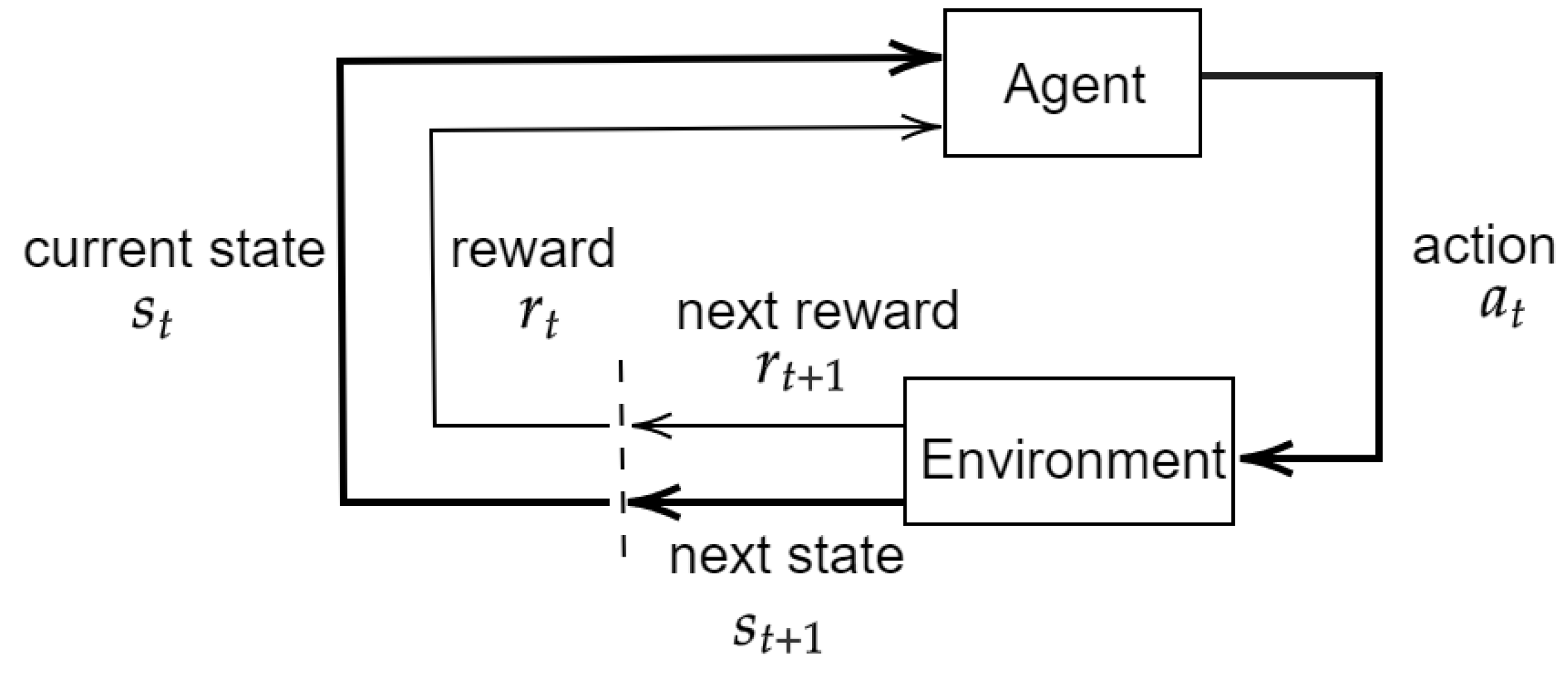
Chen et al. [40] used a deep Q-learning (DQN) model for an irrigation decision strategy based on short-term weather forecasts for rice. Daily observed meteorological data of the rice-growing period at three stations, including daily minimum and maximum temperature, average temperature, average wind speed, sunshine duration, average relative humidity, and precipitation were collected. The state-space consisted of $P_t$ is the predicted precipitation sequence for the next 7 days on day t, mm; $h_t$ is the water depth on day t, mm; $h_{m}in$ is the lower limit of water depth, mm; $h_{m}ax$ is the upper limit of water depth, mm; $H_p$ is the maximum allowable water depth after precipitation. In the action space, three possible actions were included, representing the fraction of the irrigation quota (irrigation to $h_{m}ax$) to be supplied to the field on day t. Action 0 returns 0%, action 1 returns 50%, and action 2 returns 100%. The reward is based on the rainfall use reward and the yield reward. The results of the DQN irrigation strategy compared to the results of the conventional irrigation strategy showed a significant reduction in irrigation water volume, irrigation timing, and drainage water without yield loss.

Alibabaei et al. [38] uses the DQN model to schedule irrigation of a tomato field in Portugal using climate Big Data. Historical data are collected from various sources and processed for use as input. Two LSTM models are trained on the obtained historical data to predict the total soil water in the soil profile for the next day and the tomato yield at the end of a season, respectively.

The trained LSTM models were used in the DRL training environment, which takes the current state (historical climate data) and action (amount of irrigation) and then returns the next state and reward. The reward was calculated as the net return and the Q-value was estimated using an LSTM model. The results show that the agent learns to avoid water waste at the beginning of the season and water stress at the end of the season. Compared to the threshold and fixed irrigation method, the DQN agent increases productivity by 11% and avoids water waste by 20–30%.

3.8.7. Automation in Agriculture

Deep learning is also being used to control sensors and robots that enable automation and optimization of agricultural processes. These robots can be used for a variety of purposes, including automated seeding, pesticide, and crop nutrient application, damage repair, irrigation, weed detection and removal, harvesting, etc.

Li et al. [52] used a deep-learning algorithm to quickly and accurately detect and locate longan fruit in imagery and pick the fruit with a UAV device. An RGB-D camera on the UAV was used to collect images of the fruits. As mentioned in the paper, one of the disadvantages of UAVs is that they are easily affected by local circulation and airflow when capturing images, resulting in blurred images of the fruits. In the preprocessing of the data, a Fuzzy image processing algorithm was used to remove the blurred images from the data set.

FPN, YOLOv3, YOLOv4, MobileNet-SSD, YOLOv4-tiny, and MobileNet-YOLOv4 models were trained on the images to detect and locate string fruits, simple fruits, and fruit branches. In the final phase, the detection results are mapped onto the optimized depth image to extract the contours and spatial information of the three targets. Based on this information, the drone can detect and locate the fruits and use them in harvesting. In general, the YOLO models had faster detection speed and achieved better accuracy than the FPN and SSD models. MobileNet-YOLOv4 achieved the best performance in terms of accuracy (mAP = 89.73) and inference time (68 s), while FPN achieved the worst performance.

To test the model in orchards, a picking platform was developed with a UAV, a Jetson TX2, an RGB-D camera, a set of scissors with clamps, and a support frame. The accuracy rate of successful harvesting in four cases was reported as 75, 75, 69.23, and 68.42.

Aghi et al. [106] presents a low-cost, energy-efficient local motion planner for autonomous navigation of robots in vineyards based on RGB-D images, low-range hardware (a low-cost device with low power and limited computational capabilities), and two control algorithms. The first algorithm uses the disparity map and its depth representation to generate proportional control for the robot platform. The second backup algorithm, based on a deep learning algorithm, takes control of the machine when the first block briefly fails and generates high-level motion primitives.

An Intel RealSense Depth Camera D435i RGB-D camera was used to capture images and compute the depth map on the platform. The video was captured in different terrain, quality, and time of day. Then, a light depth map-based algorithm processes the depth maps to detect the end of the vineyard row and then calculates control values for linear and angular velocities using a proportional controller. Since, as in many outdoor applications, sunlight negatively affects the quality of the results and interferes with the control provided by the local navigation algorithm, MobileNet was trained to classify whether the camera was pointed at the center of the end of the vineyard row or one of its sides, and it was used when the first algorithm failed due to outdoor conditions. The CNN model was trained with transfer learning and classified the images into three classes: Middle, Left, and Right. For the middle class, the video was taken in rows with the camera pointed at the center, and for the other two classes, the videos were rotated left and right with the camera at a 45-degree angle to the long axis of the row. The accuracy of the model on the test set was one. The model was trained on a small portion of the data set to investigate the significance of the size of the data set. The accuracy of the model decreased by 6% with the small data set.

Table 8. Feature descriptions of recent published papers in the field of “Water Management”.

References	Application	Data Used	Model	Metric Used	Model Performance
Saggi and Jain [103]	Estimation of evapotranspiration for irrigation scheduling.	Fourteen years of time-series data were used.	Multi-layer DL	RMSE	MLDL achieved better performance compared to RF, GLM, and GBM.
Zhang et al. [104]	Prediction of water table depth in agriculture areas	Daily meteorological data of 31 years for Hoshiarpur and 38 years for Patiala was considered for the study.	LSTM	$R^2$, RMSE	LSTM achieved better performance.
Loggenberg et al. [105]	Model water stress in vineyards	Stem water potential (SWP) was measured in the field using a pressure chamber. Images were acquired using the SIMERA HX MkII hyperspectral Sensor	RF and XGBoost	AC	RF outperformed XGBoost
Chen et al. [40]	Irrigation decision-making for rice base on weather forecasts	http://data.cma.gov.cn, accessed on 2 November 2021	DQN, CNN	The threat score (TS), missing alarm rate (MAR) and false alarm rate (FAR)	The DQN irrigation strategy compared to the results of the conventional irrigation strategy showed a significant reduction in irrigation water volume.
Alibabaei et al. [38]	Irrigation decision-making for tomato base on weather forecasts	www.drapc.gov.pt, accessed on 1 May 2021	DQN, LSTM	$R^2$-score, RMSE	Compared to the threshold and fixed irrigation method, the DQN agent increases productivity by 11% and avoids water waste by 20–30%.

Table 8. Feature descriptions of recent published papers in the field of “Water Management”.

References	Application	Data Used	Model	Metric Used	Model Performance
Saggi and Jain [103]	Estimation of evapotranspiration for irrigation scheduling.	Fourteen years of time-series data were used.	Multi-layer DL	RMSE	MLDL achieved better performance compared to RF, GLM, and GBM.
Zhang et al. [104]	Prediction of water table depth in agriculture areas	Daily meteorological data of 31 years for Hoshiarpur and 38 years for Patiala was considered for the study.	LSTM	$R^2$, RMSE	LSTM achieved better performance.
Loggenberg et al. [105]	Model water stress in vineyards	Stem water potential (SWP) was measured in the field using a pressure chamber. Images were acquired using the SIMERA HX MkII hyperspectral Sensor	RF and XGBoost	AC	RF outperformed XGBoost
Chen et al. [40]	Irrigation decision-making for rice base on weather forecasts	http://data.cma.gov.cn, accessed on 2 November 2021	DQN, CNN	The threat score (TS), missing alarm rate (MAR) and false alarm rate (FAR)	The DQN irrigation strategy compared to the results of the conventional irrigation strategy showed a significant reduction in irrigation water volume.
Alibabaei et al. [38]	Irrigation decision-making for tomato base on weather forecasts	www.drapc.gov.pt, accessed on 1 May 2021	DQN, LSTM	$R^2$-score, RMSE	Compared to the threshold and fixed irrigation method, the DQN agent increases productivity by 11% and avoids water waste by 20–30%.

Finally, the CNN model was optimized by discarding all redundant operations and reducing the floating-point accuracy from 32 to 16 bits. The accuracy of the optimized model was the same as the original and the time inference was improved. The proposed model was implemented on a robot and the tests were performed in a new vineyard scenario. The first algorithm can detect the end of the vineyard regardless of the direction of the long axis of the robot. When the first algorithm fails, the CNN model jumps in and detects the end of the vineyard.

Badeka et al. [107] trained YOLOv3 to detect grape crates in the field for use on robots harvesting grapes. The images of the crate were taken under natural field conditions. Three data enhancement techniques were used, including rotation, noise, processing, and blur processing. The model achieved an accuracy of 99.74% (mAP%) with an inference time of 0.26 s. To use the trained model on robots, it must be deployed on edge devices and report the inference time and accuracy of the model on these devices. Another interesting problem is that the robot can detect whether the box is full or not.

Majeed et al. [108] combined the DL model with mathematical models to detect cordons in grape canopies and determine their trajectories. Images were taken so that a tree trunk was approximately in the center of the field of view of a high-resolution camera (Sony Cyber-shot RX100 IV). A total of 191 images of random RGB images were captured from two different vineyard blocks with different cultivars. Each image in the dataset was classified into three classes: Background, Trunk, and Cordon (http://hdl.handle.net/2376/16939, accessed on 1 September 2021). Since the background pixels in the labeled images covered most of the images, a weight was assigned to each class in the preprocessing of the data, which was calculated using a median frequency class balancing method to avoid bias during training. Data augmentation and transfer learning techniques were used in this work.

A fully convolutional neural network (FCN) and SegNet with VGG and AlexNet backbones were trained to segment the cordons in the images. The FCN-VGG16 network achieved the best performance in terms of mean accuracy and $F_1$-score compared to the other networks. In the next step, the mathematical model including the Fourier model, Gaussian model, polynomial model, and sine sum model was applied to estimate the trajectory of the cordons. The sixth-order polynomial equation with an average $R^2$ value of 0.99 had the best fit for the trajectories of the cordons compared to the other mathematical models tested.

Pinto de Aguiar et al. [109] trained seven different DL models for detecting grapevine stems in two vineyards in Portugal. The trained models included Single Shot Multibox (SSD) MobileNet-V1 ($\alpha =0.75$), SSD MobileNet-V1 with different hyperparameters ($\alpha =0.75$), SSD MobileNet-V2, Pooling Pyramid Network (PPN) MobileNet-V1, SSDLite MobileNet-V2, SSD Inception-V2, Tiny YOLO-V3. In this work, Transfer Learning was applied using the COCO dataset. A dataset was created using a robotic platform. This dataset contains images captured in two different vineyards, using two cameras each, including the Raspberry Pi cameras and a conventional infrared filter, and the other camera Mako G-125C and an infrared filter (dataset is available at http://vcriis01.inesctec.pt/-DS_AG_39, accessed on 1 September 2021). After training the model, two edge devices, including Google’s USB Accelerator and NVIDIA’s Jetson Nano were used for real-time inference of the model in a real-world application. The advantage of NVIDIA’s Jetson Nano over Google’s USB Accelerator is that it supports floating points and more models. However, Google’s USB Accelerator outperformed NVIDIA’s Jetson Nano in terms of inference time (about 49 frames per second), average accuracy, and time to load models. The combination of edge devices and lightweight deep learning models makes the model DL applicable in practice.

Aguiar et al. [18] trained the SSD model using MobileNetv1 and MobileNetv2 as backbones to detect the stem in a vine. The model was deployed on an edge AI mode (Google’s USB Accelerator) in order to investigate accuracy and penetration. The images were acquired from four different vineyards in Portugal and published under the name VineSet. They contain RGB and thermal images of a single vineyard and include the annotations for each image (http://vcriis01.inesctec.pt/datasets/DataSet/VineSet.zip, accessed on 2 September 2021). A robotic platform AgRob V16 with a frontal stereo RGB camera and a frontal thermal camera was used to capture a video from which the images were extracted. Data augmentation methods such as rotation, translation, scaling, flipping, hue and saturation, Gaussian noise, and random combination were used to resize the dataset to a suitable size for the seepage learning method. Two training datasets were used to evaluate the effect of the training dataset size on the performance of the detectors. The original VineSet dataset and a small subset of it containing 336 non-augmented images were used. The SSD MobileNetv1 and the SSD MobileNetv2 trained with VineSet and using transfer learning achieved similar performance, a maximum AP of 84.16%, but the SSD Inception achieved an AP of 75.78. In terms of inference time, the MobileNets on the TPU achieved an average inference time of 21.18 ms and 23.14 ms, which was faster than SSD Inception. The performance of the models trained with a small dataset dropped significantly (with a maximum of AP = 34.42), reinforcing the importance of the dataset size for the performance of the deep learning model.

The SSD MobileNet-V1 trained with VineSet was published on the Google Colaboratory platform (https://colab.research.google.com, accessed on 1 September 2021) to help researchers automatically label the new dataset and then manually correct the labeling. Labeling the data is one of the challenges of using the DL model. In this way, labeling the images of the trunk becomes less time-consuming.

Table 9. Feature descriptions of recent published papers in the field of “Automation in agriculture”.

References	Application	Data Used	Model	Metric Used	Model Performance
Li et al. [52]	Pick longan fruits with a UAV device	A RGB-D camera on the UAV device used to capture images from the field.	FPN, YOLOv3, YOLOv4, MobileNet-SSD, YOLOv4- tiny and MobileNet-YOLOv4	mAP, AC, R, P	The accuracy rate of successful harvesting using a picking platform in four cases was reported as 75, 75, 69.23, and 68.42.
Aghi et al. [106]	Local motion planner for autonomous navigation of robots in vineyards	A camera D435i RGB-D camera was used to capture images from the field.	MobileNet	AC, R, P, $F_1$-score	The accuracy of the model on the test set was given as one and it was decreased 6% with the small dataset.
Badeka et al. [107]	Detect grape Crates in the field	The images of the crate were taken under natural field conditions	YOLOv3	AC	The model achieved an average detection rate of 99.74%.
Majeed et al. [108]	Detect cordons in grape canopies and then de- determine their trajectories	Images were taken so that a tree trunk was approximately in the center of the field of view of a high-resolution camera	FCN and Seg-Net with VGG and AlexNet	R, P, $F_1$-score	The FCN-VGG16 network achieved the best performance in terms of mean accuracy and F_1 score compared to the other networks.
Pinto de Aguiar et al. [109]	Detect grapevine trunk in two vineyards in Portugal using TPU and NVIDIA’s Jetson Nano	This dataset contains images captured in two different vineyards, using two cameras	FCN and Seg-Net with VGG and AlexNet, SSD MobileNet-V2, Pooling Pyramid Network, MobileNet-V1, SS- DLite MobileNet-V2, SSD Inception-V2, Tiny YOLO-V3.	IOU, $F_1$-score	SSD MobileNet-V2 on the TPU coral with an average precision of 52.98% and approximately 49 f/s achieved the best
Aguiar et al. [18]	Detect the trunk in a vine	The images were acquired from four different vineyards in Portugal	SSD MobileNetv1, SSD MobileNetv2, SSD Inception	mAP, IOU, R	The SSD MobileNetv1 and the SSD MobileNetv2 achieved similar performance (maximum AP of 84.16%), but the SSD Inception achieved an AP of 75.78.

Table 9. Feature descriptions of recent published papers in the field of “Automation in agriculture”.

References	Application	Data Used	Model	Metric Used	Model Performance
Li et al. [52]	Pick longan fruits with a UAV device	A RGB-D camera on the UAV device used to capture images from the field.	FPN, YOLOv3, YOLOv4, MobileNet-SSD, YOLOv4- tiny and MobileNet-YOLOv4	mAP, AC, R, P	The accuracy rate of successful harvesting using a picking platform in four cases was reported as 75, 75, 69.23, and 68.42.
Aghi et al. [106]	Local motion planner for autonomous navigation of robots in vineyards	A camera D435i RGB-D camera was used to capture images from the field.	MobileNet	AC, R, P, $F_1$-score	The accuracy of the model on the test set was given as one and it was decreased 6% with the small dataset.
Badeka et al. [107]	Detect grape Crates in the field	The images of the crate were taken under natural field conditions	YOLOv3	AC	The model achieved an average detection rate of 99.74%.
Majeed et al. [108]	Detect cordons in grape canopies and then de- determine their trajectories	Images were taken so that a tree trunk was approximately in the center of the field of view of a high-resolution camera	FCN and Seg-Net with VGG and AlexNet	R, P, $F_1$-score	The FCN-VGG16 network achieved the best performance in terms of mean accuracy and F_1 score compared to the other networks.
Pinto de Aguiar et al. [109]	Detect grapevine trunk in two vineyards in Portugal using TPU and NVIDIA’s Jetson Nano	This dataset contains images captured in two different vineyards, using two cameras	FCN and Seg-Net with VGG and AlexNet, SSD MobileNet-V2, Pooling Pyramid Network, MobileNet-V1, SS- DLite MobileNet-V2, SSD Inception-V2, Tiny YOLO-V3.	IOU, $F_1$-score	SSD MobileNet-V2 on the TPU coral with an average precision of 52.98% and approximately 49 f/s achieved the best
Aguiar et al. [18]	Detect the trunk in a vine	The images were acquired from four different vineyards in Portugal	SSD MobileNetv1, SSD MobileNetv2, SSD Inception	mAP, IOU, R	The SSD MobileNetv1 and the SSD MobileNetv2 achieved similar performance (maximum AP of 84.16%), but the SSD Inception achieved an AP of 75.78.

4. Discussion

Deep learning is already being used in various areas of agriculture, but it is still far from being widely applied in agriculture. In this paper, we reviewed 46 recent research papers to examine the challenges of using deep learning in agriculture. Figure 13 shows the pie chart of the researched papers based on the application domain.

The following challenges can be pointed out from the reviewed articles. The most critical point concerns the dataset. Training the model with a small dataset can lead to significant failures [18,72,106] and even with transfer learning and data augmentation, training the model may require a sufficient amount of data [55]. The presence of the image under field conditions in the data set is very important [63]. Therefore, collecting authentic field images and datasets under different conditions is the first and most important step. Using open-source datasets, sharing the dataset with other researchers, data augmentation, and transfer learning properly can help to overcome these challenges [71,77].

In addition, agricultural image datasets are more complex due to outdoor conditions, the object of interest usually occupying a very small and uncentered part of the image, similarity between objects and background, blocking the object with leaves and branches, multiple objects in one image, and many more [31,63,65,68,79,82]. To be applicable in the real world, the dataset should fully represent the state of the environment. In some cases, such as variable illuminance, data augmentation may also be helpful.

The type of input affects the performance of the model [55,62,88,92]. Removing background from images [55], using different color spaces and vegetarian indices as input [62], detecting crop at different growth stages [81], adding vegetarian indices to the input [30,86], cropping the input image [91], and data from different climate types [99] change the performance of the model. The size of the input also affects the runtime and accuracy of the model [62,79]. Therefore, it is challenging to determine the best input set for the specific task.

Labeling large amounts of data is expensive and time-consuming [55]. In addition, there are some tasks, such as those related to plant diseases, that can only be performed by specialists in the field. Even when using open-source datasets with already annotated data, there is no way to find out who actually did the annotation. As it was seen in several papers, data augmentation and transfer learning are ways to avoid labeling a large dataset, but labeling a small dataset is still time-consuming [55]. Unsupervised and semi-supervised learning methods can be of great help but need further investigation in this area [35,36,61,83].

When choosing a model for a task, there is a tradeoff between accuracy and inference time [26,34,65,67,77,96]. Depending on the application, the model can be chosen.

Neither environment is similar in the field of agriculture, and each environment and problem requires its own dataset, and therefore the DL model may not be universally applicable, i.e., if a model has been trained with a dataset from a particular site or a dataset from an open-source site such as ImageNet, it may not be able to be used at another site, or accuracy may decrease when applied to the dataset collected in the real world [12,69]. The changes in the visual appearance of the images in the training and test dataset could lead to a decrease in model performance [30]. One way to overcome this is to retrain the already trained model with a small dataset from the new environment [86].

The design of deep models is complex and they are referred to as black boxes [7]. One of the challenges in training DL models is that a system with very high computational power (GPU) is needed [7]. Moreover, the performance of these models depends on the choice of hyperparameters, loss functions, and optimization algorithm [60,67]. Algorithms such as Bayesian optimization [110] can help to find the right hyperparameters [102]. Google researchers used neural architecture search (NAS) algorithm [111] to find state of the art MobilenetV3 [112]. NAS is a method that searches among all possible combinations of submodules that can be repeatedly assembled to obtain the entire model with the best possible accuracy.

The other challenge relates to the real-time applicability of the models. Most deep learning models have many parameters that need to be trained, and after training the model, inference of the model is not made in real-time. In some applications, such as using a robot for harvesting, time inference is essential. As we see in this work, most of the models are implemented and tested on the PC, which requires power and it is impractical in real applications. Moreover, implementation on devices such as smartphones still, brings various challenges that need to be considered, such as memory consumption, speed, etc. Single-stage detection models such as YOLO and SSD, lightweight classification models such as MobileNet, the development of edge devices such as Raspberry Pi and Jetson nano, and the use of cloud computing have made it possible to deploy Deep Learning models in real-world applications and practical ways [34,52,72,86,109]. The quantization method can be also used to compress the model size and improve the detection speed [82].

On small farms, the use of some methods is sometimes impractical because farmers must have some knowledge to interpret the results obtained. For example, the model that predicts soil moisture for irrigation scheduling requires a human expert to use this information to determine the best time and amount of water for irrigation. As mentioned earlier, Deep Reinforcement Learning is showing great success in several areas as a promising model for building smart farms in several areas [39]. The model can be trained to make decisions about when and how much to irrigate [38,40]. Information generated by IoT devices also helps farmers track agricultural operations and make better decisions to improve agricultural productivity [97].

5. Conclusions

This paper discussed some recent work on the application of DL to agriculture and biodiversity and highlighted some challenges in this area. More sustainable agriculture and the promotion of biodiversity in agricultural systems can be achieved by reducing the use of agrochemicals, low pesticide use and organic farming, appropriate crop rotations, small-scale fields, and the preservation of natural spaces between agroecosystems [113]. As mentioned, this can be achieved through the new IoT technology in combination with the new biodiversity algorithms and Artificial Intelligence model. They can be used to detect and control species and also to improve ecosystem state and thus productivity having to resort to the use of environmentally damaging practices.

The novelty of the application of DL models and the challenges identified in agriculture demonstrates the need for further research. CNN is the most widely used DL model in agriculture. The use of new methods, such as attention mechanisms, new lightweight models, single-stage detection models, can improve the performance of the model, as a slight improvement in accuracy and run time can significantly improve the final results.

In the future, we expect to develop or improve models that help farmers make crop management decisions. These models can be integrated into decision support tools, and these tools can guide users through precise steps and suggest optimal decision paths. It is expected that the development of these models will also enable biodiversity monitoring. Consequently, the adoption of new sustainable practices supported by DL models and biodiversity monitoring will help manage the farm with minimal human intervention and greater effectiveness.