Article

Lunar Crater Detection on Digital Elevation Model: A Complete Workflow Using Deep Learning and Its Application

Faculty of Information Technology, Macau University of Science and Technology, Taipa, Macau 999078, China
*
Author to whom correspondence should be addressed.
These authors contributed equally to this work.
Remote Sens. 2022, 14(3), 621; https://doi.org/10.3390/rs14030621
Submission received: 16 December 2021 / Revised: 21 January 2022 / Accepted: 24 January 2022 / Published: 27 January 2022

Abstract

:
Impact cratering process is the major geologic activity on the surface of the Moon, and the spatial distribution and size-frequency distribution of lunar craters are indicative to the bombardment history of the Solar System. The substantial efforts on the development of automated crater detection algorithms (CDAs) have been carried out on the images from the remote sensing observations. Recently, CDAs via convolutional neural network (CNN) on digital elevation model (DEM) has been developed as it can combine the discrimination ability of CNN with the robust characteristic of the DEM data. However, most of the existing algorithms adopt a traditional two-stage detection pipeline including an edge segmentation and a template matching step. In this paper, we attempt to reduce the gap between the existing DEM-based CDAs and the advanced CNN methods for object detection, and propose a complete workflow including an end-to-end deep learning pipeline for lunar crater detection, in particular for craters smaller than 50 km in diameter. Based on the workflow, we benchmark nine representative CNN models involving three popular types of detection architectures. Moreover, we elaborate on the practical application of the proposed workflow, and provide an example method to demonstrate the performance advantage in terms of the precision ( 82.97 % ) and recall ( 79.39 % ). Furthermore, we develop a crater verification tool to manually validate the detection results, and the visualization results show that our detected craters are reasonable and can be used as a supplement to the existing hand-labeled datasets.

1. Introduction

In the past few decades, several missions have been carried out to explore the Moon, including the detection of crater structure on the lunar surface. Due to no tectonic activities occurring on the Moon, the structures of most impact craters are well preserved, even including the ones formed four billion years ago [1,2]. As a typical geomorphologic structure over the lunar surface, the impact craters record the bombardment history of the inner Solar System. As the bombardment flux of the Solar System decreases with the increases of time, the density and size-frequency distribution of craters over the lunar surface directly provide the critical information on the relative age of the mare units on the Moon because older mare unit has massive impact records, whereas the younger one has less impact imprint [3,4]. Therefore, the spatial crater distribution and crater size-frequency distribution is critical to understand the bombardment history of the Moon, from which the impact flux of the Solar System can be well derived. As there are hundred-million impact craters on the Moon with the diameter range from centimeter to thousand kilometers, how to count their size and spatial distribution is a difficult problem. The conventional method that is still used in the planetary researches currently is the manual detection method, which heavily relies on human experts to annotate lunar craters by using visual inspection of images and DEMs. The manual detection is very time-consuming and is difficult for exhaustive coverage, in particular for small or overlapping craters at specific geographic region [2,5].
In order to develop an efficient detection method with a high accuracy, the automated crater detection algorithm (CDA) has been widely considered by numerous researchers. According to the target data, the developed CDAs can be divided into two categories: (1) remote sensing image-based CDA and (2) digital elevation model (DEM)-based CDA. Generally, the optical images from the remote sensing observations of lunar surface with a high resolution could be more easily acquired than the DEM map with the similar resolution because the latter highly relies on the interpolation of the observations. Therefore, most of previous works prefer to employ the optical image as the dataset to study the crater detection method [6,7,8,9,10]. However, the remote sensing observed images are normally disturbed by unconstrained factors, such as illumination of the Sun, which increases the difficulty of the crater detection because the complicated terrains on the lunar surface have significant effects on the optical images and the detection error therefore increases [11]. In contrast, the DEM map is a composite of physical elevation data that describes the terrain variations and provides the actual position and height information. More importantly, the DEM map can avoid the uncertain optical error with robust data quality as it is not influenced by the illumination. As a consequence, the DEM-based CDA, such as the morphology-based approaches [12,13,14,15], the traditional machine learning methods [16,17], and the convolutional neural network (CNN) models [18,19,20,21], has become popular recently.
With the quick development of deep learning in the field of computer vision, the CNN models have demonstrated impressive performances on many vision tasks such as image classification [22], semantic segmentation [23], and object detection [24]. The major reason for their successful applications in the aforementioned fields is that CNN replaces the raw pixel data or the hand-crafted feature descriptors such as Scale-Invariant Feature Transform (SIFT) [25] and Histogram of Oriented Gradients (HOG) [26], with the feature representations learned from the expert-annotated dataset. Due to the data-driven nature, the CNN models can quickly adapt to different complex scenarios through a training process with the given labels, and generalize well to new data with the same distribution as the annotated data.
In the planetary science, the CNN model has been developed for automatic crater detection for the remote sensing observed images. In the early works [18,19,27], CNN is applied as a binary classifier to perform crater/non-crater classification on the remote sensing images, such as High Resolution Imaging Science Experiment (HiRISE) for Mars, Lunar Reconnaissance Orbital Camera (LROC) and High Resolution Stereo Camera (HRSC) for the Moon, respectively. These works claim a high identification accuracy with CNN in comparison with other machine learning methods, such as the support vector machine (SVM). In addition, Wang et al. [28] developed a novel fully convolutional neural network (FCN) for crater classification and position regression at the cell level by utilizing the HRSC images. Hashimoto and Mori [29] adopted U-Net [30] and the generative adversarial network to perform the grid-based crater classification on the LROC images. Recently, some works began to combine the identification ability of CNN with the robust characteristic of DEM. Silburt et al. [20] proposed a classic DEM-based CDA using deep learning, which includes a U-Net model for edge segmentation and a template matching algorithm for crater extraction. Ali-Dib et al. [21] used a general instance segmentation framework [31] to detect craters while simultaneously producing their masks. Jia et al. [32] combined an improved R-FCN and the transfer learning method for crater detection by using multiple data sources. More recently, some works [33,34,35] aimed to improve the method [20] by designing a new CNN with the similar structure as Unet.
However, we found that most of recent methods involve a two-stage pipeline processing as shown in Figure 1, in which an image patch is first input to a CNN model for edge segmentation through a forward calculation, and then the crater regions are extracted by performing a template matching algorithm on predicted masks. The template matching algorithm is computationally expensive as it has to calculate the matched probability of each segmentation target by iteratively sliding a group of ring templates with a discrete size distribution on an image patch. By contrast, there have been many works [24,36,37,38] proposed for object detection by directly predicting the position and size of a visual target.
In this work, we attempt to reduce the gap between the existing DEM-based CDAs and the advanced methods for object detection, and propose a complete workflow with an end-to-end deep learning pipeline to focus on the detection of craters smaller than 50 km in diameter on the DEM data. The workflow consists of four steps as follows:
  • In data preparation, a global DEM image is divided into a less number of sub-region images than the previous work [20] through a carefully designed grid cropped strategy. The new strategy can not only improve the detection rate of lunar craters by exploiting their size compensation, but also effectively reduce the cost of computation in both inference and post-processing steps as the number of each duplicate crater is reduced in an order of magnitude.
  • In the detection process, the cropped DEM images are input into a CNN model for joint detection of multiple lunar craters, which predicts their classification probabilities and location coordinates in an end-to-end manner.
  • During the post processing step, we merge all the detected craters while transforming their pixel coordinates to the geographical coordinates, and remove the duplicate craters by using a non-maximum suppression (NMS) algorithm before and after the merger.
  • In performance evaluation, we adopt the Average Precision (AP), a standard detection metric for the object detection task. Comparing to the single precision and recall metrics usually used in previous works [20,21], the AP metric can fully verify the detection performance of a CDA by considering a full range of precision and recall rates.
Based on the workflow, we use three popular types of object detection architectures with nine advanced CNN models [24,36,37,38,39,40,41,42,43] in the detection process, and build a new benchmark for lunar crater detection on the DEM data by comprehensively comparing the performances of all these CNN models. In order to verify the effectiveness of our workflow in practical application, we provide an example method and show that the automatically detected craters have a better overall performance with respect to precision ( 82.97 % ) and recall ( 79.39 % ) on the hand-labeled datasets than the recent DEM-based method [20]. In addition, we develop a crater verification tool to manually validate the detection results and find some newly identified lunar craters missed in the hand-labeled datasets. The visualization results show that the size-frequency distribution of the detected craters (D < 50 km) is almost similar to the labeled craters on the lunar surface; therefore, our detected craters can be used as a supplement of the hand-labeled datasets for the lunar community to investigate the bombardment history of the Moon, even the inner Solar System.
The rest of the paper is organized as follows: We introduce the proposed workflow in Section 2. The experimental protocol and results are given in Section 3. The practical application of the workflow is discussed in Section 4. Our conclusions is presented in Section 5.

2. Methods

In this section, we will describe our proposed workflow with details, which includes the steps of data preparation, crater detection process, post processing, and model evaluation.

2.1. Data Preparation

In this work, we used the DEM data from the Lunar Orbiter Laser Altimeter (LOLA) onboard Lunar Reconnaisance Orbiter (LRO) and the Terrain Camera (TC) on Kaguya (SELENE), which is released by the LOLA and Kaguya teams [44]. The DEM data is a near-global elevation map with a resolution of 512 pixels/degree that represents the lunar terrain elevation with a latitude range between 60 and 60 and a full range of longitude. For the crater information (position and size), we used the two released hand-labeled datasets, in which Povilaitis et al. [5] annotated the craters with a diameter between 5 and 20 km based on the LRO Wide Angle Camera (WAC) DEM data [45] with a resolution of 303 pixels/degree, and Head et al. [2] exploited the craters for a diameter larger than 20 km according to the LOLA DEM data with a resolution of 64 pixels/degree. We follow the work of Silburt et al. [20] to transform the resolution and bit depth of the original global image from 184,320 × 61,440 pixels with 16 bits/pixel to 92,160 × 30,720 pixels with 8 bits/pixel. The image is equally divided into three local images in the longitude ranges from 180 to 60 , from 60 to 60 and from 60 to 180 for the training, validation and test in the following steps, respectively.
To get a satisfied input for the follow-up CNN models, the local DEM images have to be cropped into multiple sub-region patches with a small size. A reasonable cropped strategy is required because the following problems have to be considered: (1) The integrity of craters around the edge of image patches is easily destroyed. (2) It is hard to select a suitable size of cropped window for image cropping. Generally, a large cropped patch contains more craters with an unbalanced size distribution that increases the learning difficulty of models, while a small one has less craters in a narrow size range but likely loses the partial terrain information for large craters.
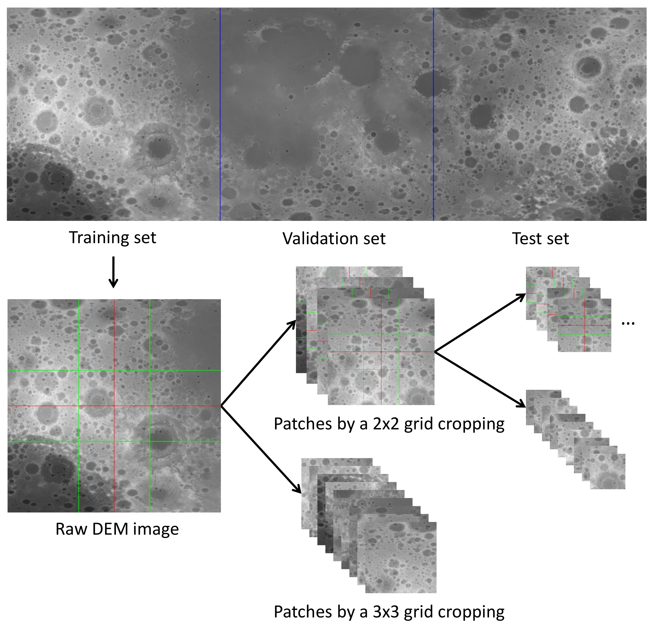
Inspired by the works [24,46] that use multiple scales of an image pyramid to improve the detection performance, we propose a multi-scale grid cropping strategy that could reduce the scale sensibility of a CNN model by providing multiple scales of each crater from different image patches in both the training and detection procedures. As shown in Figure 2, each local image with 30,720 × 30,720 pixels is divided into 2 2 n sub-region images with the same resolution, where n { 1 , 2 , 3 , 4 , 5 , 6 } and represents 6 different sizes of cropped windows, i.e., 15,360 × 15,360, 7680 × 7680, 3840 × 3840, 1920 × 1920, 960 × 960 and 480 × 480 pixels. In order to compensate for partial structure of craters near the edges of cropped images, we further divide each local image or each sub-region image (except for that with the smallest size) into 9 identically sized patches by using 6 additional cropped windows, i.e., 10,240 × 10,240, 5120 × 5120, 2560 × 2560, 1280 × 1280, 640 × 640 and 320 × 320 pixels. For an example, Figure 2 shows the cropped results of a local image for training, where the red and green dotted lines denote two stages of image cropping through the 2 × 2 and 3 × 3 grids, respectively. These cropped images are resized to a resolution of 512 × 512 pixels. After the cropping process, we can get 17,745 sub-region images on the training, validation, and test sets. All the craters in each image are annotated with the radii lengths and the center coordinates that are derived from their spatial locations and diameters in the hand-labeled datasets. As the original DEM image is released in a Mercator projection, which leads to a noticeable image distortion and unreal pixel coordinates for the cropped images, we reformat these images and the crater annotations by applying an orthographic projection, which are implemented by the Cartopy Python package [47]. In addition, we use a linear transformation to improve the contrast of these images and enhance the visual differentiation of the craters.

2.2. Crater Detection Process via Convolutional Neural Network

In the detection process, we formulate the lunar crater detection task as the problems of target classification and associated location regression, which have been widely explored by the previous object detection methods [24,36,37,38,39,40,41,42,43]. According to the architecture design of the detection network, these previous methods can be classified into three categories: Region-based Detection Network (RDN), Anchor-based Detection Network (ADN), and Point-based Detection Network (PDN).

2.2.1. Region-Based Detection Network (RDN)

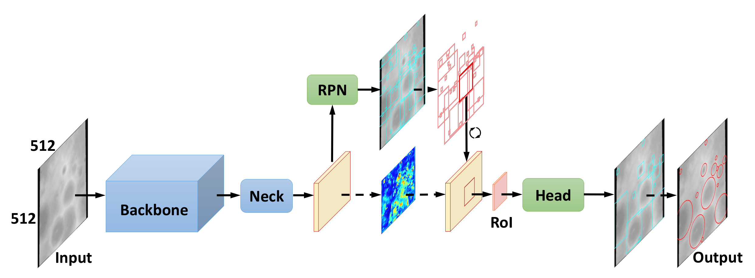
As shown in Figure 3, the RDN architecture contains four key modules: Backbone, Neck, Region Proposal Network (RPN), and Head. Given an input image patch, the backbone module is used to generate the basic feature maps through a forward calculation. In general, the backbone module is a classic CNN model that is pre-trained on the Imagenet [48] dataset for image classification. Several previous works [49,50] indicated that such feature maps can capture hierarchical semantic information and are suitable for different visual tasks. The neck module is an optional structure that further exploits the feature hierarchy of CNN to extract multi-scale feature maps with different receptive fields, and provides scale-specific context information for different objects. The RPN module can be considered as a sliding-window object detector, which is implemented by performing a 3 × 3 convolution and two sibling 1 × 1 convolutions on each single-scale feature map to generate the classification and regression maps. Each pixel in the classification map is a probability for crater/non-crater classification, while each pixel in the regression map denotes the coordinate offsets of a pre-defined anchor box described in Section 2.2.2. Through the RPN module, we can get a set of candidate crater targets called region proposals, and then apply the region-of-interest (RoI) extractor to get region-wise features corresponding to the positions of these region proposals on basic feature maps. The head module is designed as a sub-network followed by two parallel fully-connected layers. It can iteratively receive the proposal features and output a refined classification probability as well as associated coordinate offsets of each region proposal.
In this work, we adopt three popular RDN models: Faster R-CNN [24], Faster R-CNN + FPN [37], and Cascade R-CNN [39] for lunar crater detection. Faster R-CNN uses partial convolutional layers of the ResNet-50 model from the work [51] as the backbone module, and adopts the final convolutional layer with a global average pooling as the body of the head module. Based on the output feature maps with the strides of 16 pixels, the RPN module defines 15 types of anchor boxes having areas of { 32 2 , 64 2 , 128 2 , 256 2 , 512 2 } pixels and aspect ratios {1:2, 1:1, 2:1}. Faster R-CNN + FPN extends the work [24] by exploiting all convolutional layers of the ResNet-50 model as the backbone module, a feature pyramid network (FPN) as the neck module, and two fully-connected layers as a sub-network in the head module. The FPN neck module applies the top-down and skip connections to the backbone module, and generates five scales of feature maps that have strides of {4, 8, 16, 32, 64} pixels with respect to the input image. It is worth mentioning that FPN has been developed as an important component in recent detection models because it can provide multi-scale feature maps with strong semantics for detecting different sizes of targets. The RPN module would evenly assign the anchor boxes with the same setting as Faster R-CNN to each single-scale feature map from FPN. Cascade R-CNN follows the major design of Faster R-CNN + FPN and uses three cascaded head modules with the same structure, each of which aims to refine different qualities of region proposals by using a set of gradually increased thresholds {0.5, 0.6, 0.7} to filter the ones with the mismatched Intersection-over-Union (IoU) overlap with the ground-truth (GT) target. During the training of all the RDN models, the RPN and head modules use the sigmoid cross-entropy loss and the softmax loss for crater classification respectively, and adopt the smooth L1 loss [46] for coordinate offset regression of identified craters.

2.2.2. Anchor-Based Detection Network (ADN)

Although the RDN architecture has demonstrated excellent detection performance on various complex datasets such as PASCAL VOC [52] and MS COCO [53], the refinement process of region proposals has high computation cost, especially if an input image includes a large number of objects. To implement an one-stage detection process, a simplified RDN have been developed as a new detection architecture called ADN by removing the region-based refinement sub-network. At the ADN architecture, the head module follows the design of the RPN module to receive different scales of feature maps from the neck module, and generate the crater classification and location regression maps associated to each prior anchor box. As shown in Figure 4, the red rectangles denote the anchor boxes with different sizes and aspect ratios, which are evenly tiled on each location of output maps to match the GT boxes described by the green rectangles. We can detect lunar craters with a wide size distribution by aggregating the classification probabilities and coordinate offsets of all the anchor boxes. Comparing to the RPN module in RDN, ADN tends to apply more reasonable anchor assignment and learning strategies to improve the detection performance.
To evaluate the performance of the ADN architecture for lunar crater detection, we select three typical ADN models which are called SSD [36], RetinaNet [41], and YOLOv3 [40] respectively. SSD uses the VGG16 model from the work [54] as the backbone module, and introduces an SSD-style pyramid as the neck module by adding ten new convolutional layers. The SSD-style pyramid provides seven scales of feature maps with a wider range of stride lengths than those in the FPN module. Each scale of feature map is fed to an individual head module that contains two parallel 3 × 3 convolutions. According to the anchor assignment strategy in SSD, the corresponding output map is tiled by six or ten types of anchor boxes covering the size range 20–500 pixels. During the training, SSD adopts the softmax loss and the smooth L1 loss to learn the classification and regression tasks, respectively. RetinaNet follows the designs of the backbone and neck modules from Faster R-CNN + FPN, and builds a deeper head module that consists of two separate sub-networks with five 3 × 3 convolutions. For denser anchor covering than RPN, RetinaNet assigns nine types of anchor boxes with the size range 32–813 pixels and the original aspect ratios {1:2, 1:1, 2:1} in each scale of output map. In the training process, RetinaNet replaces the softmax loss with the focal loss [41] to improve the classification of hard samples. YOLOv3 adopts Dartnet-53, a more efficient CNN model than ResNet-50 as the backbone module, and uses a normal neck module with three scales of output feature maps by applying similar operations as FPN. The head module consists of seven alternative 1 × 1 or 3 × 3 convolutions, and uses the sigmoid cross-entropy loss and the sum of squared error loss to learn the classification and regression tasks, respectively. Instead of the hand-designed anchor boxes, YOLOv3 uses nine dimension clusters as anchor boxes by running the k-means clustering of GT bounding boxes on the training set.

2.2.3. Point-Based Detection Network (PDN)

The PDN architecture is another popular detection architecture, and focuses on conducting target classification and point offset regression in a per-pixel prediction fashion. Comparing to RDN and ADN, PDN does not rely on the setting of prior anchor boxes, which usually results in additional hyper-parameters with respect to anchor shapes and anchor assignment strategies. These hyper-parameters are not always applicable for all the datasets because they are carefully tuned to make anchor boxes densely cover the targets with a regular distribution. As seen in Figure 5, the PDN architecture has similar network structures of the backbone and neck modules as the RDN and ADN architectures. Given a single-scale feature map, the head module of PDN only outputs a single branch of detection results including a classification map and a group of regression maps, rather than multiple branches of ones associated to different types of anchor boxes.
Recently, the PDN architecture has been proved to be effective in different detection tasks such as the face detection and the pedestrian detection [55]. In our experiments, we use three advanced PDN models: FoveaBox [42], FCOS [38] and RepPoints [43] as parts of the benchmark methods for lunar crater detection. Following the structure of RetinaNet, these models adopt the ResNet-50 model as the backbone module, and build a FPN neck module to extract five scales of feature maps with strides of {8, 16, 32, 64, 128} pixels, each of which is responsible for the prediction of the targets with a specific size range. In FoveaBox and FCOS, the head module performs similar convolution operations as that of RetinaNet, and produces a classification probability and four point offsets at each location in output maps. These offsets denote the distances between the current location and four edges of an associated target box. The main difference is that FCOS uses an additional convolution layer in parallel with the classification layer to predict the deviation of each location to the center of the target box. During inference, the deviation is used to down-weight the probability of a predicted box far away from the center of the corresponding target. RepPoints builds a two-stage head module composed of a classification sub-network and two location sub-networks. At the first stage, the first location sub-network conducts four 3 × 3 convolutions and a 1 × 1 convolution to compute nine point offsets for the prediction of a coarse bounding box at each output location. At the second stage, the classification sub-network and the second location sub-network exploit these point offsets to extract feature maps by performing three 3 × 3 convolutions and a 3 × 3 deformable convolution, and then apply a 1 × 1 convolution to generate a classification probability and nine refined point offsets at the corresponding location, respectively. In the training process, all the PDN models adopt the focal loss and the smooth L1 loss to learn the classification and regression tasks respectively, except that FCOS uses the IoU loss as in the work [56] to learn point offset regression, and employs the sigmoid cross-entropy loss to learn center deviation regression.

2.3. Post Processing

When any detection network mentioned above is used, there are quite a number of output bounding boxes having different IoU overlaps with each other. Therefore, an additional filter is required to get a set of unique targets from the detection results of each cropped image. Here, we follow the work [57] and adopt a greedy NMS algorithm which is detailed as follows. Firstly, all candidate boxes are sorted by their classification probabilities in reverse order. Based on this step, we take the first one as a detected target and calculate all the IoU values with other bounding boxes. If the IoU valve is greater than a predefined threshold, the corresponding box would be removed as a repeated target. Once again, we take the second one with highest classification probability from the remaining candidate boxes, and eliminate all associated repeated targets. This process is executed repeatedly until each bounding box is labeled as the detected target.
For practical purposes, we would transform the coordinates of the detected bounding boxes from the rectangle form ( x 1 , y 1 , x 2 , y 2 ) to the circle form ( x , y , r ) by the following formulas:
x = x 1 + x 2 2 , y = y 1 + y 2 2 , r = ( x 1 x 2 ) + ( y 1 y 2 ) 4 ,
where ( x 1 , y 1 ) and ( x 2 , y 2 ) are the coordinates of two rectangle vertices at the top left corner and bottom right corner, respectively. ( x , y ) denotes the coordinate of the circle center, and r is the length of the corresponding radius.
To get the geographical coordinates ( L o n g , L a t , R ) of the detected craters from their pixel coordinates ( x , y , r ), we follow the work [20] and adopt the following conversion formulas:
L a t = Δ L a t Δ y ( y y 0 ) + L a t 0 , L o n g = Δ L a t cos ( π L a t 180 ) Δ y ( x x 0 ) + L o n g 0 , R = r Δ L a t C K D Δ y ,
where ( L o n g , L a t ) denotes the longitude and latitude of the crater center, and R is the kilometer length of the crater radius. The variables with subscript 0 represent the associated center coordinates of the cropped image. Δ L a t and Δ y are the ranges of latitude and pixel respectively along the vertical axis of the image center. C K D depicts a conversion relationship between degrees and kilometers on the Moon by the following formula:
C K D = 180 π R Moon ,
where R Moon is the kilometer length of the Moon’s radius.
When we obtain the geographical coordinates of all the craters scattered in different cropped images, we need to merge these sub-region results into a global crater collection. As we adopt a multi-scale grid cropping strategy for image cropping, the same craters will be detected in multiple image patches with different scales. Therefore, we introduce another required filtering process to remove the duplicate craters. This step is similar to the previous duplicate filter by using the NMS-based algorithm. However, we note that there are two main differences in comparison with previous step: (1) The craters are reformulated as circles represented by geographical coordinates with degrees (of longitude and latitude) and kilometers (of radius), while the previous filter tackles the carters as bounding boxes with pixel coordinates. (2) The new filter needs to consider all detected craters in a global DEM image rather than handling the duplicate craters in each sub-region image.
In the new duplicate filter, we would combine shape transformation with unit conversion in the IoU calculation, and a new formula to get the IoU value is derived as follows:
I o U = o v e r l a p π r 1 2 + π r 2 2 o v e r l a p ,
where o v e r l a p represents the intersection area of two craters, and is calculated according to their relative geographical positions:
o v e r l a p = 0 i f r 1 + r 2 d min π r 1 2 , π r 2 2 i f r 1 r 2 d r 1 2 α + r 2 2 β r 1 d s i n α o t h e r w i s e ,
where the first case represents two craters lie outside each other or touch externally, the second case indicates two craters lie touch internally or one lies completely inside the other, and the third case implies that they intersect at two points.
In this formula, α and β are the central angles of two craters corresponding to the intersection area:
α = a r c c o s r 1 2 + d 2 r 2 2 2 r 1 d , β = a r c c o s r 2 2 + d 2 r 1 2 2 r 2 d .
Here, r 1 and r 2 denote the radiuses of two craters, and d is the distance between their centers. The following equations are used to unify the radius and the distance in latitude (degree).
d = L o n g 1 L o n g 2 2 cos 2 π 180 L a t + L a t 1 L a t 2 2 ,
r = C K D r k m ,
where ( L o n g 1 , L a t 1 ) and ( L o n g 2 , L a t 2 ) are the longitude and latitude coordinates of two craters. To make the conversion error as small as possible in the distance calculation, we use the mid-point latitude L a t between the centers of the craters for the longitude conversion. r k m denotes the radius of a crater in kilometer, and is transformed to the radius r in latitude by Formula (3).

2.4. Model Evaluation

After the step of post-processing, we get all detected craters with geographical coordinates and classification probabilities in a global DEM image. In previous works [20,21], the precision, recall and F1 score metrics are used to evaluate the overall performance of CDAs, while the fractional error rates in latitude, longitude and radius are used to measure the accuracy of identified craters. We find that these metrics would inevitably rely on a specific confidence threshold for the crater decision. It is difficult to search an optimal hyper-parameter for different models and ensure a fair comparison among them. In this work, we follow the standard evaluation procedure from the PASCAL VOC and MS COCO challenges, and use the AP metric to validate the detected craters with geographical coordinates. Comparing to the previous metrics, AP denotes the area under the precision-recall (P-R) curve without the setting of the confidence threshold, and can be made a comprehensive assessment for the detection performance of models since it considers a full range of precision and recall rates. Moreover, we also use the AP metric to analyze the quality of detected craters by applying different IoU thesholds during the evaluation, which are responsible for quantifying the matching degree of a predicted crater and the corresponding GT target. The AP metric is implemented by the following steps:
  • Calculate a cumulative set of precision and recall values. We first sort all detected craters in reverse order with respect to their classification probabilities, and use Formula (4) with a pre-defined IoU threshold to calculate the cumulative numbers of true positives (TP) and false positives (FP) according to their maximum IoU overlaps with the associated GT targets. Note that we only regard the detected crater with the highest classification probability as TP when a GT target matches multiple predicted craters. And then, we can get the corresponding precision and recall values by using the following formulas:
    P r e c i s i o n = N T P N T P + N F P , R e c a l l = N T P N G T .
  • Draw the P-R curve with interpolation of all points. We first get the P-R scatter plot according to a given set of precision and recall values, and then interpolate the precision of each point by using the maximum precision whose recall value is greater or equal than the one of the current point. The interpolation formula is as follows:
    P ^ ( R n ) = max R ˜ : R ˜ R n P ( R ˜ ) ,
    where P ^ ( R n ) denotes the interpolated precision at recall R n .
  • Calculate the AP value. We can use the following formula to get the area under curve (AUC) of the P-R curve, which is the AP value for crater detection.
    A P = n R n R n 1 P ^ ( R n ) .

3. Results

In this section, we conduct extensive experiments for lunar crater detection and provide a detailed benchmark by evaluating and analyzing different CNN models.

3.1. Hyper-Parameter Setting

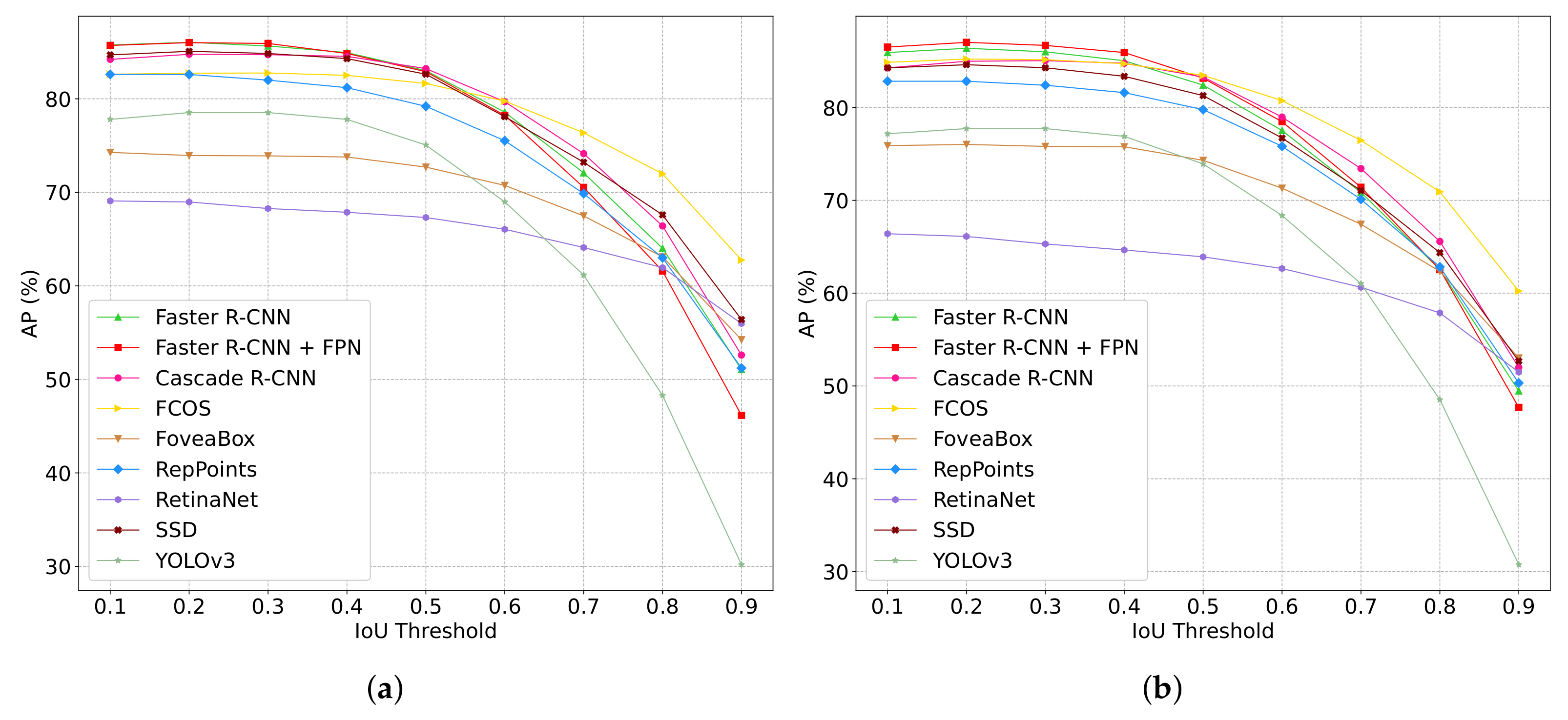
In the post processing of the workflow, there are two hyper-parameters called IoU threshold, which are involved in the NME algorithm to filter the duplicate craters before and after the merger of sub-region results, respectively. For the first hyper-parameter, we follow the standard setting in previous works and adopt a IoU threshold of 0.5 to remove the duplicate craters with pixel coordinates in each image patch. The value of the second hyper-parameter is associated with the real distribution of lunar craters with different degrees of overlaps, since it is used to remove the duplicate craters with geographical coordinates in a global DEM image. In this work, we perform a discrete exhaustive search of the second IoU thresholds in a possible range from 0.1 to 0.9 by evaluating all the models on the validation and test sets. Our results, as shown in Figure 6, indicate that the IoU threshold of 0.2 is more reasonable because all the models can almost achieve the optimal detection performance on both sets.

3.2. Experimental Results

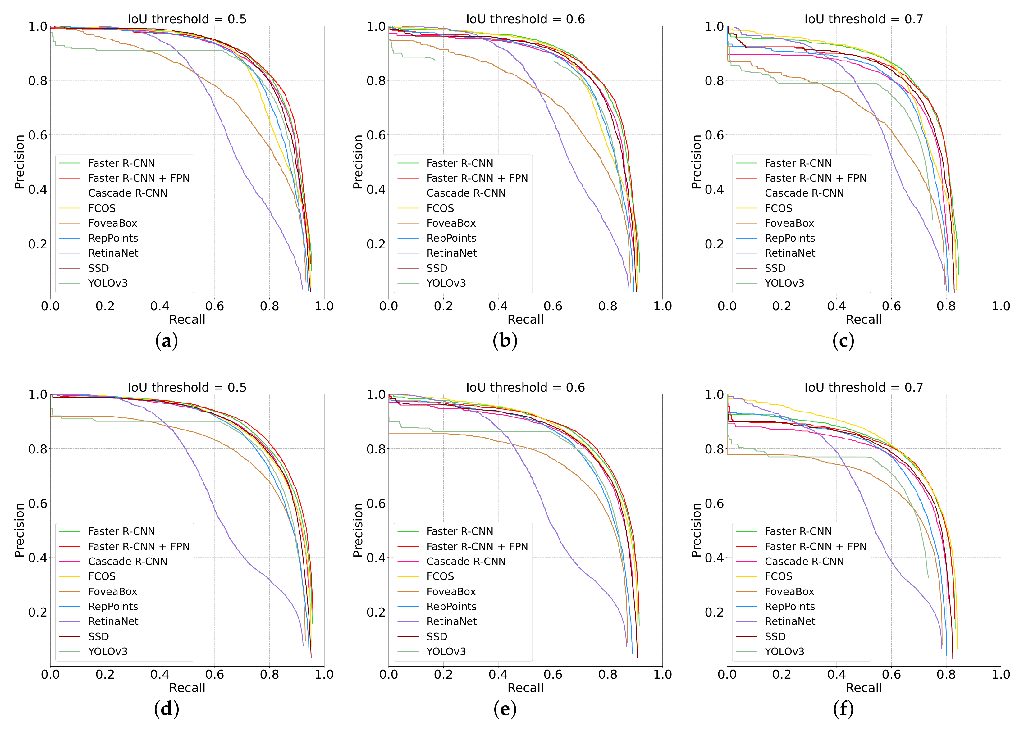
To evaluate the overall performance of selected representative models, we conduct three groups of experiments on the validation and test sets to calculate the AP metric of each model by using different matching thresholds also called IoU threshold. As shown in Table 1, we found that Faster R-CNN and Faster R-CNN + FPN can get the excellent performance on both sets under the standard setting of IoU threshold (IoU thr = 0.5), and consistently maintain the advantage comparing to most of models, even if IoU threshold is gradually increased (IoU thr = 0.6 and IoU thr = 0.7). It means that both the models have a better trade-off between each pair of precision and recall, and can detect the craters with more accurate position and radius than other models. In addition, we also observe that SSD and FCOS have better performance than other methods based on the ADN and PDN architectures. Especially, the FCOS model shows a competitive regression ability since it gets the highest AP value on the test set when we use a IoU threshold of 0.7. Figure 7 demonstrates the corresponding P-R curves of different models on both sets, which indicate the variation of precision with recall under the setting of different IoU thresholds. We can see that the precision in Faster R-CNN and Faster R-CNN + FPN begins with a high value and declines slowly with the gradually increasing recall. In contrast, the precision in some models earlier starts from a low value such as FoveaBox and YOLOv3, or drops dramatically with the increasing recall such as RetinaNet. As a result, the AP metrics and the P-R curves can consistently demonstrate the robust detection performance of Faster R-CNN and Faster R-CNN + FPN. From Table 1, we also found that the performances of models are not strictly related to the number of parameters and computational cost, and Faster R-CNN + FPN achieves better trade-off among these metrics than Faster R-CNN.
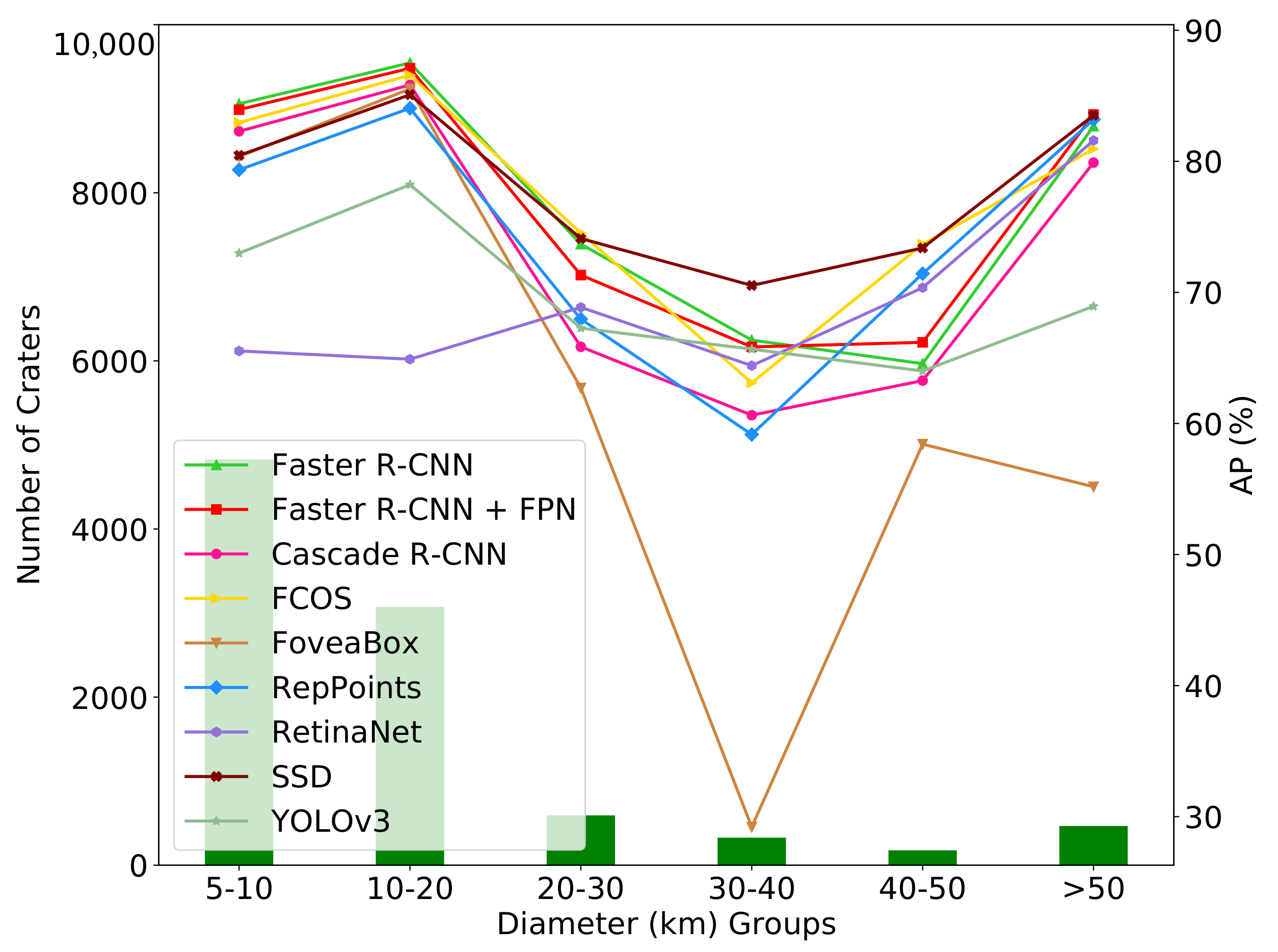
According to previous works [2,58], some researchers are more concerned with the distribution of lunar craters in a specific diameter range. Therefore, we conduct the performance evaluation of different models for lunar crater detection on different diameter groups of the test set. As shown in Table 2, we found that different models are good at detecting the craters in different diameter ranges. Faster R-CNN and Faster R-CNN + FPN achieve the superior performance for the detection of lunar craters with 5–20 km and ≥50 km diameters. FCOS gets the highest AP values when detecting lunar craters with 20–30 km and 40–50 km diameters. SSD has a more balanced detection performance than other models on all the diameter groups. We think that the reason of the performance differences among models is mainly due to the assignment strategy of the positive and negative samples, which involves the assignment of a specific set of anchor/point samples on different levels of features for the classification and regression tasks. For example, Faster R-CNN + FPN assigns three types of anchor boxes with different scales and aspect ratios to each output feature map of the FPN module, while SSD uses six or ten types of anchor boxes tiled on each feature map of the SSD-style pyramid module. How to design the optimal assignment is an open question. Figure 8 shows the variation of AP for the models on different diameter groups of the test set with the number of the GT craters on the training set. We observed that AP of most of models begins with a high value on the diameter groups of 5–10 km and 10–20 km, and then dramatically drops on the diameter groups of 20–30 km and 30–40 km, and finally raises on the diameter groups of 40–50 km and ≥50 km. It could be that the detection performance of the small and medium craters mainly depends on the number of the GT samples, and is worse when the samples are decreased on the diameter range of 5–40 km. With the improvement of resolution for the large craters, the corresponding samples provide easily recognizable information so that the performance of models is gradually improved on the large diameter groups of 40–50 km and ≥50 km.

4. Discussion

In this section, we discuss the practical application of the proposed workflow, and give an example method to demonstrate the performance advantage by comparing to a recent DEM-based CDA using CNN. To prove that the method can detect new lunar craters missed in the hand-labeled datasets, we develop a crater verification tool to manually validate the detection results and provide a revised confidence threshold in the detection stage. Furthermore, we show the visualization results to indicate that the detected craters (D < 50 km) are reasonable and can be used as a supplement to the hand-labeled datasets.

4.1. Lunar Crater Detection

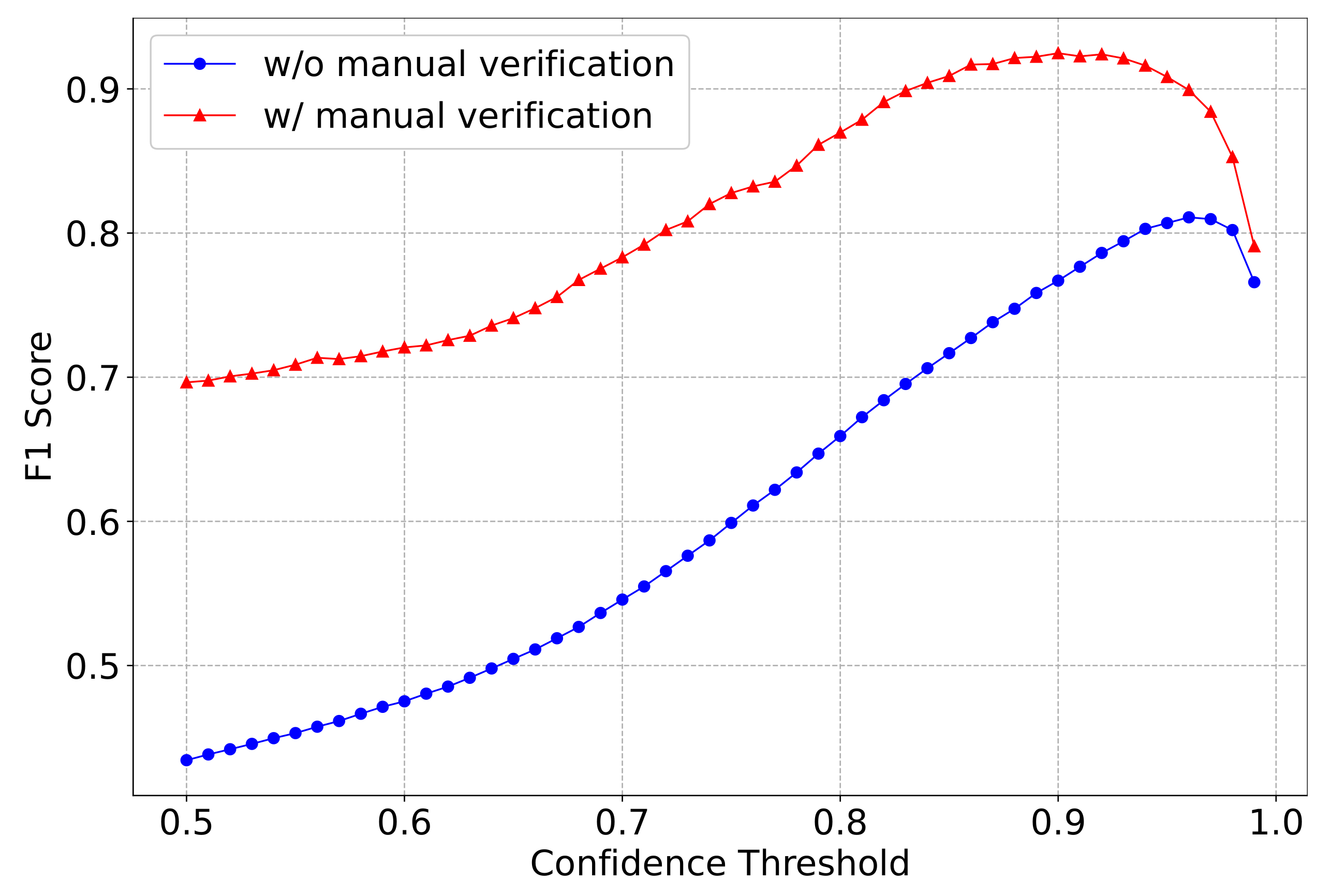
According to the benchmark results in Section 3.2, we find that our workflow with the Faster R-CNN + FPN model can obtain a much better overall performance for lunar crater detection. We use this model as an example to further analyze the effectiveness of our workflow in this section. To determine a set of detected craters, we need to use a specific confidence threshold for crater/non-crater classification. Here, we apply a discrete exhaustive search of confidence thresholds in a range from 0.5 to 1.0 on the validation set. The blue curve in Figure 9 shows that the confidence threshold of 0.96 leads to a highest F1 score. We compare the detection metrics of our method with DeepMoon [20], a classic deep learning approach for lunar crater detection on DEM data, and find that our method has lower recalls but much higher precisions on the validation set and test set, resulting in a better overall performance with the higher F1 scores (see Table 3). As the dataset we use only provides the annotated craters with a diameter ≥ 5 km, we also give the corresponding precision and F1 score for our detection results on the both sets, and prove the detection capacity of our method for the existing GT craters. In addition, we find that the fractional errors in latitude and radius of our method are similar to the results of DeepMoon, while the fractional longitude error we achieved has an obvious improvement.

4.2. Lunar Crater Verification

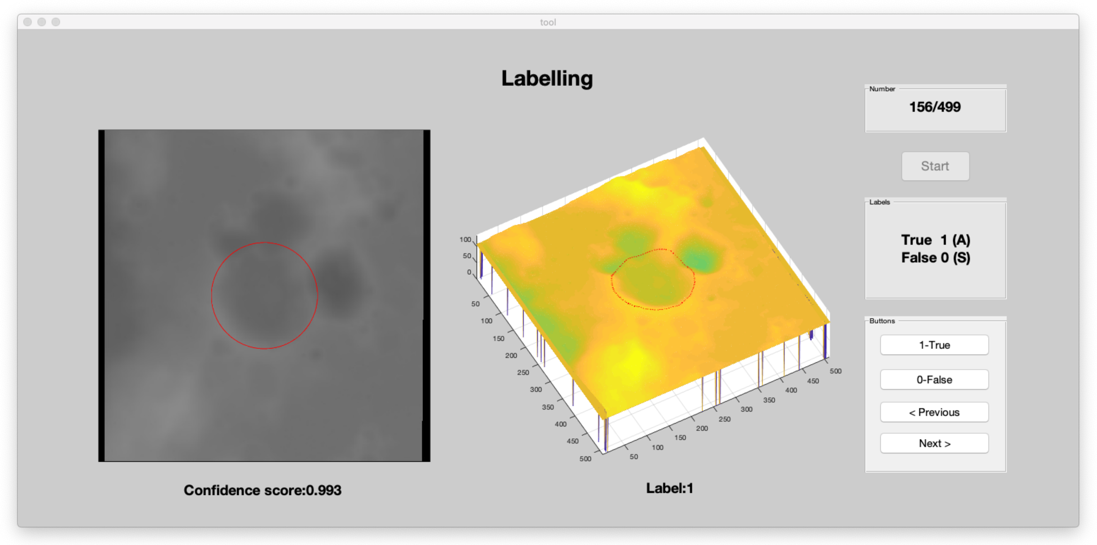
From the statistics of our detection results, there are 15,311 predicted craters with confidence score greater than 0.5, of which 10,991 are considered as FPs in the validation set. Since the current hand-labeled datasets include the incomplete GT craters, we have to manually validate the detection results and get a revised confidence threshold reflecting the real distribution of lunar craters. For this purpose, we develop an off-line crater verification tool as shown in Figure 10. The tool applies the orthographic projection and linear transformation operations for display preparation, and provides the two-dimensional and three-dimensional visualizations of each detected crater with the edge marked by a red circle. In addition, the tool also provides some simple buttons for the crater judgement and the annotation backtrack. In our work, we first sample 499 FP craters with the confidences covering the ranges from 0.5–0.6, 0.6–0.7, 0.7–0.8, 0.8–0.9, and 0.9–1.0 by using the same distribution proportion as the overall results. Then, these samples are independently verified and re-labeled by three scientists, and used to estimate the new TP craters in total. Finally, we re-calculate the precision and recall of our detection results by using the following formulas:
P r e c i s i o n n e w = N T P + N T P n e w N T P + N F P , R e c a l l n e w = N T P + N T P n e w N G T + N T P n e w .
The red curve in Figure 9 shows the variation of revised F1 score with confidence threshold on the validation set. We can see that all the F1 scores are improved obviously after the manual verification. It indicates that our method can identify lunar craters that were missed in previous hand-labeled datasets. In addition, our experimental results show that the confidence threshold of 0.90 is more reasonable for the lunar crater detection because it has an optimal F1 score in the crater validation on the lunar surface. Furthermore, we apply the new confidence threshold to manually validate 384 new detected samples from the test set, and estimate the true positive rate of new identified craters to be 83%, which leads to a consistent performance improvement with a F1 score of 0.93.

4.3. Visualization Results

The crater size-frequency distribution (CSFD) is a widely used technique to investigate the impact processes of the planetary surface. Previous works [2,59,60] show that the CSFD of the Moon follows a power law function, which is almost similar to the size-frequency distribution of asteroids in the main belt. Here we follow the works [20,21] and use the CSFD as a direct parameter to validate whether our automatic detection of craters over the lunar surface is plausible. As the asteroids from the main belt are considered as the impactor source forming the craters over the lunar surface, the CSFD from the automatic detection should follow the power law function even the efficiencies of crater detections for different size are different (see Table 2).
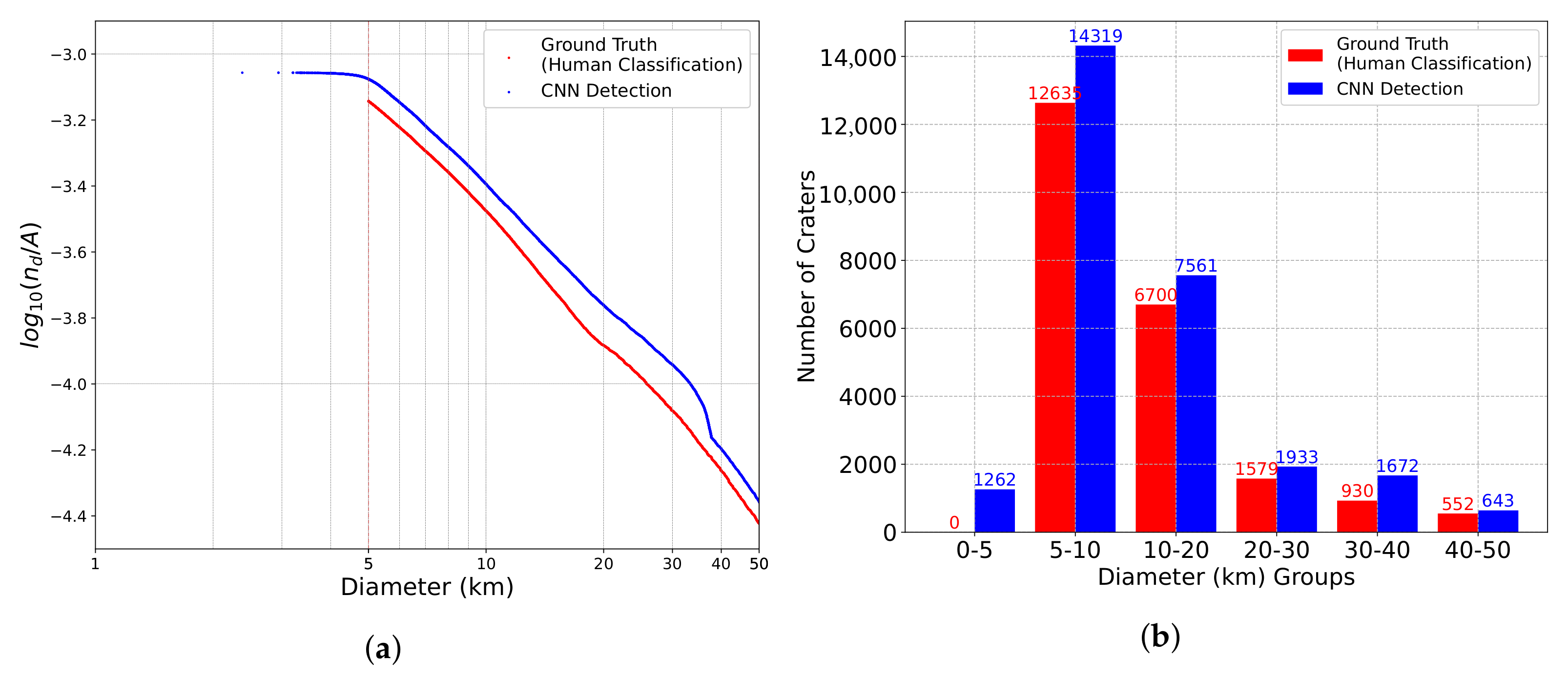
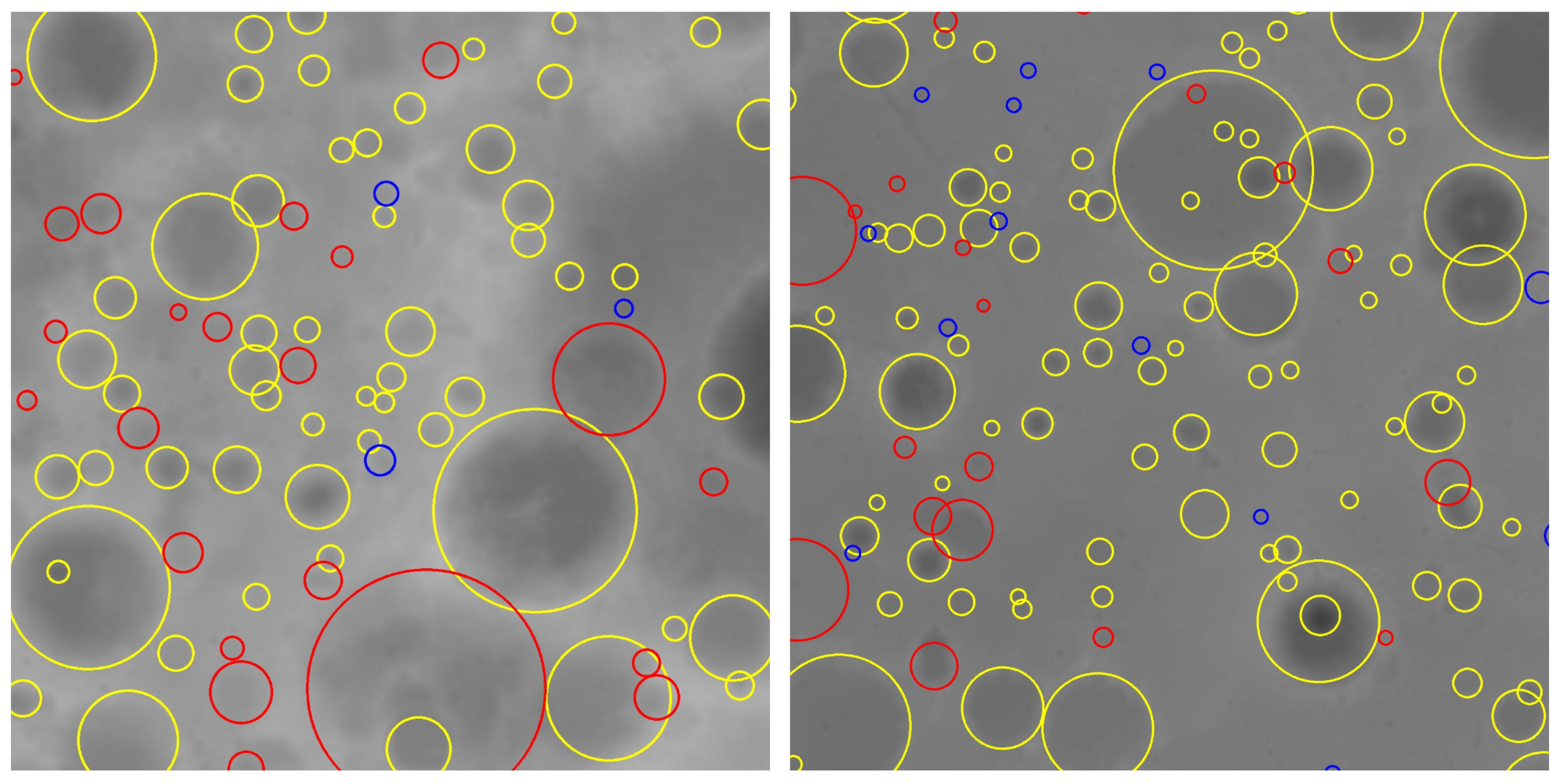
In Figure 11a, we show the CSFD of the craters detected by our proposed workflow with an example CNN model, while comparing with the CSFD of the GT craters obtained by human classification in the previous works [2,5]. We follow the recommendation in the work [61] and use the concerned surface area, A, to normalize the number of the craters over the Moon within the latitude range from 60 to 60 for a diameter between 1 and 50 km. We found that the CNN derived CSFD is systematically higher than the human derived CSFD, but they have a similar trend with a part of the same slopes. Combined with the size statistics of the craters in Figure 11b, it suggests that the CNN detection results include a larger number of craters than the hand-labeled results, while the new identified craters have the similar size distribution as the human identified craters. According to the manual verification in Section 4.2 and the previous works [20,21], which have pointed out that the GT craters are not complete, it reassures us that most of the new identified craters could be real. In Figure 12, we show two examples for our detection results, which include the matched craters, the newly identified craters and the undetected craters denoted by yellow circles, red circles and blue circles, respectively. Here, we regard a detected crater as the matched one of a GT crater when the IoU between them is larger than 0.5. We see that our method can detect most of GT craters with different diameters, and further identifies new craters that conform to the visual feature of a real crater on the DEM image. Although there are a few GT craters undetected by our method, which lead to a lower recall (see Table 3), our detection results can be used as a supplement of the previous hand-labeled datasets for the lunar research. In Table 4, we compare two existing lunar crater catalogs [2,5] with our extended lunar crater catalog by combining new identified craters with all the GT craters over the Moon within the latitude range from 60 to 60 .

5. Conclusions

In this work, we propose a complete and effective workflow using deep learning for lunar crater detection on the DEM data, which focuses on the detection of small craters (D < 50 km) over the lunar surface. The workflow is highly flexible to integrate various CNN-based detection models, and avoids a traditional two-stage pipeline processing by directly predicting the location and size of each crater. To reduce the gap between the existing DEM-based CDAs and the advanced methods for object detection, we build a new benchmark based on our workflow by conducting a thorough evaluation of three popular types of detection architectures with nine CNN models. In addition, we demonstrate a detailed example for the best practice of the proposed workflow, including the choice of a confidence threshold in the detection stage by developing a crater verification tool. Extended experiments show that our method has good performance since it effectively trades off the precision and recall of detected craters while identifying new craters missed in the hand-labeled datasets. In future work, we will apply our workflow to the detection of impact craters over other terrestrial planets besides the Moon, such as Mercury and Mars.

Author Contributions

Conceptualization, X.L., Z.Z. and Y.L.; methodology, X.L.; software, Z.Z.; validation, X.L., Z.Z. and X.X.; formal analysis, X.L., Z.Z. and X.Y.; investigation, X.Y. and T.L.; resources, X.J. and Y.L.; data curation, Z.Z. and X.J.; writing—original draft preparation, X.L. and Z.Z.; writing—review and editing, M.Z. and Y.L.; visualization, Z.Z. and X.X.; supervision, X.L.; project administration, Y.L.; funding acquisition, Y.L. All authors have read and agreed to the published version of the manuscript.

Funding

This research was funded by the Science and Technology Development Fund of Macau, grant number 0025/2019/AKP, 0010/2019/AFJ, 0004/2020/A1.

Institutional Review Board Statement

Not applicable.

Informed Consent Statement

Not applicable.

Data Availability Statement

The extended lunar crater catalog data is publicly available. This data can be found here: https://github.com/MUST-AI-Lab/DCDF-DEM, accessed on 15 December 2021.

Conflicts of Interest

The authors declare no conflict of interest.

References

  1. Wiesli, R.A.; Beard, B.L.; Taylor, L.A.; Johnson, C.M. Space weathering processes on airless bodies: Fe isotope fractionation in the lunar regolith. Earth Planet. Sci. Lett. 2003, 216, 457–465. [Google Scholar] [CrossRef]
  2. Head, J.W.; Fassett, C.I.; Kadish, S.J.; Smith, D.E.; Zuber, M.T.; Neumann, G.A.; Mazarico, E. Global distribution of large lunar craters: Implications for resurfacing and impactor populations. Science 2010, 329, 1504–1507. [Google Scholar] [CrossRef] [PubMed]
  3. Neukum, G.; Ivanov, B.A.; Hartmann, W.K. Cratering records in the inner solar system in relation to the lunar reference system. In Chronology and Evolution of Mars; Springer: Berlin/Heidelberg, Germany, 2001; pp. 55–86. [Google Scholar]
  4. Salih, A.L.; Schulte, P.; Grumpe, A.; Wöhler, C.; Hiesinger, H. Automatic crater detection and age estimation for mare regions on the lunar surface. In Proceedings of the 25th European Signal Processing Conference (EUSIPCO), Kos Island, Greece, 28 August–2 September 2017; pp. 518–522. [Google Scholar]
  5. Povilaitis, R.; Robinson, M.; Van der Bogert, C.; Hiesinger, H.; Meyer, H.; Ostrach, L. Crater density differences: Exploring regional resurfacing, secondary crater populations, and crater saturation equilibrium on the moon. Planet. Space Sci. 2018, 162, 41–51. [Google Scholar] [CrossRef]
  6. Leroy, B.; Medioni, G.; Johnson, E.; Matthies, L. Crater detection for autonomous landing on asteroids. Image Vis. Comput. 2001, 19, 787–792. [Google Scholar] [CrossRef]
  7. Kim, J.R.; Muller, J.P.; van Gasselt, S.; Morley, J.G.; Neukum, G. Automated crater detection, a new tool for Mars cartography and chronology. Photogramm. Eng. Remote Sens. 2005, 71, 1205–1217. [Google Scholar] [CrossRef] [Green Version]
  8. Sawabe, Y.; Matsunaga, T.; Rokugawa, S. Automated detection and classification of lunar craters using multiple approaches. Adv. Space Res. 2006, 37, 21–27. [Google Scholar] [CrossRef]
  9. Ding, M.; Cao, Y.; Wu, Q. Novel approach of crater detection by crater candidate region selection and matrix-pattern-oriented least squares support vector machine. Chin. J. Aeronaut. 2013, 26, 385–393. [Google Scholar] [CrossRef] [Green Version]
  10. Cohen, J.P.; Ding, W. Crater detection via genetic search methods to reduce image features. Adv. Space Res. 2014, 53, 1768–1782. [Google Scholar] [CrossRef] [Green Version]
  11. Salamuniccar, G.; Loncaric, S. Method for crater detection from martian digital topography data using gradient value/orientation, morphometry, vote analysis, slip tuning, and calibration. IEEE Trans. Geosci. Remote Sens. 2010, 48, 2317–2329. [Google Scholar] [CrossRef]
  12. Xie, Y.; Tang, G.; Yan, S.; Lin, H. Crater detection using the morphological characteristics of Chang’E-1 digital elevation models. IEEE Geosci. Remote Sens. Lett. 2013, 10, 885–889. [Google Scholar]
  13. Liu, D.; Chen, M.; Qian, K.; Lei, M.; Zhou, Y. Boundary detection of dispersal impact craters based on morphological characteristics using lunar digital elevation model. IEEE J. Sel. Top. Appl. Earth Obs. Remote Sens. 2017, 10, 5632–5646. [Google Scholar] [CrossRef]
  14. Chen, M.; Liu, D.; Qian, K.; Li, J.; Lei, M.; Zhou, Y. Lunar crater detection based on terrain analysis and mathematical morphology methods using digital elevation models. IEEE Trans. Geosci. Remote Sens. 2018, 56, 3681–3692. [Google Scholar] [CrossRef]
  15. Wang, Y.; Wu, B.; Xue, H.; Li, X.; Ma, J. An Improved Global Catalog of Lunar Impact Craters (≥1 km) with 3D Morphometric Information and Updates on Global Crater Analysis. J. Geophys. Res. Planets 2021, 126, e2020JE006728. [Google Scholar] [CrossRef]
  16. Di, K.; Li, W.; Yue, Z.; Sun, Y.; Liu, Y. A machine learning approach to crater detection from topographic data. Adv. Space Res. 2014, 54, 2419–2429. [Google Scholar] [CrossRef]
  17. Boukercha, A.; Al-Tameemi, A.; Grumpe, A.; Wöhler, C. Automatic Crater Recognition Using Machine Learning with Different Features and Their Combination. In Proceedings of the 45th Lunar and Planetary Science Conference (LPSC), The Woodlands, TX, USA, 17–21 March 2014; p. 2842. [Google Scholar]
  18. Palafox, L.; Alvarez, A.; Hamilton, C. Automated detection of impact craters and volcanic rootless cones in mars satellite imagery using convolutional neural networks and support vector machines. In Proceedings of the 46th Lunar and Planetary Science Conference (LPSC), The Woodlands, TX, USA, 16–20 March 2015; pp. 1–2. [Google Scholar]
  19. Emami, E.; Bebis, G.; Nefian, A.; Fong, T. Automatic crater detection using convex grouping and convolutional neural networks. In Proceedings of the 11th International Symposium on Visual Computing (ISVC), Las Vegas, NV, USA, 14–16 December 2015; pp. 213–224. [Google Scholar]
  20. Silburt, A.; Ali-Dib, M.; Zhu, C.; Jackson, A.; Valencia, D.; Kissin, Y.; Tamayo, D.; Menou, K. Lunar crater identification via deep learning. Icarus 2019, 317, 27–38. [Google Scholar] [CrossRef] [Green Version]
  21. Ali-Dib, M.; Menou, K.; Jackson, A.P.; Zhu, C.; Hammond, N. Automated crater shape retrieval using weakly-supervised deep learning. Icarus 2020, 345, 113749. [Google Scholar] [CrossRef] [Green Version]
  22. Krizhevsky, A.; Sutskever, I.; Hinton, G.E. Imagenet classification with deep convolutional neural networks. In Proceedings of the Advances in Neural Information Processing Systems (NIPS), Lake Tahoe, NV, USA, 3–8 December 2012; pp. 1097–1105. [Google Scholar]
  23. Long, J.; Shelhamer, E.; Darrell, T. Fully convolutional networks for semantic segmentation. In Proceedings of the 2015 IEEE Conference on Computer Vision and Pattern Recognition (CVPR), Boston, MA, USA, 7–12 June 2015; pp. 3431–3440. [Google Scholar]
  24. Ren, S.; He, K.; Girshick, R.; Sun, J. Faster r-cnn: Towards real-time object detection with region proposal networks. In Proceedings of the Advances in Neural Information Processing Systems (NIPS), Montreal, QC, Canada, 7–12 December 2015; pp. 91–99. [Google Scholar]
  25. Lowe, D.G. Distinctive image features from scale-invariant keypoints. Int. J. Comput. Vis. 2004, 60, 91–110. [Google Scholar] [CrossRef]
  26. Dalal, N.; Triggs, B. Histograms of oriented gradients for human detection. In Proceedings of the 2005 International Conference on Computer Vision Pattern Recognition (CVPR), San Diego, CA, USA, 20–26 June 2005; pp. 886–893. [Google Scholar]
  27. Cohen, J.P.; Lo, H.Z.; Lu, T.; Ding, W. Crater detection via convolutional neural networks. In Proceedings of the 47th Lunar and Planetary Science Conference (LPSC), The Woodlands, TX, USA, 21–25 March 2016; p. 1143. [Google Scholar]
  28. Wang, H.; Jiang, J.; Zhang, G. CraterIDNet: An End-to-End Fully Convolutional Neural Network for Crater Detection and Identification in Remotely Sensed Planetary Images. Remote Sens. 2018, 10, 1067. [Google Scholar] [CrossRef] [Green Version]
  29. Hashimoto, S.; Mori, K. Lunar crater detection based on grid partition using deep learning. In Proceedings of the 2019 IEEE 13th International Symposium on Applied Computational Intelligence and Informatics (SACI), Timisoara, Romania, 29–31 May 2019; pp. 75–80. [Google Scholar]
  30. Ronneberger, O.; Fischer, P.; Brox, T. U-net: Convolutional networks for biomedical image segmentation. In Proceedings of the 18th International Conference on Medical Image Computing and Computer-assisted Intervention (MICCAI), Munich, Germany, 5–9 October 2015; pp. 234–241. [Google Scholar]
  31. He, K.; Gkioxari, G.; Dollár, P.; Girshick, R. Mask r-cnn. In Proceedings of the 2017 IEEE International Conference on Computer Vision (ICCV), Venice, Italy, 22–29 October 2017; pp. 2961–2969. [Google Scholar]
  32. Jia, Y.; Wan, G.; Liu, L.; Wang, J.; Wu, Y.; Xue, N.; Wang, Y.; Yang, R. Split-Attention Networks with Self-Calibrated Convolution for Moon Impact Crater Detection from Multi-Source Data. Remote Sens. 2021, 13, 3193. [Google Scholar] [CrossRef]
  33. Wang, S.; Fan, Z.; Li, Z.; Zhang, H.; Wei, C. An Effective Lunar Crater Recognition Algorithm Based on Convolutional Neural Network. Remote Sens. 2020, 12, 2694. [Google Scholar] [CrossRef]
  34. Jia, Y.; Liu, L.; Zhang, C. Moon Impact Crater Detection Using Nested Attention Mechanism Based UNet++. IEEE Access 2021, 9, 44107–44116. [Google Scholar] [CrossRef]
  35. Wu, Y.; Wan, G.; Liu, L.; Wei, Z.; Wang, S. Intelligent Crater Detection on Planetary Surface Using Convolutional Neural Network. In Proceedings of the IEEE 5th Advanced Information Technology, Electronic and Automation Control Conference (IAEAC), Chongqing, China, 12–14 March 2021; pp. 1229–1234. [Google Scholar]
  36. Liu, W.; Anguelov, D.; Erhan, D.; Szegedy, C.; Reed, S.; Fu, C.Y.; Berg, A.C. Ssd: Single shot multibox detector. In Proceedings of the 14th European Conference on Computer Vision (ECCV), Amsterdam, The Netherlands, 8–16 October 2016; pp. 21–37. [Google Scholar]
  37. Lin, T.Y.; Dollár, P.; Girshick, R.; He, K.; Hariharan, B.; Belongie, S. Feature pyramid networks for object detection. In Proceedings of the 2017 IEEE Conference on Computer Vision and Pattern Recognition (CVPR), Honolulu, HI, USA, 21–26 July 2017; pp. 2117–2125. [Google Scholar]
  38. Tian, Z.; Shen, C.; Chen, H.; He, T. Fcos: Fully convolutional one-stage object detection. In Proceedings of the 2019 IEEE/CVF International Conference on Computer Vision (ICCV), Seoul, Korea, 27–28 October 2019; pp. 9627–9636. [Google Scholar]
  39. Cai, Z.; Vasconcelos, N. Cascade r-cnn: Delving into high quality object detection. In Proceedings of the 2018 IEEE/CVF Conference on Computer Vision and Pattern Recognition (CVPR), Salt Lake City, UT, USA, 18–23 June 2018; pp. 6154–6162. [Google Scholar]
  40. Redmon, J.; Farhadi, A. Yolov3: An incremental improvement. arXiv 2018, arXiv:1804.02767. [Google Scholar]
  41. Lin, T.Y.; Goyal, P.; Girshick, R.; He, K.; Dollár, P. Focal loss for dense object detection. In Proceedings of the 2017 IEEE International Conference on Computer Vision (ICCV), Venice, Italy, 22–29 October 2017; pp. 2980–2988. [Google Scholar]
  42. Kong, T.; Sun, F.; Liu, H.; Jiang, Y.; Li, L.; Shi, J. Foveabox: Beyound anchor-based object detection. IEEE Trans. Image Process. 2020, 29, 7389–7398. [Google Scholar] [CrossRef]
  43. Yang, Z.; Liu, S.; Hu, H.; Wang, L.; Lin, S. Reppoints: Point set representation for object detection. In Proceedings of the 2019 IEEE/CVF International Conference on Computer Vision (ICCV), Seoul, Korea, 27–28 October 2019; pp. 9657–9666. [Google Scholar]
  44. Barker, M.; Mazarico, E.; Neumann, G.; Zuber, M.; Haruyama, J.; Smith, D. A new lunar digital elevation model from the Lunar Orbiter Laser Altimeter and SELENE Terrain Camera. Icarus 2016, 273, 346–355. [Google Scholar] [CrossRef] [Green Version]
  45. Scholten, F.; Oberst, J.; Matz, K.D.; Roatsch, T.; Wählisch, M.; Speyerer, E.; Robinson, M. GLD100: The near-global lunar 100 m raster DTM from LROC WAC stereo image data. J. Geophys. Res. Planets 2012, 117, E00H17. [Google Scholar] [CrossRef] [Green Version]
  46. Girshick, R. Fast r-cnn. In Proceedings of the 2015 IEEE International Conference on Computer Vision (ICCV), Santiago, Chile, 7–13 December 2015; pp. 1440–1448. [Google Scholar]
  47. Met Office. Cartopy: A Cartographic Python Library with a Matplotlib Interface; Met Office: Exeter, UK, 2010. [Google Scholar]
  48. Deng, J.; Dong, W.; Socher, R.; Li, L.J.; Li, K.; Fei-Fei, L. Imagenet: A large-scale hierarchical image database. In Proceedings of the 2009 IEEE Conference on Computer Vision and Pattern Recognition (CVPR), Miami, FL, USA, 20–25 June 2009; pp. 248–255. [Google Scholar]
  49. Zeiler, M.D.; Fergus, R. Visualizing and understanding convolutional networks. In Proceedings of the 13th European Conference on Computer Vision (ECCV), Zurich, Switzerland, 6–12 September 2014; pp. 818–833. [Google Scholar]
  50. Lin, X.; Liang, Y.; Wan, J.; Lin, C.; Li, S.Z. Region-Based Context Enhanced Network for Robust Multiple Face Alignment. IEEE Trans. Multimedia 2019, 21, 3053–3067. [Google Scholar] [CrossRef]
  51. He, K.; Zhang, X.; Ren, S.; Sun, J. Deep residual learning for image recognition. In Proceedings of the 2016 IEEE Conference on Computer Vision and Pattern Recognition (CVPR), Las Vegas, NV, USA, 27–30 June 2016; pp. 770–778. [Google Scholar]
  52. Eslami, M.E.S.A.; Van Gool, L.; Williams, C.K.; Winn, J.; Zisserman, A. The pascal visual object classes challenge: A retrospective. Int. J. Comput. Vis. 2015, 111, 98–137. [Google Scholar]
  53. Lin, T.Y.; Maire, M.; Belongie, S.; Hays, J.; Perona, P.; Ramanan, D.; Dollár, P.; Zitnick, C.L. Microsoft coco: Common objects in context. In Proceedings of the 13th European Conference on Computer Vision (ECCV), Zurich, Switzerland, 6–12 September 2014; pp. 740–755. [Google Scholar]
  54. Simonyan, K.; Zisserman, A. Very Deep Convolutional Networks for Large-Scale Image Recognition. In Proceedings of the 3rd International Conference on Learning Representations (ICLR), San Diego, CA, USA, 7–9 May 2015. [Google Scholar]
  55. Liu, W.; Liao, S.; Ren, W.; Hu, W.; Yu, Y. High-level semantic feature detection: A new perspective for pedestrian detection. In Proceedings of the 2019 IEEE/CVF Conference on Computer Vision and Pattern Recognition (CVPR), Long Beach, CA, USA, 15–20 June 2019; pp. 5187–5196. [Google Scholar]
  56. Yu, J.; Jiang, Y.; Wang, Z.; Cao, Z.; Huang, T. Unitbox: An advanced object detection network. In Proceedings of the 24th ACM International Conference on Multimedia (MM), New York, NY, USA, 15–19 October 2016; pp. 516–520. [Google Scholar]
  57. Girshick, R.; Donahue, J.; Darrell, T.; Malik, J. Rich feature hierarchies for accurate object detection and semantic segmentation. In Proceedings of the 2014 IEEE Conference on Computer Vision and Pattern Recognition (CVPR), Columbus, OH, USA, 23–28 June 2014; pp. 580–587. [Google Scholar]
  58. Ivanov, B. Size-frequency distribution of small lunar craters: Widening with degradation and crater lifetime. Sol. Syst. Res. 2018, 52, 1–25. [Google Scholar] [CrossRef]
  59. Bottke, W.F.; Norman, M.D. The late heavy bombardment. Annu. Rev. Earth Planet. Sci. 2017, 45, 619–647. [Google Scholar] [CrossRef] [Green Version]
  60. Bottke, W. Dynamical Evolution and Bombardment of the Early Solar System: A Few Highlights of the Last 50 Years. In Proceedings of the 50th Lunar and Planetary Science Conference (LPSC), The Woodlands, TX, USA, 18–22 March 2019; p. 1545. [Google Scholar]
  61. Crater Analysis Techniques Working Group. Standard techniques for presentation and analysis of crater size-frequency data. Icarus 1979, 37, 467–474. [Google Scholar] [CrossRef] [Green Version]
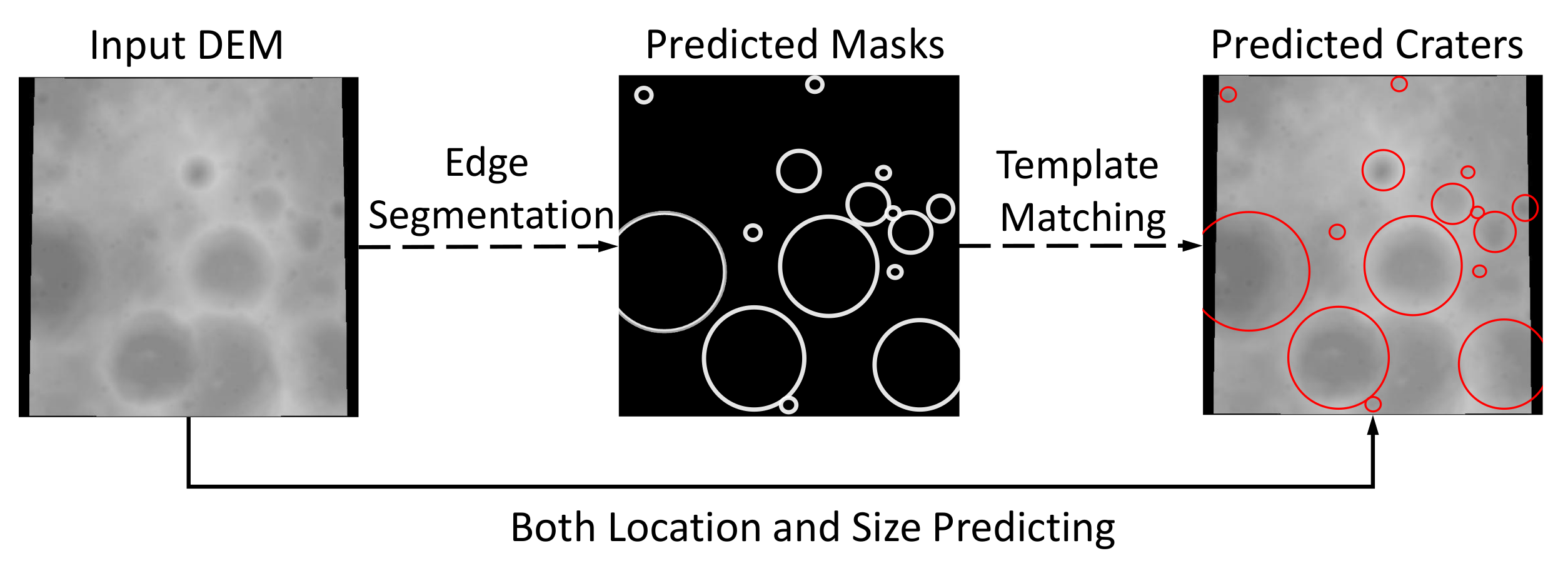
Figure 1. Comparison of the two-stage pipeline (dotted line) and the end-to-end pipeline (solid line) for lunar crater detection on the DEM data.
Remotesensing 14 00621 g001
Figure 2. A multi-scale grid cropping strategy applied to the lunar DEM image.
Remotesensing 14 00621 g002
Figure 3. Architecture of the region-based detection network for lunar crater detection.
Remotesensing 14 00621 g003
Figure 4. Architecture of the anchor-based detection network for lunar crater detection.
Remotesensing 14 00621 g004
Figure 5. Architecture of the point-based detection network for lunar crater detection.
Remotesensing 14 00621 g005
Figure 6. Variation of Average precision (AP) for nine CNN models with the IoU threshold on the validation (a) and test (b) sets.
Remotesensing 14 00621 g006
Figure 7. Precision-recall (P-R) curves of nine CNN models with different IoU thresholds on the validation (ac) and test (df) sets.
Remotesensing 14 00621 g007
Figure 8. Variation of Average precision (AP) for nine CNN models on different diameter groups of the test set with the number of the ground-truth (GT) craters on the training set.
Remotesensing 14 00621 g008
Figure 9. Variation of F1 score with confidence threshold for our workflow using Faster R-CNN + FPN on the validation set. The red and blue curves denote the results with (w/) and without (w/o) manual verification of detected craters, respectively.
Remotesensing 14 00621 g009
Figure 10. Graphical user interface of our crater verification tool.
Remotesensing 14 00621 g010
Figure 11. Cumulative size-frequency distribution (CSFD) (a) and size statistics (b) of the craters detected by CNN (blue) and obtained by human classification (red) with a diameter between 1 and 50 km.
Remotesensing 14 00621 g011
Figure 12. Example results of our method on the test set. Yellow circles represent detected craters that were successfully matched to the ground-truth targets. Red circles are newly identified craters that are not labeled on the current datasets. Blue circles represent the ground-truth craters undetected by our method.
Remotesensing 14 00621 g012
Table 1. Average precision (AP) of nine CNN models on the validation and test sets with their parameters and GFLOPs. IoU thr is the IoU threshold during model evaluation.
MethodAP↑ (IoU thr = 0.5)AP↑ (IoU thr = 0.6)AP↑ (IoU thr = 0.7)ParametersGFLOPs
ValidationTestValidationTestValidationTest
Faster R-CNN86.04%86.38%81.80%80.70%72.74%68.79%33.57 M760.86
Faster R-CNN + FPN86.01%87.02%80.92%80.70%70.58%67.94%41.53 M63.65
Cascade R-CNN84.76%84.98%78.36%77.31%66.23%64.37%69.17 M91.29
SSD85.08%84.61%79.02%78.28%69.42%66.20%36.04 M98.81
RetinaNet68.97%66.11%65.72%61.76%58.37%53.43%37.74 M61.22
YOLOv378.53%77.73%71.15%70.46%57.26%54.34%61.95 M50.06
FoveaBox73.94%76.02%67.24%66.73%55.60%54.86%36.19 M52.77
FCOS82.74%85.22%78.52%80.22%70.77%71.18%32.02 M51.32
RepPoints82.60%82.83%77.06%75.76%65.79%64.37%36.62 M48.66
Table 2. Average precision (AP) of nine CNN models on different diameter groups of the test set.
MethodAP↑ (IoU Threshold = 0.5)
5–10 km10–20 km20–30 km30–40 km40–50 km≥50 kmTotal
Faster R-CNN84.39%87.51%73.68%66.36%64.56%82.68%86.38%
Faster R-CNN + FPN83.94%87.10%71.32%65.84%66.19%83.57%87.02%
Cascade R-CNN82.29%85.83%65.85%60.63%63.27%79.90%84.98%
SSD80.45%85.08%74.11%70.53%73.39%83.51%84.61%
RetinaNet65.53%64.90%68.86%64.41%70.36%81.59%66.11%
YOLOv372.99%78.22%67.27%65.67%64.00%68.94%77.73%
FoveaBox80.36%85.53%62.71%29.21%58.42%55.17%76.02%
FCOS82.96%86.57%74.53%63.10%73.67%80.95%85.22%
RepPoints79.35%84.05%67.96%59.16%71.43%83.19%82.83%
Table 3. Detection metrics of the DeepMoon method and our workflow using Faster R-CNN + FPN on the validation and test sets.
Accuracy MetricDeepMoonOur Method
ValidationTestValidationTest
Recall↑92%92%81.20%79.39%
Precision↑53%56%80.99%82.97%
Precision(diameter ≥ 5 km)↑--90.67%91.61%
F1 score↑0.670.690.810.81
F1 score(diameter ≥ 5 km)↑--0.860.85
Fractional longitude error↓13%11%6.19%7.33%
Fractional latitude error↓10%9%9.39%9.25%
Fractional radius error↓6%7%6.05%6.76%
Table 4. Comparison of two existing lunar crater catalogs and our extended lunar crater catalog for different diameter ranges over the Moon within the latitude range from 60 to 60 .
Number of Lunar Craters
Diameter RangeHead et al. [2]Povilaitis et al. [5]Ours
1–5 km--991
5–20 km-19,33524,186
≥20 km4301-6429
Total430119,33531,606
Publisher’s Note: MDPI stays neutral with regard to jurisdictional claims in published maps and institutional affiliations.