Article

Dynamics of Mixing Layer Height and Homogeneity from Ceilometer-Measured Aerosol Profiles and Correlation to Ground Level PM2.5 in New York City

1
Optical Remote Sensing Laboratory, The City College of New York, New York, NY 10031, USA
2
NOAA—Cooperative Science Center for Earth System Sciences and Remote Sensing Technologies, New York, NY 10031, USA
*
Author to whom correspondence should be addressed.
Remote Sens. 2022, 14(24), 6370; https://doi.org/10.3390/rs14246370
Submission received: 20 October 2022 / Revised: 8 December 2022 / Accepted: 12 December 2022 / Published: 16 December 2022
(This article belongs to the Section Atmospheric Remote Sensing)

Abstract

:
Observations of mixing layer height (MLH), its dynamics and the extent of homogeneity of the mixing layer are important in the study of air pollution as well as meteorological and air quality model validation. They can contribute to improvements in the application of satellite aerosol optical depth (AOD) products to ground fine particulate matter (PM2.5) estimation that can potentially provide synoptic-scale monitoring of fine particulate matter. Ceilometers have shown great potential for continuous monitoring of MLH and aerosol profiles within the boundary layer. In this study, we report an automated quality control/quality assurance (QC/QA) method that improves the consistency of MLH retrievals from ceilometer measurements and present measurements of MLH variation in New York City (NYC) as observed by ceilometers in summer and winter seasons. Distinct issues due to SNR and quality of overlap correction are addressed within the QC/QA method. We also analyze the diurnal and seasonal correlations between ceilometer-attenuated backscatter and ground-level PM2.5 as a function of height, time of day, and season, to shed light on the homogeneity of aerosol vertical mixing within the MLH, as well as the correlation between aerosol optical properties and PM2.5. The results show that the overall correlation in summer is better than in winter. This correlation decreases with increasing height but the degradation is less severe in summer than in winter, which is qualitatively consistent with urban heating models of convective mixing. However, no significant diurnal variation of the correlation coefficient was observed for both seasons. We also found that the linear regression slope between ceilometer-attenuated backscatter coefficients and ground PM2.5 shows seasonal variation, which can be partially explained by the difference in aerosol size distribution and aerosol species between summer and winter. Finally, we investigated the homogeneity of aerosol vertical distribution within the mixing layer (ML) during the daytime. The results indicate that the aerosols are well-mixed within the lower part of ML up to 500 m.

1. Introduction

Air quality is of great concern due to its significant impact on the environment and human health. PM2.5, which refers to fine particulate matter with a diameter less than or equal to 2.5 μm, is a major urban air pollutant. Long-term exposure to PM2.5 can result in various respiratory and cardiovascular diseases, such as myocardial infarction, cardiac arrhythmia, and ischemic stroke [1,2]. In the New York City (NYC) metropolitan area, PM2.5 pollution contributes to more than 3000 deaths, 2000 hospital admissions for lung and heart conditions, and approximately 6000 emergency department visits for asthma each year [3]. The major sources of PM2.5 in NYC include traffic emissions, power plants, industrial activities and biomass burning [4]. Continuous monitoring of PM2.5 is important for improving air quality and to protect public health.
Since ground PM2.5 measurements are often limited by their sparse spatial coverage, many efforts have been made to estimate ground-level PM2.5 using satellite aerosol optical depth (AOD), providing supplemental information on PM2.5 concentrations. As satellite-derived AOD reflects the total amount of aerosols within a column of atmosphere, the relationship between surface PM2.5 and AOD also depends on the mixing layer height (MLH). Due to the net effect of capping inversion, mechanical turbulence, and free convection, most aerosols that include PM2.5 are trapped and dispersed within the mixing layer (ML) [5,6]. MLH serves as the depth of the volume where total PM2.5 is dispersed, resulting in a basic anti-correlation with the surface pollution [7,8,9,10]. Zhang and Li [11] established a remote-sensing formula for dry PM2.5 mass concentration near the ground, suggesting that satellite-measured AOD needs to be divided by MLH to better represent the surface PM2.5. Yang et al. [12] observed an enhanced correlation between surface PM2.5 and AOD after applying the vertical correction to AOD using MLH. Although MLH is a crucial parameter for PM2.5 estimation using AOD, this model is based on the assumption that aerosols are uniformly distributed within the ML, which may not always be valid. Variations in aerosol vertical distribution, aerosol species and size can influence the AOD-PM2.5 relationship, which results in a seasonal bias of satellite-derived PM2.5. For example, Liu et al. [13,14] developed a multivariable regression model to predict ground PM2.5 using satellite AOD. They found that the mixing layer height (MLH), relative humidity (RH), seasonal variation in the aerosol type and meteorological conditions can change the AOD-PM2.5 relationship. Observations of aerosol composition, particle size distribution, and vertical profiles can help to further improve the model. Van Donkelaar et al. [15] estimated seasonal PM2.5 in the U.S. and global annual PM2.5 distribution using satellite AOD. The results showed that the variation in the aerosol vertical profile has a critical impact on the PM2.5 prediction accuracy. Later, Van Donkelaar et al. [16] evaluated the impact of aerosol vertical profiles on the AOD-PM2.5 relationship by comparing GOES-CHEM model-simulated aerosol vertical profiles with Cloud-Aerosol Lidar with Orthogonal Polarization (CALIOP)-retrieved aerosol vertical profiles, indicating an underestimation of aerosol extinction in the GOES-CHEM model in the studied regions. Central Africa, Brazil, the eastern parts of Canada, northeastern America, and northern Europe exhibit increased error caused by the discrepancy of CALIOP-retrieved- and model-simulated aerosol profiles. Zheng et al. [17] stated that the aerosol vertical structure exhibits remarkable seasonal change, which contributes greatly to the AOD-PM2.5 relationship. Therefore, observations of MLH dynamics and a better understanding of the seasonal and spatial variations in aerosol vertical distribution, with a focus on the homogeneity of aerosols within the ML, are vital to improve the satellite-derived PM2.5 predictive approach.
Although originally designed for detecting cloud base height, ceilometers can be used to retrieve the MLH [18,19,20,21,22]. Considering their 24-h/7-day continuous observation capacity, eye-safe laser transmitting power, low cost and compact design, and easy maintenance, ceilometers are very suitable for deployment in a network for real-time or near real-time MLH observations for the validation and improvement of weather and air quality model forecasts. For example, the National Weather Service deploys ceilometers at different geographical regions in the United States to evaluate the ceilometer MLH detection capacity [23]. The Unified Ceilometer Network provides real-time hourly MLHs across the participating monitor sites for weather and air quality applications (https://www.ucn-portal.org, accessed on 25 November 2022).
Different methods for MLH estimation have been developed using lidar/ceilometer-attenuated backscatter coefficients, including the gradient method [18,21,24], the variance method [25,26], the wavelet covariance transform (WCT) method [19,27,28,29], and the ideal backscatter profile method [20,21,30]. Software provided by the ceilometer manufacturers can calculate aerosol layer heights (ALHs) for certain types of ceilometers; however, it usually remains for users to determine which one is the true MLH. In this case, it is necessary to develop additional quality control processes for the original ALH product [31,32] to obtain quality-assured MLH. Given the variety of ceilometer types and MLH detection methods, it is desirable to have a quantitative evaluation of MLH detection abilities across different ceilometers.
In addition to MLH detection, ceilometers can measure the attenuated backscatter profile which can represent the aerosol vertical distribution [33,34,35,36]. In particular, since the incomplete overlap range of ceilometers is usually shorter than a lidar system, the near-surface attenuated backscatter coefficient may serve as a proxy for surface PM2.5. Li et al. [37] incorporated ceilometer near-surface backscatter, Angstrom exponents, and temperature in their AOD-PM2.5 prediction model, significantly improving model accuracy, with the surface backscatter coefficient being the most important factor. The near-surface aerosol vertical distribution is usually difficult to obtain, yet is important, as most pollutants concentrate near the surface and directly affect human health. In this regard, ceilometer backscatter profiles can provide supplementary information even though they do not characterize aerosol types since ceilometers operate at a single wavelength. Nonetheless, studies assessing the correlation between PM2.5 and near-surface backscatter, and the factors that can influence their correlations, are still rare. Therefore, a major purpose of this work is to quantify the correlation between ceilometer backscatter and ground PM2.5 concentrations within the ML and to determine how the correlation may change vertically, diurnally, and seasonally, as well as to assess the aerosol vertical mixing using ceilometer backscatter profiles, which can ultimately improve air quality models and AOD-PM2.5 estimations.
In this paper, we first focus on the MLH optimal determination of two types of ceilometers which are widely used: Vaisala CL51 and Lufft CHM15k. A QC/QA algorithm was developed and applied to the ceilometers’ original ALH in order to obtain reliable MLH results. Then validation of MLH was carried out by inter-comparison across both of the ceilometer-optimized MLHs and the lidar-derived MLHs. Following this, the seasonal and diurnal variation of MLHs during 2015–2019 was characterized. Next, we investigated the correlation of the attenuated backscatter coefficients of Vaisala CL51 and Lufft CHM15k with lidar-retrieved aerosol backscatter. A comprehensive correlation study of ground-level PM2.5 and ceilometer-attenuated backscatter coefficients is presented in term of their seasonal and altitude dependencies. Last, we briefly discussed the seasonal and diurnal characteristics of aerosol vertical distribution using ceilometer-attenuated backscatter coefficients. The paper is organized as follows: Section 2 describes the instruments used and the methodology. In Section 3, we present the detailed results and discussion. The main conclusions are presented in Section 4.

2. Materials and Methods

2.1. Instruments

For this study, a Vaisala CL51 ceilometer, a Lufft CHM15k ceilometer, and a three-wavelength Elastic–Raman lidar were deployed on the roof of the Engineering School of the City College of New York (CCNY, 40.821°N, 73.948°W, altitude: 100 m). The distance between these three instruments was 5–10 m, far enough to avoid signal interference but close enough to collect data from the same atmospheric volume. A CIMEL sun-photometer operated by the AErosol RObotic NETwork (AERONET: https://aeronet.gsfc.nasa.gov/new_web/index.html, accessed on 25 November 2022) at the CCNY site measured AOD (at eight wavelengths 340–1640 nm), Angstrom exponent, and provided other aerosol products (aerosol volume size distribution, refractive index, single-scattering-albedo and others) [38,39]. About 220 m away was a surface air-quality-monitoring station operated by the New York State Department of Environment Conservation (NYSDEC), collecting PM2.5, ozone, and carbon monoxide concentration data with a temporal resolution of 1 min. There was also an automatic weather station, which provided meteorological observations, including atmospheric pressure, relative humidity, temperature, wind direction, wind speed, rain rate, and total rain accumulation at 5 min temporal resolution. The CCNY lidar system is a three wavelength Elastic-Raman lidar (355–532–1064 nm) which provides aerosol, water vapor and cloud measurements [40]. The temporal resolution of the raw profile is 1 min and its spatial resolution is 3.75 m. The lidar is primarily operated during the daytime and under appropriate weather conditions. The aerosol backscatter coefficients at 532–1064 nm were retrieved from the elastic scattering signals using the Fernald–Klett method [41,42], while a WCT method was used to estimate the MLH [22]. The Vaisala CL51 ceilometer uses an InGaAs diode laser operating at a wavelength of 910 ± 10 nm (25 °C, repetition rate: 6.5 kHz). The manufacturer provides an overlap correction embedded in every CL51 ceilometer to obtain theoretical results from the surface. The measurement range is 0–15 km. For the raw signal, the height resolution is 10 m and the time resolution is 16 s. The CL51 ceilometer collected data from March 2015 to February 2019, making 24 h observations automatically under all weather conditions. The Lufft CHM15k employs a diode-pumped Nd: YAG solid-state laser at 1064 nm with a spectral width of 1 nm. Given the biaxial optical design, the CHM15k starts to receive useful signals from 180 m and its full overlap range is around 1.5 km [33,43,44]. The overlap function is provided by the vendor for each ceilometer. The maximum measuring range is 15 km. The temporal/spatial resolution of a raw signal profile is 15 s/15 m. The Lufft CHM15k ceilometer was installed on October 2018 and has been making 24 h observations under all weather conditions since then. The key specifications of the lidar and ceilometers are shown in Table 1.

2.2. Quality Assurance of the MLH Determination by Ceilometers

The Vaisala Boundary Layer View (BL-View) is the manufacturer’s software that can analyze the MLHs for Vaisala CL31 and CL51 ceilometers. Its primary data products are ALH and cloudbase height (CBH) [45]. The Lufft CHM15k also detects up to three ALHs using the gradient signatures.
Although both ceilometers provide ALHs as MLH candidates, it remains for users to determine which layer height is the MLH. In many cases, the lowest aerosol layer retrieval coincides with the MLH, but the reliability of MLH products depends on the atmospheric and surface conditions. When MLH is prominent, different MLH retrieval methods with different ceilometers can attribute the same MLHs. However, when the MLH is not clearly defined or multiple aerosol layers occur due to local emission, a residual layer, or smoke plume transport from other places, different MLH algorithms may pick up different layer heights depending on the internal threshold setting, signal smooth method and SNR. Hence, in order to optimize the MLH estimate from the ceilometer ALH product, we developed a QC/QA method to remove the spurious MLHs. The criteria of QC/QA are: (i) lowest detectable ALHs are set to be the primary MLHs; (ii) discard the ALHs when precipitation, fog (or dense haze) or low cloud (<3 km) appears within a 3 min sliding window; (iii) MLHs are confined by certain limits (min. and max.) characterized by long-term seasonal statistical results; and (iv) MLHs vary in a continuous manner. Based on these criteria, we filtered out the spurious MLHs and obtained the 10-minute averaged QC/QA processed MLHs. The details of the QC/QA procedure is provided in Appendix A.1.
In alignment with the MLH analysis, the attenuated backscatter coefficients and CBHs from the ceilometer observations were averaged every 10 min. The time-averaged attenuated backscatter coefficient profile was then smoothed over the vertical range with a 50 m running mean window. Apart from the QC/QA process, we evaluated the sky condition to assure the MLH data quality for the ceilometer comparison study. Specifically, we initiated a sky condition quality flag for each attenuated backscatter coefficient profile (10-minute resolution). If the average attenuated backscatter coefficient below 500 m was greater than the threshold, which indicated rain, fog, or dust on the lens, the corresponding sky condition quality flag was set to one. If the duration of the poor sky condition was more than 3 h in a day, then the data for this day were not considered for the MLH validation. If the poor sky condition flag duration was less than 3 h, the partial data were processed.
In addition, we used a qualitatively different WCT method to estimate the MLHs from CCNY-lidar measurements [22]. This method was used to retrieve MLHs from CL51 data before June 2018 as the BL-View software was not yet available. The long-term MLHs of the CL51 ceilometer from March 2015 to February 2019 were used to evaluate the seasonal and diurnal variation of MLH in the NYC urban area.

3. Results and Discussion

3.1. MLH Detection, Validation and Seasonal Variation

An example of the QC/QA process applied to both ceilometer measurements on 4 February 2019 is shown in Figure 1a,b. The green symbols indicate the 16 s resolution MLHs determined by the lowest ALHs and the red crosses are spurious MLHs detected by the QC/QA process. The black symbols represent the quality-assured 10 min resolution MLHs. Generally, the QC/QA process can effectively remove the outliers, which are discontinuous over time. However, greater discrepancies between MLHs retrieved by the two ceilometers were observed before sunrise and after sunset. In particular, when the MLH was shallow and multiple aerosol layers occuredr, the CHM15k tended to pick the aloft ALH, while the CL51 selected the gradient at a lower level. This discrepancy was mainly due to the longer full-overlap range of the CHM15k, as well as different signal-smoothing methods and internal threshold settings of the two ceilometer systems to determine ALHs.
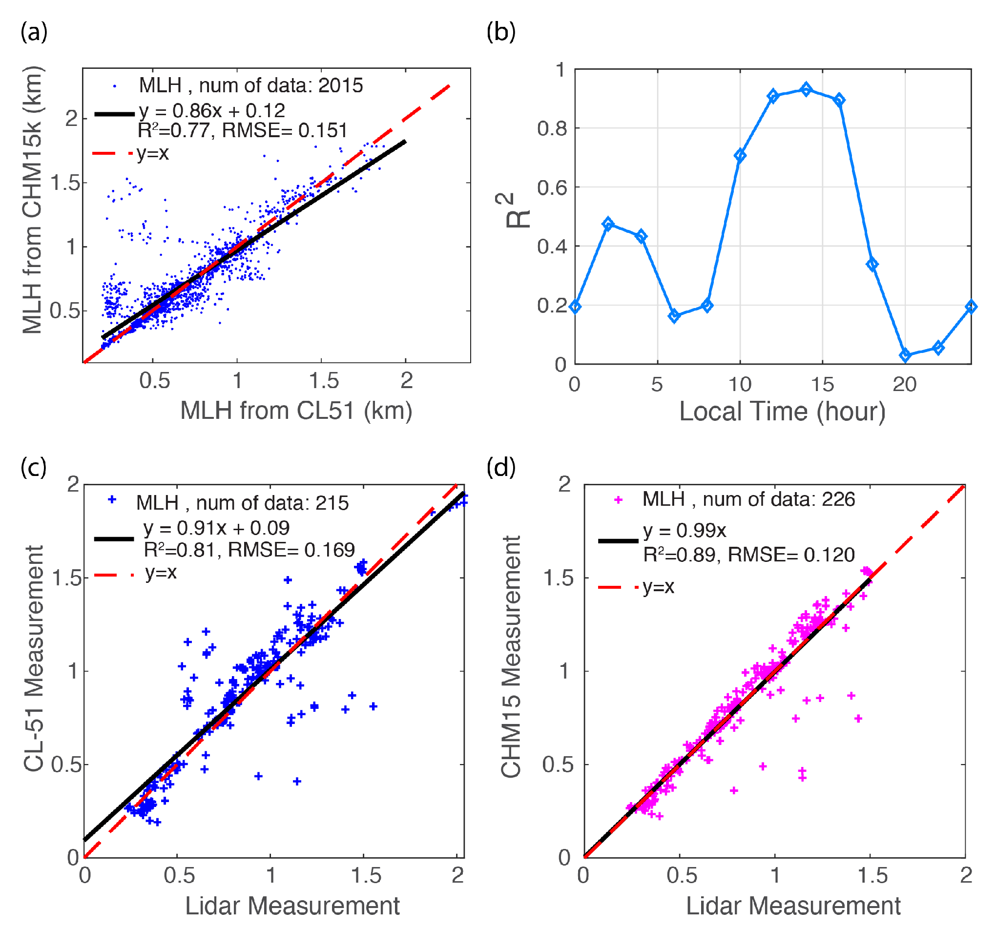
Next, we compared more than 2000 data points of the QC/QA processed MLHs from the two ceilometers on 28 clear sky days from 30 October 2018 to 15 February 2019. Due to the limitation stemming from the longer overlap function of CHM15k, we only chose the MLHs that were above 200 m for both ceilometers and their correlation analysis is shown in Figure 2. Before the QC/QA process, the correlation of MLHs determined by the lowest ALH candidates of two ceilometers was very poor ( R 2 = 0.1, not shown). After the QC/QA process, the correlation between the MLHs of the two ceilometers significantly improved, with correlation coefficient R 2 = 0.77, root mean square error (RMSE) = 0.151, and linear regression slope = 0.86 (Figure 2a). Figure 2b shows the diurnal characteristics of the correlation coefficient R 2 between the MLHs retrieved from the two ceilometers. Each data point corresponds to the R 2 of MLHs within a 2 h duration. A strong correlation occurred between 10:00 and 16:00 (local time) when the aerosols were more uniformly dispersed within the ML due to convective mixing and thus the gradient at MLH was prominent. A low correlation was found around the morning transition period (5:00–9:00) and the evening transition (19:00–23:00). During the morning and evening transition period, the residual layers persisted while the ML was shallow and still developing, resulting in a weak and diffuse gradient at the top of the ML. The CHM15k ceilometer has a longer full-overlap range, which means that, during the transition period, the detected aerosol gradient at the ML-top may be smaller than the gradient due to the overlap function, and that the internal threshold setting of the CHM15k may tend to choose the ALHs aloft to avoid artifacts. A moderate correlation ( R 2 = 0.4–0.5) was observed during the night-time (0:00–5:00) when the nocturnal layer was shallow and relatively stable. We also compared the QC/QA processed MLHs from ceilometers with the CCNY lidar-detected MLHs. Figure 2c,d show the correlation of the MLHs from the lidar and the two ceilometers, respectively. The MLHs were collected from 10:00 to 17:00 under clear sky conditions when the lidar and two ceilometers were taking measurements simultaneously at the same location during the study period (30 October 2018–15 February 2019). The MLHs from both ceilometers were strongly correlated with the lidar-MLH during the convective period, but the CHM15k-retrieved MLHs were more consistent with the lidar MLH results ( R 2 = 0.89, slope = 0.99, RMSE = 0.12). The MLHs from CL51 also had a strong correlation with the lidar MLH ( R 2 = 0.81, slope = 0.91, RMSE = 0.20), but were slightly worse than CHM15k, which may be attributed to the lower SNR of CL51 and the wavelength difference between lidar and CL51.
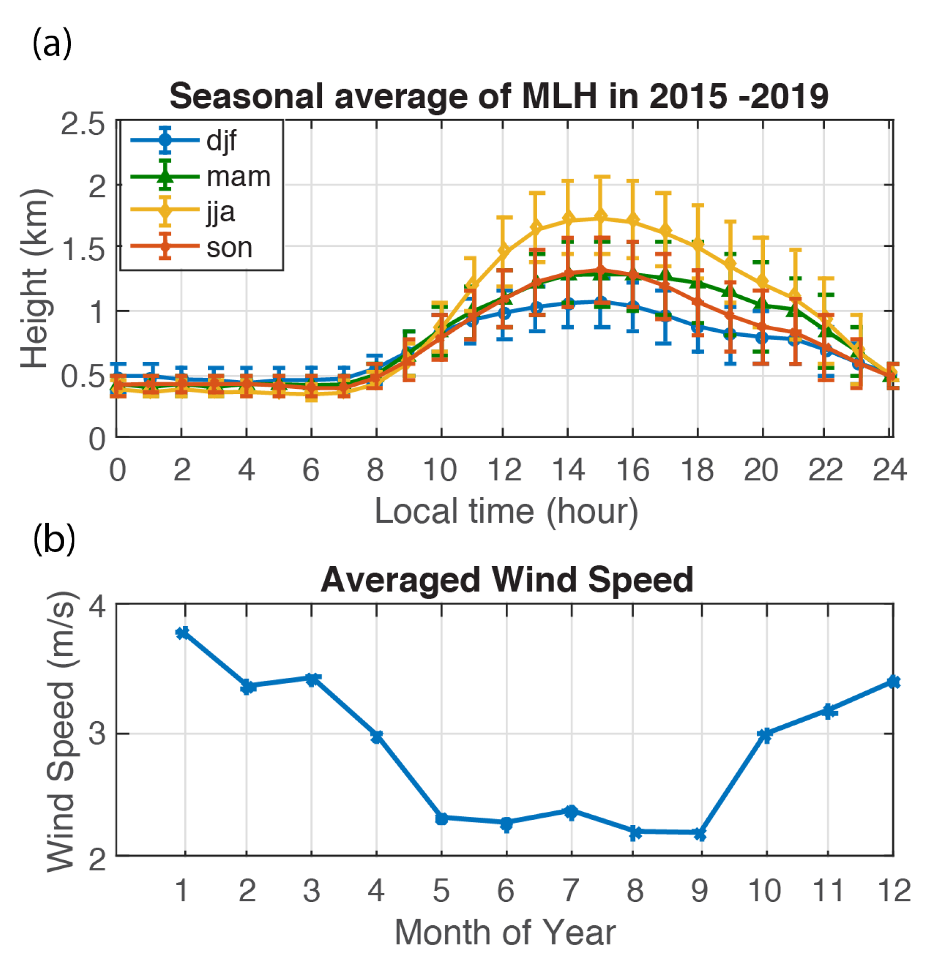
Figure 3a illustrates the seasonal and diurnal variations of the MLH from March 2015 to February 2019. From midnight (0:00, local time) until sunrise (7:00, local time), the MLHs remained stable (around 0.4 km) and did not show significant seasonal variation. During the morning transition (7:00–13:00), the MLH increased due to the enhanced thermal convection or entrainment and reached a maximum around 15:00 local time. Then MLH gradually decreased and remained above 0.7 km until 21:00, which was probably the result of an urban-heat-island effect. From 21:00 to 24:00, the MLH decreased rapidly to around 0.5 km. Comparing different seasons, during the convective period (around 15:00 local time), summer (June, July, August (jja)) had the highest MLH (1.76 ± 0.58 km, mean ± std), while winter (December, January, February (djf)) had the lowest MLH (=1.08 ± 0.38 km); the MLHs in spring and fall were about the same (MLH ≈ 1.3 ± 0.5 km). At 0:00–7:00, the averaged MLH was 0.37 km for summer, 0.45 km for winter, around 0.4 km in the spring and fall, which was opposite to the behavior for the convective period. This is reasonable because, when solar radiation is absent or still weak, the mechanical turbulence driven by the low jet wind may serve as the dominant mechanism for MLH development. Figure 3b shows the monthly averaged wind speed calculated from the data during 0:00–7:00 measured at the CCNY site. The wind speed was strongest in winter and generally weaker in summer, so that the MLH in winter exceeded the summer MLH in the night-time.

3.2. Correlation of Attenuated Backscatter Coefficients and Ground PM2.5

As mentioned in the introduction, in terms of air quality studies, ceilometers are capable of making 24 h continuous observations, but the detection performance is usually limited due to their relatively low SNR compared to the lidar system. To assess this, we investigated the correlation of ceilometer β a t t using a collocated lidar-retrieved aerosol backscatter coefficient + molecular backscatter coefficient ( β a + β m ). To exclude the influence of the lidar overlap function and CL51 background noise above MLH, backscatter coefficients between 700 m and the MLH (>700 m) were chosen for comparison. Table 2 shows the correlation of the CL51 and CHM15k ceilometers β a t t with the lidar retrievals on several days. Both ceilometers exhibited strong correlations with the lidar results, indicating that the ceilometers showed reasonable detection performance below the MLH and above the non-overlap range and that it is reasonable to study air quality profiles and structure using ceilometer β a t t within this range.
Next, we explored the vertical and temporal dependence of the correlation between the ceilometer β a t t and the ground-level PM2.5 concentration under clear and partly cloudy sky conditions in summer (July–August 2018) and winter (December 2018–February 2019). Since the Lufft CHM15k ceilometer was not available before 25 October 2018, here, we only study the correlation of PM2.5 with the β a t t from the Vaisala CL51 ceilometer. We used hourly PM2.5 measurements from the NYSDEC monitor station at CCNY, which was about 200 m away from the ceilometer location. To be temporally comparable with the PM2.5 concentrations, the ceilometer β a t t was averaged every hour. Additionally, in this analysis, to reduce the influence of the outliers, we removed the cloud contaminated β a t t based on the cloudbase height and applied robust regression to the ground PM2.5 concentration and β a t t using the MATLAB® Curve-fitting Toolbox™ to obtain the corresponding R 2 and regression slope [46]. The robust regression uses the bi-square weights method, and the weight of each data point depends on its distance from the fitted line, which minimizes the effect of outliers on the regression fit. It is worth noting that the reported R 2 here is a weighted R 2 , which is usually higher than the R 2 obtained by ordinary least square fit [47,48]. We used a linear model (y = ax + b) to fit the PM2.5 and β a t t .
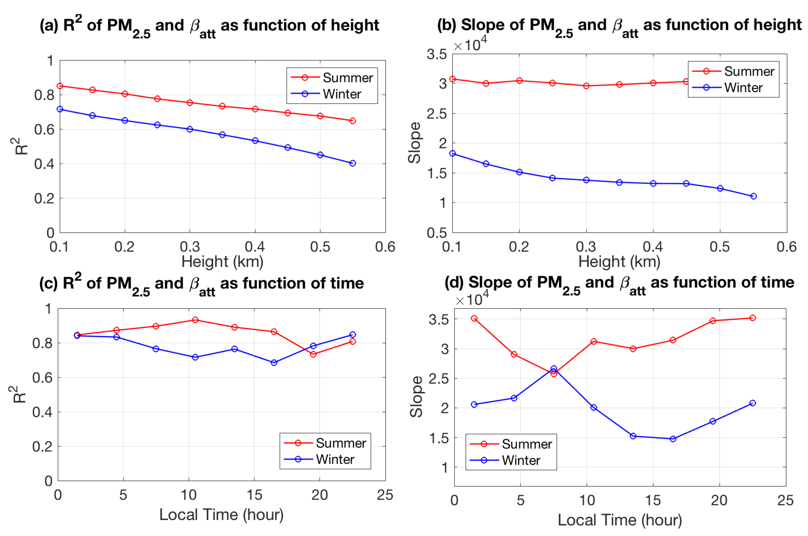
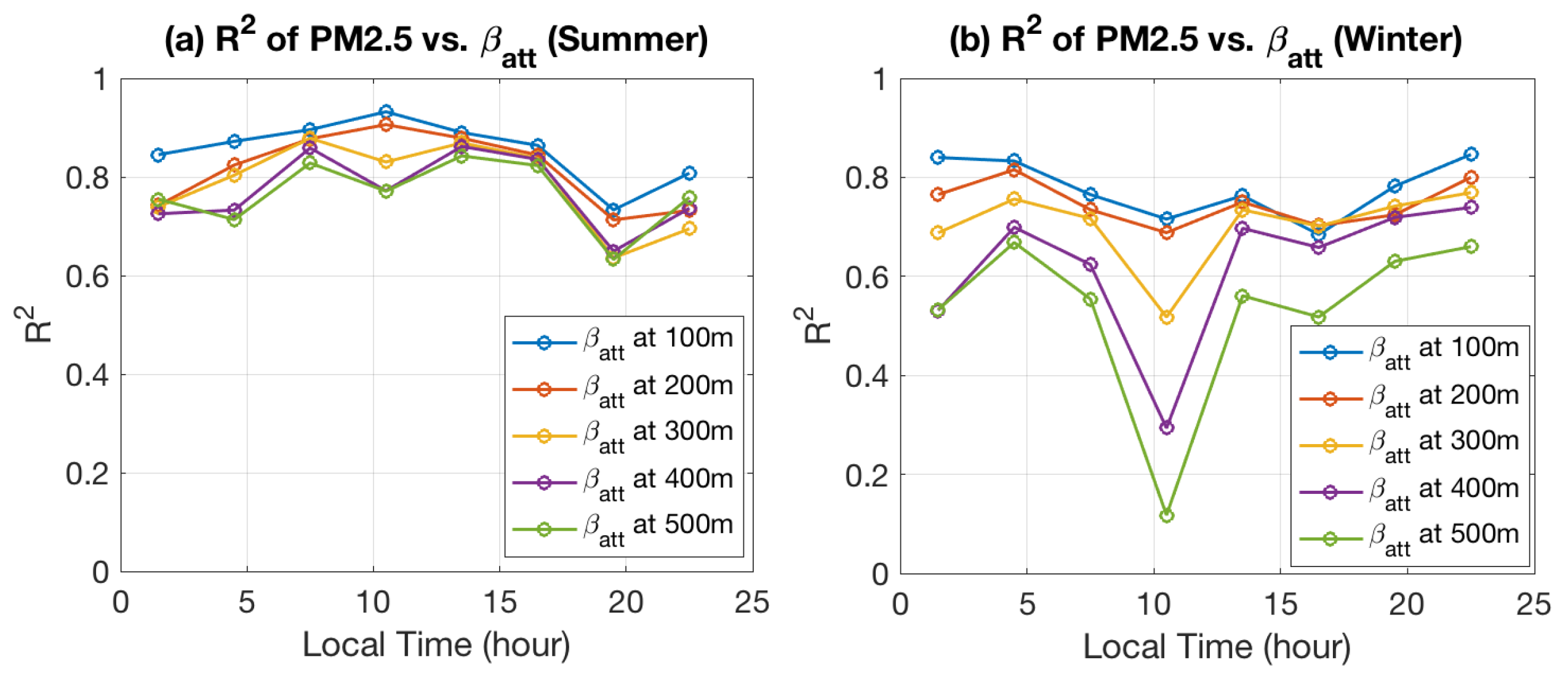
Figure 4a,b display the height dependence of the R 2 and the linear regression slope (a = P M 2.5 b β a t t , b is the intercept) in winter and summer, respectively. The regression slope a is approximately equal to P M 2.5 β a t t , when b is small. Generally, the R 2 decreases as the height increases. A strong correlation ( R 2 > 0.7) was found in the near-surface range (0.1–0.4 km) in summer. The correlation was better in summer than in winter, since the vertical mixing was stronger in summer than in winter due to stronger thermal turbulence, so that the β a t t better represents the surface PM2.5 level. On the other hand, the regression slope did not vary significantly with vertical height, but its value was almost twice as high in summer as in winter. This seasonal discrepancy in the slope may have been due to the net effect of different aerosol types, their size distribution and physical or chemical properties. Figure 4c,d show the time dependence of R 2 and the linear regression slope between the β a t t at 100 m and surface PM2.5. Each R 2 and slope was calculated from the corresponding β a t t at 100 m and surface PM2.5 within a 3 h time interval over all study days. The R 2 was relatively stable with respect to time, and the correlation in summer was slightly better than in winter at 5:00–19:00, which was due to the increasing convection or turbulent mixing. However, the slope in Figure 4d varied more significantly with respect to the time, implying the temporal variation of aerosol types or meteorological conditions. Figure 5 is similar to Figure 4c except that we observed the time dependence of R 2 at different heights in summer (Figure 5a) and winter (Figure 5b). In summer, as shown in Figure 5a, the R 2 decreased slightly as the height increased. During the convection period (12:00–18:00), R 2 remained nearly constant from 100 m to 500 m, which showed again that, in summer, the aerosol was more uniformly distributed over the vertical range. In winter, R 2 varied significantly with respect to the height, which implies that the aerosols were more stratified over the vertical altitude and decoupled from the surface.
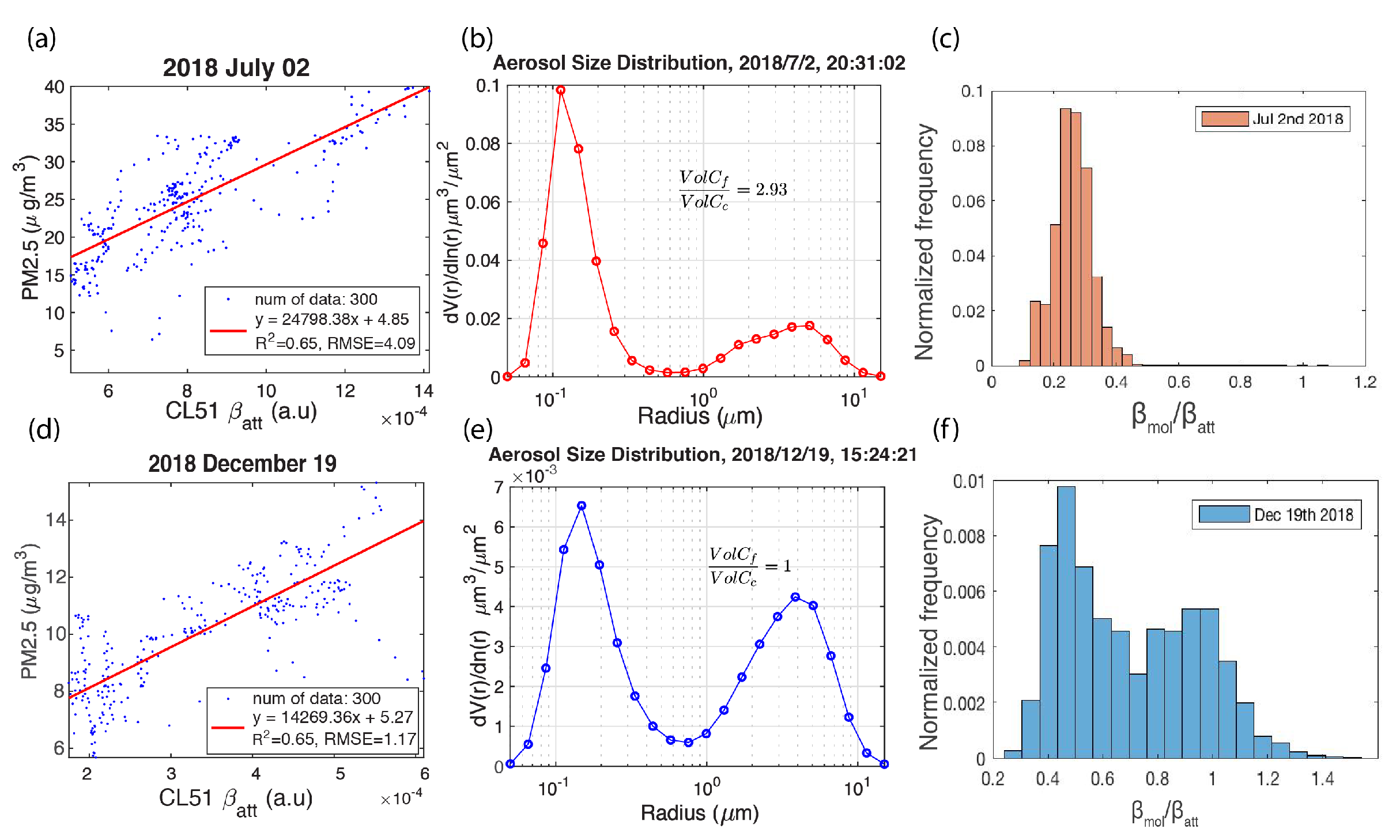
To further investigate the seasonal discrepancy of the slope and R 2 between PM2.5 and β a t t , two cases in summer and winter are presented in Figure 6. The correlation was evaluated between PM2.5 concentrations and β a t t with a temporal resolution of 10 min. The aerosol particle size distributions on 2 July 2018 and 19 December 2018 were obtained from aerosol inversion products at the AERONET CCNY site. Figure 6a illustrates the correlation of PM2.5 with β a t t on 2 July; the R 2 was 0.65 with RMSE = 4.8 and the slope = 2.5 × 10 4 . However, on December 19th (Figure 6d), the R 2 was 0.64 with RMSE = 1.19 and the slope = 1.4 × 10 4 . These results demonstrate a larger slope on 2 July than the slope on 19 December, which is consistent with the seasonal discrepancy highlighted in Figure 4b. The aerosol size distribution on 2 July 2018 (Figure 6b) indicates that, on this day, the aerosols were fine-modal dominated and the volume concentration ratio of fine mode to coarse mode was 2.93. On 19 December 2018 (Figure 6e), the volume concentration ratio of fine mode to coarse mode was one, indicating a greater coarse-mode aerosol contribution in the winter case than in the summer case. The PM2.5 mostly represents the mass of fine mode particle, whereas the ceilometer-measured β a t t are from particles of all sizes. Thus, fine-mode particles dominated the aerosols in summer resulting in a larger slope than that in winter (with more coarse-mode particles). Moreover, other effects may partially explain the observed discrepancy. For instance, the PM2.5 concentration and β a t t were generally smaller in the winter than in the summer, indicating that the aerosol loading is lower in the winter case. When the aerosol loading is low, the molecular contribution to the total β a t t becomes larger, leading to a smaller linear slope. To validate this, we evaluated the ratio of the molecular backscatter coefficient to the total attenuated backscatter coefficient. The molecular backscatter coefficients were calculated from radiosonde profiles measured at the Brookhaven National Laboratory site (Upton, New York, National Weather Service). Figure 6c,f display a histogram of the ratio of molecular to β a t t on 2 July and 19 December, respectively, demonstrating that the molecular backscatter contribution to the total attenuated backscatter coefficient was larger in the winter case than in the summer case, so the linear slope was smaller in winter than in summer. However, it should be noted that the molecular contribution did not affect the correlation coefficient between the surface PM2.5 and β a t t at each altitude. All of these effects can also ultimately alter the AOD-PM2.5 conversion slope.

3.3. Vertical Mixing of Aerosols in the ML

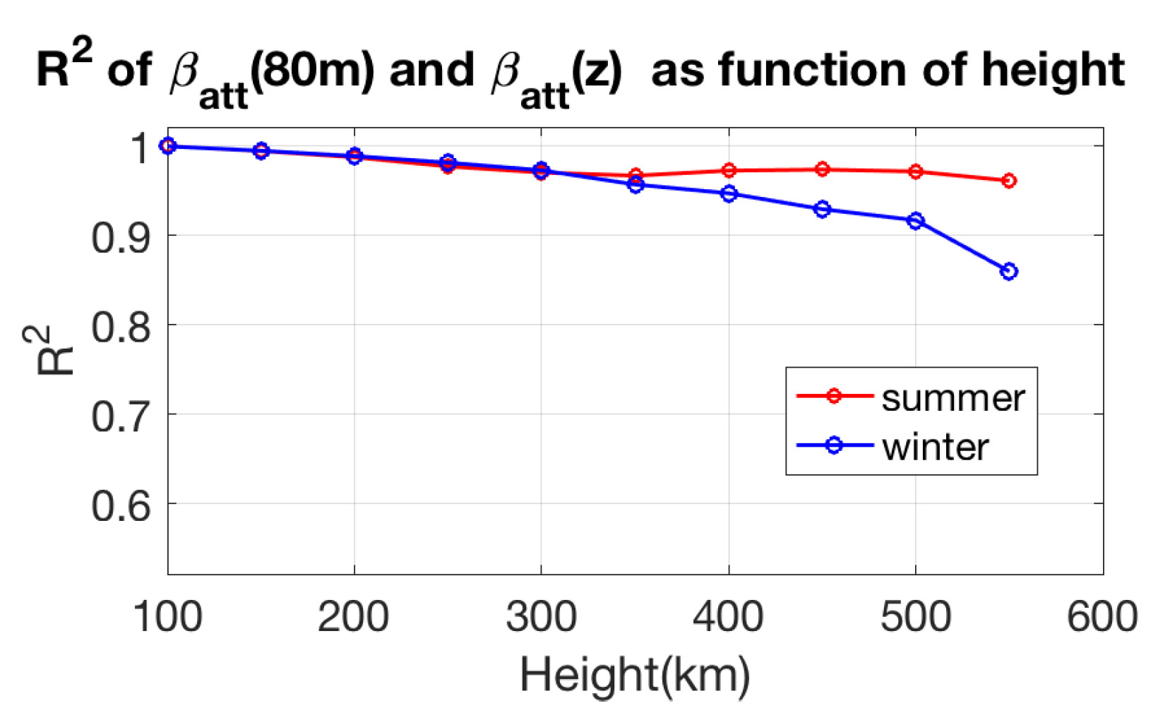
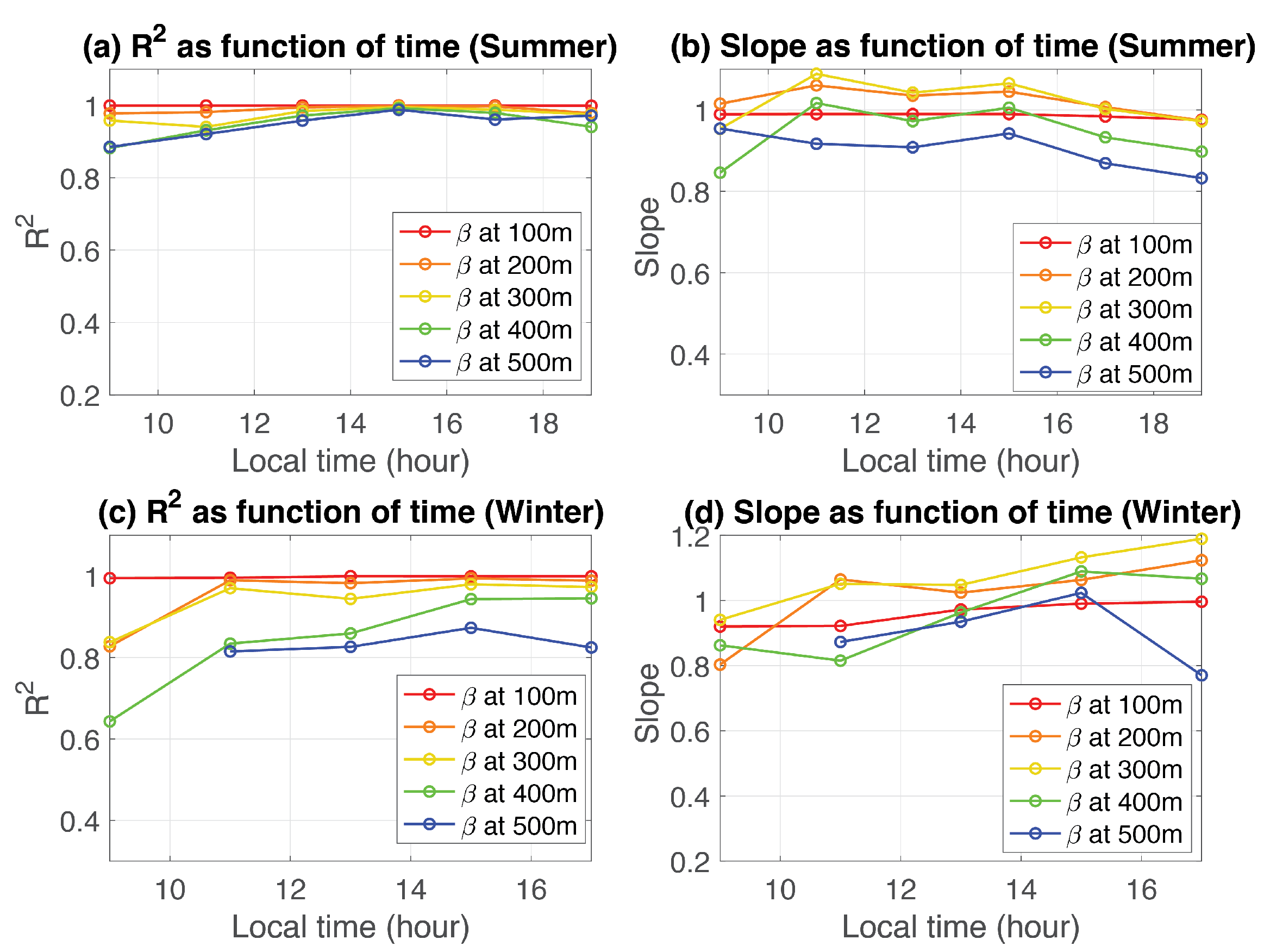
As mentioned previously, whether a columnar-averaged optical measurement (such as satellite AOD) can effectively estimate the near-surface PM2.5 depends on the aerosol vertical mixing level. To assess the vertical mixing of the aerosol within the lower part of ML, we investigated the linear correlation between the near-surface β a t t (at 80 m) with the β a t t at different heights (up to 500 m) within the ML, under clear sky conditions (no aerosol plumes or low clouds). In total there were 14 days’ data with six days in summer and eight days in winter. Within these 14 days, the two-way transmittance at 910 nm calculated from AERONET AOD were mostly above 0.9 ( Appendix A.2, Figure A1), indicating that the influence of the transmittance was relatively small. Figure 7 illustrates their correlation R 2 . For both summer and winter, the R 2 was greater than 0.95 up to 300 m. From 300 m to 550 m, the R 2 in summer remained around 0.95, while the R 2 in winter slightly decreased but was still above 0.85, showing that the aerosols were generally well-mixed within the ML up to 500 m for both seasons, with summer slightly better than the winter. Figure 8 shows the time variation in the correlation coefficient R 2 and the linear regression slope of near-surface β a t t (at 80 m) and the β a t t at different heights within the ML in summer (Figure 8a,b) and winter (Figure 8c,d) during the daytime. Note that, we only selected the β a t t ( z ) below the MLH for the regression; during the winter, the MLH in the morning can be below 500 m, so the R 2 and slope for β at 500 m in winter at 9:00 are not shown. The R 2 and regression slopes were relatively stable with respect to the time of day in summer. In summer, the R 2 at 400 m and 500 m slightly increased from 9:00 to 15:00, implying that the aerosol vertical mixing became stronger due to the solar radiation. The slope varied within 0.9–1.1 (Figure 8b). In winter, the R 2 below 400 m was generally high (greater than 0.8), while the R 2 above 400 m was moderate. At 9:00, the R 2 in winter at 400 m was relatively worse, at around 0.6. In sum, the aerosols were generally well-mixed within the lower part of ML up to 500 m and remained relatively stable during the daytime. The aerosol vertical mixing was slightly stronger in summer than in winter. Since the AOD-PM2.5 correlations depend on the aerosol vertical structure, the vertical correction of AOD by MLH (AOD/MLH) [11,12,17] can provide a better estimate of the surface aerosol concentration when the aerosols are well-mixed within the ML, as implied by the observation that the vertical correlation of the ceilometer backscatter did not degrade substantially.

4. Conclusions

Ceilometer-measured aerosol vertical profiles provide an opportunity to track MLH dynamics, aerosol vertical distribution, and even changes in aerosol composition. This information is of great value to validate weather and air quality models, to better understand air pollution episodes, and to improve the estimation of ground level PM2.5 concentrations from satellite AOD products.
Although the MLH from ceilometer measurement has been studied previously, each ceilometer model has some limitations and uncertainties due to the inherently weak SNR and complex aerosol structure in the lower troposphere. As demonstrated in this paper, applying a QC/QA process to the original ALH provided from the manufacturer’s software can improve the accuracy of the MLH results by removing outlier points. After the QC/QA process, the comparisons of MLH retrievals between lidar and the ceilometers demonstrated good consistency ( R 2 > 0.8, slope > 0.9). The seasonal and diurnal variations in MLH for 2015–2019 in the NYC were presented.
We also analyzed the seasonal and diurnal variations in the correlation between surface PM2.5 and the attenuated backscatter coefficient, as well as its vertical height dependence. We found that the R 2 values were generally high at the near-surface range and decreased with height. The R 2 in summer was better than in winter, which was due to better aerosol mixing within the ML in summer than in winter. In addition, the conversion coefficients of β a t t to PM2.5 and their regression slopes showed the seasonal discrepancy in summer and winter. In particular, the slope in summer was twice the value in winter, which can be partially attributed to differences in the aerosol size distribution, aerosol loading and type.
Lastly, we investigated the aerosol vertical mixing effect using the correlation between the ceilometer-attenuated backscatter at near-surface β a t t (80 m) and β a t t ( z ) at different heights within the ML. The results confirmed that the aerosols were generally well-mixed within the lower part of the ML during the daytime, even in a complex urban coastal environment with many local and regional emission sources. A broader investigation is ongoing to extend this work to higher altitudes in the ML under different diurnal and seasonal conditions.

Author Contributions

Conceptualization and methodology, D.L., Y.W., B.G. and F.M.; data curation, Y.W.; formal analysis, D.L. and Y.W.; resources, B.G. and F.M.; software, D.L. and Y.W.; supervision, F.M.; writing—original draft, D.L. and Y.W.; writing—review and editing, D.L., Y.W., B.G. and F.M. All authors have read and agreed to the published version of the manuscript.

Funding

This research was funded by the New York State Energy Research and Development Authority agreement No.137482.

Data Availability Statement

The data presented in this study are available on request from the corresponding author.

Acknowledgments

The authors would like to thank the New York State Department of Environment Conservation (NYSDEC), the NOAA and NASA for the surface PM2.5 concentration, radiosonde and AERONET data.

Conflicts of Interest

The authors declare no conflict of interest.

Abbreviations

The following abbreviations are used in this manuscript:
MLHMixing Layer Height
NYCNew York City
QA/QCQuality Control/Quality Assurance
MLMixing Layer
PM2.5Fine particulate matter with a diameter of less than or equal to 2.5 μ m
AODAerosol Optical Depth
GOES-CHEMChemical transport model from the Goddard Earth Observing System
CALIOPCloud-Aerosol Lidar with Orthogonal Polarization
CBLConvective Boundary Layer
PBLHPlanetary Boundary Layer Height
NASANational Aeronautics and Space Administration
NOAANational Atmospheric and Oceanic Administration
WCTWavelet Covariance Transform
SNRSignal-to-Noise Ratio
CCNYThe City College of New York
ALHAerosol Layer Height
AERONETAErosol RObotic NETwork
NYSDECNew York State Department of Environment Conservation
FOVField Of View
APDAvalanche Photodiode
PMTPhotomultiplier Tubes
BL-ViewVaisala Boundary Layer View software
CBHCloud Base Height
djfDecember, January, February
mamMarch, April, May
jjaJune, July, August
sonSeptember, October, November
RMSE               Root Mean Square Error
UTCCoordinated Universal Time
β a t t Attenuated Backscatter Coefficient
β a Aerosol Backscatter Coefficient
β m Molecular Backscatter Coefficient
ENEvening
NTNight
MTMorning Transition
CTConvection
ETEvening Transition

Appendix A

Appendix A.1. QA/QC Procedures

The principles of the QA/QC of MLH are described in the main text Section 3.1. Here, we describe the detailed QC/QA process as follows:
  • Step 1: Initialize the primary MLHs to be the lowest ALHs retrieved by ceilometers with a time resolution of 16 s for CL51 and 15 s for CHM15k, filling the missing value of MLHs with the null value.
  • Step 2: For each primary MLH, generate quality flag (mblfg) with initiate value 0.
  • Step 3: For each primary MLH, check the lowest CBH within 11 timestamps (about 3 min) sliding window, if any lowest CBH is less than 3 km, mark the current quality flag to be 1;
  • Step 4: Divide the MLHs into 5 intervals: evening (EN: from evening time to night time), night (NT: from night time to sunrise), morning transition (MT: from sunrise to noon), convection (CT: from noon to sunset) and evening transition (ET: from sunset to evening time). Set upper bound H ( t ) and lower bound threshold L ( t ) : ( H E N , L E N ), ( H N T , L N T ), ( H M T , L M T ), ( H C T , L C T ) and ( H E T , L E T ), where the subscripts indicate the certain time interval. Note that, during the morning transition, the upper bound threshold is a linear function of time. If the primary MLH exceeds the corresponding threshold, then mark the quality flag to be 1. Compare the MLHs during NT and MT with the noon MLH, if the MLH during NT and MT exceeds 100 m above noon MLH, mark quality flag to be 1. The thresholds are shown in Table A1.
  • Step 5: Set the MLHs with corresponding mblfg = 1 to be the null value and then check the continuity of the MLHs: For each MLH, apply running median (omit null value) with corresponding temporal sliding window ( Δ τ ); if the difference between the current MLH and the running median is greater than threshold ( Δ h ), then mark quality flag to be 1. This process is applied one or two times and values of and are chosen based on different time intervals. (Table A2).
  • Step 6: Set the MLHs with corresponding mblfg = 1 to a null value, and average all the MLHs every 10 min (omit null value).
Table A1. Thresholds of MLH used for QA/QC process step 4.
EveningNightMorning TransitionConvectionEvening Transition
SummerWinterSummerWinterSummerWinterSummerWinterSummerWinter
Time (UTC hour)0:00–2:000:00–2:002:00–12:002:00–14:0012:00–17:0014:00–17:0017:00–21:0017:00–21:0021:00–0:0021:00–0:00
H1 (km)1.450.650.7740.7250.21t–1.550.33t–3.832.21.952.451.4
L1 (km)0.10.10.080.080.10.10.20.20.10.1
Table A2. Sliding window length ( Δ τ ) and threshold ( Δ h ) used for QA/QC process step 5.
EveningNightSunrise-AfternoonAfternoon-Evening
SummerWinterSummerWinterSummerWinterSummerWinter
Time (UTC hour)0:00–2:000:00–2:002:00–12:002:00–14:0012:00–19:0014:00–17:0019:00–00:0017:00–00:00
Δ τ (hour)1st time0.50.50.50.50.170.170.50.5
2nd time\\110.50.50.50.5
Δ h (km)1st time0.10.10.10.10.10.10.150.15
2nd time\\0.10.10.150.150.30.3
The running median is applied one time during the evening, therefore only one set of sliding window and threshold are shown here.

Appendix A.2. Aerosol Optical Transmittance
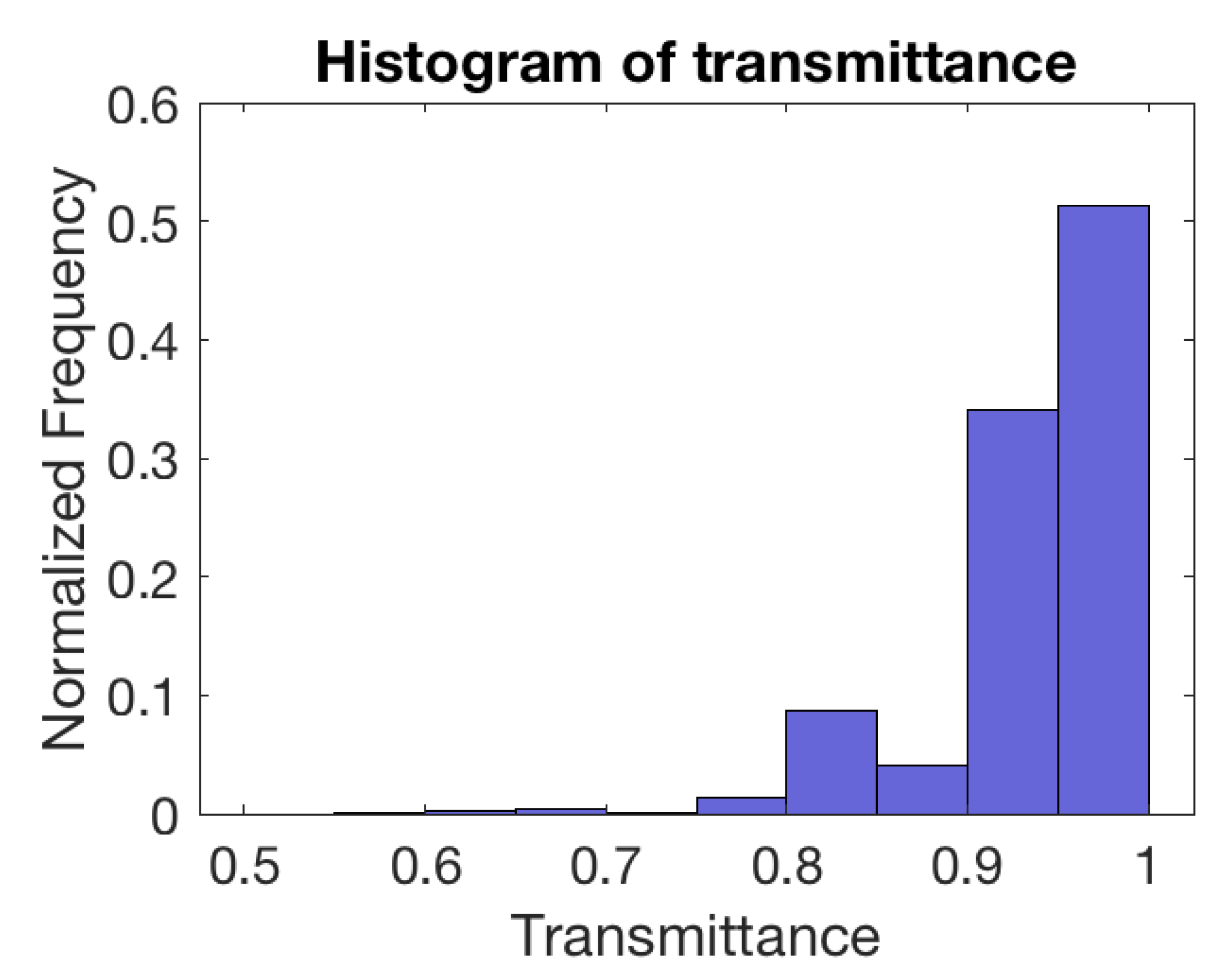
The aerosol transmittance at 910 nm is estimated using the AERONET level 1.5 AOD at 870 nm and the Angstrom exponent at 1020 nm and 870 nm for the study days, as shown in Figure 7 and Figure 8. Figure A1 shows a histogram of the two-way transmittance of all the available data in these 14 days.
Figure A1. Histogram of aerosol two-way transmittance at 910 nm calculated from AERONET AOD for the 14 studied days.
Remotesensing 14 06370 g0a1

References

  1. Xing, Y.F.; Xu, Y.H.; Shi, M.H.; Lian, Y.X. The impact of PM2.5 on the human respiratory system. J. Thorac. Dis. 2016, 8, E69. [Google Scholar] [PubMed]
  2. Du, Y.; Xu, X.; Chu, M.; Guo, Y.; Wang, J. Air particulate matter and cardiovascular disease: The epidemiological, biomedical and clinical evidence. J. Thorac. Dis. 2016, 8, E8. [Google Scholar] [PubMed]
  3. Kheirbek, I.; Wheeler, K.; Walters, S.; Pezeshki, G.; Kass, D.; Matte, T. Air pollution and the health of New Yorkers: The impact of fine particles and ozone. Environ. Prot. 2011, 3–4. [Google Scholar]
  4. Squizzato, S.; Masiol, M.; Rich, D.Q.; Hopke, P.K. A long-term source apportionment of PM2.5 in New York state during 2005–2016. Atmos. Environ. 2018, 192, 35–47. [Google Scholar] [CrossRef]
  5. Garratt, J.R. The atmospheric boundary layer. Earth-Sci. Rev. 1994, 37, 89–134. [Google Scholar] [CrossRef]
  6. Stull, R.B. An Introduction to Boundary Layer Meteorology; Springer Science & Business Media: Berlin, Germany, 2012; Volume 13. [Google Scholar]
  7. Miao, Y.; Liu, S.; Zheng, Y.; Wang, S. Modeling the feedback between aerosol and boundary layer processes: A case study in Beijing, China. Environ. Sci. Pollut. Res. Int. 2016, 23, 3342–3357. [Google Scholar] [CrossRef]
  8. Petaja, T.; Jarvi, L.; Kerminen, V.M.; Ding, A.J.; Sun, J.N.; Nie, W.; Kujansuu, J.; Virkkula, A.; Yang, X.Q.; Fu, C.B.; et al. Enhanced air pollution via aerosol-boundary layer feedback in China. Sci. Rep. 2016, 6, 18998. [Google Scholar] [CrossRef] [Green Version]
  9. Dong, Z.; Li, Z.; Yu, X.; Cribb, M.; Li, X.; Dai, J. Opposite long-term trends in aerosols between low and high altitudes: A testimony to the aerosol–PBL feedback. Atmos. Chem. Phys. 2017, 17, 7997–8009. [Google Scholar] [CrossRef] [Green Version]
  10. Mues, A.; Lauer, A.; Lupascu, A.; Rupakheti, M.; Kuik, F.; Lawrence, M.G. WRF and WRF-Chem v3.5.1 simulations of meteorology and black carbon concentrations in the Kathmandu Valley. Geosci. Model Dev. 2018, 11, 2067–2091. [Google Scholar] [CrossRef] [Green Version]
  11. Zhang, Y.; Li, Z. Remote sensing of atmospheric fine particulate matter (PM2.5) mass concentration near the ground from satellite observation. Remote Sens. Environ. 2015, 160, 252–262. [Google Scholar] [CrossRef]
  12. Yang, Q.; Yuan, Q.; Yue, L.; Li, T.; Shen, H.; Zhang, L. The relationships between PM2.5 and aerosol optical depth (AOD) in mainland China: About and behind the spatio-temporal variations. Environ. Pollut. 2019, 248, 526–535. [Google Scholar] [CrossRef] [PubMed]
  13. Liu, Y.; Park, R.J.; Jacob, D.J.; Li, Q.; Kilaru, V.; Sarnat, J.A. Mapping annual mean ground-level PM2.5concentrations using Multiangle Imaging Spectroradiometer aerosol optical thickness over the contiguous United States. J. Geophys. Res. Atmos. 2004, 109, D22. [Google Scholar] [CrossRef]
  14. Liu, Y.; Sarnat, J.A.; Kilaru, V.; Jacob, D.J.; Koutrakis, P. Estimating ground-level PM2.5 in the eastern United States using satellite remote sensing. Environ. Sci. Technol. 2005, 39, 3269–3278. [Google Scholar] [CrossRef] [PubMed] [Green Version]
  15. van Donkelaar, A.; Martin, R.V.; Park, R.J. Estimating ground-level PM2.5using aerosol optical depth determined from satellite remote sensing. J. Geophys. Res. 2006, 111, D21. [Google Scholar] [CrossRef]
  16. van Donkelaar, A.; Martin, R.V.; Spurr, R.J.D.; Drury, E.; Remer, L.A.; Levy, R.C.; Wang, J. Optimal estimation for global ground-level fine particulate matter concentrations. J. Geophys. Res. Atmos. 2013, 118, 5621–5636. [Google Scholar] [CrossRef] [Green Version]
  17. Zheng, C.; Zhao, C.; Zhu, Y.; Wang, Y.; Shi, X.; Wu, X.; Chen, T.; Wu, F.; Qiu, Y. Analysis of influential factors for the relationship between PM 2.5 and AOD in Beijing. Atmos. Chem. Phys. 2017, 17, 13473–13489. [Google Scholar] [CrossRef] [Green Version]
  18. Schafer, K.; Emeis, S.; Rauch, A.; Munkel, C.; Vogt, S. Determination of mixing layer heights from ceilometer data. Remote Sens. 2004, 5571, 248–259. [Google Scholar]
  19. de Haij, M.; Wauben, W.; Baltink, H.K. Determination of mixing layer height from ceilometer backscatter profiles. SPIE Remote Sens. 2006, 6362, 158–169. [Google Scholar]
  20. Eresmaa, N.; Karppinen, A.; Joffre, S.M.; Räsänen, J.; Talvitie, H. Mixing height determination by ceilometer. Atmos. Chem. Phys. 2006, 6, 1485–1493. [Google Scholar] [CrossRef] [Green Version]
  21. Münkel, C.; Eresmaa, N.; Räsänen, J.; Karppinen, A. Retrieval of mixing height and dust concentration with lidar ceilometer. Bound.-Layer Meteorol. 2006, 124, 117–128. [Google Scholar] [CrossRef]
  22. Gan, C.M.; Wu, Y.; Madhavan, B.L.; Gross, B.; Moshary, F. Application of active optical sensors to probe the vertical structure of the urban boundary layer and assess anomalies in air quality model PM2.5 forecasts. Atmos. Environ. 2011, 45, 6613–6621. [Google Scholar] [CrossRef]
  23. Hicks, M.; Demoz, B.; Vermeesch, K.; Atkinson, D. Intercomparison of Mixing Layer Heights from the National Weather Service Ceilometer Test Sites and Collocated Radiosondes. J. Atmos. Ocean. Technol. 2019, 36, 129–137. [Google Scholar] [CrossRef] [Green Version]
  24. Emeis, S.; Schäfer, K.; Münkel, C. Surface-based remote sensing of the mixing-layer height—A review. Meteorol. Z. 2008, 17, 621–630. [Google Scholar] [CrossRef]
  25. Menut, L.; Flamant, C.; Pelon, J.; Flamant, P.H. Urban boundary-layer height determination from lidar measurements over the Paris area. Appl. Opt. 1999, 38, 945. [Google Scholar] [CrossRef] [PubMed]
  26. Lammert, A.; Bösenberg, J. Determination of the convective boundary-layer height with laser remote sensing. Bound.-Layer Meteorol. 2005, 119, 159–170. [Google Scholar] [CrossRef]
  27. Cohn, S.A.; Angevine, W.M. Boundary Layer Height and Entrainment Zone Thickness Measured by Lidars and Wind-Profiling Radars. J. Appl. Meteorol. 2000, 39, 1233–1247. [Google Scholar] [CrossRef]
  28. Brooks, I.M. Finding Boundary Layer Top: Application of a Wavelet Covariance Transform to Lidar Backscatter Profiles. J. Atmos. Ocean. Technol. 2003, 20, 1092–1105. [Google Scholar] [CrossRef]
  29. Baars, H.; Ansmann, A.; Engelmann, R.; Althausen, D. Continuous monitoring of the boundary-layer top with lidar. Atmos. Chem. Phys. Discuss. 2008, 8, 10749–10790. [Google Scholar] [CrossRef] [Green Version]
  30. Steyn, D.G.; Baldi, M.; Hoff, R.M. The Detection of Mixed Layer Depth and Entrainment Zone Thickness from Lidar Backscatter Profiles. J. Atmos. Ocean. Technol. 1999, 16, 953–959. [Google Scholar] [CrossRef]
  31. Caicedo, V.; Rappenglück, B.; Lefer, B.; Morris, G.; Toledo, D.; Delgado, R. Comparison of aerosol lidar retrieval methods for boundary layer height detection using ceilometer aerosol backscatter data. Atmos. Meas. Tech. 2017, 10, 1609–1622. [Google Scholar] [CrossRef] [Green Version]
  32. Wagner, P.; Schäfer, K. Influence of mixing layer height on air pollutant concentrations in an urban street canyon. Urban Clim. 2017, 22, 64–79. [Google Scholar] [CrossRef]
  33. Heese, B.; Flentje, H.; Althausen, D.; Ansmann, A.; Frey, S. Ceilometer lidar comparison: Backscatter coefficient retrieval and signal-to-noise ratio determination. Atmos. Meas. Tech. 2010, 3, 1763–1770. [Google Scholar] [CrossRef] [Green Version]
  34. Wiegner, M.; Geiß, A. Aerosol profiling with the JenOptik ceilometer CHM15kx. Atmos. Meas. Tech. Discuss. 2012, 5, 3395–3430. [Google Scholar] [CrossRef]
  35. Wiegner, M.; Mattis, I.; Pattantyús-Ábrahám, M.; Bravo-Aranda, J.A.; Poltera, Y.; Haefele, A.; Hervo, M.; Görsdorf, U.; Leinweber, R.; Gasteiger, J.; et al. Aerosol backscatter profiles from ceilometers: Validation of water vapor correction in the framework of CeiLinEx2015. Atmos. Meas. Tech. 2019, 12, 471–490. [Google Scholar] [CrossRef] [Green Version]
  36. Madonna, F.; Rosoldi, M.; Lolli, S.; Amato, F.; Vande Hey, J.; Dhillon, R.; Zheng, Y.; Brettle, M.; Pappalardo, G. Intercomparison of aerosol measurements performed with multi-wavelength Raman lidars, automatic lidars and ceilometers in the framework of INTERACT-II campaign. Atmos. Meas. Tech. 2018, 11, 2459–2475. [Google Scholar] [CrossRef] [Green Version]
  37. Li, S.; Joseph, E.; Min, Q. Remote sensing of ground-level PM2.5 combining AOD and backscattering profile. Remote Sens. Environ. 2016, 183, 120–128. [Google Scholar] [CrossRef]
  38. Holben, B.N.; Eck, T.F.; Slutsker, I.; Tanre, D.; Buis, J.; Setzer, A.; Vermote, E.; Reagan, J.A.; Kaufman, Y.; Nakajima, T.; et al. AERONET—A federated instrument network and data archive for aerosol characterization. Remote Sens. Environ. 1998, 66, 1–16. [Google Scholar] [CrossRef]
  39. Dubovik, O.; King, M.D. A flexible inversion algorithm for retrieval of aerosol optical properties from Sun and sky radiance measurements. J. Geophys. Res. Atmos. 2000, 105, 20673–20696. [Google Scholar] [CrossRef] [Green Version]
  40. Wu, Y.; Chaw, S.; Gross, B.; Moshary, F.; Ahmed, S. Low and optically thin cloud measurements using a Raman-Mie lidar. Appl. Opt. 2009, 48, 1218. [Google Scholar] [CrossRef]
  41. Fernald, F.G.; Herman, B.M.; Reagan, J.A. Determination of Aerosol Height Distributions by Lidar. J. Appl. Meteorol. 1972, 11, 482–489. [Google Scholar] [CrossRef]
  42. Klett, J.D. Stable analytical inversion solution for processing lidar returns. Appl. Opt. 1981, 20, 211. [Google Scholar] [CrossRef] [PubMed] [Green Version]
  43. OTT HydroMet Fellbach GmbH. User Manual Lufft CHM15k Ceilometer. 2021. Available online: https://www.lufft.com/products/cloud-height-snow-depth-sensors-288/ceilometer-chm-15k-nimbus-2300/ (accessed on 25 November 2022).
  44. Hervo, M.; Poltera, Y.; Haefele, A. An empirical method to correct for temperature-dependent variations in the overlap function of CHM15k ceilometers. Atmos. Meas. Tech. 2016, 9, 2947–2959. [Google Scholar] [CrossRef] [Green Version]
  45. Vaisala Oyj. BL-View User Guide. 2018. Available online: https://docs.vaisala.com/r/M211185EN-E/en-US (accessed on 25 November 2022).
  46. The MathWorks, Inc. Curve Fitting Toolbox; MathWorks: Natick, MA, USA, 2018; Available online: https://www.mathworks.com/help/curvefit/least-squares-fitting.html (accessed on 25 November 2022).
  47. Holland, P.W.; Welsch, R.E. Robust regression using iteratively reweighted least-squares. Commun. Stat. Theory Methods 1977, 6, 813–827. [Google Scholar] [CrossRef]
  48. Willett, J.B.; Singer, J.D. Another cautionary note about R2: Its use in weighted least-squares regression analysis. Am. Stat. 1988, 42, 236–238. [Google Scholar]
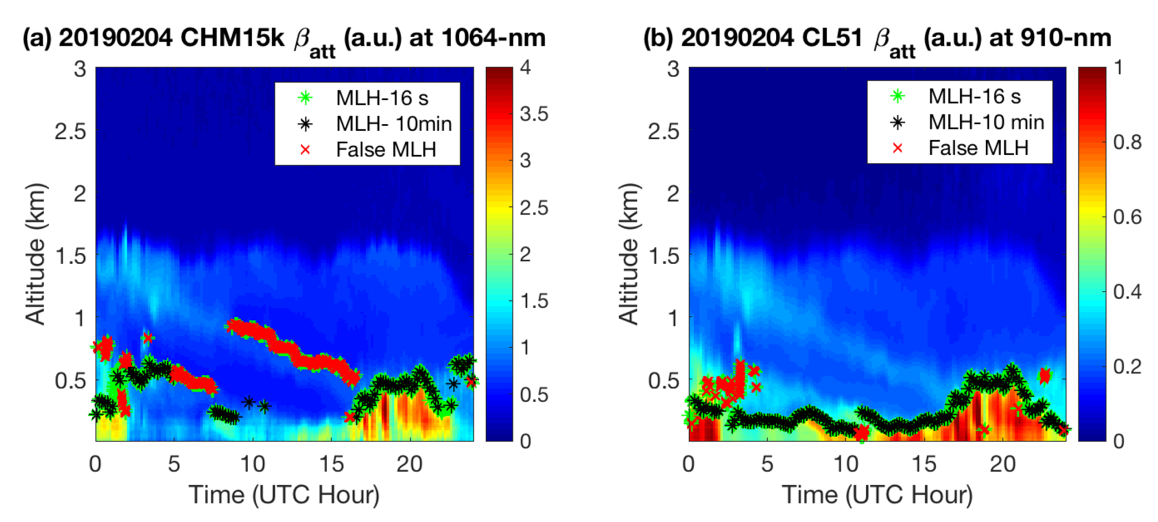
Figure 1. QC/QA process of original MLH detected by (a) CHM15k and (b) CL51 on 4 February 2019. The green symbols are the 16 s resolution lowest ALH detected by the ceilometers. The red cross symbols are the false MLH determined by the QC/QA process. The black symbols are the 10-minute resolution MLH results processed by QC/QA (Local time = UTC-5:00).
Remotesensing 14 06370 g001
Figure 2. (a) Scatterplot of MLHs retrieved from CL51 and CHM15k after QA/QC process. (b) Correlation R 2 between MLHs of CL51 and CHM15k as a function of time. (c) Correlation of MLHs retrieved from CL51 and CCNY-lidar. (d) Correlation of MLHs retrieved from CHM15k and CCNY-lidar.
Remotesensing 14 06370 g002
Figure 3. (a) Seasonal and diurnal hourly averaged MLHs retrieved from CL51 ceilometers from March 2015 to February 2019. Before 15 June 2018, MLHs were calculated using the WCT method under clear sky conditions. After 15 June 2018, the MLHs were calculated by the BL-view MLH determination algorithm combined with QC/QA process. The results are classified by the meteorological seasonal months of winter(December, January, February (djf), spring (March, April, May(mam)), summer (June, July, August(jja)) and fall (September, October, November(son)). (b) Monthly averaged wind speed from 0:00–7:00 local time measured at CCNY site from 2017–2019.
Remotesensing 14 06370 g003
Figure 4. Variation in the (a) regression correlation coefficient R 2 and (b) regression slope between ground PM2.5 concentration and β a t t of CL51 as a function of height. Variation in the regression correlation coefficient (c) R 2 and (d) regression slope of β a t t of CL51 at near-surface (100 m) with PM2.5 as a function of time.
Remotesensing 14 06370 g004
Figure 5. Variation in the regression correlation coefficient R 2 between ground PM2.5 concentration and β a t t of CL51 at different height as a function of time (a) in summer and (b) winter.
Remotesensing 14 06370 g005
Figure 6. Scatterplot of ground PM2.5 concentrations and CL51 β a t t on (a) 2 July 2018 and (d) 19 December 2018. Particle size distribution from AERONET on (b) 2 July 2018 and (e) 19 December 2018. Histogram of ratio of β m at 910 nm to CL51 β a t t on (c) 2 July 2018 and (f) 19 December 2018.
Remotesensing 14 06370 g006
Figure 7. Correlation coefficient R 2 of ceilometer near surface-attenuated backscatter β a t t (80 m) vs. β a t t ( z ) as a function of height.
Remotesensing 14 06370 g007
Figure 8. R 2 and slope of the correlation between β a t t (80 m) vs. β a t t ( z ) as a function of time (a,b) in summer and (c,d) winter, respectively.
Remotesensing 14 06370 g008
Table 1. Key specifications of CCNY-Lidar, Vaisala CL51 and Lufft CHM15k ceilometer [43].
InstrumentLaser SourceWave-Length (nm)Pulse Width (ns)Pulse EnergyBeam Divergence (mrad)Repetition Rate (Hz)Config-UrationReceiver FOV (mrad)Aprrox. Overlap Range (m)
CCNY-LidarNd:YAG1064 532 3558–12 1–2 < 1064 nm 2–3 < 1064 nm950 mJ 475 mJ 300 mJ<0.530coaxial2500 (∼95% overlap)
Vaisala CL51InGaAs Diode910 (±10)110 (50%)3 µJ (±20%)0.15 × 0.256.5 kcoaxial0.56230 (∼90% overlap) [36]
Lufft CHM15kmicro-chip Nd:YAG10641–57–9 µJ<0.35 k–7 kbiaxial0.451500 [33,44]
Table 2. Correlation of ceilometer-attenuated backscatter coefficient ( β a t t ) with lidar total backscatter coefficients ( β a + β m ) on different days.
Study DateCL51CHM15k *
R 2 RMSENum of Data R 2 RMSENum of Data
2018/07/090.895.57 × 10 5 4279N/AN/AN/A
2018/07/100.665.79 × 10 5 9010N/AN/AN/A
2018/10/250.851.98 × 10 5 30360.839.39 × 10 6 3658
2018/10/300.851.07 × 10 5 38460.791.46 × 10 5 3259
* The Lufft CHM15k ceilometer was installed in October 2018, so its data were not available on 9 July 2018 and 10 July 2018.
Publisher’s Note: MDPI stays neutral with regard to jurisdictional claims in published maps and institutional affiliations.