Article

UAV-Based Estimation of Grain Yield for Plant Breeding: Applied Strategies for Optimizing the Use of Sensors, Vegetation Indices, Growth Stages, and Machine Learning Algorithms

1
Hochschule Weihenstephan-Triesdorf, Markgrafenstrasse 16, 91746 Weidenbach, Germany
2
Saatzucht Josef Breun GmbH & Co. KG, Amselweg 1, 91074 Herzogenaurach, Germany
3
geo-konzept GmbH, Wittenfelder Strasse 28, 85111 Adelschlag, Germany
*
Author to whom correspondence should be addressed.
Remote Sens. 2022, 14(24), 6345; https://doi.org/10.3390/rs14246345
Submission received: 27 October 2022 / Revised: 6 December 2022 / Accepted: 10 December 2022 / Published: 15 December 2022
(This article belongs to the Section Remote Sensing in Agriculture and Vegetation)

Abstract

:
Non-destructive in-season grain yield (GY) prediction would strongly facilitate the selection process in plant breeding but remains challenging for phenologically and morphologically diverse germplasm, notably under high-yielding conditions. In recent years, the application of drones (UAV) for spectral sensing has been established, but data acquisition and data processing have to be further improved with respect to efficiency and reliability. Therefore, this study evaluates the selection of measurement dates, sensors, and spectral parameters, as well as machine learning algorithms. Multispectral and RGB data were collected during all major growth stages in winter wheat trials and tested for GY prediction using six machine-learning algorithms. Trials were conducted in 2020 and 2021 in two locations in the southeast and eastern areas of Germany. In most cases, the milk ripeness stage was the most reliable growth stage for GY prediction from individual measurement dates, but the maximum prediction accuracies differed substantially between drought-affected trials in 2020 (R2 = 0.81 and R2 = 0.68 in both locations, respectively), and the wetter, pathogen-affected conditions in 2021 (R2 = 0.30 and R2 = 0.29). The combination of data from multiple dates improved the prediction (maximum R2 = 0.85, 0.81, 0.61, and 0.44 in the four-year*location combinations, respectively). Among the spectral parameters under investigation, the best RGB-based indices achieved similar predictions as the best multispectral indices, while the differences between algorithms were comparably small. However, support vector machine, together with random forest and gradient boosting machine, performed better than partial least squares, ridge, and multiple linear regression. The results indicate useful GY predictions in sparser canopies, whereas further improvements are required in dense canopies with counteracting effects of pathogens. Efforts for multiple measurements were more rewarding than enhanced spectral information (multispectral versus RGB).

1. Introduction

Significantly raising crop yields and adapting plants to climate change while reducing environmental side effects is a crucial challenge to be addressed in plant breeding [1,2,3]. For wheat, which is one of the most important crops, plant breeding must therefore be intensified [2], making use of both genomic and phenomic methods [4]. Thus, precise, efficient, and objective plant phenotyping was identified as a major bottleneck [5,6].
Spectral sensors are promising for non-destructively providing valuable information about breeding traits in field environments by measuring canopy reflectance in indicative wavebands [7,8]. While hyperspectral sensing holds the highest potential for differentiating genotypes, a trade-off with respect to sensor costs, sensor handling, and the amount of generated data persists. Currently, multispectral sensing (MS) is recommended for traits such as grain yield and nitrogen uptake [9,10]. Still, simpler RGB cameras are useful for estimating senescence status, plant density, biomass, or plant height and provide higher pixel resolution [11,12,13]. Earlier approaches of field phenotyping applied ground-based vehicles [14]. However, recent technological advances and a decrease in costs favor the use of drones, i.e., unmanned aerial vehicles (UAVs) [11,15,16,17]. Notably, UAVs have the advantage of faster measurement without the risk of damaging trial plots. Moreover, UAVs have become more user-friendly, thus allowing the acquisition of spectral data with little effort. Still, the analysis of the data remains challenging [18,19].
With the increasing amount of UAV-based data generated, there is a growing demand for standardized workflows, which could also be used by practitioners in plant breeding without expert knowledge of the processing methods. Thus, reproducible, standardized [20], adaptable, accessible, and cost-efficient [21] methods are required.
Ultimately, GY is the most important trait in most cereal breeding programs, but it still relies on the destructive harvest of the plots, which is time-consuming and expensive. Thus, non-destructive in-season GY estimation could potentially replace conventional methods and would enable breeders to focus on germplasm with promising GY for the time-consuming visual evaluation of traits such as plant diseases, ear emergence, and other traits [5,22].
For wheat, a number of studies have shown the feasibility of in-season yield estimation using hand-held or vehicle-mounted sensors by means of vegetation indices [9,23,24,25]. However, the transfer to the specific conditions in breeding yards is often limited due to different trial conditions. This includes (i) the scale of farm-based versus breeding yard trials, (ii) the underlying variation in especially nitrogen fertilization for precision farming versus differing germplasm in phenotyping, (iii) the crop type of spring versus winter wheat, as well as (iv) the climatic conditions and the yield level.
For high-yielding but increasingly drought-affected mid-European conditions, the use of water band followed by red edge band indices acquired during milk ripeness was recommended [26]. Comparing UAV-based to ground-based sensing in a similar environment, Hu et al. [17] found a better association with GY from UAV data. Depending on plot type and vegetation index, either the flowering or dough ripeness stage was more suitable. For estimating above-ground biomass from MS and RGB UAV data, a study conducted in China reported the best correlations during heading, while the ranking of vegetation indices depended on the growth stage [27]. For GY prediction in spring barley under drought-affected German conditions, RGB and MS performed similarly, and predictions increased towards later growth stages and after rainfall [10]. However, data fusion from both sensors did not significantly improve the predictions in this study. Both early-stage vegetation cover and plant height were revealed to be significant predictors. Similarly, plant height and RGB indices were reported as indicators for GY and biomass in wheat [28,29].
With respect to machine learning algorithms, results are not consistent. The latter study [29] found better predictions using random forest (RF) than from stepwise multiple linear regression (MLR), support vector machine (SVM) regression, and extreme learning machine (ELM). Further studies confirmed the usefulness of RF in comparison to SVM for biomass estimation [30], to SVM and artificial neural networks (ANN) [31], and to SVM for UAV-based biomass estimation [29]. In contrast, differences between RF and SVM and deep learning were minor for soybean GY prediction [32]. Likewise, stepwise MLR performed better than RF for large-scale yield prediction [33]. For GY prediction in spring wheat, the Lasso regression was similar to SVM [34], and partial least squares regression (PLSR) was similar to linear regression [26].
Efficient phenotyping strategies using UAV should include the optimization of (i) the selection of suitable measurement dates, (ii) the choice of spectral sensors, their band configuration, and consequently, the available spectral parameters, and (iii) the use of machine learning algorithms. This study, therefore, aims at evaluating these factors for the in-season estimation of grain yield (GY) in real-world breeding yards by applying a custom-developed processing pipeline for the semi-automated analysis of UAV-based data.

2. Materials and Methods

2.1. Field Trials

Field trials were conducted by a plant breeder in two locations in the growing seasons of 2019/20 and 2020/21 (Figure 1a). The trials were located at varying sites in southeast Germany near Herzogenaurach (“HZ”; approximately 10.86E, 49.55N) and in eastern Germany near Morgenrot (“MR”; approximately 11.21E, 51.78N). The combinations of the two years and locations will be henceforth referred to as HZ_20, MR_20, HZ_21, and MR_21 for locations HZ and MR in the first and second year, respectively. Both locations are situated in the Köppen-Geiger climate zone Dfb (“Warm-summer humid continental climate”). Recent five-year average temperature and precipitation were 10.5 °C and 562 mm in HZ and 11.1 °C and 392 mm in MR. The MR trials were characterized by higher water-holding capacity with more homogenous soil (Tschernosem; [35]) and flat terrain. In contrast, soil texture was more heterogeneous (Stagnosol; [36]) on hilly terrain in HZ. Soil quality on a scale from 0 (lowest quality) to 100 (highest quality) according to the German soil inventory was 87, 90, 42, and 43–47 in MR_20, MR_21, HZ_20, and HZ_21, respectively.
Weather conditions were monitored using field weather stations at a distance of a few kilometers from the trials. In HZ, the first trial year was characterized by relatively dry and hot conditions during April and May, the months of main vegetative growth, whereas the second year was colder and more humid (Figure S1). In MR, precipitation was comparable in both years in April and May, whereas April temperature was lower in 2021 than in 2020. Within years, MR was mostly characterized by less precipitation than HZ, which, however, was compensated by higher soil water capacity.
The germplasm consisted of pre-selected material, F5 generation and older, as well as double haploid lines, without extreme genotypes in terms of morphology and phenology. The breeding program is targeted at the Central European market. In both years, both trials consisted of identical germplasm, which was grown without replication. To account for the heterogeneous soil, every fifth trial row was sown with one of two standard (‘references’) cultivars, ‘Bosporus’ and ‘Informer’.
The trials were predominantly sown in the second half of October and harvested in the last and first week of July and August, respectively. The plot size was 6 m2 in MR and 5.75 and 5.22 m2 in HZ_20 and HZ_21, respectively. Fertilization was conducted in compliance with local standards, and plots were kept weed-free. In contrast to MR, no fungicide was applied in the HZ trials.
Plots were harvested using a combine harvester to determine grain yield (GY) at kernel moisture of 14%. Prior to the harvest, the plots were visually screened, and a fraction of the plots was neglected for harvest based on pathogen scores, weak biomass growth, or plot damage due to lodging. Thus, GY was available from 4423 plots of the total 4930 plots in MR_20, from 4349 of 4923 plots in HZ_20, from 2787 plots of 3636 plots in MR_21, and from 2711 plots of 3588 plots in HZ_21. The slightly differing total number of plots in the two locations within years is due to additional plots with reference cultivars in MR. Preceding crops were rapeseed and sugar beet for the HZ trials and rapeseed for the MR trials, respectively.

2.2. UAV Imagery Acquisition and Preprocessing

Multispectral (MS) and RGB UAV-based data were acquired during all major growth stages throughout the growing season on 8, 10, 8, and 6 dates in the MR_20, HZ_20, MR_21, and HZ_21 trials, respectively (Table 1). Measurement intervals were narrower during the grain-filling phase to account for the senescence-related faster canopy differentiation during this phase (Figure S2).
In some trials, no MS data was captured on the first or last date due to the delay or advanced senescence, respectively. In MR_21 and HZ_21, plant height data from the Digital Elevation Model (DEM) was missing for 2 March 2021 and 25 March 2021, respectively, the dates when the reference DEM was acquired. Measurement days were characterized by mostly homogenous illumination conditions and wind speeds below 10 ms–1.
For RGB data, either a DJI P4-Pro (DJI, Shenzen, China) or a DJI P4-RTK with a built-in camera was used. Furthermore, a Sony Alpha 6000 (Tokyo, Japan) was attached to a DJI M6000 or an XR6 (AIR6 Systems GmbH, Klagenfurt am Wörthersee, Austria).
For MS data, a Tetracam µMCA was used in MR_20, HZ_20, and HZ_21, and a Tetracam MCAW (Tetracam Inc.; Chatsworth, CA, USA) in MR_21. The band-specific CMOS sensors have a resolution of 1.3 MP. The MS cameras were attached to a DJI M600 or an XR6. The MS cameras comprised six bands. For the MCA, a green and red band in the visible spectrum, two red edge bands, and two near-infrared bands (Table 2). For the MCAW, the second NIR band was replaced by another VIS band, which was, however, not included in the analysis. The full width at half maximum (FWHM) of the filters was 10 nm, except for the second NIR band of the MCA, for which the FWHM was 20 nm. Both types of MS cameras use an incident light sensor (ILS) with the same spectral sensitivity as used by the cameras for measuring concurrent illumination conditions. In MR_21, a defect of the ILS affected the multispectral data of the red band from April 28th on, so this band, as well as the M_NDVI and M_PSRI, were removed from the analysis for this trial.
The forward and sideward image overlap were targeted to be at a minimum of 80% and 75% at the HZ location and 80% and 60% at the MR location, respectively. Flight height was about 60–80 m for the MS cameras, 50 m for the RGB cameras in HZ_20, 25–35 m in HZ_21, and 55 m for the RGB cameras in MR_20 and MR_21. Flight speed was typically 4–8 ms–1 for the higher altitude flights for the MS camera and, depending on the flight height, 2–5 ms–1 for the flights for the RGB camera. The resulting pixel size of the orthomosaics was 3–6 cm for the MS data, 1–2 cm for the spectral RGB data, and 2–3 cm for the DEM data.
The raw data of the MS camera were preprocessed using the software PixelWrench2 or PixelWrench for Macaw (Tetracam Inc.; Chatsworth, CA, USA). To correct for the spatial offset, spatial co-registration was conducted for the individual bands. The data were calibrated based on the values of a grey reflectance standard of 22% reflectivity captured directly after take-off or prior to the landing of the UAV. Reflectance was calculated by dividing the up-welling radiation measured in each of the six bands by the down-welling radiation measured simultaneously by the corresponding band of the ILS.
The generated RGB and preprocessed MS images were processed using the software Agisoft Metashape Professional Edition (versions 1.5–1.8; Agisoft LLC., St. Petersburg, Russia). Processing comprised the image alignment for the generation of a sparse and dense point cloud, based on which the DEM and orthomosaics were generated. Ground control points (GCP) were taken in RTK-precision at nine positions distributed across each of the trials and highlighted by white markers in the field. Before generating the dense point cloud, the data were georeferenced to an accuracy of 2–3 cm by assigning the GCP coordinates to markers visible in the individual images.
Parcel boundary polygons were created using the software MiniGIS (versions 2.11–2.13; geo-konzept GmbH, Adelschlag, Germany) based on the GNSS-guided sowing of the trials.

2.3. Postprocessing of Spectral Data

Selected spectral parameters were considered in the data analysis (Table 2). For MS, four spectral vegetation indices were included together with the original bands, based on previous results recommending red edge indices [17,26] and the importance of senescence dynamics for GY as monitored by the PSRI index [37]. For the RGB data, the original bands were normalized by the sum of the digital numbers of all bands to account for changing illumination conditions. In addition to the individual bands, four RGB-based vegetation indices were included based on their previous recommendation for GY and GY-related traits [10,38,39,40,41,42]. In addition, plant height (R_PH) was calculated by subtracting the digital elevation model (DEM) at the beginning of vegetation growth (“reference model”) from the DEMs of the respective measurement date (“Di”), similarly as in [12]. Raster calculation was conducted on the pixel level to allow the extraction of quantiles using the input raster layer in a custom-made analysis pipeline developed in Python [43]. The raster data were extracted on the plot level using “Grid Statistics for Polygons” in SAGA [44]. In addition to the mean values, all quantiles were calculated in intervals of 5%, including minimum, median, and maximum, as well as the standard deviation. Prior to the extraction, plot boundaries were buffered inside by 20 cm, as in [10], in order to exclude the boundary pixels and to avoid errors due to possibly imprecise plot alignment. Subsequently, the data were stored in a custom-made PostgreSQL (PostgreSQL 12.12) database.
Table 2. Spectral parameters considered in this study. DN_: Digital Number, M_: Multispectral data, R_: RGB data, ρ: reflectance, Di: measurement date, Dr: reference data, 1 center wavelength.
Spectral ParameterEquationDescriptionReference
Multispectral (MS) Camera
M_G ρ G r e e n Green band, 530 nm 1
M_NDRE1 ρ N I R 1 ρ R E 1 ρ N I R 1 + ρ R E 1 Normalized difference red edge index 1[45]
M_NDRE2 ρ N I R 1 ρ R E 2 ρ N I R 1 + ρ R E 2 Normalized difference red edge index 2[45]
M_NDVI ρ N I R 1 ρ R e d ρ N I R 1 + ρ R e d Normalized difference vegetation index [46]
M_NIR1 ρ N I R 1 NIR band 1; 780 nm 1
M_NIR2 ρ N I R 2 NIR band 2; 900 nm 1
M_PSRI ρ R e d ρ G r e e n ρ N I R 1 Plant senescence reflectance index[47]
M_R ρ R e d Red band, 670 nm 1
M_RE1 ρ R E 1 Red edge band 1; 700 nm 1
M_RE2 ρ R E 2 Red edge band 2; 730 nm 1
RGB Camera
R_BN D N B l u e D N R e d + D N G r e e n + D N B l u e Normalized blue band
R_EVI2_green 2.5     R _ G N R _ R N R _ G N + 2.4     R _ R N + 1 Enhanced Vegetation
Index 2-Green
[39]
R_GLI 2     R _ G N R _ R N R _ B N 2     R _ G N + R _ R N + R _ B N Green leaf index[42]
R_GN D N G r e e n D N R e d + D N G r e e n + D N B l u e Normalized green band
R_PH D E M D i D E M D r Plant height derived from the digital surface model (DEM) at Day i (Di), corrected by the DEM at areference day (Dr)
R_RN D N R e d D N R e d + D N G r e e n + D N B l u e Normalized red band
R_TGI R _ G N 0.39     R _ R N 0.61     R _ B N Triangular greenness index[41]
R_VARI R _ G N R _ R N R _ G N + R _ R N R _ B N Visible Atmospherically
Resistant Index
[42]

2.4. Grain Yield Modeling

The data were analyzed in R [48]) using an automated processing pipeline based on the caret package [49]. Six machine learning algorithms (MLA) were chosen, including random forest (RF), gradient boosting machine (GBM), ridge regression (Ridge), partial least squares regression (PLSR), multiple linear regression (MLR), and support vector machine regression (SVM) based on the radial basis kernel. Using the spectral data with all statistical parameters (with respect to the extraction on the plot level), the data were split into 80% training data and 20% validation data [50] for each of the trials, using the same samples for each iteration within trials. As the GY data, all data were used as aggregated on the plot level. Input sensor data were centered and scaled to mean 0 and standard deviation 1. Automated outlier detection and filtering were applied to the predictor data based on local outlier factor [51] as identified from the Mahalanobis distance following principle component analysis using the R-package “bigutilsr” [52,53]. For training, initial standard settings of the caret package were used [49].
MLA parameters were tuned using 10-cross validation in the caret package [54]. The predictions on the test set data were compared to the measured yield using the coefficient of determination (R2) and the root mean square error (RMSE). Yield prediction in phenotyping requires sufficient relative discrimination of the data but can generally tolerate an offset in the prediction [22]. Thus, the comparison focuses on the R2 values, while RMSE values are provided in the Supplementary Material.
The processing pipeline allows the iteration over (i) different phenotypic plant traits, (ii) spectral parameters, (iii) the acquisition dates of the spectral parameters, (iv) statistical parameters concerning the extraction of the spectral data on the plot level, and (v) machine learning algorithms. For (ii), (iii), and (iv), combinations can be run optionally. Since the extraction of multiple statistical parameters on the plot level (iv) is the least costly among these settings, all of them were included per default. In addition to individual date models, multi-date models were tested, either using the complete seasonal data (“all times”) or by adding incrementally the data of the next measurement date (date increments 1 to i, with i being the number of measurement dates minus 2). Thus, for example, “date_increment_1” comprises the data of the first and second date (Figure S3). Modeling results were compared for the effect of MLA, measurement time, and spectral parameter with analysis of variance (ANOVA) followed by Tukey’s post hoc test calculated using the R-package “agricolae” [55].

3. Results

3.1. Descriptive Statistics

Substantial grain yield (GY) variation was observed between experimental plots within the four trials (Table 3). GY differed between trials, with the highest mean GY observed in MR_21 followed by GY observed in HZ_21, MR_20, and HZ_20, respectively. Thus, in both locations, GY was higher in 2021 than in 2020. Within both years, location MR achieved higher yields than location HZ. GY variation within trials was higher in 2020 (coefficient of variation, CV, of 16% and 15%) than in 2021 (CV of 10% and 9% in MR and HZ, respectively).
The spectral data measured through multiple growth stages describe growth curves, such as from the NDRE1 index for HZ_2020 (Figure S2). Index values of the NDRE1 increased approximately linearly during vegetative growth until the end of May, plateaued during flowering and milk ripeness, and decreased during ripening.

3.2. The Selection of Machine Learning Algorithms

The comparison of GY prediction results within trials showed distinct differences between (i) the suitability of growth stages, i.e., measurement time (“time”), generally followed by (ii) those between spectral parameters (SP), and (iii) different MLAs.
Comparing the prediction results (R2) across all SPs by analysis of variance (ANOVA) for the effects of time and MLA, a weak, though significant (p < 0.001) effect of the MLA selection was found in all trials except MR_21 (Table S3). In contrast, a dominant effect of measurement time was observed, whereas the MLA:time interaction was never significant.
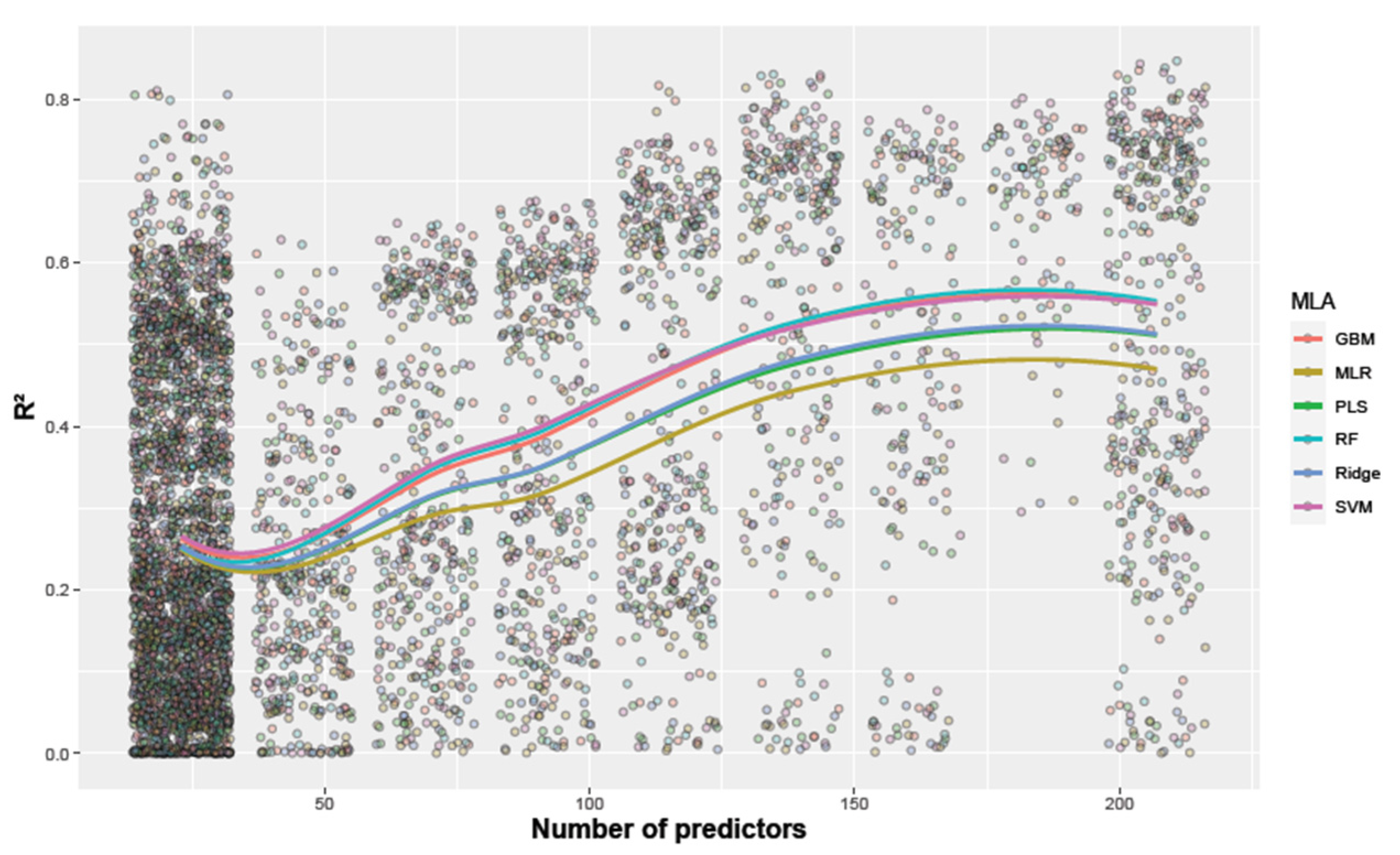
Compared by Tukey’s HSD post hoc test (Table 4), multiple linear regression (MLR) performed the weakest in all trials, though not significantly in MR_21 only. In contrast, either SVM or GBM ranked highest. In all trials, PLSR ranked maximum at fourth best, RF at positions 2 to 3, and Ridge regression at positions 2 to 4. The comparison of MLAs under consideration of the number of included predictors (Figure 2) showed little differences between MLAs for the individual date models with the fewest predictors (n = 23). However, increasing segregation becomes visible in multi-date models with more predictors, as visible from the smoothed curves. While MLR always showed the lowest R2 values, Ridge and PLS regressions performed similarly and ranked on ranks 4 and 5. SVM performed, in general, best for the models with fewer predictors. In comparison, RF was similar or tended to be slightly better for multi-date models. The performance of GBM was similar to that of SVM and RF.
Meanwhile, substantial differences were observed between MLAs in the time required for training (Figure S4). Irrespective of the number of predictors, MLR and PLS were by far the most time-efficient. For individual date models, SVM and RF required substantially more time than the other MLAs. While the required time steadily and steeply increased with more included predictors for RF and Ridge, the increase was less steep for GBM and especially SVM.

3.3. The Selection of Individual Measurement Dates

Significant effects of both the SP and time selection were found in all trials (Table S5), as well as a significant time: SP interaction.
Individual measurement dates showed weak (R2 < 0.30; MR_21 and HZ_21) to moderate (MR_20 and HZ_20) and, in general, improving predictions during vegetative growth stages until approximately mid-May (Figure 3 and Figure 4).Maximum pre-flowering R2 values observed from individual date models were 0.64 in MR_20 (05/19, R_VARI; Figure 4) and 0.52 in HZ_20 (05/20, R_RN), but only 0.17 in MR_21 (04/28, R_PH) and 0.29 in HZ_21 (05/14, R_EVI2_green).
In all trials except for HZ_20, R2 values increased to maximum values during early June (milk ripeness; Figure 4) with R2 = 0.81 in MR_20, R2 = 0.68 in HZ_20, and R2 = 0.31 in MR_21.

3.4. The Selection of Spectral Parameters

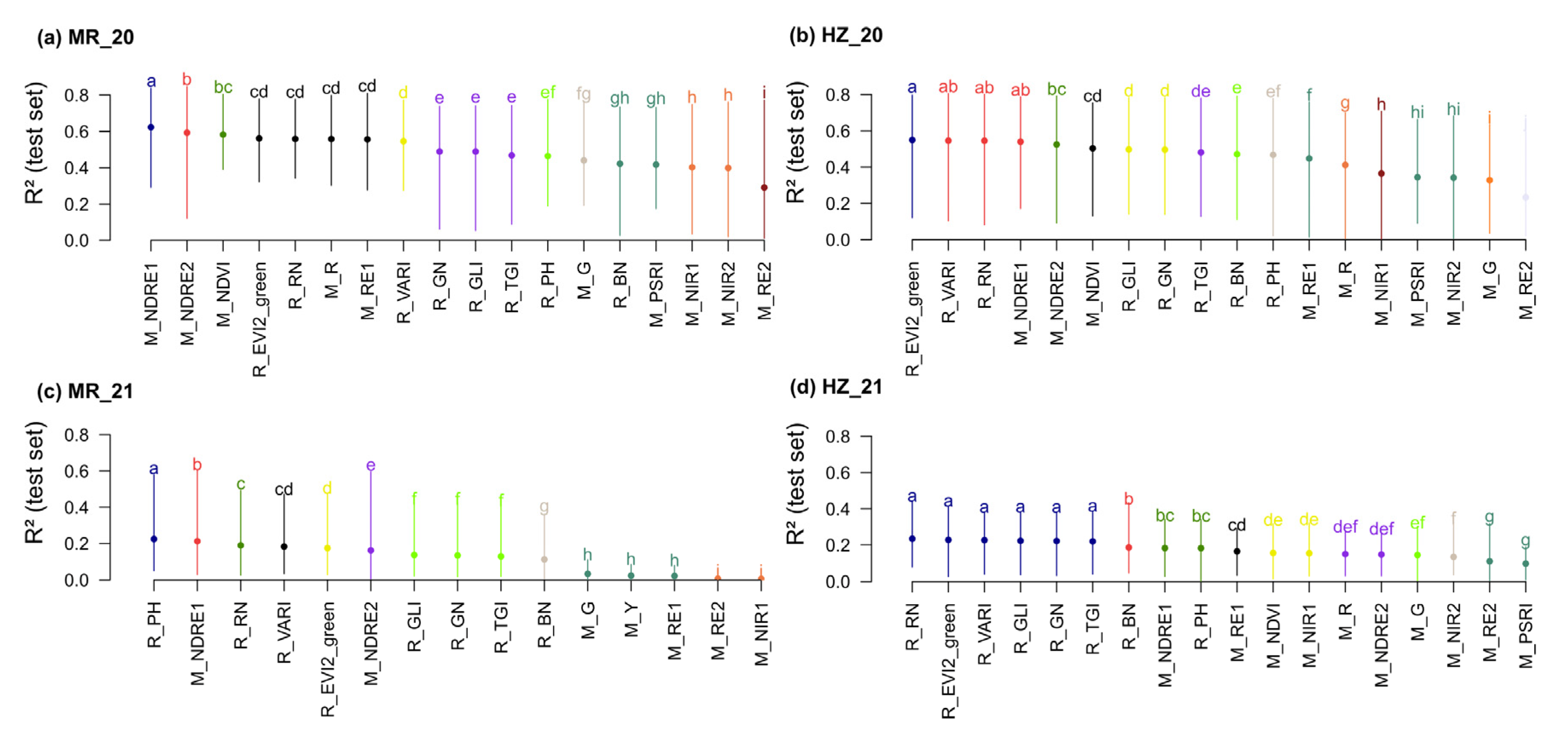
No significant MLA:SP interaction was found in any trial (Table S4). This suggests that SP can be compared irrespective of the MLA. In contrast, a dominant effect of the SP selection was observed. The overall ranking of SPs across all times and MLAs revealed the highest R2 values from the M_NDRE1 index in MR_20, closely followed by the M_NDRE2 and the M_NDVI (Figure 5). In contrast, in HZ_20, on average best prediction results were found from three RGB-based spectral parameters, followed by the group of multispectral indexes M_NDRE1, M_NDRE2, and M_NDVI.
In 2021, the prediction results were distinctively weaker. In MR_21, plant height (R_PH) ranked highest together with M_NDRE1, followed by the three RGB-based spectral parameters. The latter ranked highest in HZ_20 and HZ_21 (R_ N, R_VARI, and R_EVI_green). HZ_21 was characterized by the markedly weak performance of all multispectral spectral parameters, which all lagged behind all tested RGB-based SPs.

3.5. The Use of Incremental Date Combinations

The incremental combination of spectral data from multiple growth stages generally improved the predictions in comparison to the individual results of the included dates (Figure 3). R2 values in multi-date models steadily increased towards the full model, which included data from “all dates”. However, with generally higher prediction levels in MR_20 (Figure 3a) and HZ_20 (Figure 3b), a saturation was observed. Thus, improvements between date_increment_5 and the full model (MR_20; Figure 3a) and between date_increment_5, date_increment_6, date_increment_7, and the full model (HZ_20; Figure 3b) were only marginal and often not significant when compared for each SP (Table S1).
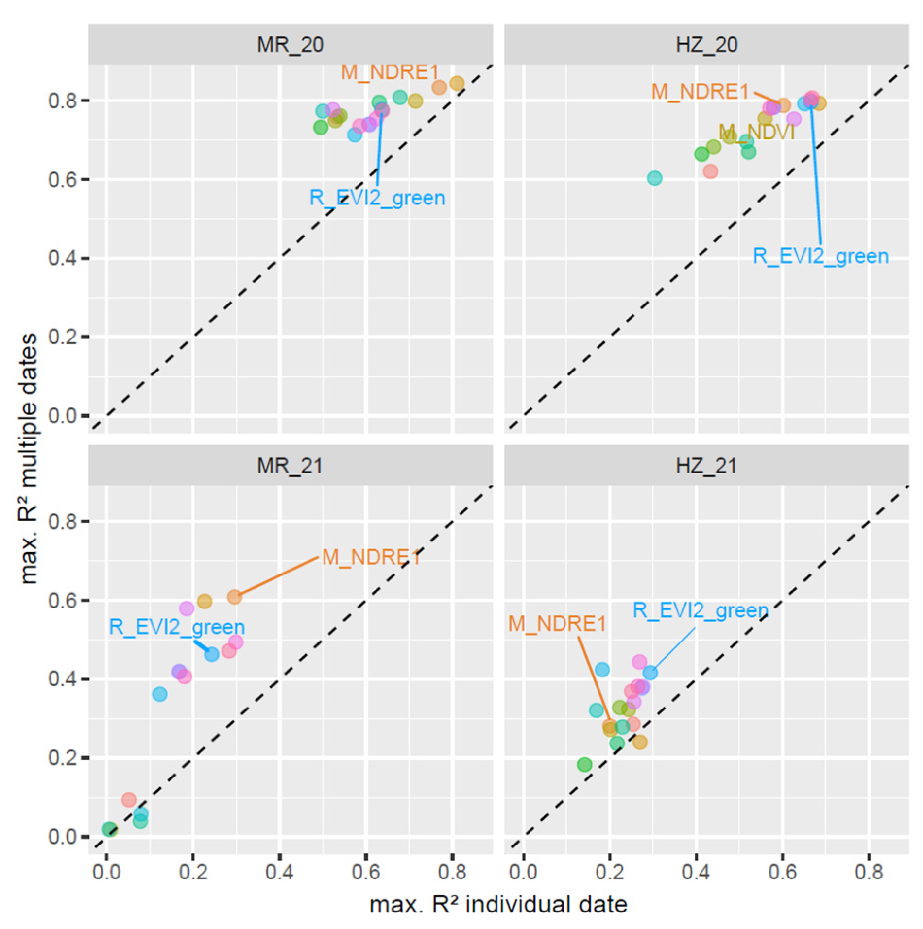
In general, the ranking of SPs from individual date models was correlated with the ranking from multi-date models (Figure 6). In HZ_20 and especially MR_20, SPs with weaker performance in individual date models profited more from the multi-date approach than SPs with high R2 values on individual dates. Therefore, maximum R2 values from multi-date models were similar from all SPs (Figure 6). In contrast to 2020 and to the best individual date SPs, in MR_21 and HZ_2, SPs with poor performance from individual date models hardly improved in the multiple-date approach (Figure 6).

4. Discussion

Based on the evaluated options for improving UAV-based GY estimation, this study suggests that the selection of suitable growth stages for spectral measurement is crucial but should be complemented by the proper selection of spectral parameters. In contrast, the selection of common machine learning algorithms had a comparably smaller effect.

4.1. The Influence of Growth Stage and Trial Conditions

The GY of small grain cereals is formed over time and through a complex interaction between the three yield components of ear density, the number of kernels per ear, and kernel weight [56,57]. However, non-imaging methods are not able to reliably measure any of these components on the canopy level. Still, the detection of plant traits correlated with GY explains that reasonable predictions can be observed. These traits include early vigor [58], biomass, chlorophyll content, and senescence status [59]. The results suggest that the flowering and milk ripeness stages are the most suited for GY prediction—the stages until which the vegetative development in biomass and plant height is completed. The suitability of these growth stages is in line with multiple previous studies on winter wheat [25,26,60] and spring wheat [61,62]. In contrast, continuously increasing predictions were observed in a study of spring barley [10].
While GY formation continues after milk ripeness, sufficient canopy greenness appears to be necessary for collecting meaningful data. Stay-green characteristics, as measured during later growth stages, can be beneficial for GY [63]. However, genotypic differences in flowering date and subsequently shifted development were not closely correlated with GY in the present data (not shown) but increasingly influenced the variation in the spectral data during the senescence phase [64].
The two study years were characterized by contrasting weather conditions with pronounced drought and heat in both MR_20 and HZ_20 in comparison to moderate temperatures in MR_21 and HZ_21 (Figure S1). Consequently, vegetative growth was stronger in 2021 than in 2020. Moreover, yield formation in 2021 was influenced by fungal diseases, which were neglectable in the first year. While spectral prediction requires the ranking in spectral data during measurement to be correlated with the later GY ranking, the differing disease susceptibility appears to counteract the correlation over time [62]. These findings are in line with two previous studies in a similar environment, where GY prediction in a dry year was more accurate than in a moist year [9,26].

4.2. The Advantage of Multi-Temporal Data

While many individual date models did not achieve satisfactory predictions, multi-date models showed the potential to (i) improve the predictions (Figure S3) and (ii) compensate for omitting one of the best individual dates. Thus, in practice, it will be difficult to measure on the best individual dates, both for practical reasons and due to non-predictable phenological shifts between years. In addition, the recommended milk ripeness stage (Section 4.1) is not yet reliably confirmed for differing trial conditions. Instead, using data from multiple dates appears to be a robust strategy for exploiting the prediction potential. The robust, but not eminently better, predictions in 2020 confirm the results of previous multi-date approaches [65,66,67]. In contrast, the advantage of multi-date models was more evident in 2021, with poor individual date models. This suggests that predictions were only possible through incorporating traits with influence on GY over time. GY prediction was likely possible through detecting biomass variation in 2020—the dominant trait under low-pathogen conditions [26]. In contrast, pathogen-triggered differences in senescence may have required multi-date models in 2021.

4.3. The Comparison of Machine Learning Algorithms

The present results suggest the use of SVM, while GBM and RF achieved almost similar results, however. The smaller differences compared to those reported in some previous studies may be related to the relatively large dataset and the high number of predictors included. In contrast, RF was superior over SVM for biomass prediction in wheat [30,68] and over SVM for UAV-based biomass estimation [29]. However, as in the present study, few differences were reported for soybean GY prediction between RF, SVM, and a deep learning approach [32]. While MLR could compete with other algorithms in the individual date models, it likely suffered from overfitting when more predictors were included. This is in line with the good performance of the MLR in comparison to RF in models with fewer predictors [33].
When also considering training time, the results suggest that RF and ridge regression should be avoided for larger datasets. These findings are only partly in line with previous results, where training time for RF was about ¼ to 3 that required for SVM [68]. Likewise, the better and worse processing performance of RF and SVM was reported compared to GBM, respectively, for classification applications [69]. Differences are likely related to the differing number of features and samples in the present study. For ridge regression and SVM, results are in line with [34], who reported much better computational efficiency of Lasso, which is similar to ridge regression, in comparison to SVM for a low number of predictors.
To sum up, differences between MLAs are likely related to the used data type (UAV vs. ground-based vs. satellite-based), the number and type of features (here many related statistical parameters on the plot level), the variation related to soil differences and genotypic variation versus nitrogen fertilization, and are therefore not straightforward to transfer.

4.4. The Selection of Sensors and Spectral Parameters

From the multispectral data, both vegetation indices, including red edge information, were confirmed to be more reliable than the ‘standard’ vegetation index NDVI. This phenomenon is frequently associated with higher sensitivity of the red edge spectrum compared to the red band as well as its relationship with chlorophyll content, which influences photosynthesis and, thus, GY [9,70]. However, the M_NDRE1 and M_NDRE2, differing in the position of the red edge band at 700 nm and 730 nm, generally achieved similar results. This is in line with the mostly homogenous performance of 22 indices, including red edge bands [26]. In contrast, the PSRI, with its expected sensitivity for senescence status, never showed a notable advantage over the NDVI and red edge indices. The original bands of the multispectral camera were included in the analysis for comparison with the bands of the RGB camera. Unlike the latter, their poor performance confirms the need to use vegetation indices or to combine multiple bands instead [33]. Further improvements may be expected from the use of other spectral bands, notably in the water absorption feature around 970 nm [26,61,71].
The surprisingly similar predictions from RGB-based indices, but also the RGB-red band (R_RN), as from the multispectral indices, indicate that not only the direct detection of above-ground biomass was indicative for GY prediction since the NIR bands of the multispectral camera should have shown an advantage for biomass. Instead, the exceptionally drought-influenced sparse canopies in 2020 are likely to have favored the RGB camera. Thus, through its higher ground-pixel resolution, the RGB camera may have captured variation in canopy cover, which in turn can be better correlated to biomass than spectral indices [58]. The suitability of RGB data is in line with similar results for ground cover estimation from an RGB as from a color infrared camera [13], good correlations from RGB-based indices with biomass [29], and similar [10] or better [71] results for GY prediction from RGB than from multispectral data.

5. Conclusions

This study on spectral UAV-based GY prediction does not aim to exhaustively evaluate each of the studied factors but to evaluate potentials and limitations and the interaction of these factors. It concludes to prioritize (i) the selection of suitable growth stages followed by that of (ii) spectral parameters, whereas similar predictions can be achieved from (iii) RGB and multispectral cameras and from (iv) various machine learning algorithms.
With respect to (i), generally, the milk ripeness stage was the most useful. Among spectral parameters, similar predictions were observed from the best RGB indices as from the multispectral red edge indices. Combining data from multiple dates holds the potential for improving predictions. Considering the different prediction accuracies from maximum R2 = 0.81–0.85 in the drought-affected trials in 2020 compared to R2 = 0.44 and 0.61 under wetter, pathogen-affected conditions, trial and weather-specific limitations need to be further addressed. Follow-up research should include the assessment of (i) feature selection with respect to the statistical parameters on the plot level and measurement dates, (ii) the plot boundary edge effect, (iii) efficient strategies for the selection and reduction of the number of training data, and (iv) further approaches for the fusion of sensors, spectral parameters, and measurement dates.

Supplementary Materials

The following supporting information can be downloaded at: https://www.mdpi.com/article/10.3390/rs14246345/s1. Table S1: Comparison of R2 results by time (YYYY-MM-DD) and spectral parameter. Table S2: Comparison of RMSE results [kg plot−1] by time (YYYY-MM-DD) and spectral parameter. Table S3: Results of analysis of variance for comparing the R2 values of GY prediction for the effect of machine learning algorithm (MLA) and measurement time. Table S4: Results of analysis of variance for comparing the R2 values of GY prediction for the effect of machine learning algorithm (MLA) and spectral sensor value (SP). Table S5: Results of analysis of variance for comparing the R2 values of GY prediction for the effect of measurement time and spectral sensor value (SP). Figure S1: Weather conditions in the four location*trial combinations. Figure S2: Seasonal development of the mean values of the multispectral NDRE1 index. Figure S3: Difference between the R2 values from M_NDRE1 multi-date models and the models of the individual dates contributing to the multi-date models. Figure S4: Effect of number of predictors on the time for training by machine learning algorithm at the example of MR_20.

Author Contributions

Conceptualization, L.P., A.H., L.R., J.S.-S. and P.O.N.; Data curation, L.P.; Formal analysis, L.P. and J.S.-S.; Funding acquisition, A.H. and P.O.N.; Investigation, L.R. and J.S.-S.; Methodology, L.P. and P.O.N.; Project administration, A.H. and P.O.N.; Resources, A.H., L.R., J.S.-S. and P.O.N.; Supervision, A.H. and P.O.N.; Visualization, L.P.; Writing—original draft, L.P.; Writing—review and editing, J.S.-S. and P.O.N. All authors have read and agreed to the published version of the manuscript.

Funding

This research was supported by funds of the Federal Ministry of Food and Agriculture (BMEL) based on a decision of the Parliament of the Federal Republic of Germany via the Federal Office for Agriculture and Food (BLE) under the innovation support program for the project 2818407A18.

Data Availability Statement

Data are available from the authors upon reasonable request.

Acknowledgments

The authors are grateful to the BMEL for the funding of the project. The authors gratefully acknowledge the administrative support by the Institute for Biomass Research of the HSWT and technical support by the Competence Centre for Digital Agriculture of the HSWT.

Conflicts of Interest

The authors declare no conflict of interest.

References

  1. Lobell, D.B.; Schlenker, W.; Costa-Roberts, J. Climate Trends and Global Crop Production Since 1980. Science 2011, 333, 616–620. [Google Scholar] [CrossRef] [PubMed] [Green Version]
  2. Ray, D.K.; Mueller, N.D.; West, P.C.; Foley, J.A. Yield Trends Are Insufficient to Double Global Crop Production by 2050. PLoS ONE 2013, 8, e66428. [Google Scholar] [CrossRef] [PubMed] [Green Version]
  3. Tilman, D.; Balzer, C.; Hill, J.; Befort, B.L. Global Food Demand and the Sustainable Intensification of Agriculture. Proc. Natl. Acad. Sci. USA 2011, 108, 20260–20264. [Google Scholar] [CrossRef] [PubMed] [Green Version]
  4. Marsh, J.I.; Hu, H.; Gill, M.; Batley, J.; Edwards, D. Crop Breeding for a Changing Climate: Integrating Phenomics and Genomics with Bioinformatics Crop Breeding for a Changing Climate: Integrating Phenomics and Genomics with Bioinformatics. Theor. Appl. Genet. 2021, 134, 1677–1690. [Google Scholar] [CrossRef] [PubMed]
  5. Araus, J.L.; Cairns, J.E. Field High-Throughput Phenotyping: The New Crop Breeding Frontier. Trends Plant Sci. 2014, 19, 52–61. [Google Scholar] [CrossRef]
  6. Houle, D.; Govindaraju, D.R.; Omholt, S. Phenomics: The next Challenge. Nat. Rev. Genet. 2010, 11, 855–866. [Google Scholar] [CrossRef]
  7. Basu, P.S.; Srivastava, M.; Singh, P.; Porwal, P.; Kant, R.; Singh, J. High-Precision Phenotyping under Controlled versus Natural Environments. In Phenomics in Crop Plants: Trends, Options and Limitations; Kumar, J., Pratap, A., Kumar, S., Eds.; Springer: New Delhi, India, 2015; pp. 27–40. [Google Scholar]
  8. Roitsch, T.; Cabrera-Bosquet, L.; Fournier, A.; Ghamkhar, K.; Jiménez-Berni, J.; Pinto, F.; Ober, E.S. Review: New Sensors and Data-Driven Approaches—A Path to next Generation Phenomics. Plant Sci. 2019, 282, 2–10. [Google Scholar] [CrossRef]
  9. Prey, L.; Schmidhalter, U. Simulation of Satellite Reflectance Data Using High-Frequency Ground Based Hyperspectral Canopy Measurements for in-Season Estimation of Grain Yield and Grain Nitrogen Status in Winter Wheat. ISPRS J. Photogramm. Remote Sens. 2019, 149, 176–187. [Google Scholar] [CrossRef]
  10. Herzig, P.; Borrmann, P.; Knauer, U.; Klück, H.; Kilias, D.; Seiffert, U. Evaluation of RGB and Multispectral Unmanned Aerial Vehicle (UAV) Imagery for High-Throughput Phenotyping and Yield Prediction in Barley Breeding. Remote Sens. 2021, 13, 2670. [Google Scholar] [CrossRef]
  11. Xie, C.; Yang, C. A Review on Plant High-Throughput Phenotyping Traits Using UAV-Based Sensors. Comput. Electron. Agric. 2020, 178, 105731. [Google Scholar] [CrossRef]
  12. Bendig, J.; Bolten, A.; Bennertz, S.; Broscheit, J.; Eichfuss, S.; Bareth, G. Estimating Biomass of Barley Using Crop Surface Models (CSMs) Derived from UAV-Based RGB Imaging. Remote Sens. 2014, 6, 10395–10412. [Google Scholar] [CrossRef] [Green Version]
  13. Rasmussen, J.; Ntakos, G.; Nielsen, J.; Svensgaard, J.; Poulsen, R.N.; Christensen, S. Are Vegetation Indices Derived from Consumer-Grade Cameras Mounted on UAVs Sufficiently Reliable for Assessing Experimental Plots? Eur. J. Agron. 2016, 74, 75–92. [Google Scholar] [CrossRef]
  14. Deery, D.; Jimenez-Berni, J.; Jones, H.; Sirault, X.; Furbank, R. Proximal Remote Sensing Buggies and Potential Applications for Field-Based Phenotyping. Agronomy 2014, 4, 349–379. [Google Scholar] [CrossRef] [Green Version]
  15. Oehlschläger, J.; Schmidhalter, U.; Noack, P.O. UAV-Based Hyperspectral Sensing for Yield Prediction in Winter Barley. In Proceedings of the 2018 9th Workshop on Hyperspectral Image and Signal Processing: Evolution in Remote Sensing (WHISPERS), Amsterdam, The Netherlands, 23–26 September 2018; pp. 1–4. [Google Scholar]
  16. de Souza, R.; Buchhart, C.; Heil, K.; Plass, J.; Padilla, F.M.; Schmidhalter, U. Effect of Time of Day and Sky Conditions on Different Vegetation Indices Calculated from Active and Passive Sensors and Images Taken from Uav. Remote Sens. 2021, 13, 1691. [Google Scholar] [CrossRef]
  17. Hu, Y.; Knapp, S.; Schmidhalter, U. Advancing High-Throughput Phenotyping of Wheat in Early Selection Cycles. Remote Sens. 2020, 12, 574. [Google Scholar] [CrossRef] [Green Version]
  18. Tsouros, D.C.; Bibi, S.; Sarigiannidis, P.G. A Review on UAV-Based Applications for Precision Agriculture. Information 2019, 10, 349. [Google Scholar] [CrossRef] [Green Version]
  19. Kefauver, S.C.; Vicente, R.; Vergara-Díaz, O.; Fernandez-Gallego, J.A.; Kerfal, S.; Lopez, A.; Melichar, J.P.E.; Serret Molins, M.D.; Araus, J.L. Comparative UAV and Field Phenotyping to Assess Yield and Nitrogen Use Efficiency in Hybrid and Conventional Barley. Front. Plant Sci. 2017, 8, 1–15. [Google Scholar] [CrossRef]
  20. Krajewski, P.; Chen, D.; Ćwiek, H.; van Dijk, A.D.J.; Fiorani, F.; Kersey, P.; Klukas, C.; Lange, M.; Markiewicz, A.; Nap, J.P.; et al. Towards Recommendations for Metadata and Data Handling in Plant Phenotyping. J. Exp. Bot. 2015, 66, 5417–5427. [Google Scholar] [CrossRef] [Green Version]
  21. Reynolds, D.; Reynolds, D.; Baret, F.; Welcker, C.; Bostrom, A.; Ball, J.; Cellini, F.; Lorence, A.; Chawade, A.; Kha, M.; et al. What Is Cost-Efficient Phenotyping ? Optimizing Costs for Different Scenarios. Plant Sci. 2019, 282, 14–22. [Google Scholar] [CrossRef] [Green Version]
  22. Garriga, M.; Romero-Bravo, S.; Estrada, F.; Escobar, A.; Matus, I.A.; del Pozo, A.; Astudillo, C.A.; Lobos, G.A. Assessing Wheat Traits by Spectral Reflectance: Do We Really Need to Focus on Predicted Trait-Values or Directly Identify the Elite Genotypes Group ? Front. Plant Sci. 2017, 8, 280. [Google Scholar] [CrossRef]
  23. Tucker, C.J.; Holben, B.N.; Elgin Jr, J.H.; McMurtrey III, J.E. Relationship of Spectral Data to Grain Yield Variation. Photogramm. Eng. Remote Sens. 1980, 46, 657–666. [Google Scholar]
  24. Babar, M.A.; Reynolds, M.P.; Van Ginkel, M.; Klatt, A.R.; Raun, W.R.; Stone, M.L. Spectral Reflectance Indices as a Potential Indirect Selection Criteria for Wheat Yield under Irrigation. Crop Sci. 2006, 46, 578–588. [Google Scholar] [CrossRef] [Green Version]
  25. Freeman, K.W.; Raun, W.R.; Johnson, G.V.; Mullen, R.W.; Stone, M.L.; Solie, J.B. Late-Season Prediction of Wheat Grain Yield and Grain Protein. Commun. Soil Sci. Plant Anal. 2003, 34, 1837–1852. [Google Scholar] [CrossRef]
  26. Prey, L.; Hu, Y.; Schmidhalter, U. High-Throughput Field Phenotyping Traits of Grain Yield Formation and Nitrogen Use Efficiency: Optimizing the Selection of Vegetation Indices and Growth Stages. Front. Plant Sci. 2020, 10, 1672. [Google Scholar] [CrossRef] [PubMed] [Green Version]
  27. Uav, C.M.; Wang, F.; Yang, M.; Ma, L.; Zhang, T.; Qin, W.; Li, W.; Zhang, Y.; Sun, Z.; Wang, Z.; et al. Estimation of Above-Ground Biomass of Winter Wheat Based. Remote Sens. 2022, 14, 1251. [Google Scholar] [CrossRef]
  28. Song, Y.; Wang, J.; Shan, B. Estimation of Winter Wheat Yield from Uav-Based Multi-Temporal Imagery Using Crop Allometric Relationship and Safy Model. Drones 2021, 5, 78. [Google Scholar] [CrossRef]
  29. Lu, N.; Zhou, J.; Han, Z.; Li, D.; Cao, Q.; Yao, X.; Tian, Y.; Zhu, Y.; Cao, W.; Cheng, T. Improved Estimation of Aboveground Biomass in Wheat from RGB Imagery and Point Cloud Data Acquired with a Low-Cost Unmanned Aerial Vehicle System. Plant Methods 2019, 15, 1–16. [Google Scholar] [CrossRef] [Green Version]
  30. Amorim, J.G.A.; Schreiber, L.V.; de Souza, M.R.Q.; Negreiros, M.; Susin, A.; Bredemeier, C.; Trentin, C.; Vian, A.L.; de Oliveira Andrades-Filho, C.; Doering, D.; et al. Biomass Estimation of Spring Wheat with Machine Learning Methods Using UAV-Based Multispectral Imaging. Int. J. Remote Sens. 2022, 43, 4758–4773. [Google Scholar] [CrossRef]
  31. Wang, L.; Zhou, X.; Zhu, X.; Dong, Z.; Guo, W. Estimation of Biomass in Wheat Using Random Forest Regression Algorithm and Remote Sensing Data. Crop J. 2016, 4, 212–219. [Google Scholar] [CrossRef] [Green Version]
  32. Teodoro, P.E.; Teodoro, L.P.R.; Baio, F.H.R.; da Silva Junior, C.A.; Dos Santos, R.G.; Ramos, A.P.M.; Pinheiro, M.M.F.; Osco, L.P.; Gonçalves, W.N.; Carneiro, A.M.; et al. Predicting Days to Maturity, Plant Height, and Grain Yield in Soybean: A Machine and Deep Learning Approach Using Multispectral Data. Remote Sens. 2021, 13, 4632. [Google Scholar] [CrossRef]
  33. Marszalek, M.; Körner, M.; Schmidhalter, U. Prediction of Multi-Year Winter Wheat Yields at the Field Level with Satellite and Climatological Data. Comput. Electron. Agric. 2022, 194, 106777. [Google Scholar] [CrossRef]
  34. Shafiee, S.; Lied, L.M.; Burud, I.; Dieseth, J.A.; Alsheikh, M.; Lillemo, M. Sequential Forward Selection and Support Vector Regression in Comparison to LASSO Regression for Spring Wheat Yield Prediction Based on UAV Imagery. Comput. Electron. Agric. 2021, 183, 106036. [Google Scholar] [CrossRef]
  35. Landesbetrieb Geoinformation und Vermessung MetaVer. Available online: https://metaver.de/ingrid-webmap-client/frontend/prd/?lang=de&topic=themen&bgLayer=sgx_geodatenzentrum_de_web_light_grau_EU_EPSG_25832_TOPPLUS&E=676481.34&N=5700778.57&zoom=8 (accessed on 7 October 2022).
  36. Bayerisches Landesamt für Umwelt Umwelt Atlas Bayern. Available online: https://www.umweltatlas.bayern.de/mapapps/resources/apps/umweltatlas/index.html?lang=de (accessed on 7 October 2022).
  37. Anderegg, J.; Yu, K.; Aasen, H.; Walter, A.; Liebisch, F.; Hund, A. Spectral Vegetation Indices to Track Senescence Dynamics in Diverse Wheat Germplasm. Front. Plant Sci. 2020, 10, 1–20. [Google Scholar] [CrossRef] [PubMed] [Green Version]
  38. Zeng, L.; Peng, G.; Meng, R.; Man, J.; Li, W.; Xu, B.; Lv, Z.; Sun, R. Wheat Yield Prediction Based on Unmanned Aerial Vehicles-Collected Red–Green–Blue Imagery. Remote Sens. 2021, 13, 2937. [Google Scholar] [CrossRef]
  39. Taruna, B.; Putra, W.; Soni, P. Enhanced Broadband Greenness in Assessing Chlorophyll a and b, Carotenoid, and Nitrogen in Robusta Coffee. Precis. Agric. 2017, 19, 238–256. [Google Scholar] [CrossRef]
  40. Louhaichi, M.; Borman, M.M.; Johnson, D.E. Spatially Located Platform and Aerial Photography for Documentation of Grazing Impacts on Wheat. Geocarto Int. 2001, 16, 65–70. [Google Scholar] [CrossRef]
  41. Hunt, E.R.; Doraiswamy, P.C.; McMurtrey, J.E.; Daughtry, C.S.T.; Perry, E.M.; Akhmedov, B. A Visible Band Index for Remote Sensing Leaf Chlorophyll Content at the Canopy Scale. Int. J. Appl. Earth Obs. Geoinf. 2013, 21, 103–112. [Google Scholar] [CrossRef] [Green Version]
  42. Lussem, U.; Bolten, A.; Gnyp, M.L.; Jasper, J.; Bareth, G. Evaluation of rgb-based vegetation indices from uav imagery to estimate forage yield in grassland. Int. Arch. Photogramm. Remote Sens. Spat. Inf. Sci. 2018, XLII–3, 1215–1219. [Google Scholar] [CrossRef] [Green Version]
  43. van Rossum, G.; de Boer, J. Interactively Testing Remote Servers Using the Python Programming Language. CWI Q. 1991, 4, 283–303. [Google Scholar]
  44. Conrad, O.; Bechtel, B.; Bock, M.; Dietrich, H.; Fischer, E.; Gerlitz, L.; Wehberg, J.; Wichmann, V.; Böhner, J. System for Automated Geoscientific Analyses (SAGA) v. 2.1.4. Geosci. Model Dev. Discuss. 2015, 8, 2271–2312. [Google Scholar] [CrossRef] [Green Version]
  45. Barnes, E.M.; Clarke, T.R.; Richards, S.E.; Colaizzi, P.D.; Haberland, J.; Kostrzewski, M.; Waller, P.; Choi, C.; Riley, E.; Thompson, T.; et al. Coincident Detection of Crop Water Stress, Nitrogen Status and Canopy Density Using Ground Based Multispectral Data. In Proceedings of the Fifth International Conference on Precision Agriculture, Bloomington, MN, USA, 16–19 July 2000; Volume 1619, pp. 16–19. [Google Scholar]
  46. Rouse, J.W.; Hass, R.H.; Schell, J.A.; Deering, D.W. Monitoring Vegetation Systems in the Great Plains with ERTS. Third Earth Resour. Technol. Satell. (ERTS) Symp. 1973, 1, 309–317. [Google Scholar]
  47. Sims, D.A.; Gamon, J.A. Relationships between Leaf Pigment Content and Spectral Reflectance across a Wide Range of Species, Leaf Structures and Developmental Stages. Remote Sens. Environ. 2002, 81, 337–354. [Google Scholar] [CrossRef]
  48. R Core Team: A Language and Environment for Statistical Computing; R Foundation for Statistical Computing: Vienna, Austria, 2012.
  49. Kuhn, M. Building Predictive Models in R Using the Caret Package. J. Stat. Softw. 2008, 28, 1–26. [Google Scholar] [CrossRef]
  50. Joseph, V.R. Optimal Ratio for Data Splitting. Stat. Anal. Data Min. 2022, 15, 531–538. [Google Scholar] [CrossRef]
  51. Breunig, M.M.; Kriegel, H.-P.; Ng, R.T.; Sander, J.; Abasi, Z.; Abedian, Z. LOF: Identifying Density-Based Local Outliers. In Proceedings of the 2000 ACM SIGMOD International Conference on Management of Data, Dallas, TX, USA, 15–18 May 2000; Volume 107, pp. 93–104. [Google Scholar]
  52. Privé, F. Utility Functions for Large-Scale Data. R Package Version 0.3.4 2021. Available online: https://CRAN.R-project.org/package=bigutilsr (accessed on 13 December 2022).
  53. Alghushairy, O.; Alsini, R.; Soule, T.; Ma, X. A Review of Local Outlier Factor Algorithms for Outlier Detection in Big Data Streams. Big Data Cogn. Comput. 2021, 5, 1–24. [Google Scholar] [CrossRef]
  54. Kuhn, M. A Short Introduction to the Caret Package. R Found Stat Comput. 2015, 10, 1–10. Available online: https://cran.microsoft.com/snapshot/2015-08-17/web/packages/caret/vignettes/caret.pdf (accessed on 21 May 2021).
  55. De Mendiburu, F. Agricolae: Statistical Procedures for Agricultural Research. 2020. Available online: https://CRAN.R-project.org/package=agricolae (accessed on 29 December 2020).
  56. Prey, L.; Hu, Y.; Schmidhalter, U. Temporal Dynamics and the Contribution of Plant Organs in a Phenotypically Diverse Population of High-Yielding Winter Wheat: Evaluating Concepts for Disentangling Yield Formation and Nitrogen Use Efficiency. Front. Plant Sci. 2019, 10, 1295. [Google Scholar] [CrossRef] [Green Version]
  57. Foulkes, M.J.; Slafer, G.A.; Davies, W.J.; Berry, P.M.; Sylvester-Bradley, R.; Martre, P.; Calderini, D.F.; Griffiths, S.; Reynolds, M.P. Raising Yield Potential of Wheat. III. Optimizing Partitioning to Grain While Maintaining Lodging Resistance. J. Exp. Bot. 2011, 62, 469–486. [Google Scholar] [CrossRef] [Green Version]
  58. Prey, L.; von Bloh, M.; Schmidhalter, U. Evaluating RGB Imaging and Multispectral Active and Hyperspectral Passive Sensing for Assessing Early Plant Vigor in Winter Wheat. Sensors 2018, 18, 2931. [Google Scholar] [CrossRef] [Green Version]
  59. Hatfield, J.L.; Gitelson, A.A.; Schepers, J.S.; Walthall, C.L. Application of Spectral Remote Sensing for Agronomic Decisions. Agron. J. 2008, 100, 117–131. [Google Scholar] [CrossRef] [Green Version]
  60. Babar, M.A.; Van Ginkel, M.; Reynolds, M.P.; Prasad, B.; Klatt, A.R. Heritability, Correlated Response, and Indirect Selection Involving Spectral Reflectance Indices and Grain Yield in Wheat. Aust. J. Agric. Res. 2007, 58, 432–442. [Google Scholar] [CrossRef]
  61. Gutierrez, M.; Reynolds, M.P.; Klatt, A.R. Association of Water Spectral Indices with Plant and Soil Water Relations in Contrasting Wheat Genotypes. J. Exp. Bot. 2010, 61, 3291–3303. [Google Scholar] [CrossRef] [PubMed] [Green Version]
  62. Christopher, J.T.; Veyradier, M.; Borrell, A.K.; Harvey, G.; Fletcher, S.; Chenu, K. Phenotyping Novel Stay-Green Traits to Capture Genetic Variation in Senescence Dynamics. Funct. Plant Biol. 2014, 41, 1035. [Google Scholar] [CrossRef] [PubMed]
  63. Spano, G.; Di Fonzo, N.; Perrotta, C.; Platani, C.; Ronga, G.; Lawlor, D.W.; Napier, J.A.; Shewry, P.R. Physiological Characterization of “stay Green” Mutants in Durum Wheat. J. Exp. Bot. 2003, 54, 1415–1420. [Google Scholar] [CrossRef] [PubMed]
  64. Berdugo, C.A.; Mahlein, A.K.; Steiner, U.; Dehne, H.W.; Oerke, E.C. Sensors and Imaging Techniques for the Assessment of the Delay of Wheat Senescence Induced by Fungicides. Funct. Plant Biol. 2013, 40, 677–689. [Google Scholar] [CrossRef] [PubMed]
  65. Aparicio, N.; Villegas, D.; Casadesus, J.; Araus, J.L.; Royo, C. Spectral Vegetation Indices as Nondestructive Tools for Determining Durum Wheat Yield. Agron. J. 2000, 92, 83–91. [Google Scholar] [CrossRef]
  66. Zhou, X.; Zheng, H.B.; Xu, X.Q.; He, J.Y.; Ge, X.K.; Yao, X.; Cheng, T.; Zhu, Y.; Cao, W.X.; Tian, Y.C. Predicting Grain Yield in Rice Using Multi-Temporal Vegetation Indices from UAV-Based Multispectral and Digital Imagery. ISPRS J. Photogramm. Remote Sens. 2017, 130, 246–255. [Google Scholar] [CrossRef]
  67. Cavalaris, C.; Megoudi, S.; Maxouri, M.; Anatolitis, K.; Sifakis, M.; Levizou, E.; Kyparissis, A. Modeling of Durum Wheat Yield Based on Sentinel-2 Imagery. Agronomy 2021, 11, 1486. [Google Scholar] [CrossRef]
  68. Maxwell, A.E.; Warner, T.A.; Fang, F. Implementation of Machine-Learning Classification in Remote Sensing: An Applied Review. Int. J. Remote Sens. 2018, 39, 2784–2817. [Google Scholar] [CrossRef] [Green Version]
  69. Ramezan, C.A.; Warner, T.A.; Maxwell, A.E.; Price, B.S. Effects of Training Set Size on Supervised Machine-Learning Land-Cover Classification of Large-Area High-Resolution Remotely Sensed Data. Remote Sens. 2021, 13, 368. [Google Scholar] [CrossRef]
  70. Nguy-Robertson, A.; Gitelson, A.; Peng, Y.; Viña, A.; Arkebauer, T.; Rundquist, D. Green Leaf Area Index Estimation in Maize and Soybean: Combining Vegetation Indices to Achieve Maximal Sensitivity. Agron. J. 2012, 104, 1336–1347. [Google Scholar] [CrossRef] [Green Version]
  71. Kefauver, S.C.; El-Haddad, G.; Vergara-Diaz, O.; Araus, J.L. RGB Picture Vegetation Indexes for High-Throughput Phenotyping Platforms (HTPPs). In Proceedings of the Remote Sensing for Agriculture, Ecosystems, and Hydrology XVII, Toulouse, France, 14 October 2015. [Google Scholar] [CrossRef]
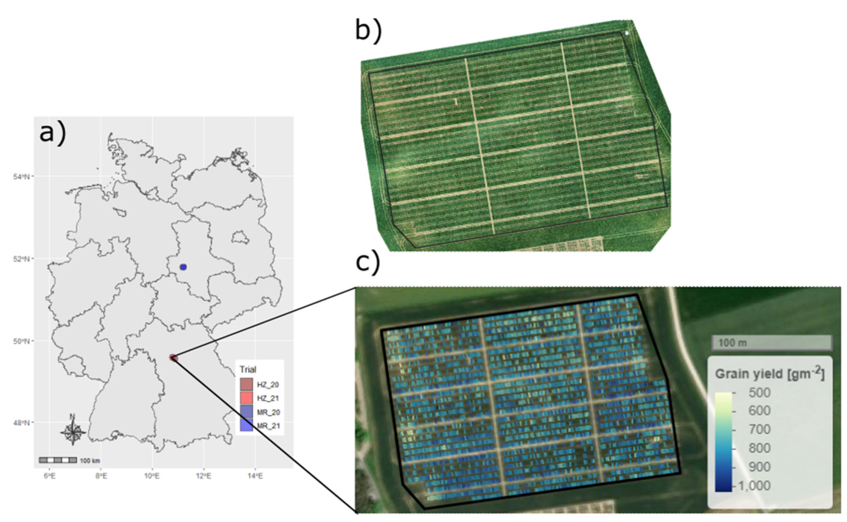
Figure 1. Location of the trials within Germany (a) and overview of the trial: Example of the RGB orthomosaic in HZ_21 on 14 May 2021 (b) and parcel-level grain yield of harvested plots in HZ_21 (c).
Remotesensing 14 06345 g001
Figure 2. R2 values observed using different machine learning algorithms depending on the number of predictors; n = 5790 models from all combinations of times and spectral parameters in all trials. Smoothed curves are based on a generalized additive model.
Remotesensing 14 06345 g002
Figure 3. Comparison of aggregated R2 results (mean and range) by measurement time, compared using Tukey’s HSD post hoc test from the model time*SP (Table S5): Mean values (points) and range (bars). Different group letters and colors denote significantly different values. Dates are indicated as YYYY-MM-DD. ‘MR’ (a,c) and ‘HZ’ (b,d) denote the trial locations, ‘20’ (a,b) and ‘21’ (c,d) the trial years, respectively.
Remotesensing 14 06345 g003
Figure 4. Temporal development of maximum R2 values by spectral parameter (lines) by trial. Line types indicate the sensor (dashed: RGB, continuous: multispectral). In-plot numbers indicate Zadok’s growth stage. Labeled, highlighted lines refer to the overall best spectral parameters for both sensor groups. Dates are indicated as MM-DD. Y-axes are adapted for accounting for the years-specific differing level in prediction accuracies.
Remotesensing 14 06345 g004
Figure 5. Comparison of aggregated coefficient of determination (R2) results by SP, compared using Tukey’s HSD post hoc test from the model time*SP: Mean values (points) and range (bars). Different group letters and colors denote significantly different values. ‘MR’ (a,c) and ‘HZ’ (b,d) denote the trial locations, ‘20’ (a,b) and ‘21’ (c,d) the trial years, respectively.
Remotesensing 14 06345 g005
Figure 6. Comparison of maximum R2 values from individual date models to maximum R2 values from multi-date models by SP and by field trial based on the SVM algorithm. As in Figure 4, the overall best spectral parameters from the RGB and MS camera are labeled.
Remotesensing 14 06345 g006
Table 1. Overview of UAV measurements: Dates (day-month-year), approximate growth stages (Zadok’s scale), and accumulated growing degree days (GDD). GDD is based on local weather data (source: DWD Climate Data Center) with minimum and maximum thresholds of 5 and 30 °C, respectively. Notes: 1: only for reference digital elevation model (DEM); 2: also used for reference DEM model, no DEM data used directly in modeling.
TrialDateGrowth StageGDDNotes
MR_2003 March 2020212561
01 April 202025338
23 April 202030472
08 May 202033574
19 May 202043647
08 June 202072839
24 June 2020751061
09 July 2020831275
HZ_2020 February 2020211371
26 March 202025233
09 April 202030309
06 May 202033516
20 May 202043635
29 May 202065717
08 June 202075812
19 June 202081943
26 June 2020841040
08 July 2020851205
MR_2102 March 2021212132
24 March 202124249
20 April 202130356
28 April 202131389
03 June 202163670
17 June 202172871
06 July 2021791149
20 July 2021851349
HZ_2125 March 2021221902
15 April 202127274
30 April 202133343
14 May 202137422
08 June 202157638
13 July 2021851132
Table 3. Descriptive statistics of plot level grain yield [g m–2] by trial. n: number of plot; SD: standard deviation; C.V.: coefficient of variation.
TrialMeanMinimumMaximumSDCVn
MR_20792223113112616%4423
HZ_20715290103110815%4349
MR_2184930011169111%2787
HZ_218185001027729%2711
Table 4. Aggregated R2 results by machine learning algorithm (MLA), compared using Tukey’s HSD post hoc test from the model MLA*time (Table S3). Grey shades highlight results of the best MLA by trial.
TrialMLAMean R2Maximum R2GroupMean RMSE
[kg plot−1]
Minimum RMSE
[kg plot−1]
MR_20GBM0.510.84ab0.520.32
MLR0.470.81c0.540.33
PLS0.480.82bc0.540.32
RF0.500.85abc0.530.31
Ridge0.480.82bc0.530.32
SVM0.520.84a0.510.31
HZ_20GBM0.470.78a0.450.29
MLR0.420.75c0.480.31
PLS0.440.76abc0.460.30
RF0.460.78ab0.450.29
Ridge0.440.76bc0.470.30
SVM0.460.81ab0.450.27
MR_21GBM0.120.57a0.470.33
MLR0.100.46a0.480.37
PLS0.110.49a0.480.36
RF0.120.57a0.470.33
Ridge0.110.50a0.470.36
SVM0.130.61a0.470.32
HZ_21GBM0.190.41ab0.340.29
MLR0.150.35c0.370.31
PLS0.170.42b0.350.29
RF0.190.41ab0.340.29
Ridge0.170.44b0.340.29
SVM0.190.44a0.340.29
Publisher’s Note: MDPI stays neutral with regard to jurisdictional claims in published maps and institutional affiliations.