The Likely Thermal Evolution of the Irregularly Shaped S-Type Astraea Asteroid

Abstract

The thermal evolution of asteroids provides information on the thermal processes of the protoplanetary disk. Since irregular bodies have a large surface subject to fast heat loss, we used the finite element method (FEM) to explore the likely thermal pathways of one of these bodies. To test our FEM approach, we compared the FEM to another algorithm, the finite difference method (FDM). The results show that the two methods calculated a similar temperature magnitude at the same evolutionary time, especially at the stage when the models had temperatures around 800 K. Furthermore, this investigation revealed a slight difference between the methods that commences with a declining temperature, particularly around the center of the model. The difference is associated with the tiny thickness of the boundary used in the FDM, whereas the FEM does not consider the thickness of the boundary due to its self-adapting grid. Using the shape data provided by DAMIT, we further explored the likely thermal evolution pathway of the S-type asteroid Astraea by considering the radionuclide ²⁶Al. Since we only focused on the thermal pathways of conduction, we considered that the accretion lasts 2.5 Ma (1 Ma = 1,000,000 years) by assuming that Astraea has not experienced iron melting. The results show a high interior temperature area with a shape similar to the shape of Astraea, indicating the influence of the irregular shape on thermal evolution. The interior of Astraea achieved the highest temperature after 4.925 Ma from the accretion of planetesimals. After that time of high temperature, Astraea gradually cooled and existed more than 50 Ma before its heat balanced approximately to its external space. We did not find signs of apparent fast cooling along the shortest z-axis as in previous studies, which could be due to the hidden differences in the distances along the axes. The methodology developed in this paper performs effectively and can be applied to study the thermal pathways of other asteroids with irregular shapes.

1. Introduction

(5) Astraea (hereafter, Astraea) is a large, irregularly shaped asteroid in the main asteroid belt between Mars and Jupiter. The belt survives as a remnant of the protoplanetary disk that formed about 4.56 billion years ago, which is composed of millions of asteroids. Astraea was discovered on 8 December 1845 by the German amateur astronomer Karl Ludwig Hencke [1]. The mass of Astraea was determined to be 2.9 × 10¹⁸ kg using the gravitational perturbations on the orbits of other asteroids [2]. The precise determination of the mass of an asteroid is challenging because the gravitational perturbations of asteroids, especially small ones, are difficult to detect [3]. The mass of Astraea was revised to 2.1674 × 10¹⁸ kg at low accuracy due to its sensitivity to the mass of Juno [4]. Furthermore, this newly updated mass of Astraea was later revised to a less precise, but more probable, value of 2.64 ± 0.44 × 10¹⁸ kg after an analysis of the gravitational effect of the minor planets on other objects [5]. The bulk density and porosity of Astraea can be derived from its volume and mineralogy.

The volume of Astraea was determined using photometric light curves. Based on the prevailing optimization methods for asteroid light curve inversion, as proposed by Kaasalainen and Torppa [6,7], the photometric light curves provided the primary source of information concerning the asteroid shape. The shape of Astraea derived from its light curves can be downloaded from the Database of Asteroid Models from Inversion Techniques (DAMIT: https://astro.troja.mff.cuni.cz/projects/damit/ (accessed on 15 September 2022)) created by Ďurech et al. 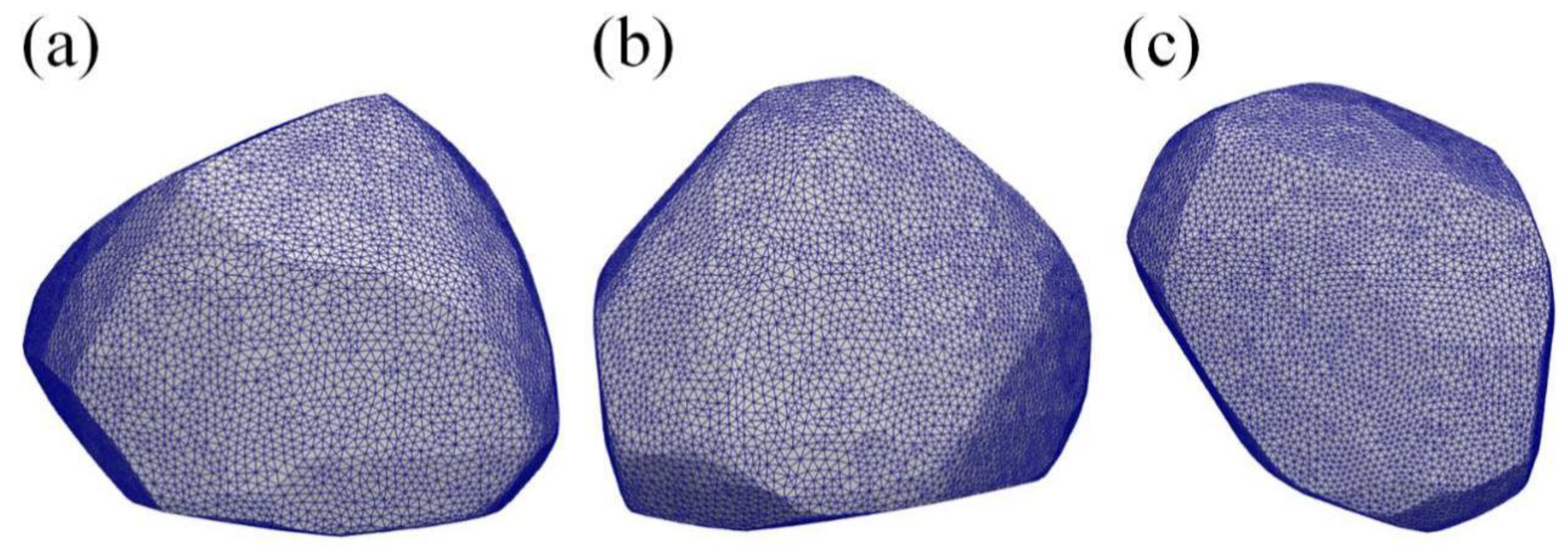[8]. The shape of Astraea downloaded from DAMIT is shown in Figure 1. The spatial grids of this shape are used in our later finite element analysis. Additional resources can be used to further constrain the shape of an asteroid, such as radar data, optical images, and occultation images [9,10]. Using All-Data Asteroid Modeling (ADAM), the mean diameter of Astraea was estimated to be 114 ± 4 km [11], which is consistent with the value of 115 km found in a previous study [5]. The updated bulk density of Astraea was estimated to be around 3.4 g cm⁻³, which is slightly larger than the mean density (~3.26 g·cm⁻³) of an S-type asteroid [12].

The S-type asteroids make up to around 17% of all asteroids in the main belt [12,13]. Like most S-type asteroids, Astraea is likely a mixture of nickel–iron and silicates of magnesium and iron [13]. The main asteroid belt displays a compositional and temperature gradient from its inner to outer parts. The belt provides a record of the decreasing temperature of the protoplanetary disk. The inner region of this disk had a temperature high enough to form solids, whereas the outer more distant part from the proto-Sun is sufficiently cold to give birth to ice and giant gaseous planets [14]. Like other S-type asteroids, Astraea is denser than most of the C-type bodies and experienced a heating process related to radioactive isotope decay. The heating source is mainly ascribed to the short-lived radionuclide ²⁶Al, as inferred by the Ca–Al-rich inclusion (CAIs) found to be widespread in early solar system grains [15]. CAIs are the early condensed first solar system objects and are deciphered to include a canonical initial value of 5 × 10⁻⁵ for ²⁶Al/²⁷Al.

During the early stages of solar nebula evolution, some planetesimals evolved as solid objects in protoplanetary disks to become asteroids. Planetesimals generally experienced collisions owing to gravity perturbations and eventually accreted to form planets. However, some planetesimals escaped accretion and survived as shattered remnants to become the present asteroids [16]. Asteroids thus provide information about the thermal processes of planetesimals in the young Sun’s solar nebula as well as the parent body of asteroids. Most of the planetary bodies are assumed to have spherical shapes [17,18,19]. Unlike spherical models, the real asteroids are mostly non-spherical due to their lack of quasi-hydrostatic equilibrium. Thus, it is necessary to develop thermal models for asteroids with irregular shapes.

Asteroids with irregular shapes have faster interior cooling due to their large surface area [19]. As 3-D (three-dimensional) models have a larger surface-to-volume ratio than their 2-D (two-dimensional) counterparts, 3-D thermal models are more suitable for irregularly shaped objects than 2-D models. Sahijpal [20] recently developed a 3-D thermal model for irregularly shaped objects and found the fastest cooling occurs on the shortest semimajor axis of an ellipsoidal body. Irregular-shaped bodies cool down rapidly due to their large surface area, which allows for more heat loss. To numerically solve the heat conduction equation, Sahijpal tested an explicit 3-D FDM and a fraction-step semi-implicit 3-D Crank–Nicholson method and found these two techniques generated nearly identical results. He further used the explicit 3-D finite difference method to study the possible thermal evolutionary pathways for realistic models of S-type asteroids: (243) Ida and (951) Gaspra. According to Sahijpan [20,21], it is necessary to adopt a suitable choice of temporal and spatial grid intervals to achieve numerical stability. Stability is somewhat difficult to achieve when the thermal diffusivity increases rapidly with the compaction of asteroids due to porosity loss. Although Sahijpan [20,21] introduced a shape generator logic function to construct realistic 3-D physical shapes for asteroids, dealing with the outer surface of an asteroid continues to be complex when special boundary conditions are applied, such as the Neumann condition. The finite element method (FEM), however, can avoid the instability resulting from unreasonable temporal and spatial grids, and can effectively handle complex boundary conditions [22].

Based on the FEM developed in this study, we performed simulations of the thermal evolution of Astraea. The specific onset time of accretion and the thermal dynamic properties of Astraea are not yet known. Therefore, we do not claim to give the exact thermal evolution of the asteroid. Instead, our research focuses on the development of a FEM to model the thermal evolution of a wide-range ensemble of asteroids with irregular shapes. This paper is arranged as follows: the methodology is discussed in Section 2; a comparison between our FEM and a previous FDM is presented in Section 3; the thermal evolutionary pathway is detailed in Section 4; and conclusions drawn from the work are summarized in Section 5.

2. Methodology

2.1. Heat Conduction Equation

Following a previous study, here we considered only the energy produced by the decay of ²⁶Al as the main heat source [23,24], since the in-situ measured composition rate of the specific radionuclide is not available and the energy released by the radionuclide ²⁶Al is larger than other energies such as accretional energy or the heat from long-lived radionuclides. The radionuclide ²⁶Al used here has a decay energy of 3.16 MeV [24]. The radioactive heat generation in an asteroid produces a temperature gradient. The temperature is governed by the heat conductive equation, which uses the parameters that are shown in

Table 1. Values of various parameters used in calculation.

Number	Parameters	Values
1	Density of Astraea ρ	3.4 g·cm−3
2	Decay energy of 26Al [20]	3.16 MeV
3	Initial temperature [21]	250 K
4	Temperature on boundary [20]	200 K
5	Heat production rate Q [20,21]	2.2 × 10−7 W·kg−1
6	Decay constant λ of radionuclide 26Al	0.9366854 Ma−1
7	Heat diffusivity k of the unconsolidated case [24]	6.4 × 10−10 m2 s−1
8	Heat diffusivity k of the consolidated case [21]	6.4 × 10−7 m2·s−1

. The heat conductive equation is expressed as follows:

$$\frac{\partial T}{\partial t}-\nabla \cdot \left(k\nabla T\right)=\frac{Q}{c_p}exp\left(-\lambda t\right)$$

(1)

where T is the temperature both inside and on the surface of the asteroid, t is the thermal evolution time, k is the heat diffusivity, c_p is the heat capacity, Q is the initial heat production rate of the radioactive ²⁶Al, and λ is the decay constant of the radionuclide. The sign ∇ represents the gradient operator and the dot indicates the inner product.

To estimate the temperature with the FEM, the weak form (or integral form) must be obtained for the partial differential equation, which is known as the strong form. Equation (1) is theoretically tenable when any nonvanishing function, h(x,y,z), is multiplied on both sides of Equation (1). To obtain the weak form, the multiplied equation needs to be integrated in the whole domain Ω, of the target asteroid. Using Green’s formula, the weak form of Equation (1) is subsequently written as follows:

$${{\displaystyle \iiint }}_{\Omega }\frac{\partial T}{\partial t}hdV+{{\displaystyle \iiint }}_{\Omega }k\nabla T\cdot \nabla hdV={{\displaystyle \iiint }}_{\Omega }\frac{Q}{c_p}exp\left(-\lambda t\right)hdV+{{\displaystyle ∰}}_{\partial \Omega }\frac{q}{\rho c_p}hdS$$

(2)

where the V and S are the volume and the outer surface of the target asteroid, respectively, q is the heat flux on the outer surface, and $\partial$Ω is the outer surface of the asteroid. The other quantities are as those defined in Equation (1).

To obtain the temperature at any time, a surface boundary condition is needed to start the computation numerically. The surface temperature of some asteroids can reach 245 K [25]. Based on recent studies [20,21], we assumed a constant temperature of 200 K across the outside surface of the target asteroid. The Neumann boundary condition associated with the surficial heat flux, q, was ignored because we considered a constant surficial temperature of 200 K as the Dirichlet boundary condition (or the first-type boundary condition). Therefore, Equation (2) in the numerical simulation was converted into the following form:

$${{\displaystyle \iiint }}_{\Omega }\frac{\partial T}{\partial t}hdV+{{\displaystyle \iiint }}_{\Omega }k\nabla T\cdot \nabla hdV={{\displaystyle \iiint }}_{\Omega }\frac{Q}{c_p}exp\left(-\lambda t\right)hdV$$

(3)

The detailed computation process of the FEM is shown in Appendix A. To numerically solve Equation (3) with the FEM, the heat conductivity and the heat capacity are needed.

2.2. Heat Conductivity and Heat Capacity

Previous studies [26,27] have indicated that the porosity during planetesimals accretion can reach a percentage as high as 50%. At high porosity, heat is transported mainly through radiation, reducing the thermal diffusivity in un-consolidated (or un-sintered) bodies [28]. A small diffusion coefficient slows down the heat transportation outwards, resulting in heat accumulation inside. Then, the interior of un-sintered bodies will be heated rapidly to melt the interior; the bodies will experience compaction and thus lose porosity. The loss of porosity increases the heat diffusivity, leading to rapid cooling. The heat diffusivity is both dependent on temperature and associated with the consolidation of the target asteroid. As in [24], we assume that the heat diffusivity of the un-consolidated asteroid is three orders of magnitude lower than that of a consolidated asteroid. A previous study [29] presented the heat diffusivity for the subsequently consolidated asteroid, and we considered this diffusivity for our study. According to previous studies [20,21,24,27], the compaction of small bodies is activated in the temperature range of 650–700 K. However, it is impossible to perform a gradual compaction using a 3-D model.

As the duration of compaction is no longer than 0.01 Ma, the compaction of an asteroid can be modeled as the rapid resizing of its 3-D spatial grid [24]. In [24], the heat diffusivity in the temperature range of 670–700 K is assumed to increase steadily by three orders of magnitude as compared with that of the un-consolidated case. The increase in the rate of diffusivity is about one order of magnitude per 10 K. Based on the study [21], we assumed the proto-body of Astraea compacted in three steps during its consolidation. The entire body can be finally reduced by a factor of 1.2 in the temperature range of 650–700 K, which means the proto-body compacted by a factor of ~1.06 per 10 K. The heat conductivity is associated with temperature, and the heat capacity is dependent on temperature. According to the study [29], the capacity, c_p, varies between 564 and 826 J·kg⁻¹ in the temperature range of 200–1200 K. We used the formula from the work of Sahijapl [21]. The formula is written as follows:

$$c_p=A+B\cdot exp(-0.0036\cdot T)$$

(4)

where A and B have values of 280 and 553 J·kg⁻¹, respectively. The unit of the constant 0.0036 is K⁻¹.

For asteroids, the time of accretion (i.e., t_onset) is greater than 0.7–2.7 Ma after condensation of Ca–Al-rich inclusion with an initial value of 5 × 10⁻⁵ for ²⁶Al/²⁷Al [20]. The onset time of accreted planetesimals greatly affects the final thermal evolution associated with wide-spread melting and differentiation [24,30]. Sahijpal discovered that an eventually generated body with a radius around 270 km needs an accretion time of about 1 Ma in duration to generate significant melting and differentiation. Sugiura and Fujiya [30] found that the ordinary and carbonaceous chondrites accreted in about 2–3 Ma. Our study addresses the likely thermal metamorphism without huge melting and differentiation; the time of accretion of planetesimals was thus set in the range 1.5–3 Ma.

2.3. Development of Shape Generator Function

The FDM developed by Sahijpal was used to study asteroids including (951) Gaspra and (243) Ida [21]. Sahijpal developed a shape generator logical function to confine the asteroid shape in a cubic form. The generator function G(x,y,z) (or a matrix) is written as follows:

$$G\left(x,y,z\right)=\left\{\begin{array}{c}1\\ 0\end{array}\right. \begin{array}{c}\left(r\le r_s\right)\\ \left(r>r_s\right)\end{array}$$

(5)

where r is the radius of a point A in the real asteroid and r_s is the radius of a point B on the boundary. For any point A(x_A,y_A,z_A), we can compute its radius, r, to the asteroid’s center and calculate its geographic latitude ϕ and longitude θ. Using the same geographic coordinates (ϕ,θ), we can obtain the radius, r_s, of a point on the boundary of the asteroid. Using the function in Equation (5), we can determine whether point A is outside of the asteroid or not. The quantity G equaling to zero means the location outside of asteroid; whereas G = 1 indicates the point in the interior of the body or on the boundary.

In the actual process of temperature estimation, we need to evaluate the temperature in a whole cube, and subsequently confine the temperature distribution with the logical shape generator function G. To deal with boundary conditions, we developed a boundary shape function G_b(x,y,z) to simplify the computation, which is written as follows:

$$G_b\left(x,y,z\right)=\left\{\begin{array}{c}1\\ 0\end{array}\right. \begin{array}{c}\left(\left|r-r_s\right|\le \epsilon \right)\\ \left(\left|r-r_s\right|>\epsilon \right)\end{array}$$

(6)

where ε is a tolerance quantity that is assumed to be zero. However, the quantity ε cannot approach zero due to the limited spatial resolution. The temperature T(x,y,z) in the whole cube can be confined according to the shape functions G and G_b as follows:

$$T=T_s\cdot G_b+T_0\cdot G\cdot \left(1-G_b\right)$$

(7)

where the black dot is the dot product between two matrixes and T_s and T₀ are the surficial temperature of an asteroid and the previous temperature at the last time-step, respectively. The first part in the sum of Equation (7) signifies the temperature distribution on the boundary; the last term represents the temperature distribution in the interior of an asteroid.

3. Comparison of Results between FDM and FEM

To validate our methodology, we tested the thermal evolution obtained using our approach. We studied the thermal evolution of a spherically shaped asteroid and compared the results obtained using the FDM and the FEM. The FDM cannot easily deal with boundary conditions. We assume that the grid intervals of the three axes (e.g., x, y, and z) are denoted by Δx, Δy, and Δz. According to a previous study [20], the convergence of the FDM depends on the stability factor, $R=\frac{k\Delta t}{{\Delta x}^2}=\frac{k\Delta t}{{\Delta y}^2}=\frac{k\Delta t}{{\Delta z}^2}$, which is supposed to be lower than 0.5. A small value of ε means small spatial grids, thus indicating a high resolution of spatial grids. Therefore, a small ε in Equation (6) will amplify the stabilizing factor, R, leading to FDM divergence. To stabilize the FDM, we used a tradeoff where ε was close to 0.025 to ensure an R approaching 0.202, which is lower than 0.5. Consequently, we apply a spatial grid of Δx = Δy = Δz = 0.25. To validate our approach, we considered a spherically shaped asteroid with a radius of 35 km. 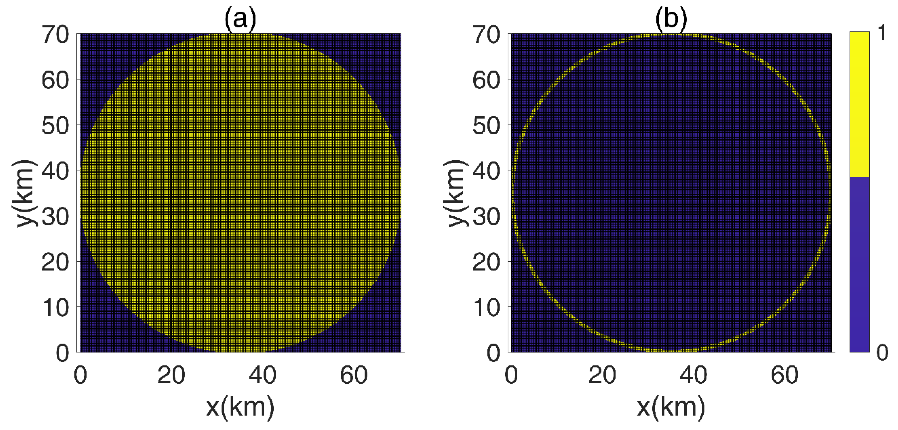Based on a previous study [20], we used the constant heat diffusivity k = 8 × 10⁻⁷ m²·s⁻¹. The temperature-dependent heat capacity was estimated according to Equation (4). According to Equations (5) and (6), we constructed a shape function, G(x,y,z), and a boundary shape function, G_b(x,y,z), to confine the temperature estimated by the FDM. These two shape functions are shown in Figure 2, where the background nets provide the FDM grids used in temperature calculations.

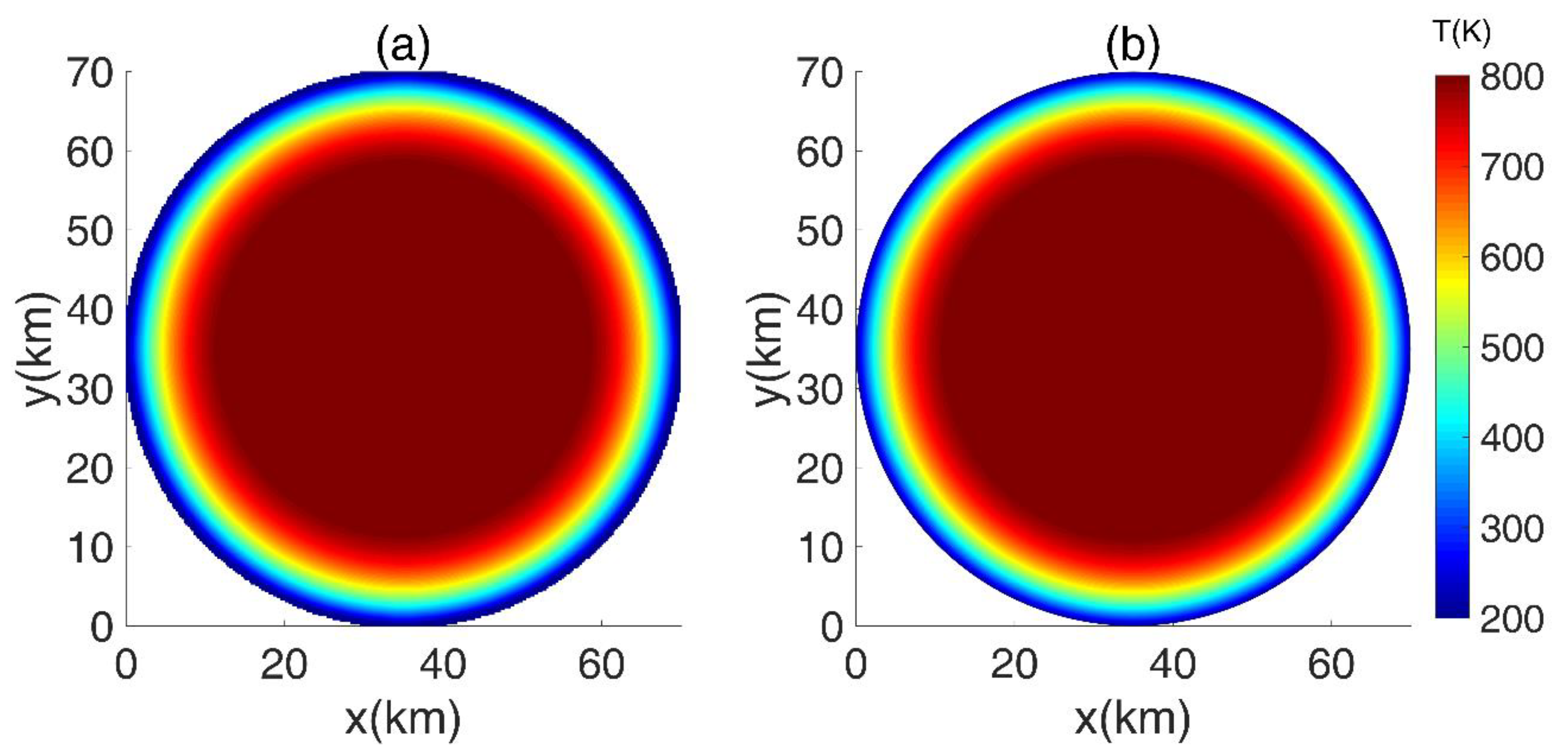
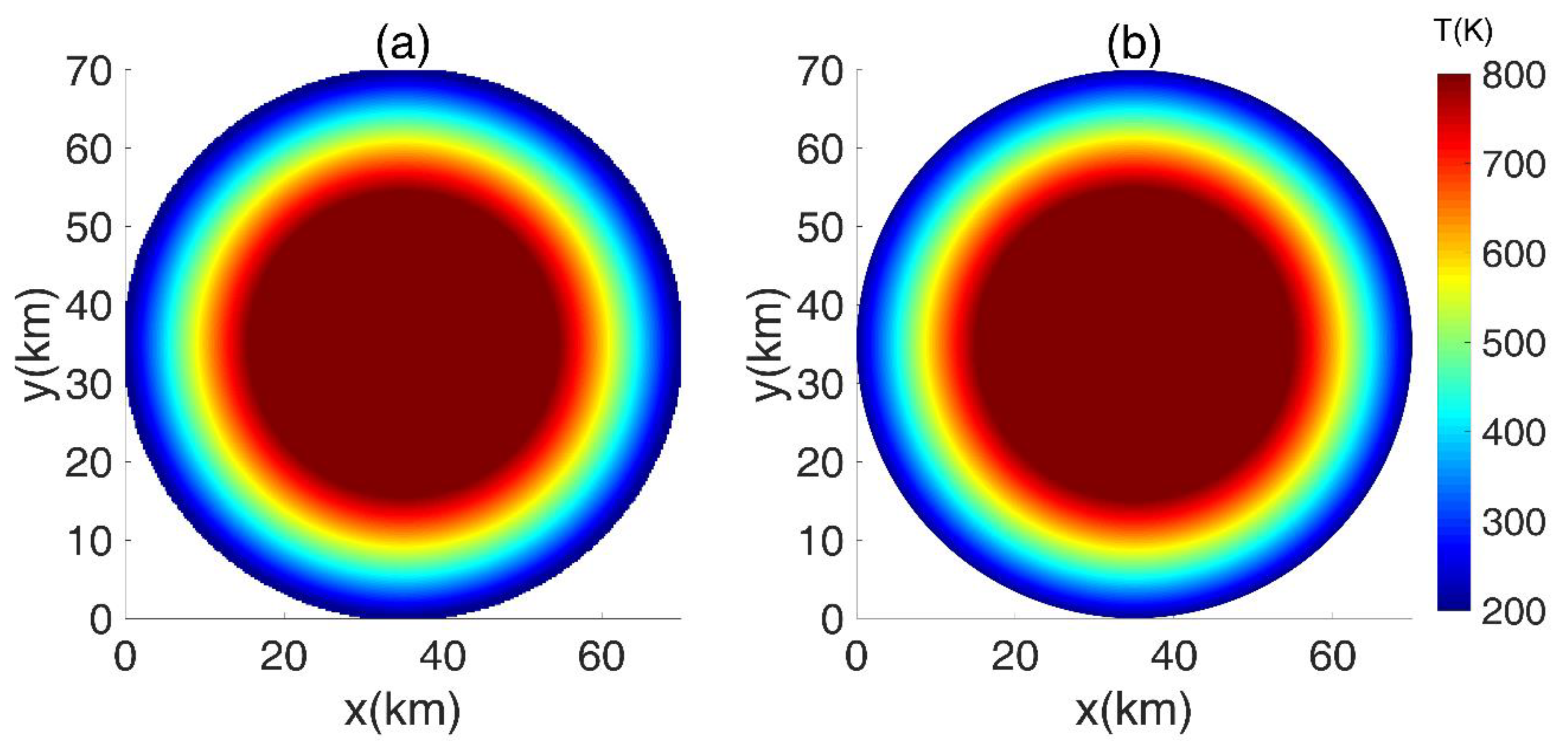
According to a previous study [20], the time of accretion, t_onset, of planetesimals to a proto-asteroid is between 1.5 and 3 Ma. We considered the short-lived radionuclide ²⁶Al as the sole heating source, and thus chose the time t_onset = 2.5 Ma in our study. Figure 3 gives the sectional temperature of the x-y plane at the time t = 3.5 Ma.

The two sub-figures 3a and 3b depict the results of FDM and FEM, respectively. A hot area was observed at the center, and a cold circle was observed on the boundary. The temperature in the center reached 800 K, whereas the boundary temperature stayed around 200 K due to the fixed Dirichlet boundary condition. Both figures show the same temperature magnitude and distribution. Compared with the temperatures shown in Figure 3, Figure 4 depicts the reduced size of the high temperature area after 5 Ma from the accretion.

The two sub-figures 4a and 4b illustrate a similar variation in temperature. From the results shown in Figure 3 and Figure 4, it can be concluded that the FEM results are generally consistent with those from the FDM, indicating the feasibility of our algorithm. As heat is lost from the asteroid, the thermal energy from the decaying radionuclide ²⁶Al is not sufficient to further heat the interior of the body. 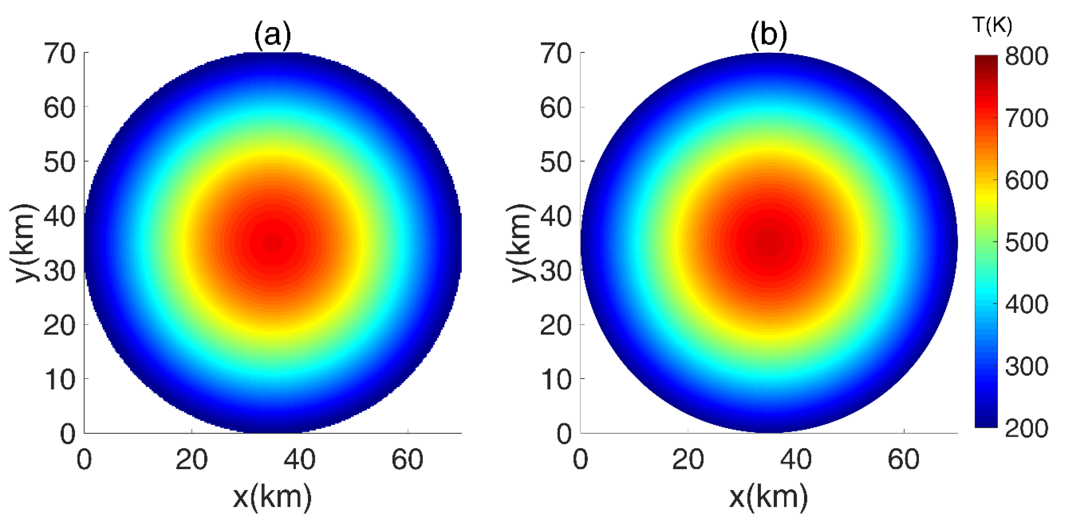The temperature decreases over time as presented in Figure 5 and Figure 6.

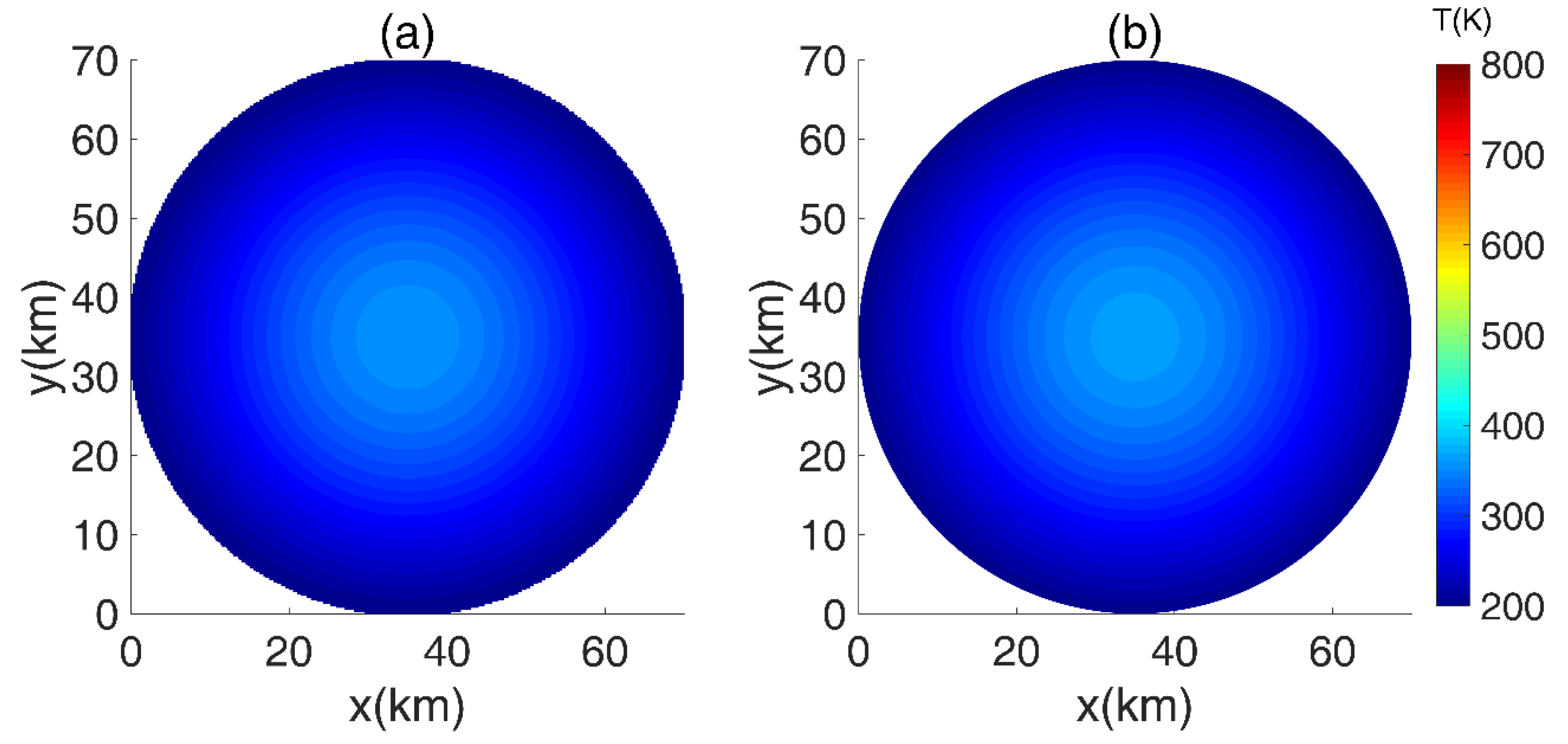
Figure 5 demonstrates that the size of the hot area further decreases so that the maximum temperature is reduced to around 700 K after 10 Ma from accretion. Although the two sub-figures 5a and 5b show similar results, there is a slight difference in the centers which displayed hot areas. Figure 5b shows a slightly larger hot center than that shown in Figure 5a. Figure 6 shows the temperature distribution after 20 Ma from accretion. Figure 6 indicates that the interior of the asteroid continues to lose heat and that the maximum temperature is confined to 400 K. The two sub-figures 6a and 6b show the same variation in temperature, but there is a small difference in the center of the body. Figure 6a indicates that the maximum temperature in the center of the body is within 360 K, whereas Figure 6b shows a maximum value of 380 K in the center. This discrepancy could likely be due to the limited size of the boundary thickness in the FDM. The FDM is theoretically supposed to have a boundary with a tiny thickness. However, the limited spatial grid space (Δx = Δy = Δz = 0.25) cannot further reduce the modeled thickness of the asteroid’s surface boundary. Figure 2b shows the distribution of the boundary, which is clearly thick. Conversely, the FEM does not limit the thickness of the boundary due to the self-adapting grid. Figure 7 shows the FEM grid on the x-y plane, where the boundary is represented by the nodes in the boundary grids.

Figure 7 shows that the FEM can more effectively deal with the boundary condition than the FDM because the physical boundary is well represented by the lines of the FEM grids on the boundary. We subsequently used the FEM to study the likely thermal evolution of the irregularly shaped Astraea.

4. Thermal Evolution of the S-Type Asteroid Astraea

After testing the FEM, we applied the approach to study the likely thermal evolution of Astraea. Using the shape of Astraea, we fixed its surface temperature to a constant value of 200 K. Based on a previous study [20], we assumed the accretion of planetesimals lasted 2.5 Ma. We also tested the short case of t_onset = 1.5 Ma and found the maximum temperature increased to more than 1500 K. Iron melting would commence at that temperature, but discussing this scenario is out of the scope of this study. 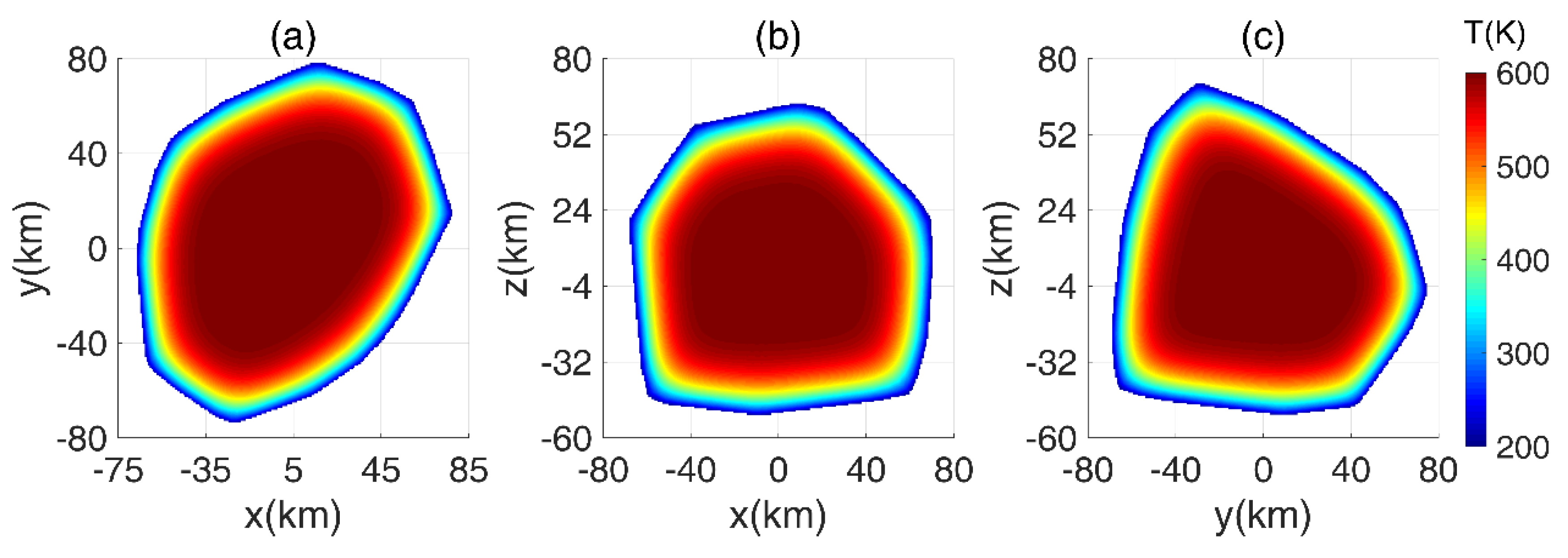After dozens of tests and referring to a previous study [20], we assumed the accretion lasted 2.5 Ma (i.e., t_onset = 2.5 Ma), and found the likely temperature contours after 0.46 Ma, as shown in Figure 8.

The two sub-figures 8a and 8b illustrate the sectional temperature variations along the x-y plane and the x-z plane. The two figures indicate a high temperature close to 600 K in a large part of the interior, whereas the surface is cold at 200 K due to the fixed surface temperature. Figure 8c shows the temperature distribution along the y-z plane, and indicates a similar magnitude of temperature to those in Figure 8a,b. A maximum temperature lower than 700 K indicates that the body is not yet un-consolidated. 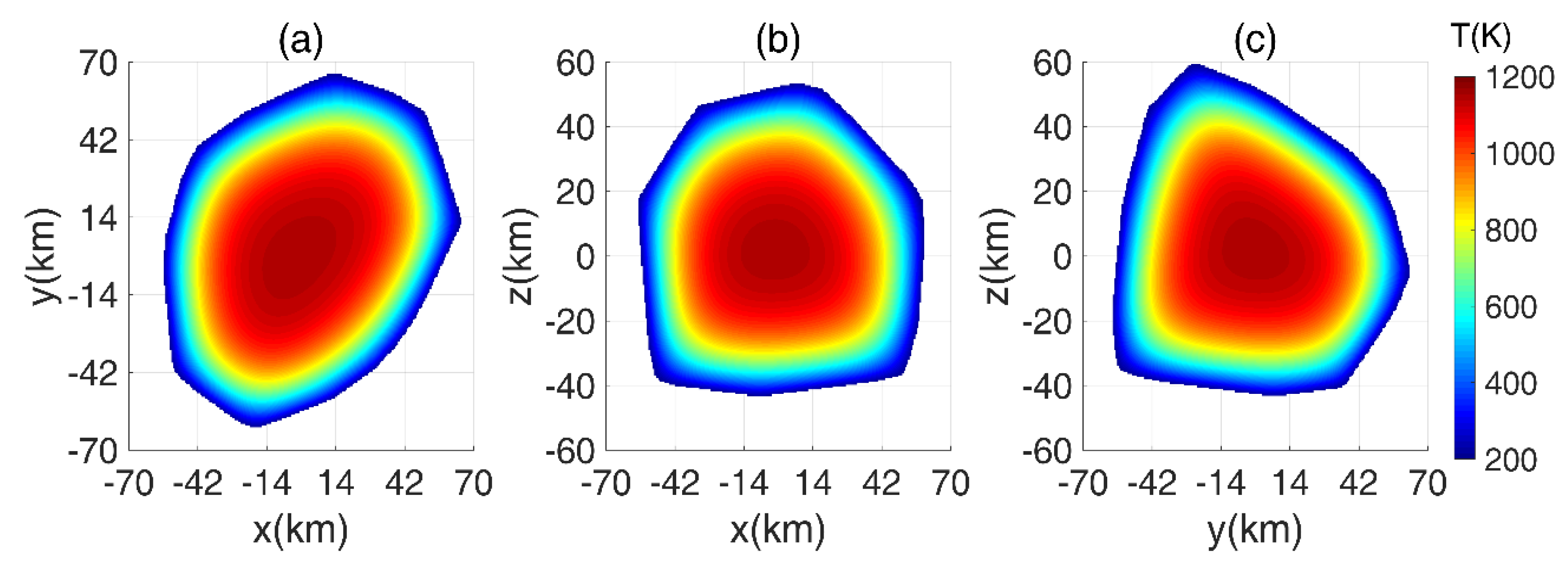The body will continue to heat up due to the radioactive decay of ²⁶Al. By the end of the accretion of planetesimals, the body will have spent 4.925 Ma being heated to a high temperature such as those seen in Figure 9.

Figure 9a–c indicate that a large part of the interior of Astraea is heated to a temperature greater than 1000 K, whereas the center of the body can rise up to 1150 K. The shape of the high temperature at the interior is to some extent similar to the shape of Astraea, but the interior is smoother than the surface shape. Comparing the grids shown in Figure 8 and Figure 9, the grid limitations in Figure 9 are smaller than those shown in Figure 8. Since the compaction of an asteroid commences at around a temperature of 700 K [24], the body experienced consolidation at the time t = 7.425 Ma. Following previous studies [20,24], we assumed the body experienced reduction in three steps by a factor of ~1.06 in the temperature range of 670–700 K. The initial spatial grids were compacted by a factor of 1.2 to generate the final grids. 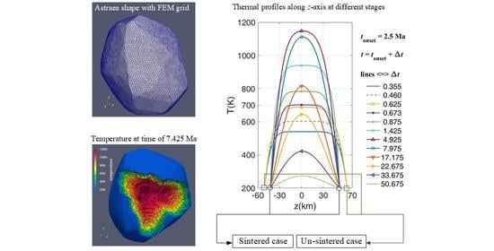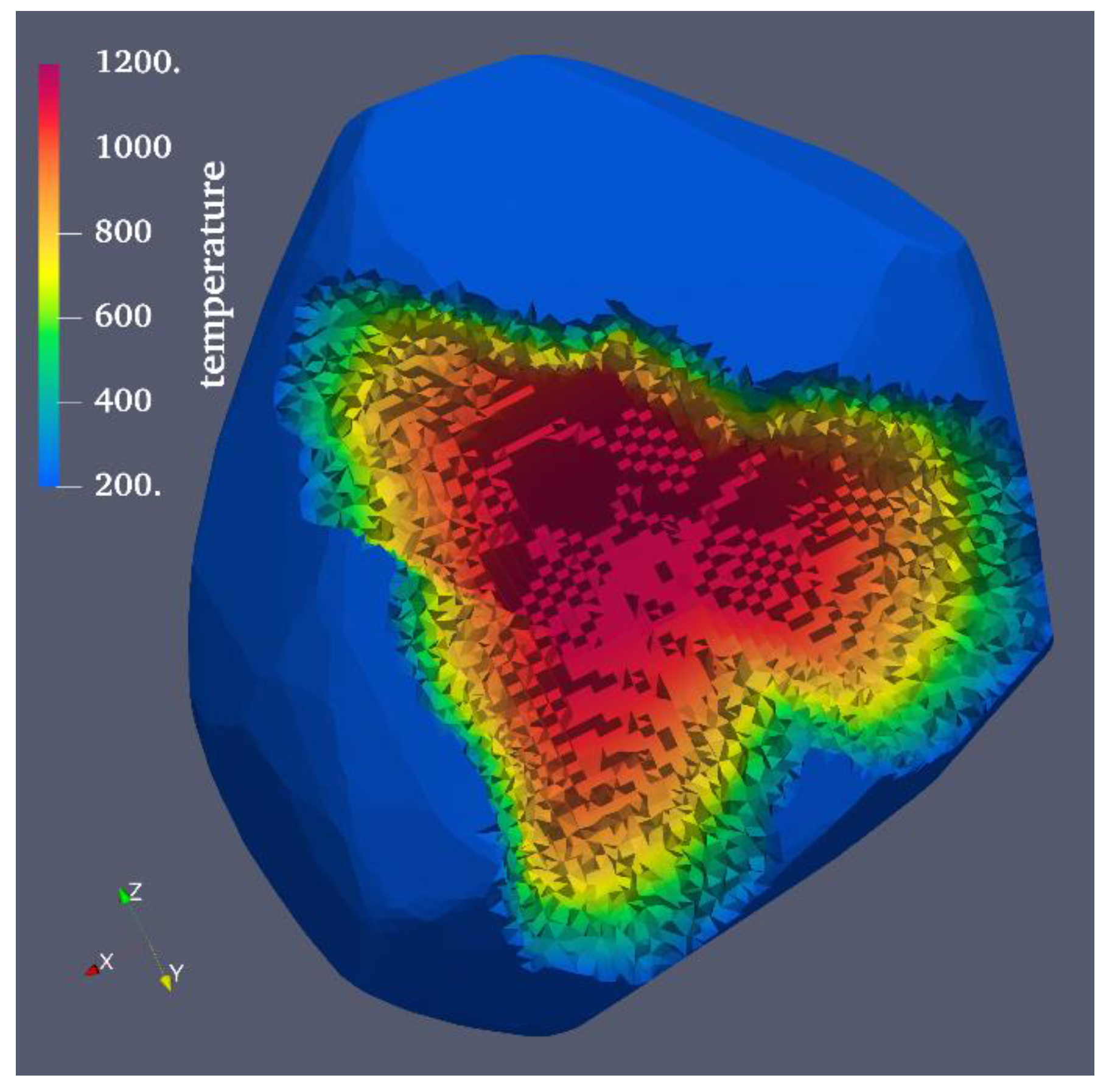The grids shown in Figure 9 are thus smaller than those in Figure 8 by a factor of ~1.2. Additionally, we provide a stereogram of the temperature distribution at time 7.425 Ma, as shown in Figure 10.

To display the temperature contours of the interior, we made a gap on the surface as shown in Figure 10. The rough grains in the interior represent the geometrical elements used in the FEM. Viewing through the gap we found that the temperature of the interior, especially around the body’s center, is close to a high value of 1200 K. As the heat conducts from the interior to the outer surface, the temperature decreases gradually to 200 K on the surface. With the loss of heat, the body cooled gradually after 7.425 Ma. 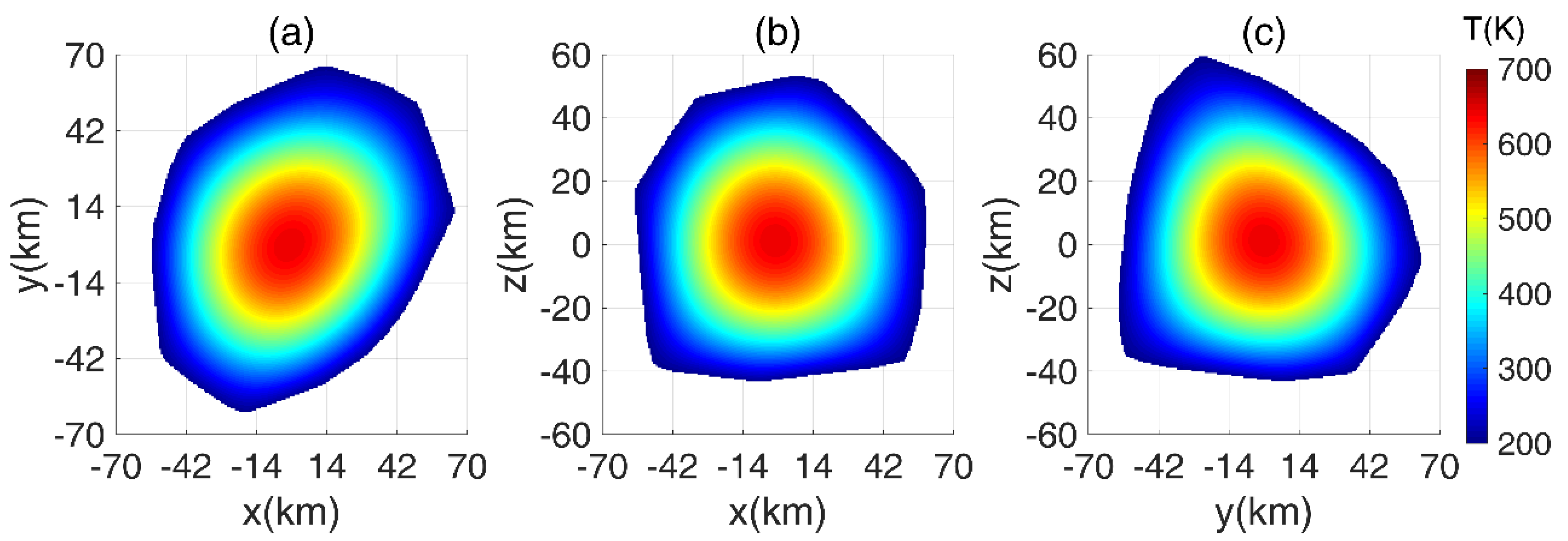Until 25.175 Ma, the interior of the body cooled as shown in Figure 11.

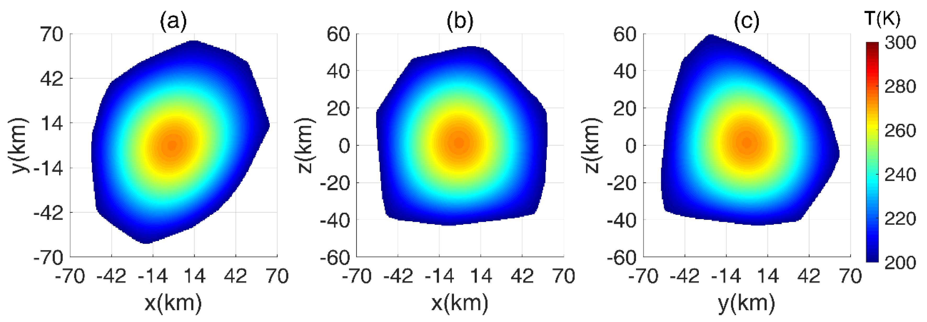
Figure 11 indicates that the temperature in the body’s center is less than 700 K. The size of high temperature area is smaller than in the previous period. There are regions near the boundary with low temperatures of around 300 K. After 50.675 Ma from accretion, the interior of the body further cooled, and the temperature decreased to lower than 300 K, as in Figure 12.

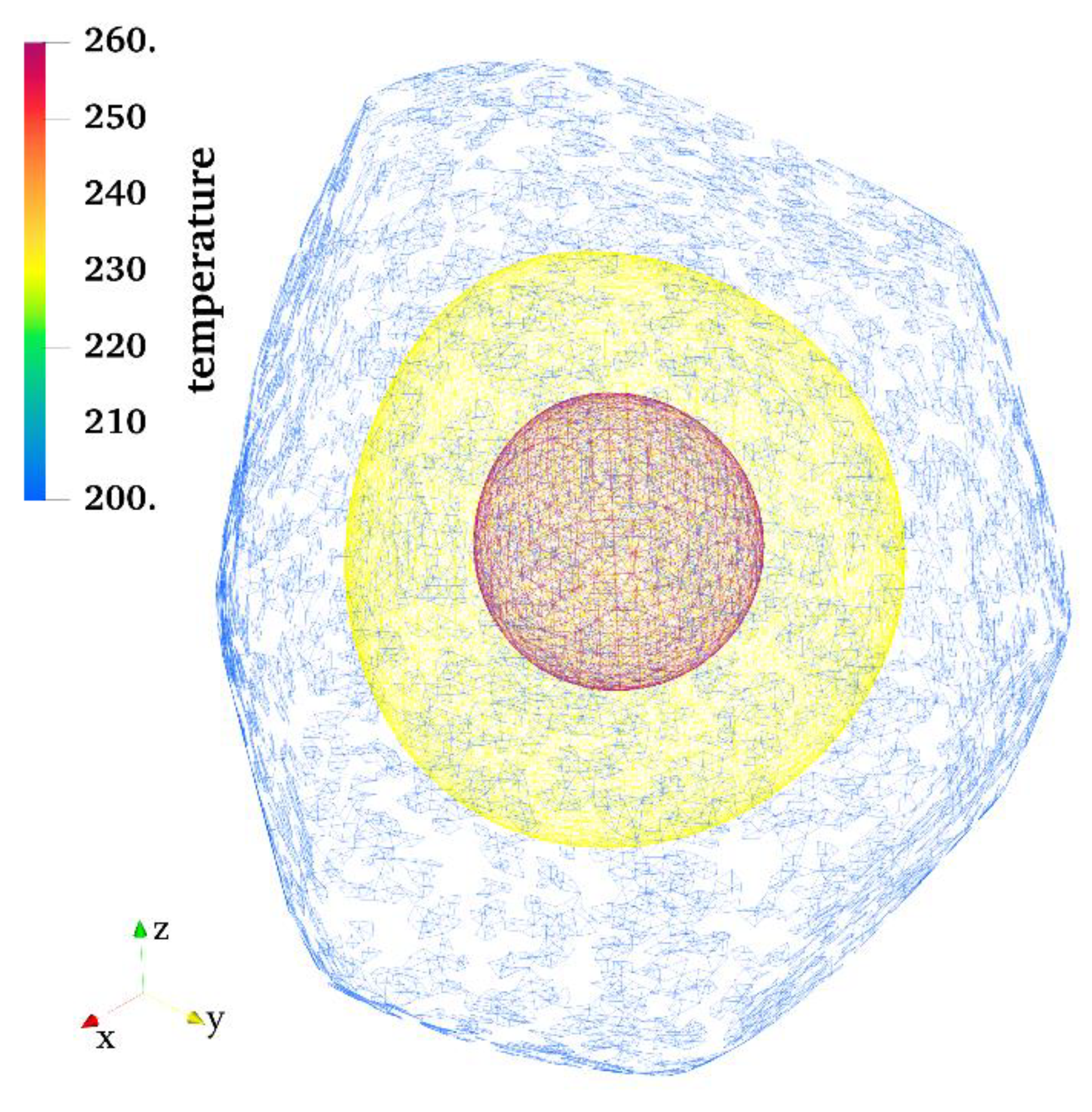
Figure 12a–c show that the high temperature area is concentrated around the center and has a temperature of around 260 K. Figure 13 presents a stereogram of the temperature distribution of this feature with three iso-surfaces.

As seen in Figure 13, the three iso-surfaces from the outer surface to the inner surface represent temperatures of 200 K, 230 K, and 260 K. The inner iso-surface appears as a small red sphere, indicating the body cooled to be approximately heat balanced with the external space. The temperature gradient declined as the temperature decreased. Thus, the heat loss occurred more slowly than in the case of the high temperature state. 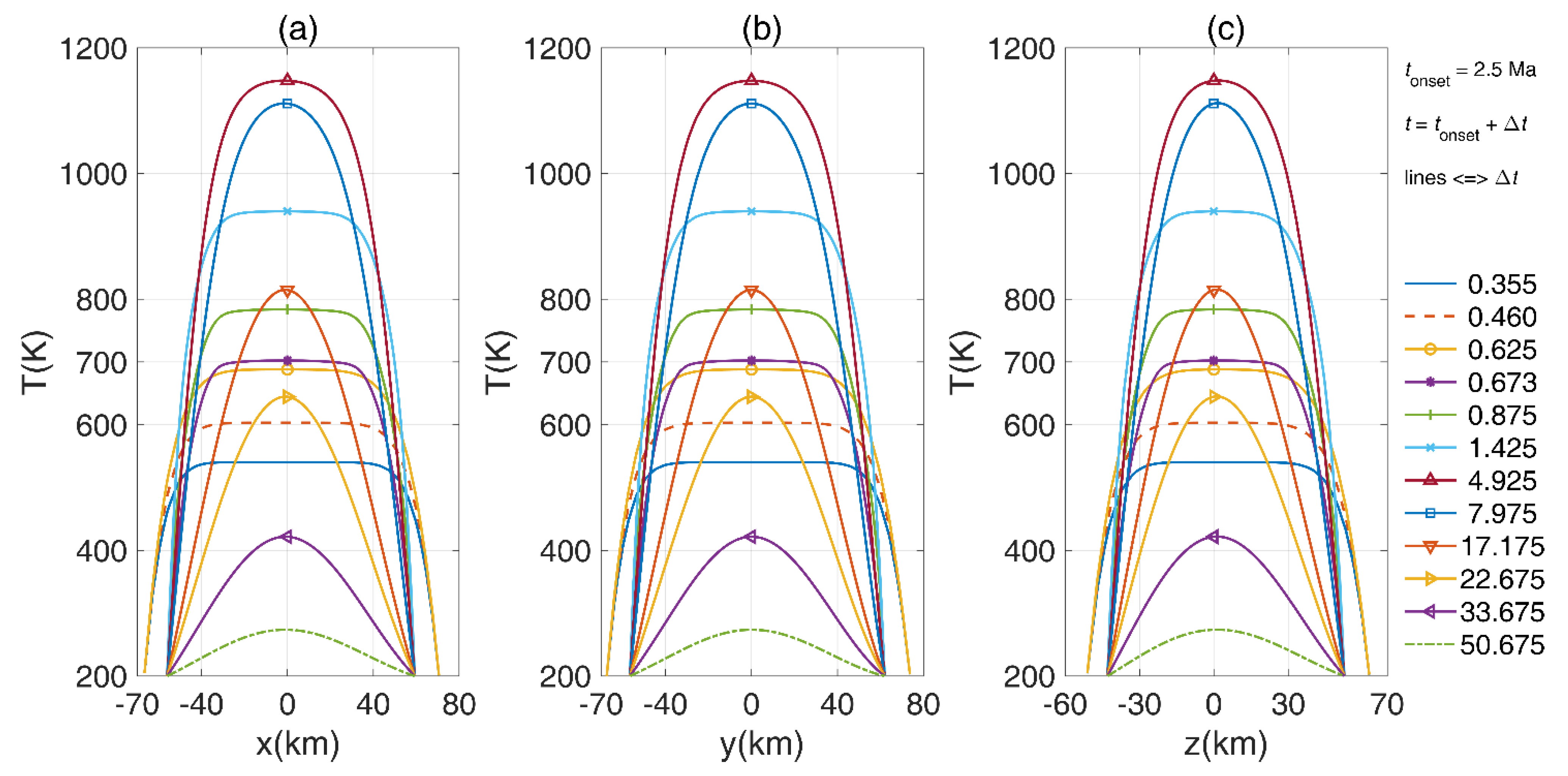Figure 14 gives the thermal profiles along the x-axis (a), y-axis(b), and z-axis (c).

The curves in the panels of Figure 14 represent temperature variation at various stages after the accretion of planetesimals (t_onset=2.5 Ma). After accretion at 0.355 Ma, the solid blue curves in the three panels indicate that the interior of the body heated to 540 K. Figure 14a demonstrates that the distance along the x-axis is around 136.8 km, close to the distance (~140 km) along y-axis shown in Figure 14b. Figure 14c shows the shortest distance along z-axis, where the distance approaches 113 km. Since the maximum temperature is lower than 700 K, the target asteroid did not experience consolidation. The un-consolidated state continues to the time of 0.46 Ma based on the brown curves in the three panels of Figure 14, which indicate that the interior of Astraea heated to 600 K. As the interior of the target body was further heated by radioactive decay, the solid orange lines with circles in the three panels depict that the interior of Astraea further heated to 688 K after 0.625 Ma, indicating that the body was experiencing compaction or consolidation due to porosity loss. Subsequent to accretion after 0.625 Ma, the solid purple curves with asterisks in Figure 14 show that the interior of the target body heated to 701 K, and slightly higher than 700 K. The slightly higher temperature indicates the end of compaction; thus, the distances were shortened along the three axes after that time. The distance along the x-axis in Figure 14a shortened from 136.8 km to around 114 km, whereas the distance along the y-axis in Figure 14b shortened from 140.8 km to nearly 117 km. The distance decreased from 113 km to around 94 km along the z-axis, as shown in Figure 14c. Although the target asteroid experienced consolidation after 0.625 Ma, its interior continued to heat up to a high temperature due to radioactive activity during the following stages.

The solid brown curves with an upper triangle in Figure 14 indicate that the interior of the target body was heated to the maximum temperature close to 1150 K after the time of 4.925 Ma. The maximum value of 1150 K is the largest temperature in our model; thus, the body did not experience iron melting in our computation. After the warmest state, the body in the following periods cooled down due to insufficient radioactive decay energy from ²⁶Al. Until to the time t = t_onset + 50.675 Ma = 53.175 Ma, the dashed green curves in the three panels of Figure 14 indicate the body cooled down sharply and that the temperature of the interior was around 260 K. Although the thermal profile along the z-axis is slightly distinct with those along the x- and y-axes in Figure 14, we did not find an apparent fast cooling with respect to the cooling rate in the shortest z-axis, which was found in a previous study [21]. This slowly cooling rate is likely associated with the unapparent differences in the distances along z-axis and the x- and y-axes in Astraea. However, the distances along z-axis are much smaller than the other two axes in the asteroid (243) Ida as previously studied.

5. Conclusions

Most asteroids are shattered remnants resulting from planetesimals that escaped from protoplanet accretion. Studying the thermal pathways of asteroids can help to understand the thermal processes of the planetesimals in the young Sun’s solar nebula. Modeled asteroids are generally supposed to have regular shapes; however, most real asteroids have irregular shapes due to their lack of quasi-hydrostatic equilibrium. The irregular shapes have larger surface areas than regular models. Large surfaces result in faster cooling than regular models. Although previous research has explored the thermal pathways of irregular shapes of asteroids using the FDM, it is a quite complex task to achieve stability and to deal with boundary conditions using the FDM. To explore the likely thermal pathways of irregular shapes of asteroids, we developed a FEM to infer the thermal evolution of the irregularly shaped Astraea asteroid.

We made a comparison of thermal results from the FDM and the FEM by considering a spherical model with a radius close to 35 km. The two algorithms gave similar results for the same evolutionary time, especially at the stage when the models had temperatures around 800 K. However, the two methods showed a slight difference in temperature owing to heat loss because the FDM is unlikely to achieve a thin boundary. Conversely, the FEM does not consider the thickness of boundary due to its self-adapting grid. Based on the shaped data provided by DAMIT, we further explored the likely thermal evolution pathway of the Astraea S-type asteroid. To explore the likely thermal pathway, we considered the accretion lasting 2.5 Ma to prevent iron melting in the target body and accounted for consolidation owing to porosity loss.

The results show that the shape of the high temperature area in the interior is similar to the shape of Astraea, indicating the influence of the irregular shape on thermal evolution. After the accretion of planetesimals, the interior of Astraea spent 4.925 Ma reaching a high temperature of nearly 1150 K. Subsequently, Astraea gradually cooled due to insufficient radioactive isotope decay and required more than 50 Ma to approximately balance heat to its external space. In addition, we did not find signs of fast cooling in the shortest z-axis as reported in a previous study. This can likely be ascribed to the unapparent differences of distances along the axes of Astraea. This methodology can be applied to the thermal pathways of other irregularly shaped asteroids given the advantages of the FEM as developed in this study.

References

1. Ferguson, J. Observations of (31) Euphrosyne, (8) Flora, (9) Metis, (5) Astraea, (14) Irene, (18) Melpomene, and the thirty-fourth asteroid. Astron. J. 1855, 4, 89–91. [Google Scholar] [CrossRef]
2. Michalak, G. Determination of asteroid masses-II. (6) Hebe, (10) Hygiea, (15) Eunomia, (52) Europa, (88) Thisbe, (444) Gyptis, (511) Davida and (704) Interamnia. Astron. Astrophys. 2001, 374, 703–711. [Google Scholar] [CrossRef]
3. Galád, A. Asteroid candidates for mass determination. Astron. Astrophys. 2001, 370, 311–319. [Google Scholar] [CrossRef] [Green Version]
4. Baer, J.; Chesley, S.R.; Matson, R.D. Astrometric masses of 26 asteroids and observations on asteroid porosity. Astron. J. 2011, 141, 143. [Google Scholar] [CrossRef]
5. Carry, B. Density of asteroids. Planet. Space Sci. 2012, 73, 98–118. [Google Scholar] [CrossRef] [Green Version]
6. Kaasalainen, M.; Torppa, J. Optimization methods for asteroid lightcurve inversion: I. shape determination. Icarus 2001, 153, 24–36. [Google Scholar] [CrossRef]
7. Kaasalainen, M.; Torppa, J.; Muinonen, K. Optimization methods for asteroid lightcurve inversion: II. The complete inverse problem. Icarus 2001, 153, 37–51. [Google Scholar] [CrossRef]
8. Ďurech, J.; Sidorin, V.; Kaasalainen, M. DAMIT: A database of asteroid models. Astron. Astrophys. 2010, 513, A46. [Google Scholar] [CrossRef]
9. Kaasalainen, M.; Viikinkoski, M. Shape reconstruction of irregular bodies with multiple complementary data sources. Astron. Astrophys. 2012, 543, A97. [Google Scholar] [CrossRef] [Green Version]
10. Viikinkoski, M.; Kaasalainen, M.; Ďurech, J. ADAM: A general method for using various data types in asteroid reconstruction. Astron. Astrophys. 2015, 576, A8. [Google Scholar] [CrossRef]
11. Hanuš, J.; Viikinkoski, M.; Marchis, F.; Ďurech, J.; Kaasalainen, M.; Delbó, M.; Herald, D.; Frappa, E.; Hayamizu, T.; Kerr, S.; et al. Volumes and bulk densities of forty asteroids from ADAM shape modeling. Astron. Astrophys. 2017, 601, A114. [Google Scholar] [CrossRef] [Green Version]
12. Vernazza, P.; Ferrais, M.; Jorda, L.; Hanuš, J.; Carry, B.; Marsset, M.; Brož, M.; Fetick, R.; Viikinkoski, M.; Marchis, F.; et al. VLT/SPHERE imaging survey of the largest main-belt asteroids: Final results and synthesis. Astron. Astrophys. 2021, 654, A56. [Google Scholar] [CrossRef]
13. McClure, L.T.; Lindsay, S.S. A contemporary view of the ordinary chondrite boot II: Mineralogical variation of S-type asteroids. Icarus 2022, 379, 114944. [Google Scholar] [CrossRef]
14. Michel, P. Formation and physical properties of asteroids. Elements 2014, 10, 19–24. [Google Scholar] [CrossRef]
15. MacPherson, G.J.; Davis, A.M.; Zinner, E.K. The distribution of aluminum-26 in the early solar system—A reappraisal. Meteoritics 1995, 30, 365–386. [Google Scholar] [CrossRef]
16. Bottke, W.F., Jr.; Durda, D.D.; Nesvorný, D.; Jedicke, R.; Morbidelli, A.; Vokrouhlický, D.; Levison, H. The fossilized size distribution of the main asteroid belt. Icarus 2005, 175, 111–140. [Google Scholar] [CrossRef]
17. Harrison, K.P.; Grimm, R.E. Thermal constraints on the early history of the H-chondrite parent body reconsidered. Geochim. Cosmochim. Acta 2010, 74, 5410–5423. [Google Scholar] [CrossRef]
18. Neumann, W.; Henke, S.; Breuer, D.; Gail, H.-P.; Schwarz, W.H.; Trieloff, M.; Hopp, J.; Spohn, T. Modeling the evolution of the parent body of acapulcoites and lodranites: A case study for partially differentiated asteroids. Icarus 2018, 311, 146–169. [Google Scholar] [CrossRef]
19. Golabek, G.J.; Bourdon, B.; Gerya, T.V. Numerical models of the thermomechanical evolution of planetesimals: Application to the acapulcoite-lodranite parent body. Meteorit. Planet. Sci. 2014, 49, 1083–1099. [Google Scholar] [CrossRef]
20. Sahijpal, S. Thermal evolution of non-spherical asteroids in the early solar system. Icarus 2021, 362, 114439. [Google Scholar] [CrossRef]
21. Sahijpal, S. Possible thermal evolutionary pathways of irregular shaped small asteroids and planetesimals. J. Earth Syst. Sci. 2022, 131, 1–15. [Google Scholar] [CrossRef]
22. Hirabayashi, M.; Kim, Y.; Brozović, M. Finite element modeling to characterize the stress evolution in asteroid (99942) Apophis during the 2029 Earth encounter. Icarus 2021, 365, 114493. [Google Scholar] [CrossRef]
23. Weidenschilling, S.J. Accretion of the asteroids: Implications for their thermal evolution. Meteorit. Planet. Sci. 2019, 54, 1115–1132. [Google Scholar] [CrossRef]
24. Sahijpal, S.; Soni, P.; Gupta, G. Numerical simulations of the differentiation of accreting planetesimals with 26Al and 60Fe as the heat sources. Meteorit. Planet. Sci. 2007, 42, 1529–1548. [Google Scholar] [CrossRef]
25. Coradini, A.; Capaccioni, F.; Erard, S.; Arnold, G.; De Sanctis, M.C.; Filacchione, G.; Tosi, F.; Barucci, M.A.; Capria, M.T.; Ammannito, E.; et al. The surface composition and temperature of asteroid 21 Lutetia as observed by Rosetta/VIRTIS. Science 2011, 334, 492–494. [Google Scholar] [CrossRef] [Green Version]
26. Henke, S.; Gail, H.P.; Trieloff, M. Thermal evolution and sintering of chondritic planetesimals-III. Modelling the heat conductivity of porous chondrite material. Astron. Astrophys. 2016, 589, A41. [Google Scholar] [CrossRef]
27. Henke, S.; Gail, H.P.; Trieloff, M.; Schwarz, W.H.; Kleine, T. Thermal evolution and sintering of chondritic planetesimals. Astron. Astrophys. 2012, 537, A45. [Google Scholar] [CrossRef] [Green Version]
28. Schröder, S.E.; Poch, O.; Ferrari, M.; De Angelis, S.; Sultana, R.; Potin, S.M.; Beck, P.; De Sanctis, M.C.; Schmitt, B. Dwarf planet (1) Ceres surface bluing due to high porosity resulting from sublimation. Nat. Commun. 2021, 12, 274. [Google Scholar] [CrossRef]
29. Yomogida, K.; Matsui, T. Physical properties of ordinary chondrites. J. Geophys. Res. Solid Earth 1983, 88, 9513–9533. [Google Scholar] [CrossRef]
30. Sugiura, N.; Fujiya, W. Correlated accretion ages and ε54Cr of meteorite parent bodies and the evolution of the solar nebula. Meteorit. Planet. Sci. 2014, 49, 772–787. [Google Scholar] [CrossRef]
31. A Three-Dimensional Finite Element Mesh Generator Gmsh Home Page. Available online: https://gmsh.info/ (accessed on 26 November 2022).
32. An Open Source Multiphysical Simulation Software Elmer Home Page. Available online: https://www.csc.fi/web/elmer (accessed on 26 November 2022).
Figure 1. Shape of Astraea. (a) View from the positive direction along x coordinate axis; (b) View from the positive direction along y coordinate axis; (c) View from the positive direction along z coordinate axis. The 3-D (three-dimensional) shape of Astraea was downloaded from the Database of Asteroid Models from Inversion Techniques (DAMIT). This spatial grid is used in the following finite element method study.
Remotesensing 14 06320 g001
Figure 2. Sectional shape functions. (a) logical shape function G(x,y,z) and (b) boundary shape function Gb(x,y,z) on the x-y plane.
Remotesensing 14 06320 g002
Figure 3. Sectional temperature of the x-y plane at the time t = tonset + 1 Ma = 3.5 Ma. (a) is from the FDM and (b) is from the FEM.
Remotesensing 14 06320 g003
Figure 4. Sectional temperature of the x-y plane at the time t = tonset + 5 Ma = 7.5 Ma. (a) is from the FDM and (b) is from the FEM.
Remotesensing 14 06320 g004
Figure 5. Sectional temperature of the x-y plane at the time t = tonset + 10 Ma = 12.5 Ma. (a) is from the FDM and (b) is from the FEM.
Remotesensing 14 06320 g005
Figure 6. Sectional temperature of the x-y plane at the time t = tonset + 20 Ma = 22.5 Ma. (a) is from the FDM and (b) is from the FEM.
Remotesensing 14 06320 g006
Figure 7. Grids used in the calculation. The color bar presents the sectional temperature of the x-y plane at the time t = tonset + 20 Ma = 22.5 Ma.
Remotesensing 14 06320 g007
Figure 8. Sectional temperature contours of the x-y plane (a), the x-z plane (b), and the y-z plane (c) at the time t = tonset + Δt = 2.5 + 0.46 = 2.96 Ma. The accretion of planetesimals is assumed to last tonset = 2.5 Ma.
Remotesensing 14 06320 g008
Figure 9. Sectional temperature contours of the x-y plane (a), the x-z plane (b), and the y-z (c) plane at the time t = tonset + Δt = 2.5 + 4.925 Ma = 7.425 Ma. The accretion of planetesimals is assumed to last tonset = 2.5 Ma.
Remotesensing 14 06320 g009
Figure 10. Temperature distribution from the interior to the outer surface at the time t = tonset + Δt = 2.5 + 4.925 = 7.425 Ma. The accretion of planetesimals is assumed to last tonset = 2.5 Ma.
Remotesensing 14 06320 g010
Figure 11. Sectional temperature contours of the x-y plane (a), the x-z plane (b), and the y-z plane (c) at the time t = tonset + Δt = 2.5 + 22.675 Ma = 25.175 Ma. The accretion of planetesimals is assumed to last tonset = 2.5 Ma.
Remotesensing 14 06320 g011
Figure 12. Sectional temperature contours of the x-y plane (a), the x-z plane (b), and the y-z plane (c) at the time t = tonset + Δt = 2.5 + 50.675 Ma = 53.175 Ma. The accretion of planetesimals is assumed to last tonset = 2.5 Ma.
Remotesensing 14 06320 g012
Figure 13. The wireframe of temperature shown with three iso-surfaces of 200 K, 230 K, and 260 K at the time t = tonset + Δt = 2.5 + 50.675 Ma = 53.175 Ma. The interior red sphere indicates an iso-surface of 260 K. The outer blue surface represents an iso-surface of 200 K. The middle yellow iso-surface has a temperature of 230 K.
Remotesensing 14 06320 g013
Figure 14. Thermal profiles along the x-axis (a), the y-axis (b), and the z-axis (c). The accretion of planetesimals is assumed to last tonset = 2.5 Ma. Various curves correspond to different stages after accretion.
Remotesensing 14 06320 g014