1. Introduction
Change detection (CD) methods are used to observe the variety of differences in the same target during different time periods [
1,
2], separating the image pixel points into label 0 (unchanged) and label 1 (changed) [
3]. The change in buildings is a significant indicator of urbanization, as buildings are among the most dynamic structures in a city. In order to obtain reliable information about urban change, it is critical to process building change detection (BCD) accurately and effectively. Nowadays, researchers have performed various studies on the theory and application of CD in remote sensing images, which are of a critical significance for land surveying, land resource management, urban construction and planning, and illegal construction management [
4,
5,
6,
7]. However, due to the complex texture of the building, the variations in building forms and changes in vegetation and light during different seasons, BCD still presents considerable challenges [
8].
In general, CD methods can be classified as either traditional or deep learning-based. Traditional CD methods can be categorized as pixel-based (PBCD) or object-based (OBCD) [
9]. PBCD methods analyze the spectral characteristics of each pixel point by change vector analysis (CVA) [
10] and principal component analysis (PCA) [
11]. Support vector machines (SVM) [
12,
13] and random forests [
14] are used for coarse matching, followed by setting thresholds to determine the CD results. Additionally, the ease of acquiring high-resolution remote sensing images has been enhanced by the rapid development in aerospace and remote sensing technologies [
15]. Hay et al. [
16] first introduced the concept of objects in the field from remote sensing images and applied multi-resolution segmentation techniques to extract various objects from images. Then, there have been a variety of approaches proposed for CD using OBCD, mainly based on the spectral, textural, and spatial background information at the object level [
17,
18,
19]. However, the traditional CD methods still have considerable limitations. The PBCD methods ignore the spatial correlation between adjacent pixels, focusing only on the spectral information. Semantic information is not taken into account by the OBCD algorithms, which makes the model unable to effectively identify pseudo-changes. Furthermore, traditional CD methods cannot adequately characterize the changes in buildings in high-resolution remote sensing images, making them unsuitable for complying with real-world accuracy requirements.
With the advancement in computing power and data, deep learning has produced a large amount of research in the fields of object detection, image classification, and semantic segmentation [
20,
21,
22]. As a result, deep learning algorithms are currently being applied to CD, a hotspot in remote sensing research [
23,
24]. Currently, the majority of deep learning-based CD methods involve networks which show efficient results regarding contrastive learning [
25] and segmentation tasks [
26]. The main purpose of comparative learning is to deduce the differences between similar objects and expand the differences between various kinds of objects. For example, Dong et al. [
27] built a network based on a time prediction; specifically, this network can distinguish the different patches in bitemporal images, encode them into more consistent feature information, and finally obtain detection results through a clustering [
28] algorithm. However, the operation process leads to the loss of a great deal of semantic information, which leads to missing detection occurrences. Chen et al. [
29] presented an unsupervised CD method using self-supervised learning to pretrain a neural network; in this method, contrastive and regression losses are used to calculate varied and similar images. Chen et al. [
30] innovatively proposed the pyramid spatial–temporal attention module (PAM), which mitigates the effect of light variations on CD performance; however, this method merely considers the spatial attention weights between bitemporal images. Wang et al. [
31] proposed focal contrastive loss to alleviate the imbalance between positive and negative samples in CD, and this method reduces the intra-class variance and increases the inter-class difference so that the binarized output is more easily obtained by setting a threshold.
Even though these methods have achieved effective results as a result of comparative learning, their effectiveness is greatly affected by the sample distribution of the datasets. Using distance metrics in contrastive learning methods for CD tasks remains ineffective. Since buildings are densely distributed, shadows, similar roads, and other factors often affect the change areas of the buildings. Therefore, segmentation methods are able to segment the region of the changed areas, achieving better CD effects. Zhan et al. [
32] obtained the CD results by combining a weight-sharing network with a threshold segmentation of the feature graph at the final layer; however, this network structure is relatively simple and unable to extract deeper semantic information. Chen et al. [
33] employed spatial and channel-attention mechanisms to extract the feature information from spatial and temporal channels, respectively, more efficiently and comprehensively capturing global dependencies and long-range contextual information. However, large-scale cross-dimensional operations undoubtedly increase the computational time. Mi et al. [
34] developed a deep neural forest based on semantic segmentation, which effectively alleviates the impact of noise on the CD results, but still remains unsatisfactory in terms of missing detection.
Although researchers have proposed various methods, the BCD problems are not yet completely resolved. First, the current attention mechanisms are incapable of efficiently focusing on the unchanged and changed regions when there are large numbers of pseudo-changes in the bitemporal images, which can lead to serious false detection phenomena. Second, there are large numbers of downsampling and upsampling operations in the existing networks, leading to the loss of bitemporal information; furthermore, the direct fusion strategy exacerbates this issue, making the network unable to effectively recover image information during upsampling, and the final detection results will also have issues, such as missed detections and untidy change edges. Finally, the current algorithms only perform CD operations and do not take into account the differential information in the bitemporal images, so they cannot distinguish the pseudo-change information satisfactorily. As a result, detecting building changes in high-resolution remote sensing images remains a significant challenge; improving the detection accuracy and interpreting these images effectively remain an imperative part of BCD research.
Therefore, we propose a novel deep learning-based network (SCADNet) for BCD. In the encoding stage, the shared-weight Siamese network with the Siamese cross-attention (SCA) module is used to extract the features from the bitemporal images, combining them with multi-head cross-attention to enhance feature perception and global effectiveness. To alleviate the network’s fusion-stage information loss, we add a multi-scale feature fusion (MFF) module in the decoding stage, which enables it to fuse multi-scale feature information by fusing adjacent scales step-by-step. More importantly, we propose a differential context discrimination (DCD) module, which obtains similar and different features between contexts, increasing the resistance of the model to pseudo-variation by increasing the variation in different contextual features.
The most significant contributions of our work are summarized as follows:
- (1)
We added a SCA module to the Siamese network, focusing on unchanged and changed regions. The Siamese network is now capable of deploying two-channel targeted attention on the specified feature information, strengthening the network’s characterization ability and improving its ability to recognize environmental and building changes, and thus enhancing the network’s recognition accuracy.
- (2)
Our proposed MFF module is able to fuse independent multi-scale information, recover the original feature information of remote sensing images as much as possible, reduce the false detection rate of CD, and make the edge lines of detecting change regions more delicate.
- (3)
We designed a DCD module by combining differential and concatenation methods, enhancing the feature differences between contexts and focusing on comparing the differences between pseudo and real changes, making the model more responsive to the region where the changes occur, thus reducing the network’s missing detection rate.
2. Materials and Methods
The first part of this section describes the overall structure of the SCADNet, followed by a detailed description of the three modules, SCA, MFF, and DCD, respectively. Finally, the loss function is described.
2.1. Network Architecture
An overview of the structure of the SCADNet network is shown in
Figure 1. The model first takes the bitemporal remote sensing images from the same area as the input. We receive the feature information from the bitemporal images through a weight-sharing Siamese network. The decoder, composed of SCA and MFF modules, decodes the multi-scale features. Specifically, the SCA module extracts unchanged and changed feature information. The MFF module fuses the extracted multi-scale feature information. Then, our DCD module performs the differential operation between the pre- and post-temporal images to obtain the differential map and inputs the predicted and difference images together into a discriminator for a contextual difference discrimination. The discriminator will calculate the probability loss, when the probability loss is less than the set threshold, the discriminator will output the final BCD result.
As part of the encoding process, we collect the characteristic features of the bitemporal images using a weight-sharing Siamese network; subsequently, we perform a preprocessing operation on the two-channel image input to the BatchNormBlock, including a convolution kernel of 3, a 2D convolution with a step size of 1, a 2D BatchNorm, and an ReLU activation function with an output channel number of 64. The numbers of channels for extracting the feature information are 128, 256, and 512, respectively.
Our decoding stage consists of two parts: SCA and MFF modules. The SCA module uses the Siamese cross-attention mechanism and fuses the transformer multi-head cross-attention mechanism to obtain the changed and unchanged features of the bitemporal images. The MFF module first reconstructs the acquired multi-scale feature information; then, the image feature information is recovered through four upsampling operations for the predictive results of the changed buildings.
Finally, our DCD module feeds the predicted and difference pictures into the discriminator to determine the current probability loss of CD and it repeats this process until the probability loss is minimized.
2.2. Siamese Cross-Attention Module
Two-stream Siamese networks can achieve relatively effective results in BCD tasks. The principle is to use two Siamese channels to pre- and post-temporal images, and then extract the features for the BCD in parallel.
However, the traditional fully convolutional Siamese neural network does not improve the extraction of the image’s features and rich contextual semantic information, and it focuses excessively on low-level feature information, which is irrelevant for CD. Therefore, the traditional fully convolutional Siamese neural network suffers from a number of difficulties, such as inaccurate region boundaries, and missed or false detections.
In light of the need to extract fine-grained and abundant image features as well as the combination of contextual semantic information for BCD, our SCA module enhances the traditional Siamese network by adding a Siamese cross-attention mechanism to and adds a multi-head cross-attention mechanism in order to obtain more comprehensive spatiotemporal semantic information.
As illustrated in
Figure 1, we also use the Siamese channel with shared weights for the SCA module. Four outputs from the encoder stage are received as the inputs, and we perform the embedded operation on these four inputs, starting with a 2D convolution, followed by flattening the features into two-dimensional sequences with patch sizes of 32, 16, 8, and 4. Therefore, we obtain the four scales of feature information tokens
, then concatenate them as
, including the key and value.
Figure 2 shows the multi-head cross-attention mechanism of the channel transformer. We input all four of the above tokens and
into the multi-head cross-attention mechanism and enable each token to learn more abundant multi-scale features:
where
,
, and
are the weights of different inputs and
is the channel dimension of the four input tokens [
35]. In our network,
= 64,
= 128,
= 256,
= 512.
Equation (2) shows that we generate similarity matrix
by
,
K, and
V by weighting
and value
to obtain the cross-attention:
where
and
denote the instance normalization [
36] and softmax function, respectively. Using instance normalization, each similarity matrix can be normalized so that the gradients are propagated more smoothly. In our implementation, after multi-head cross-attention, we calculate the N-head output as follows:
where
N is the number of heads. We then execute the
MLP and residual operator to obtain the final output:
We perform the operation of Equation (4) four times to obtain four outputs: , , , and . In addition to high-level semantic information, these outputs include information about the region of interest for change.
2.3. Multi-Scale Feature Fusion Module
Since the main purpose of CD is to detect changes in each pixel point, if only the individual pixel points themselves are considered, the extracted feature information is completely independent and cannot represent the entire image information properly. Thus, insufficient feature information will lead to false and missing detections. Moreover, bitemporal feature fusion is a critical part of Siamese network CD. Using the feature information directly will result in information loss and redundancy, which will negatively impact the accuracy of the detection. Therefore, we propose an MFF module to fuse multi-scale feature information.
Figure 1 shows that our MFF module is divided into two parts for the execution: Reconstruction and UpBlock. The Reconstruction operation receives two inputs, the Token output after the embedded operation,
, and the output from the Channel Transformer,
. These two inputs are spatially squeezed by the global pooling layer to obtain vector
and its
channel. We start with generating an attention mask:
where
and
are the weights of the two linear layers; then, the individual channels are connected. We repeat the above operation four times to obtain the four outputs. We also perform upsampling operations to integrate the above four outputs in order to better fuse the multi-scale feature information. Additionally, the output channels of the four UpBlocks are 256, 128, 64, and 64. Finally, we convolve the output results of the fourth UpBlock once with a convolution kernel of 1 and a step size of 1 to obtain the fusion results of the BCD, which are then input to the DCD module for discrimination.
2.4. Differential Context Discrimination Module
Remote sensing images contain complex image contents, as well as a variety of building shapes. The same building can have large variations in different scenes and time sequences. The effective discrimination of differential context information can help the network to extract valuable information more efficiently, thereby improving the recognition accuracy and robustness to pseudo-variation features.
The current mainstream context discrimination methods are differential and concatenation methods [
37]. The differential method can obtain bitemporal change information; however, it is affected by changes in the shooting angle and light. Although the concatenation method can extract continuous features from images, it does not adequately capture bitemporal changes. Therefore, our proposed DCD module combines the advantages of the above two methods. It focuses not only on regions with small semantic changes but also on regions of change where there are large differences between the contexts. Specifically, we use the difference operation to bitemporal images as a difference image, and it is worth noting that the input of the discriminator is multichannel images created by concatenating the difference image and the generator’s predicted change map in the channel dimension, aiming to provide prior information for better-discriminating features.
Figure 1 shows that there are two inputs to the DCD module. One is the predicted image obtained after the Siamese network processing and the other is the different image obtained by the difference operation between the pre- and post-temporal images. We input these two images into the discriminator for differential context discrimination. We define the real one as GT, whereas the fake one is the generator’s predicted change map. Probability loss is the result of the discriminator calculating the difference between the fake and the real. Our discriminator consists of a fully connected convolutional neural network; specifically, there are five convolutional layers in the discriminator, each with a convolution kernel size of 4, and the numbers of channels in each layer are 64, 128, 256, 512, and 1. Each convolutional layer has a convolutional padding of 2, while the first 4 layers have a stride size of 2. The last layer has a stride size of 1. Additionally, a Leaky-ReLU operation is performed after each convolutional layer. The discriminator will finally output the probability loss of this CD result, and the loop executes the DCD several times to guide the probability loss to the minimum. Therefore, the DCD module makes the outputs of the network more closely resemble GT, which ultimately produces a higher accuracy map of the BCD results.
2.5. Loss Function
By optimizing the correct loss during training, the Jaccard index [
38] can substantially improve the accuracy of CD. The loss of our network can be simplified by Equation (6), which is based on the Jaccard index:
where
is a vector of the pixel errors for class
aiming to construct the loss surrogate to
. It is defined by:
where
represents the ground truth and
is the network’s prediction result. A set function
encodes a submodular Jaccard loss for class
c and indicates a set of generated error results.
As a result of choosing a suitable loss function, we improved the accuracy of BCD, bringing the edge and detail information closer to the target image. If we had used a regular GAN [
39], there would be problems, such as difficulty in convergence and model explosion. Based on previous experimental experience [
38], we used the least-squares generative adversarial network (
LSGAN) [
40] as the loss function in our work. The
LSGAN is more stable and can detect changes more accurately. It is defined by Equation (8):
LSGAN is also used to optimize adversarial learning, and is formulated as follows:
In addition, we employ a supervised training, which enhances the accuracy of CD. SCADNet’s objective function, therefore, can be defined as follows:
the relative weights of the two objective functions are controlled by
. Our task is best suited by setting
to 5.
3. Experiments and Results
The following is a description of this section. The datasets we used are LEVIR-CD, SYSU-CD, and WHU-CD. Our evaluation metrics and the parameters for the experiments are then described. Finally, we describe an ablation experiment on the LEVIR-CD dataset and compare the various methods comprehensively. As a result of our experimental results, our method outperformed the alternatives.
3.1. Datasets
We used three public BCD datasets: LEVIR-CD, SYSU-CD, and WHU-CD to evaluate the superiority of SCADNet. Those datasets contain pre-temporal and post-temporal images as well as the labels of the changed building areas. The experimental datasets are briefly described in
Table 1.
LEVIR-CD [
30], created by Bei-hang University, contains a variety of architectural images, including original Google Earth images collected between 2002 and 2018. There are 1024 × 1024 pixels in each image with a resolution of 0.5 m. Due to GPU memory limitations, we divided each image into 16 patches of 256 × 256 pixels without an overlap. As a result, we obtained 3096, 432, and 921 pairs of patches for training, validation, and testing, respectively. As shown in
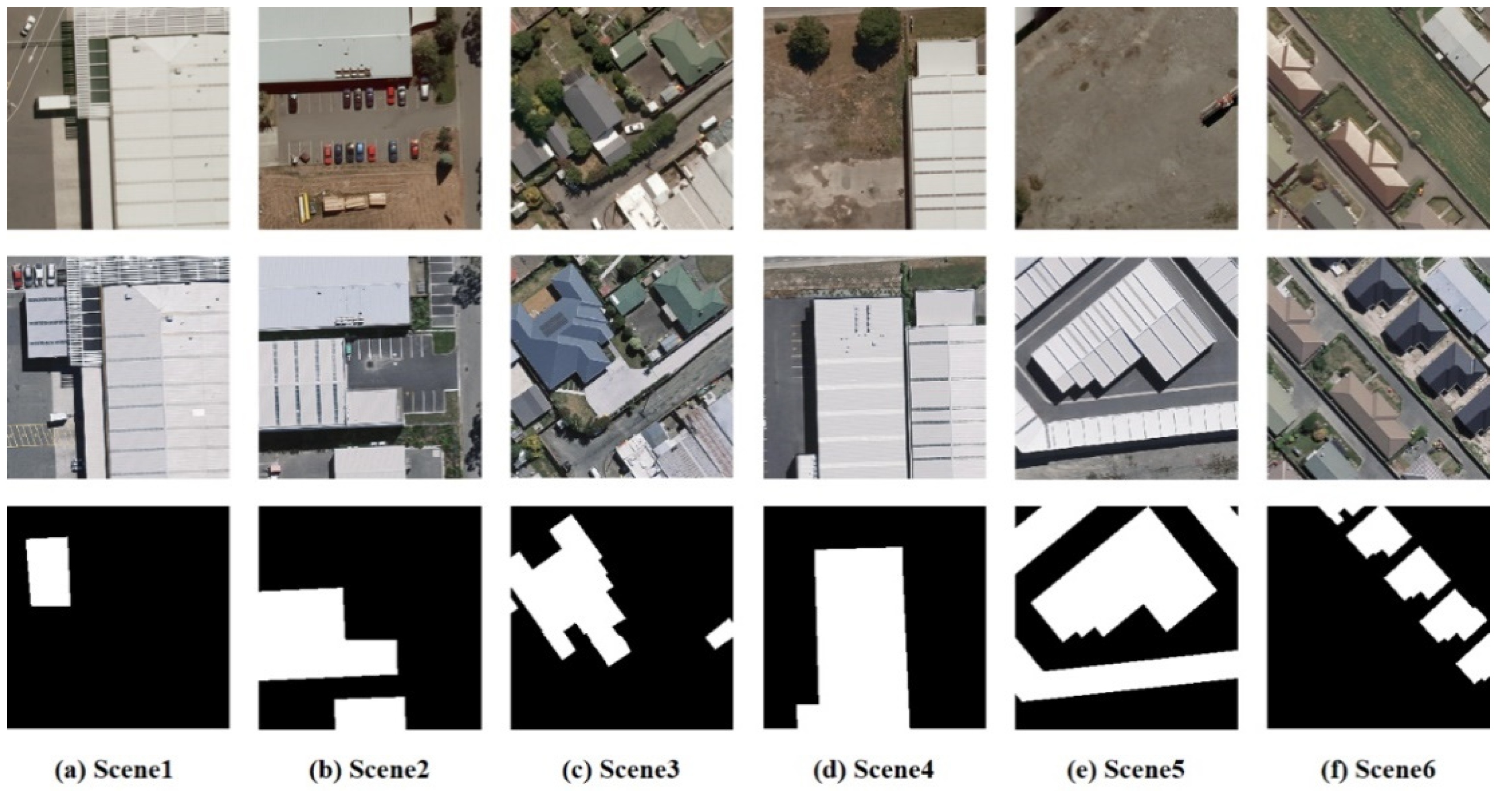
Figure 3, a few scenes are taken from the LEVIR-CD dataset.
Sun Yat-Sen University created the challenging SYSU-CD dataset [
41] for CD. This dataset contains changes in vegetation and buildings in a forest, buildings along a coastline, and the appearance and disappearance of ships in an ocean. The image size is 256 × 256 pixels with a resolution of 0.5 m. In our work, the training, validation, and test sample proportion was 6:2:2. Therefore, we obtained 12,000, 4000, 4000 pairs of patches for training, validation, and testing, respectively.
Figure 4 illustrates some of the variety of the scenarios included in the SYSU-CD dataset.
The WHU-CD dataset [
42] was released by the University of Wuhan as a public CD dataset. Only one image is included in the original dataset, which is 15,354 × 32,507 pixels. In order to be consistent with the two datasets mentioned above, 7432 patches were generated by cropping the image into 256 × 256 pixels. During the splitting, no overlap was used. In the end, we obtained 5201, 744, and 1487 pairs of patches for the training, validation, and testing, respectively. A few scenes from the WHU-CD building dataset are shown in
Figure 5.
3.2. Experimental Details
3.2.1. Evaluation Metrics
Remote sensing CD presents a problem regarding the binary classification of the pixels. CD algorithms are therefore evaluated using the following quantitative evaluation metrics that are commonly used in binary classification problems: precision (P), recall (R), F1 score, mean intersection over union (mIOU), overall accuracy (OA), and kappa coefficient. Precision indicates fewer false detections, while recall indicates fewer missed detections. The higher the mIOU and F1 scores, the better the performance. We also added two additional values, where IOU_0 and IOU_1 indicate that an unchanged or changed region is detected, respectively. The OA provides an overall assessment of the model’s performance, with higher values representing a better performance. The consistency is checked using the kappa coefficient. Specifically, we defined the evaluation metrics as follows:
In the above formulas, true positive is abbreviated as TP. False positive is referred to as FP. True negative is abbreviated as TN. False negative is referred to as FN.
3.2.2. Parameter Settings
Throughout the experiments, we employed the PyTorch framework to build all the models. We used NVIDIA GeForce RTX 3090 GPU in our experiments. Based on the limitations of the GPU memory, we set the batch training size to eight when configuring the parameters of the network model training. The maximum number of epochs we used for training the model was 200. Training was stopped early during the process in order to prevent overfitting. Our initial learning rate was 0.0002. In the overall training process, the model with the highest performance on the validation set will be applied to the test set for testing.
3.3. Ablation Experiment
In order to confirm the effectiveness of our proposed SCA and DCD modules, we conducted ablation experiments using the LEVIR-CD dataset, and the results are shown in
Table 2.
The F1 score increased from 89.48% in the baseline to 89.81% when the SCA module was added separately. As a result of the simultaneous addition of the SCA and DCD modules, the model’s F1 score increased by 0.84% over the baseline, reaching 90.32%. With just the SCA module, the precision improved by only 0.64%, but with the additional use of the DCD module, the precision improved by 2.41%, demonstrating that the DCD module is effective at reducing missed detections. Finally, when all the modules were applied to the baseline, the precision and IOU_1 for the CD reached their highest values of 90.14% and 83.37%, respectively. These values are significantly higher than the baseline.
3.4. Comparative Experiments
We selected several classical CD models as well as the existing SOTA models for comparison experiments to demonstrate the accuracy and effectiveness of SCADNet. The selected algorithms are described in detail as follows:
FC-EF [
43]: A method of image-level fusion in which bitemporal images are concatenated to shift the single input to a fully convolutional network, and feature mapping is performed through skip connections.
FC-Siam-conc [
43]: This method fuses the multiscale information in the decoder. A Siamese FCN is employed, which uses the same structure and shared weights to extract multilevel features.
FC-Siam-diff [
43]: Only the skip connection is different between this method and FC-Siam-conc. Instead of concatenating the absolute values, FC-Siam-diff uses absolute value differences.
CDNet [
44]: CDNet is initially used to detect street changes. The core part of the network is four compression blocks and four extension blocks. The compression blocks acquire feature information about the images and the extension blocks refine the change regions. Softmax is used to classify each pixel point for the prediction, balancing performance, and model size.
IFNet [
45]: An image fusion network for CD that is deeply supervised. The bitemporal images are first extracted using a two-stream network. The feature information is then transferred to the deep supervised difference discrimination network (DDN) for analysis. Finally, channel attention and spatial attention are applied to fuse the two-stream feature information to ensure the integrity of the change region boundaries.
SNUNet [
46]: SNUNet reduces the loss of deep information in neural networks by combining the Siamese network and NestedUNet. In addition, an ensemble channel attention module (ECAM) is used to achieve an accurate feature extraction.
BITNet [
47]: A transformer module is added to the Siamese network to transform each image into a set of semantic tokens. This is followed by building a contextual model of this set of semantic tokens using an encoder. Finally, a decoder restores the original information of the image through a decoder, thus enhancing the feature representation in the pixel space.
LUNet [
48]: LUNet is implemented by incorporating an LSTM neural network based on UNet. It adds an integrated LSTM before each encoding process, which makes the network operation more lightweight by adjusting the weight of each LSTM, the bias, and the switch of the forgetting gate, thus achieving an end-to-end network structure.
We employed a total of twelve methods to conduct comparative experiments; we do not have an open source well reproducible code for the four methods (DeepLabV3, UNet++, STANet, and HDANet) [
49]. Therefore, to respect the existing work, we directly referenced the available accuracy evaluation metrics on the BCD datasets.
Table 3 shows the comparison results of the various methods on the LEVIR-CD dataset. SCADNet outperformed other networks in all the metrics except precision. The F1 score and recall metrics also showed an excellent performance (90.32% and 91.74%, respectively). HDANet achieved the highest precision of 92.26%, which was 2.12% better than our method. Since SCADNet is focused not only on correctly detecting the areas that are really changing, but also on all areas where a change occurs. The recall metric of our method was higher than HDANet’s of 4.13%. In light of the F1 score metric, we can conclude that our method had the most robust overall performance.
We selected two scenarios from each of the three BCD datasets for visualization. As can be seen in
Figure 6, there is only one variation in the building. Due to the changes in lighting, all the methods except SNUNet and SCADNet detected the house in the lower-right corner as a building change. In addition, we achieved fewer false detections compared with SNUNet in the upper-left corner of the building.
As shown in
Figure 7, our method was able to detect a dense multi-objective building change scene with a total of three rows of buildings changing. In contrast, all the other methods failed to detect the relatively small changes in the second row of the buildings. While FC-EF, FC-Siam-conc, and FC-Siam-diff almost completely missed these small targets, our method was successful in identifying them. In addition, SCADNet was also able to achieve a low false detection rate for slightly larger buildings.
Table 4 shows the comparison results for the SYSU-CD dataset. Our method achieved optimal results in terms of the F1 score, mIOU, IOU_0, IOU_1, OA, and kappa metrics. One of the most notable results was our F1 score of 81.79%. Among the other methods, the F1 score of the IFNet also reached 80.98%, which is only 0.81% lower than that of our method, while the SCADNet was second only to UNet++, DeepLabV3, BITNet, and STANet in terms of the precision. With the multi-scale feature fusion strategy, IFNet exhibited the highest recall rate of all the methods, reaching 87.60%. DeepLabV3 and the three FC-based methods had a relatively insufficient detection accuracy. For example, the F1 score and precision for FC-EF were 75.13% and 64.58%, respectively, which were 6.66% and 15.54% lower than those for our method.
Figure 8 shows a scene from the SYSU-CD dataset, where only a small portion of the upper part of the image has building changes and the site environment is complex. Aside from the SCADNet, FC-EF, CDNet, and IFNet, all the other methods misidentified vegetation changes as building changes. Further, the CDNet performed second only to the SCADNet and caused only a few false detections around the change area. Even though the SCADNet did not completely detect the actual change area, it was able to avoid the occurrence of false detections.
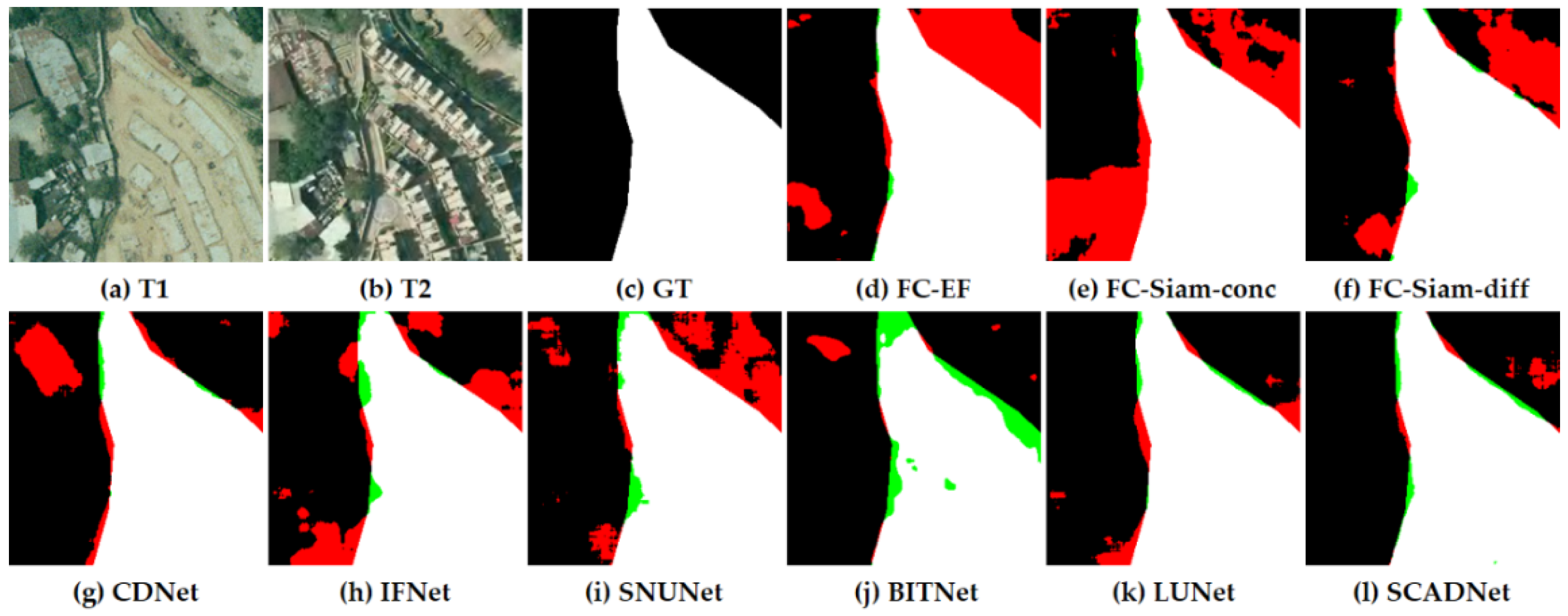
There are large-scale building changes in
Figure 9. In spite of the fact that all the methods were able to detect the main part of the changed building, they did not perform the BCD effectively. Among them, the BITNet missed a significant part of the changed area, while other methods except the LUNet and SCADNet had a large area of false detection. Furthermore, the SCADNet detected edges more accurately when it came to identifying the changed regions.
The metrics for each method are compared in
Table 5 on the WHU-CD dataset. Our method was still able to outperform the other methods in terms of the F1 score, mIOU, IOU_0, IOU_1, OA, and kappa metrics. Although FC-Siam-diff achieved 94.30% in recall, outperforming our method by 1.8%, its precision only reached 65.98%, which is 19.08% lower than ours. Similarly, the HDANet achieved an optimum precision of 89.87%, which was 4.81% higher than our method, but its recall was 9.55% lower than that of the SCADNet. Moreover, our method achieved an F1 score value of 88.62%, indicating that it has a better comprehensive BCD performance.
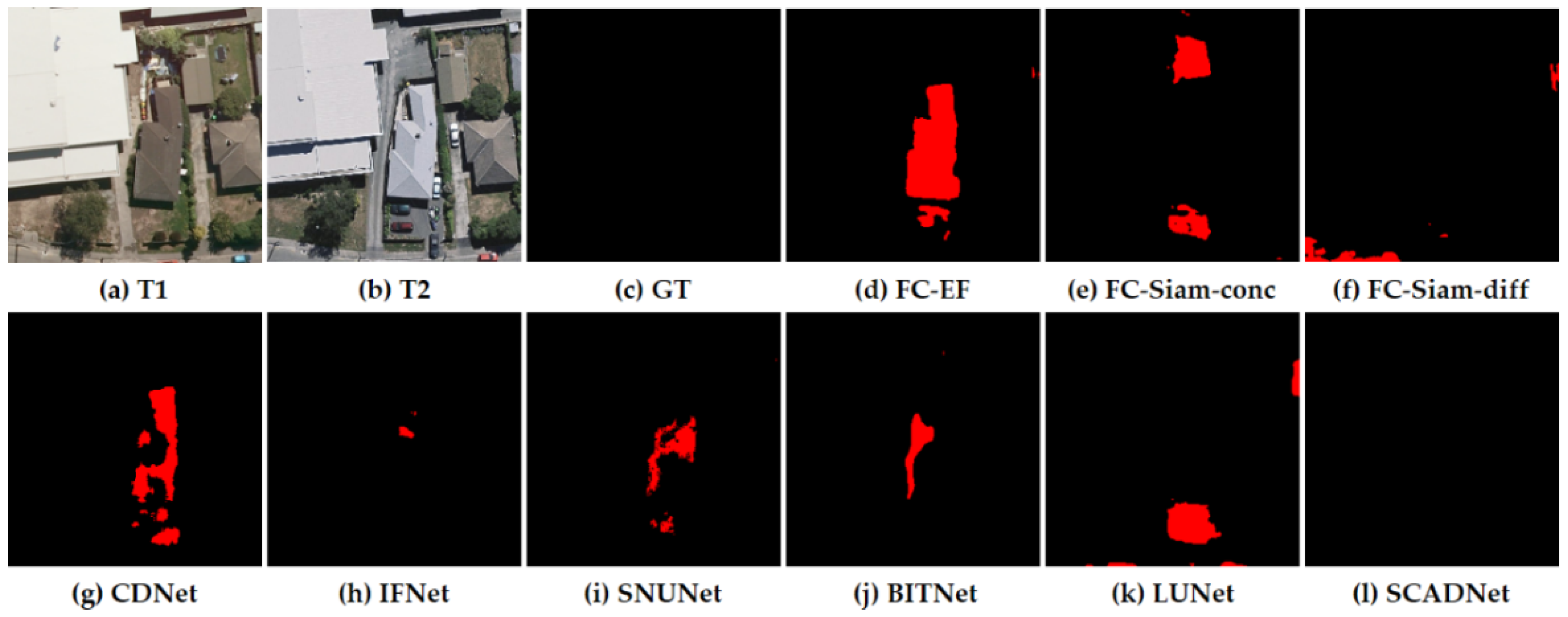
Figure 10 shows that there is no change in the building, and the change in the roof color of the building caused all the other methods to produce false detections. The FC-EF, CDNet, and SNUNet all identified the area where the building already exists as the change area, while the BITNet and LUNet classified the road change as a building change. Our method did not cause any false detections or omissions, and the detection results were consistent with GT, achieving optimal results.
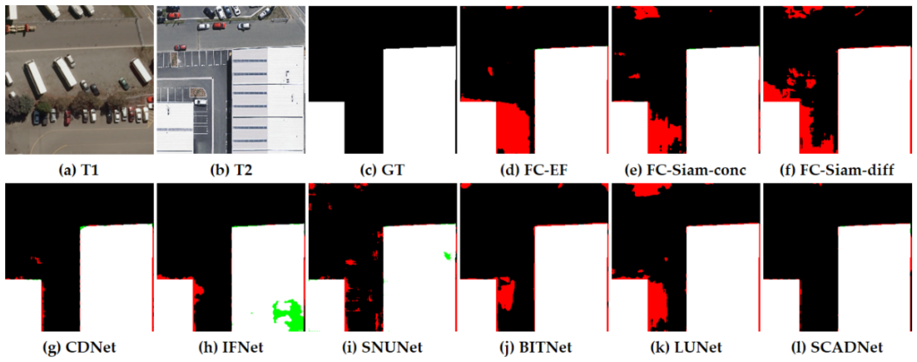
The T1 and T2 images in
Figure 11 have changed drastically, but there are only two building changes, one of which is a large building change. All the methods were able to detect these two building change areas; however, the FC-EF, FC-Siam-conc, FC-Siam-diff, BITNet, and LUNet all incorrectly identified the parking space as a changed building. Moreover, the IFNet missed part of the change area, while our SCADNet completed the BCD to near perfection.
3.5. Quantitative Results
We selected 100 images from the LEVIR-CD dataset for a quantitative evaluation and comparison.
Figure 12 shows the comparison of various methods across eight metrics.
The SCADNet presented a remarkable superiority in terms of the F1 score, mIOU, IOU_0, IOU_1, OA, and kappa metrics. As far as the F1 score is concerned, our method was significantly better than the others. The SCADNet also achieved relatively positive results for the precision metric (on par with SNUNet). Finally, the LUNet outperformed the SCADNet by only a slim margin in the recall metric.
3.6. Computational Efficiency Experiment
We employed two metrics, the number of parameters (Params) and floating points of the operations (FLOPs) to further compare the efficiency of the model of the eight comparative methods; note that the smaller the number of model’s Params and FLOPs, the lower the model’s complexity and computational cost. For each method, we gave two images of size 1 × 3 × 256 × 256 as the inputs, and the computational efficiency results are shown in
Table 6. Because of the simple network architecture, the Params and FLOPS values for the FC-based method and CDNet were relatively low. Due to the deep layer of the networks and the multi-scale feature fusion strategy, both the IFNet and SCADNet generated a large number of Params, but our FLOPs were still lower than IFNet.
4. Discussion
Based on three public BCD datasets, the SCADNet was comprehensively evaluated. The SCADNet was further evaluated quantitatively and qualitatively against several popular methods to demonstrate its superiority. This is mainly due to the following three aspects: first, the conventional methods focus primarily on the changed regions of the bitemporal images. As a result, if the background of the bitemporal images changes significantly, it will cause a large area of false detection. Our SCA module is able to differentiate the changed and the unchanged regions in the bitemporal images and extracts the actual changed feature information accurately for an improved BCD performance. Second, due to the different number of channels and the degree of representation, the multi-scale feature information extracted by direct fusion will result in the redundancy of unimportant information and the loss of key information. To reduce the error detection rates, the MFF module gradually integrates the multi-scale feature information with rich semantic information and recovers the original feature information of the image to the maximum extent possible. Third, in contrast to the traditional method of directly generating BCD results, our DCD module can jointly consider the predicted image and the difference image to calculate the probability loss. This allows us to provide a more detailed analysis of the building changes, thus reducing the missed detection rates.
Furthermore, we will analyze our SCA module by visualizing the attention maps. For the BCD, it is imperative to identify not only the changed buildings but also the unchanged environments. As a Siamese neural network consists of multiple layers, the downsampling results in the loss of local details. The abundant detail information in the image can be perceived by adding an attention mechanism, thus alleviating the above problem. In addition, the cross-attention mechanism can also effectively focus on the similarities and differences between the pixel points in the bitemporal images, enhancing the neural network’s attention to tiny buildings in the images, reducing the noise by correlating the bitemporal images, clarifying the edges of the changes, and completing the CD by connecting the two streams of cross-attention information. As shown in
Figure 13, we provide several examples of how our method visualizes attention maps at different stages of the SCADNet. Blue indicates lower attention values, while red indicates higher attention values.
We performed the attention map visualization operations on all three of our datasets and took two images from each dataset as a display. There are two parts to our cross-attention mechanism, invariant attention, and changing attention channels.
There are a number of changes in dense, tiny buildings in the first image of the LEVIR-CD dataset, and our attention channels focus on the environmental information that has not changed in the before and after time series, as well as the regions where there are buildings changes. In Stage 1, the change attention channel only detects a small portion of the changed buildings, and the color is not particularly red; however, as the network layers deepen, our change attention channel gradually becomes more focused on the changed areas. Until Stage 4, our changing attention channel peaks for the changed region and shows a dark blue color for the content of the unchanged region. At the same time, the invariant attention channel also reaches its maximum attention in the unchanged regions. In the second scene of LEVIR-CD, the attention module does not only focus on changes in large buildings in the middle region, but also on changes in buildings on the left all the time.
For the SYSU-CD dataset, with an increasing number of network layers, the invariant attention channel focuses more on non-building change information, such as the ocean and vegetation, etc. The changing attention channel focuses on ship information in the first picture and the emerging buildings on both sides of the mountain in the second picture.
As part of the WHU-CD dataset, we also collected two scenarios, which show regular building changes. Our two-channel attention is still able to better distinguish between unchanged and changed regions, especially in the second scenario, where the invariant attention channel concentrates most of its attention on the unchanged regions, whereas the changing attention channel focuses only on regions where building changes occur.
According to the visualization results, our network’s attention mechanism module efficiently captures the high-level semantic information needed for BCD, and this high-level semantic information serves as strong data support. Using two-channel attention, the SCADNet is capable of focusing on its own region of interest, resulting in a superior accuracy.
5. Conclusions
A novel BCD method called the SCADNet was proposed in our study. An SCA module was used to identify the changed and unchanged regions in the bitemporal images. An MFF module was proposed in order to fuse the multi-scale feature information and reduce the key information loss during the feature map fusion process. To distinguish whether the change information in the extracted feature maps is a pseudo-change, we applied the DCD module to filter out the regions where real changes occur. The experimental results demonstrate that the SCADNet is superior to other methods using the LEVIR-CD, SYSU-CD, and WHU-CD datasets. The F1 score on the three datasets above can reach 90.32%, 81.79%, and 88.62%, respectively.
In this study, we conducted experiments on only three datasets, which do not effectively represent the generalization of the SCADNet, and subsequent experiments can be conducted on more remote sensing image CD datasets.
The combination of CD and semantic segmentation will be further investigated in the future. Additionally, the proposed method is based on an extensive collection of annotated samples, which is essential for supervised learning, in order to reduce the dependence of the CD methods on high-quality datasets. Therefore, we intend to conduct future research using a combination of the unsupervised methods and CD.


 ,
, 


