Article

Optimization Method of Airborne LiDAR Individual Tree Segmentation Based on Gaussian Mixture Model

1
College of Geodesy and Geomatics, Shandong University of Science and Technology, Qingdao 266590, China
2
Department of Geomatics Engineering, Schulich School of Engineering, University of Calgary, 2500 University Drive NW, Calgary, AB T2N 1N4, Canada
3
Lyles School of Civil Engineering, Purdue University, West Lafayette, IN 47907, USA
*
Author to whom correspondence should be addressed.
Remote Sens. 2022, 14(23), 6167; https://doi.org/10.3390/rs14236167
Submission received: 26 September 2022 / Revised: 29 November 2022 / Accepted: 2 December 2022 / Published: 5 December 2022
(This article belongs to the Special Issue 3D Point Clouds in Forest Remote Sensing II)

Abstract

:
Forests are the main part of the terrestrial ecosystem. Airborne LiDAR is fast, comprehensive, penetrating, and contactless and can depict 3D canopy information with a high efficiency and accuracy. Therefore, it plays an important role in forest ecological protection, tree species recognition, carbon sink calculation, etc. Accurate recognition of individual trees in forests is a key step to various application. In real practice, however, the accuracy of individual tree segmentation (ITS) is often compromised by under-segmentation due to the diverse species, obstruction and understory trees typical of a high-density multistoried mixed forest area. Therefore, this paper proposes an ITS optimization method based on Gaussian mixture model for airborne LiDAR data. First, the mean shift (MS) algorithm is used for the initial ITS of the pre-processed airborne LiDAR data. Next, under-segmented samples are extracted by integrated learning, normally segmented samples are classified by morphological approximation, and the approximate distribution uncertainty of the normal samples is described with a covariance matrix. Finally, the class composition among the under-segmented samples is determined, and the under-segmented samples are re-segmented using Gaussian mixture model (GMM) clustering, in light of the optimal covariance matrix of the corresponding categories. Experiments with two datasets, Trento and Qingdao, resulted in ITS recall of 94% and 96%, accuracy of 82% and 91%, and F-scores of 0.87 and 0.93. Compared with the MS algorithm, our method is more accurate and less likely to under-segment individual trees in many cases. It can provide data support for the management and conservation of high-density multistoried mixed forest areas.

1. Introduction

Forests are an indispensable resource and environment for human survival and development. Forests play an irreplaceable role in biodiversity conservation, carbon sinks, water storage, and energy reserves, as well as maintaining the ecological balance of the planet [1,2,3]. How to protect and manage forest resources is an important issue for sustainable human development [4,5].
Airborne LiDAR can efficiently acquire high accuracy, large range 3D information on surface features with high levels of mechanization and automation [6,7,8]. Because it can effectively record the vertical structure characteristics of forests and extract canopy structure parameters [9,10,11], it shows great potential in the fields of forest conservation and management, ecological research, and carbon sink calculation [12]. Extracting high accuracy individual tree point cloud information from massive point cloud data makes it possible to calculate the structural parameters of individual trees (tree height, diameter at breast height, crown width, etc.) [13]. It also lays the groundwork for the subsequent biomass inversion [14,15] and 3D model construction of forests.
To further improve ITS accuracy, some methods choose to enhance the depiction of canopy boundaries, such as using the detailed vertical structure of the canopy in high-density LiDAR to improve information acquisition for individual canopies [16] and using marker-controlled watersheds to effectively control the detection of canopy boundaries [17,18]. There are also some methods to improve the local maximum detection algorithm, such as unfolding the local maximum (LM) algorithm from multiple scales to improve the accuracy of LM obtained by CHM at different spatial resolutions [19]; detecting individual tree height extremes by clustering the centers of cluster height points (CCHP) [20]; or using variable windows (VW) to avoid extremes of smaller canopies being ignored by larger fixed windows [21]. Moreover, a large number of computer vision theories have been applied to CHM methods. For example, the spike-free digital surface model [22], double Gaussian filter [23], and deep convolutional network [24]. CHM-based treetop detection techniques when used singlehandedly can detect and delineate most of the dominant crowns, but often fail to detect subdominant tree crowns.
CHM-based segmentation algorithms are usually suitable for coniferous forests with clear crown patterns and well-defined boundaries or forests with low canopy density. For broad-leaved forests with high canopy density, missed segmentation or wrong segmentation can often arise as a result of canopy obstruction. Compared with CHM-based segmentation methods, the direct use of point cloud data for ITS can make more use of the 3D structural information of the forest. It can recognize more understory trees, thus ensuring a higher accuracy of individual tree recognition and individual tree factor extraction [25,26].
Point cloud-based ITS methods focus more on the spatial structure of individual trees rather than on the boundary description of the canopy. For example, bottom-up segmentation methods based on vertical structural features of trees exploit the spatially separable differences between trunk and canopy layers [27,28]. In addition, based on spatial clustering features, point clouds, voxels [29], or super voxels [30,31] are used as processing units to perform ITS by clustering algorithms such as K-means or Mean Shift [32,33] or to optimize segmentation results with the distance minimization principle. Meanwhile, due to the limited information of pure spatial point clouds, some studies have used information gained from statistical methods, for example, generating height maps from airborne LiDAR data based on generative adversarial networks and performing ITS by Yolo-v4 [34]; or using spatial-spectral domain fusion to refine the segmentation by enhancing the description of the forest component structure with multispectral information to compensate for the monochromatic wavelengths in laser point clouds deficiencies [35]. These point cloud-based algorithms describe independent tree structures at the 3D level, allowing for better detection of trees in the understory as well as effective separation of overlapping tree populations.
All these methods have achieved good results in the experimental areas, but they did not perform so well on forests with high canopy density and mixed forests with complex tree species. The accuracy of segmentation is often compromised by over- or under-segmentation due to overlapping, obstruction, and excessive shape difference of canopies that cause incomplete segmentation or misclassification of individual trees. Furthermore, as existing ITS methods rarely consider the integrity of the segmented canopy, they can hardly ensure the accuracy of the individual segmented tree canopy. In view of these under-segmentation problems, this paper proposes an ITS method based on the Gaussian Mixture Model (GMM) clustering as an addition to the MS algorithm. The experimental results show that, compared with the MS algorithm alone, for high-density, multistoried mixed forests, our method has a higher ITD rate and is better able to describe canopy details. It can effectively reduce under-segmentation caused by the overlapping, obstruction, and excessive shape difference of canopies.

2. Materials and Methods

2.1. Study Area

There were two experimental areas. One of the experimental areas was in the forest northwest of Trento, in the province of Trento, Italy, at latitude 46°18′N and longitude 10°46′E. Another experimental center was located in the south of Qingdao, Shandong Province, China, Shandong University of Science and Technology campus of artificial forest, at latitude 35°59′N and longitude 120°07′E.
Trento’s experimental area covers an area of about 3.9 hectares, as shown in Figure 1a. The overall topography is relatively steep, with vertical drops of up to 60 m. The area is subject to westerly winds and prevailing oceanic air masses. The climate is mild and humid, with a small temperature difference, little rainfall, and low soil water content. The average tree height in the study area is 32 m with a stand density index of 974. The main tree species are larch, spruce, fir, sycamore, and poplar. Coniferous forest vegetation accounts for 80%. Forests there are mostly multistoried mixed forests.
The experimental area of Qingdao covers an area of about 1.8 hectares, and the overall terrain is relatively flat, as shown in Figure 1b. It has both a monsoon climate and marine climate characteristics. The air is humid, the precipitation is moderate, the rain and heat are in the same season, and the soil moisture content is moderate. There are many tree species in the area, including magnolia, black oak, money pine, maple, etc., and the coniferous forest content is about 45%, which is also a multi-layered mixed forest.

2.2. Dataset

Trento’s experimental data came from the ITD benchmark dataset provided by the open source website NEWFOR [36]. The scanner model used was RieglLMS-Q680i. The point density of the dataset was approximately 121 pts m−2. The minimum sampling density of the initial echoes was set to 10 pts m−2. At least four echoes were captured per signal. The airborne LiDAR data were georeferenced using the coordinate system UTM-32N (EPSG: 32632). The Qingdao experimental data were captured by the AP-0300 airborne LiDAR instrument, for which the sensor wavelength was 1550 nm, and the echo mode was multiple echoes. When the aircraft was flying, the relative altitude was 261 m, the absolute altitude was 263 m, the flight speed was 70–80 km/h, the heading overlap rate was 85%, and the side-facing overlap rate was 75%.
As the point density of the Trento dataset was too high and the stand density was large, the entire dataset was first down sampled with a voxel size of 0.35 in order to reduce computation and improve efficiency. Next, we divided the experimental plots based on a roughly equal area. Six experimental sample plots with an approximate area were divided from the Trento dataset and named Plot_d1-Plot_d6. The Qingdao experimental area was smaller, and stand density was lower, so four experimental plots with a similar area were isolated from the Qingdao dataset and named Plot_s1-Plot_s4. Information on the number of trees, tree height, crown width, and crown area in the ten experimental sample plots was obtained through the open source software Cloud Compare, as shown in Table 1. Since Trento’s data stand density was higher and Qingdao’s was lower, the Trento dataset was used as a complex stand and the Qingdao dataset was used as a simple stand for the comparative experiment.

2.3. Overview of the Proposed Methodology

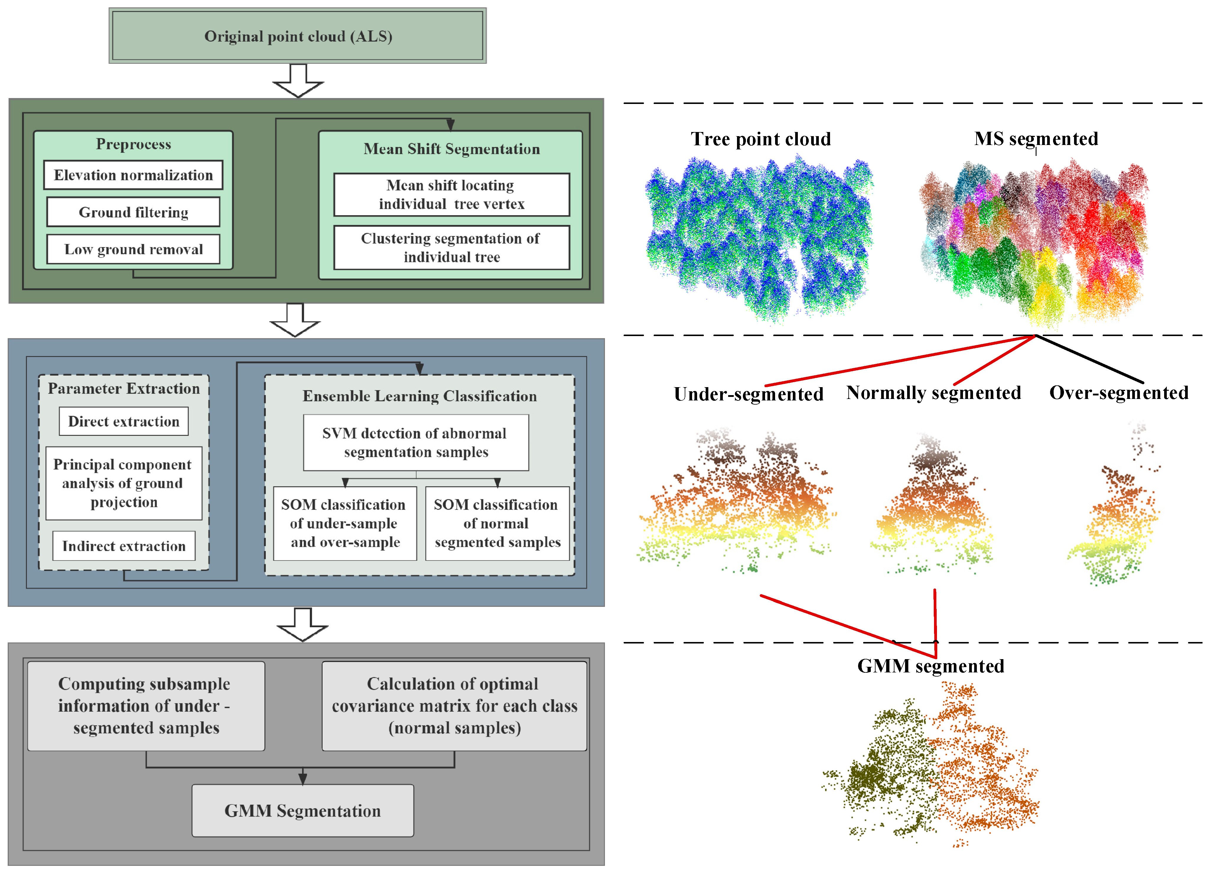
The new algorithm implements the following steps: first, MS is used to segment individual trees; next, under-segmented and normally segmented samples are picked out from the segmentation result by serial integrated learning, the canopy morphological parameters are used as the input features, and the normally segmented samples are classified by morphological approximation; the optimal covariance matrix for each type of the normally segmented samples is calculated, the point cloud distribution probability density of the under-segmented samples is described by GMM, and the segmentation of the under-segmented samples is optimized by clustering different types of samples according to their respective optimal covariance matrices. The flowchart of the overall algorithm is shown in Figure 2.

2.4. Pre-Processing

The existence of ground points will make the experiment more difficult [37]. Therefore, before performing ITS based on MS, we pre-processed the experimental data. First, we smoothed the terrain by elevation normalization. Then, we filtered out the ground point clouds by the cloth simulation filter (CSF) algorithm. Finally, by setting the elevation threshold we removed the features below the elevation threshold as low vegetation and obtained the canopy point cloud of the experimental plot. The elevation threshold of Trento dataset was 2.5 m, while Qingdao dataset was 2.0 m.

2.5. ITS Based on MS

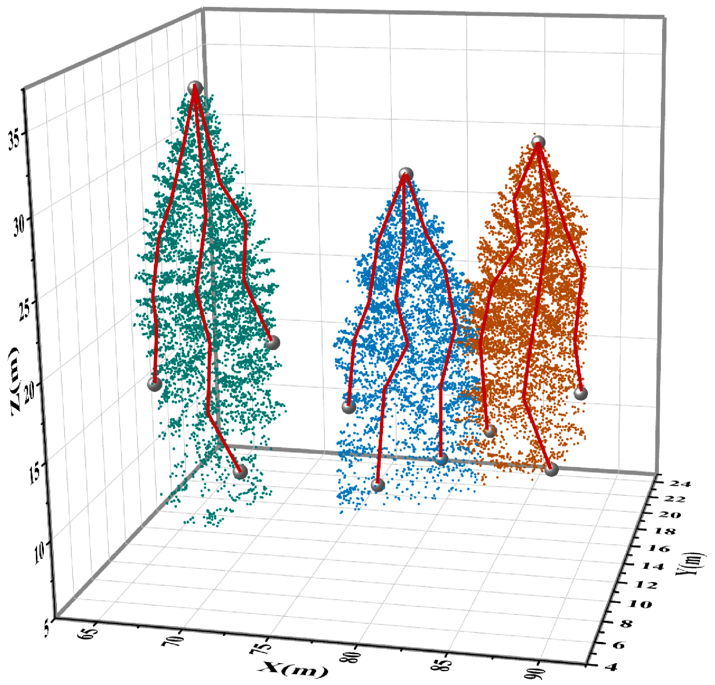
MS is a nonparametric eigenspace analysis technique, an algorithm used to locate local maxima of the probability density function of a data sample, so that the mean shift vector always points in the direction of the maximum increase in the density of the data parameters [38]. This concept was first proposed by Fukunage et al. and was improved and extended by Cheng et al., who defined the kernel function and added a weight coefficient [39,40]. The MS algorithm has a wide range of applications in clustering, image smoothing, segmentation, and video tracking. The principle is as follows: the mean shift clustering segmentation iterates continuously from the initial seed point and moves with the mean shift vector. When the seed point no longer moves or the distance is shorter than the set threshold, it is considered to have reached a local maximum of density. In ITS, the seed point gradually moves towards the vertex of the individual tree canopy (where the point cloud density is the greatest), as shown in Figure 3. Points within the final position bandwidth are grouped into a cluster. Those aggregated to the same cluster are grouped into another.
As mentioned earlier, it has been shown through kernel functions that the contribution of each point to the mean shift vector in the high-dimensional spherical region varies with the distance from the point to the center point. To find the maximum value of the probability density function, one would directly turn to taking its derivative, and then obtaining the formula of the mean shift vector from the derivative equation.
However, with real use of 3D point cloud data, placing all the points in the same direction with the same regular weight ratio is also not well suited for application. Therefore, the actually used algorithm operates by dividing the 3D space into horizontal and vertical domains [41,42]. The offset of the seed point for each iteration is calculated by Equation (1):
m h s , h r ( X ¯ ) = i = 1 n X i g s | | X ¯ s X i s h s | | 2 g r | | X ¯ r X i r h r | | 2 i = 1 n g s | | X ¯ s X i s h s | | 2 g r | | X ¯ r X i r h r | | 2 X ¯
where gs and gr are the two correlation kernel functions used to search for local density maxima in the horizontal domain and local height maxima in the vertical domain, respectively. hs and hr are the bandwidths of the horizontal and vertical domains. In addition, Xi = (xi, yi, zi), Xis = (xi, yi), Xir = (zi). As the appropriate degree of bandwidth often determines the effect of the MS algorithm for ITS, it is often necessary to adjust the bandwidth according to the conditions of the experimental plot. In the experiments, the horizontal bandwidth hs and vertical bandwidth hr used for MS segmentation of the Trento dataset were 1.5 m and 5.0 m, respectively, while the hs and hr of the Qingdao dataset were 1.0 m and 2.5 m, respectively.

2.6. Optimal Covariance Matrix Calculation

2.6.1. Parameter Extraction and Sample Classification

After the forest point cloud of the plot is divided by MS, a number of individual trees point cloud samples can be obtained. First, the 3D point cloud data of each individual tree sample is mapped from Euclidean space to a thirteen-dimensional Hilbert space in a certain way by means of spatial transformation to obtain the thirteen-dimensional feature parameters of each sample, so that all samples are placed in the same space and processed together. The names of the characteristic parameters and their descriptions are shown in Table 2.
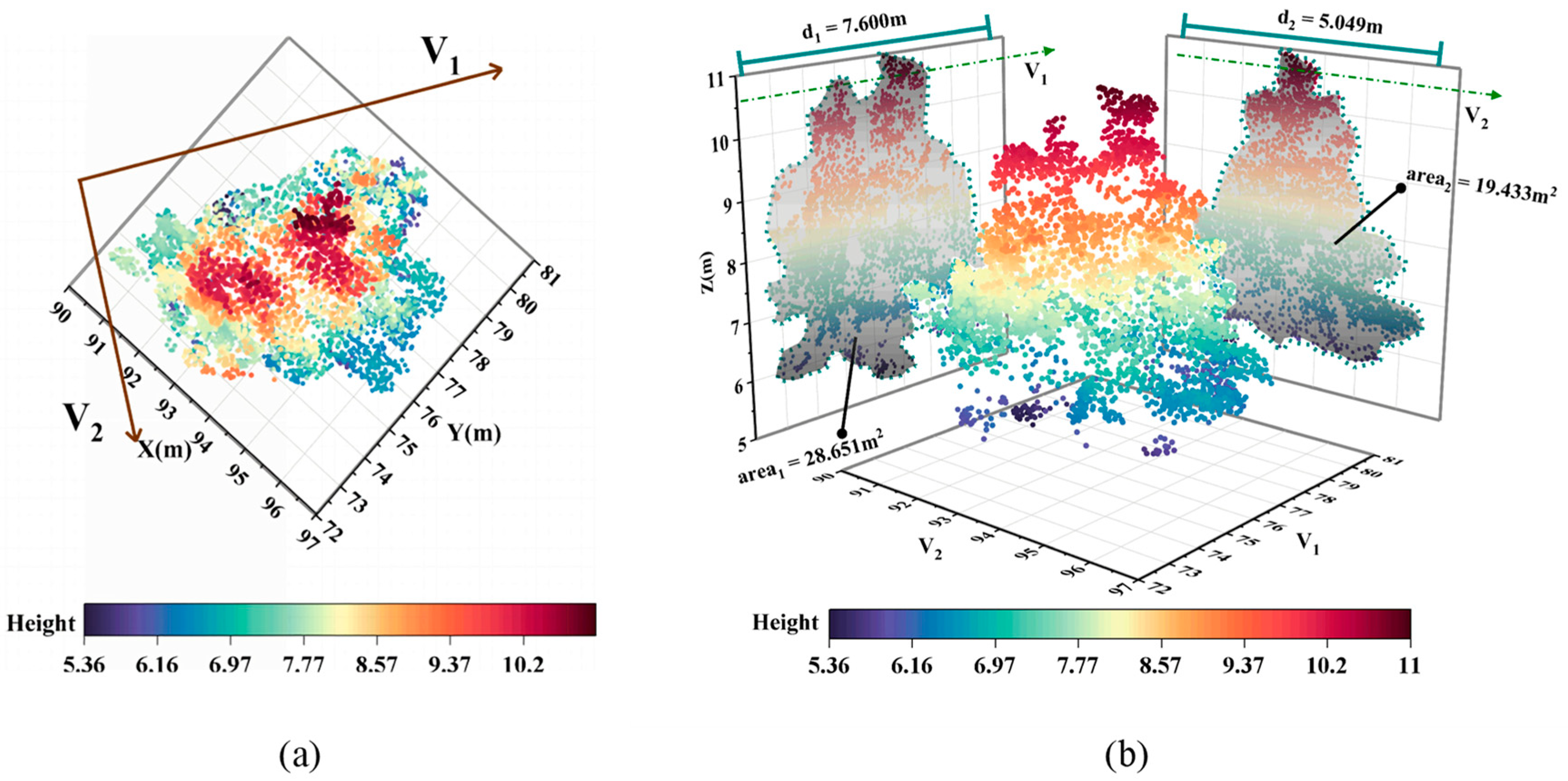
The first seven feature parameters can be extracted by directly calculating the 3D point cloud data. The last six feature parameters have to be extracted indirectly in the following way: first, the sample is projected vertically to the horizontal ground; a principal components analysis (PCA) is performed on the projected point set to calculate the two orthogonal directions V1 and V2 with the longest canopy and the maximum information, namely, the principal canopy directions; then new axes are established based on these two directions, and the sample point clouds are projected onto the two vertical principal planes [35,43], as shown in Figure 4a.
After projecting the canopy point cloud to the two vertical principal planes, we can obtain two two-dimensional point sets {Pi1 | Pi1 = (xi, yi), i = 1, 2, 3, …,m} and {Pj2 | Pj2 = (xj, yj), j = 1, 2, 3, …,n}. The remaining six feature parameters can each be calculated from the point set. The longest distribution in the canopy direction is calculated by Equation (2). The longest distribution perpendicular to the canopy direction is calculated by Equation (3):
d 1 = x i max x i min
d 2 = x j max x j min
The ratio of the two is calculated by Equation (4):
d r = d 1 / d 2
After that, the alpha-shape is created for the two-projection point sets, respectively. The projection boundary is obtained based on the alpha-shape. area1 and area2 are calculated based on the boundary information. The ratio of the two is then calculated by Equation (5), thus completing the indirect extraction of the parameters:
a r e a r = a r e a 1 / a r e a 2
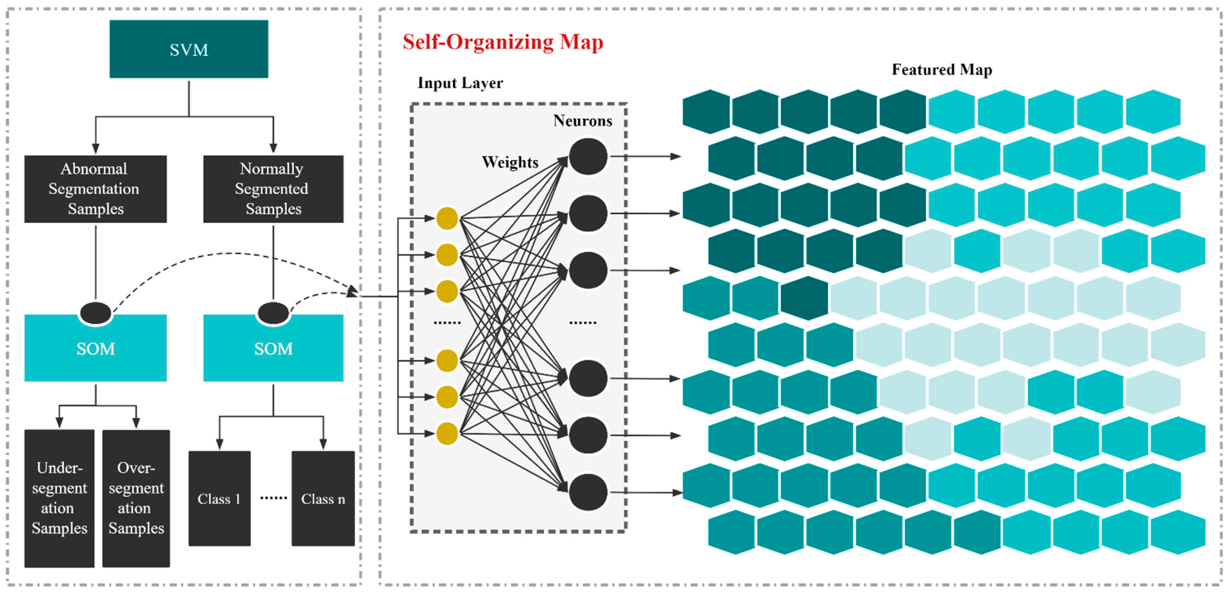
Once the feature parameters of all samples are extracted, the samples can each be represented by a thirteen-dimensional feature vector and then classified according to the flow shown in Figure 5. The classification of abnormally segmented and normally segmented samples is performed first. As binary classification based on a thirteen-dimensional feature vector is a matter of nonlinear classification in high-dimensional space, we first select some abnormally segmented and normally segmented samples from all samples, build training datasets with their parameters, build a binary classifier with the help of training support vector machines (SVM), and map the feature vectors of all samples to the point set in high-dimensional space to establish a delineation hyperplane. Based on the characteristics of the extracted parameter representations, all samples are classified into two categories: abnormally segmented and normally segmented.
After the total sample set is successfully divided into two subsets of abnormally segmented and normally segmented using SVM, the two subsets are then clustered based on the self-organizing map (SOM) neural network, respectively, since the feature vectors of the samples mainly describe their morphological features. SOM organizes the neurons in the neural network to compete with each other by inputting the feature vector of the sample, determining the adjacent samples in the input space against the relative distance as the metrics of approximation and approximating the topology of the input sample space by mapping it to the adjacent neurons. As shown in the featured map in Figure 5, each cell represents a neuron, and the number of cells represents the size of the mapping space. The same color means that they are closer together in the input space. For the abnormally segmented subsample set, under- and over-segmented samples can be separated by a constant iteration of SOM. For the normally segmented subsample set, the granularity and scale of the model is enhanced by adding the number of competing layer neurons to provide a larger two-dimensional mapping space. Based on the feature vectors of the samples, the network can perform a detailed classification based on morphological features to group the normally segmented subsample set into different classes based on morphological features.

2.6.2. Calculation of Optimal Covariance Matrix

After sorting out the under-segmented samples by SOM and grouping the normally segmented samples with similar morphology, assuming that each sample belongs to a ternary Gaussian distribution, the 3D coordinate point cloud in each sample can be regarded as the set of sample points in the distribution model to which each sample belongs {Xik | Xik = (xi, yi, zi), i = 1, 2, 3, …, n}. Maximum Likelihood Estimation (MLE) is used so that the prior probability model of the multivariate Gaussian distribution for the kth sample is written as in Equation (6):
P ( X | μ k , k ) = 1 ( 2 π ) 3 2 | k | 1 2 e 1 2 [ ( X μ k ) T 1 ( X μ k ) ]
Construct the log-likelihood function as shown in Equation (7):
L k ( P ) = arg max μ k , k ln k P ( X | μ κ , κ )
Take the partial derivatives of each parameter of the likelihood function Lk(P) and calculate the extreme value points to obtain the mean μk and covariance matrix ∑k of the distribution model to which each sample belongs.
Considering that the previous under-segmentation detection has some errors and the normally segmented samples based on morphological features also contain some extreme samples, if we want to calculate the optimal covariance matrix for similar samples, we need to inspect the abnormal samples in each class first. As a covariance matrix can describe the uncertainty of the distribution of all sample points, it can be used for abnormity inspection. First, the Frobenius norm is calculated for each sample covariance matrix. The Frobenius norm Fk of the covariance matrix ∑k for the kth sample in the sample set of each class is calculated by Equation (8):
F k = | | k | | F = i = 1 m j = 1 n | a i j | 2 = i = 1 min { m , n } σ i 2
where aij represents the elements in the matrix and σi represents the singular values of the matrix. The covariance matrix of each sample can be mapped from the vector space to the fugitive linear space using the above equation to obtain feature sets {Fknorm | Fknorm = Fk, k = 1, 2, 3, …, n}. Next, the mean and standard deviation STD.Deviation in the feature set are calculated, followed by the standard error STD.Error:
S T D . E r r o r = S T D . D e v i a t i o n n
This way a 95% confidence interval [Mean − 1.96 ∗ STD.Error, Mean + 1.96 × STD.Error] can be constructed. Using this confidence interval as the benchmark, if the Frobenius norm Fknorm of the kth sample is not within the interval, such as the sample corresponding to the red sample bar in Figure 6, it is considered abnormal and excluded.
When the abnormal samples are excluded, the median center of the covariance matrix of all remaining samples is calculated to obtain the optimal covariance matrix ∑best for that sample class. Using the average covariance matrix of all samples as the initial median center, the Frobenius norm of the difference matrix between the covariance matrix ∑k and the present median center of each sample is calculated as a measure of the degree of approximation between the two, as shown in Equation (10):
j + 1 m = k = 1 n k | | k j m | | F k = 1 n 1 | | k j m | | F , | | j + 1 m j m | | F > 10 6 j m , | | j + 1 m j m | | F < 10 6
where ∑jm is the present median center and ∑j+1m is the new median center obtained by the iteration. Through continuous iterative computation until the algorithm satisfies the convergence condition, the final median center is taken as the optimal covariance matrix ∑best for this sample class, which is the description matrix of the model of this sample class in terms of distribution uncertainty.

2.7. GMM-Optimized Segmentation

GMM clustering differs from other common clustering approaches in that, instead of explicitly delineating categories, it uses a probabilistic model to describe the clustering structure—it is a soft clustering approach. Given that the point cloud data of each individual tree sample itself does not satisfy the Gaussian distribution in any dimension, the individual tree samples separated by direct GMM clustering are not necessarily the optimal results that meet the expectations. Therefore, the distribution uncertainty described by the optimal covariance matrix ∑best for each sample class is used to guide the calculation of distribution models in GMM clustering. In the GMM model used to describe each under-segmented sample, the covariance matrix possessed by each sub-model makes it approximate the optimal covariance matrix for the class to which the subsample set belongs, namely, the similar distribution uncertainty, so that individual tree samples best meeting expectations are extracted from the under-segmented samples. The probability density function (PDF) of GMM for an under-segmented sample with a total of k mixed individual tree samples in a finite dimensional data space is shown in Equation (11):
P M ( X i ) = j = 1 k π j · P ( X i | μ j , j )
where πj represents the weight occupied by the jth sub-distribution model. Next, the expectation-maximizing algorithm (EM) is used to solve for the parameters. First, the log-likelihood function of the mixed model is constructed, as shown in Equation (12):
L L ( D ) = ln ( i = 1 n P M ( X i ) )
Based on the matrix variational derivative rule, the partial derivatives of each parameter are found for the polar solution to derive the mean value of each sub-distribution model as shown in Equation (13), the covariance matrix as shown in Equation (14), and the weights as shown in Equation (15):
μ j = i = 1 n γ i j X i i = 1 n γ i j
j = i = 1 n γ i j ( X i μ j ) ( X i μ j ) T i = 1 n γ i j
π j = 1 k i = 1 n γ i j
where γij represents the posterior probability of the ith sample point from the jth subdistribution model.
γ i j = π j P ( X i | μ j , j ) l = 1 k π l P ( X i | μ l , l )
By iterative computation we gradually approximate the optimal distribution with respect to the sample set until the convergence condition is reached.
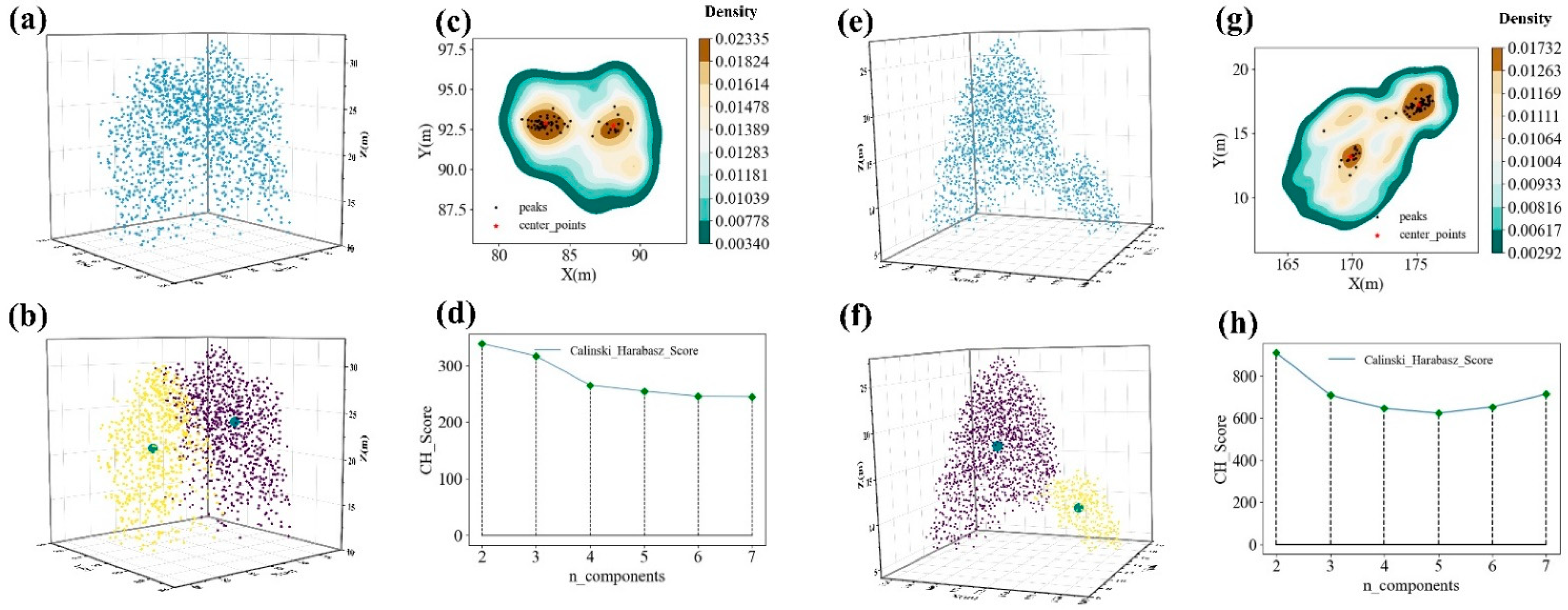
To obtain the number of subsamples in the under-segmented samples and their composition, first, a Gaussian kernel function is used to estimate the single-point kernel density for the set of projected points in the vertical ground direction for all sample points in each sample, as shown in Figure 7c,g. Next, peak point detection is performed to obtain a number of clusters consisting of high-density points. As for airborne LiDAR point cloud data, the higher the density, the closer to the top point, each cluster can be approximated as the top set of points of a subsample present in that under-segmented sample. Next, through repeated K-means clustering and by evaluating the inter-class variance and intra-class variance, the Calinski-Harbasz (CH) Score is obtained, and line plots of CH scores versus the number of clusters are plotted as in shown Figure 7d,h. A line graph clearly shows the optimal number of clusters [44,45], i.e., the number of subsamples present in this under-segmented sample.
Moreover, the mean value of each homogeneous group is approximated as the center point of each subsample, as shown by the green center points in Figure 7b,f. This way, we can determine the number of subsamples and detect the approximate center position of each of its subsamples regardless of whether the undivided samples are composed of canopies with approximate horizontal heights as shown in Figure 7a,b, or canopies with different horizontal heights as in shown Figure 7e,f.
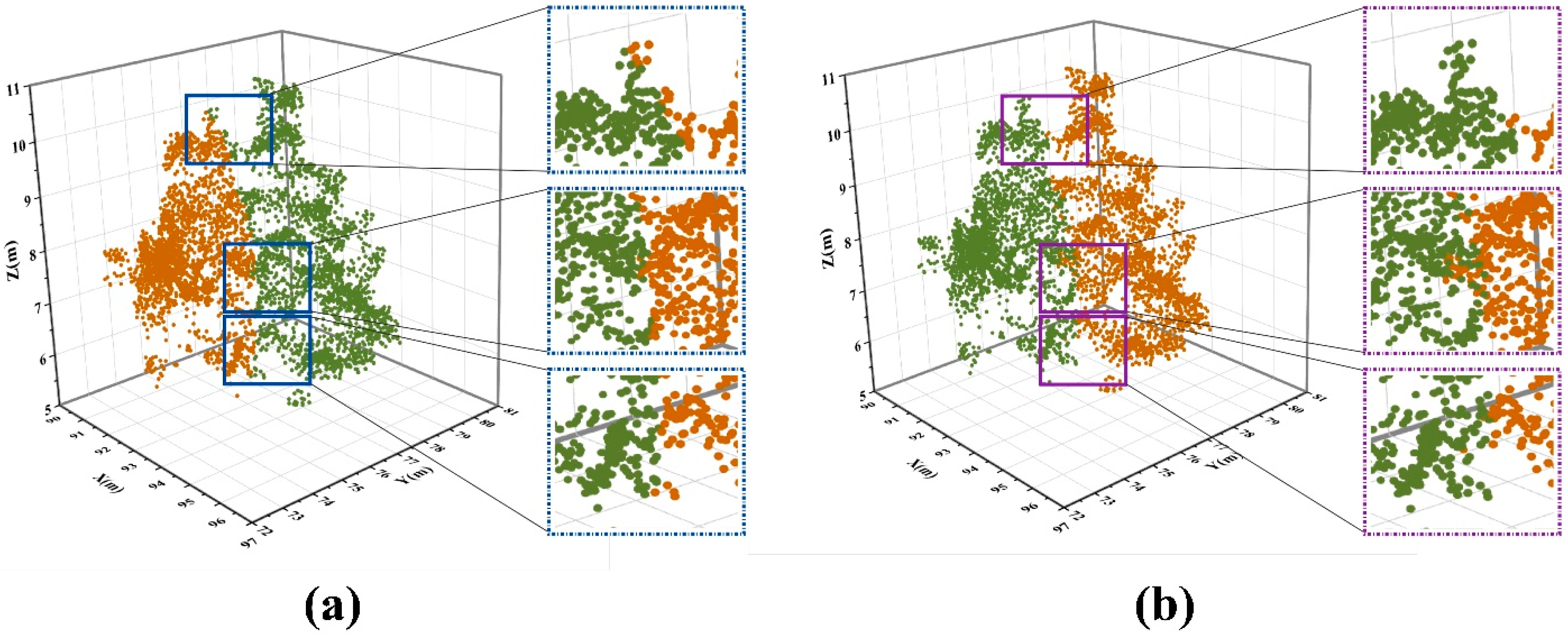
Once the number of subsamples of the under-segmented samples and their respective approximate centers are obtained, the under-segmented samples can be clustered and segmented based on GMM, using the number of subsamples as the number of clusters and the approximate center as the starting cluster center. Once the first segmentation is completed, the subsamples of the under-segmented samples can be obtained. However, due to numerous confounding factors such as local data defects caused by occlusion in the under-segmented samples, clustering based solely on approximate centers can make the results significantly defective, as shown in Figure 8a. Therefore, based on the previous method, thirteen-dimensional feature parameters of each subsample are extracted from the first segmentation, before the class of the subsample is determined using the trained SOM for classifying normally segmented samples and the optimal covariance matrix ∑jbest is matched for each subsample according to their class. Once the optimal covariance matrix of the corresponding class is matched for each subsample, the parameters of the GMM composed of the under-segmented samples can be calculated again according to the optimal covariance matrix, so as to finely segment the under-segmented samples against the uncertainty of the point cloud distribution of the same class, as shown in Equation (17):
j = i = 1 n γ i j ( X i μ j ) ( X i μ j ) T i = 1 n γ i j + j b e s t j 1 η · S i m i l a r i t y ( j 1 , j b e s t ) S i m i l a r i t y ( j 1 , j b e s t ) = 1 2 | | j b e s t j 1 | | F | | j 1 | | + | | j b e s t | |
The last compensation term is added to the covariance matrix of the jth sub-distribution model at each iteration of the calculation: first, the similarity of the sub-model covariance matrix to the optimal covariance matrix of the class to which it belongs is calculated, using the inverse as the scale factor; then, the new covariance matrix from each iteration is compensated according to the difference matrix and the scale factor, so that the covariance matrix of this sub-distribution model increasingly approximates the optimal covariance matrix of its kind. The value of the hyperparameter η is inversely related to the compensation effort. The larger the η, the smaller the compensation effort at each iteration, and vice versa.
Guided by the optimal distribution uncertainty represented by the optimal covariance matrix, the distribution uncertainty of each sub-model in the GMM composed of under-segmented samples is closest to the optimal distribution uncertainty of its corresponding class. This way, a more ideal segmentation state is reached, as shown in Figure 8b, optimizing the segmentation of under-segmented samples and achieving better ITS results.

2.8. Validation Procedure

The results of ITS experiments were evaluated in terms of canopy delineation accuracy (CDA) and forest parameter accuracy (FPA).
CDA evaluates the segmentation results of individual tree canopies as correctly segmented, expressed as TP (True Positive); under-segmented, i.e., a tree is incorrectly partitioned to a neighboring tree, expressed as FN (False Negative), and over-segmented, i.e., an individual tree sample is incorrectly segmented into multiple individual trees, expressed as FP (False Positive). We counted the ITS results of six sample squares and obtained the TP, FN, and FP. Using these values, we calculated the Recall, which is used to represent the detection rate of trees, and Precision, which is used to represent the correct rate of tree segmentation. We also calculated the F-score to evaluate the overall accuracy that considers the wrong and missed scores [46], as shown in the following equation:
Recall = T P T P + F N
Precision = T P T P + F P
F - score = 2 · Recall · Precision Recall + Precision
We manually measured the crown width of the samples in the sample square based on the collected point cloud data, using the open source software Cloud Compare as a reference value. We calculated the crown width of the segmented individual samples with our algorithm as the estimated value, linearly regressed the reference and estimated values, and estimated the FPA with the statistical metrics from linear regression to help assess the effectiveness of the segmentation algorithm [23,47].

3. Result

3.1. ITS Results Based on MS

After pre-processing the sample point cloud data, we performed preliminary ITS on the canopy point cloud using the MS algorithm. The ITS results of the ten sample plots by MS algorithm are shown in Table 3. The experimental plots in Trento had a high proportion of coniferous species and the canopy was mostly spiky, which was easy to detect. However, it was difficult to determine the appropriate bandwidth for MS-based ITS because of the high crown density and complex variety with different heights and crown widths. The MS algorithm is less flexible and less able to deal with these kinds of data. There were a lot of under-segmented samples. The overall accuracy was very low. On the contrary, although the experimental plot in Qingdao also had more tree species and a mixed morphology, the lower crown density gave it a better segmentation result.

3.2. SVM and SOM Classification Results

After segmenting individual trees by MS, we extracted the thirteen-dimensional feature parameters of all samples, then built a training set and a test set with some of the samples for then binary classification of normally segmented and abnormally segmented samples. In the Trento dataset, the training set consisted of 119 abnormally segmented samples and 148 normally segmented samples, totaling 267. The test set consisted of 102 abnormally segmented samples and 176 normally segmented samples, totaling 278. Moreover, in the Qingdao dataset, the training set consisted of 39 abnormally segmented samples and 117 normally segmented samples, totaling 156. The test set consisted of 34 abnormally segmented samples and 140 normally segmented samples, totaling 174. We also mapped the features of the normally segmented and abnormally segmented sample sets so classified by SOM, dividing the abnormally segmented sample set into an under-segmented subsample set and an over-segmented subsample set. In addition, we assigned an arbitrary number of classes for the normally segmented sample set by determining their approximation according to their respective features.
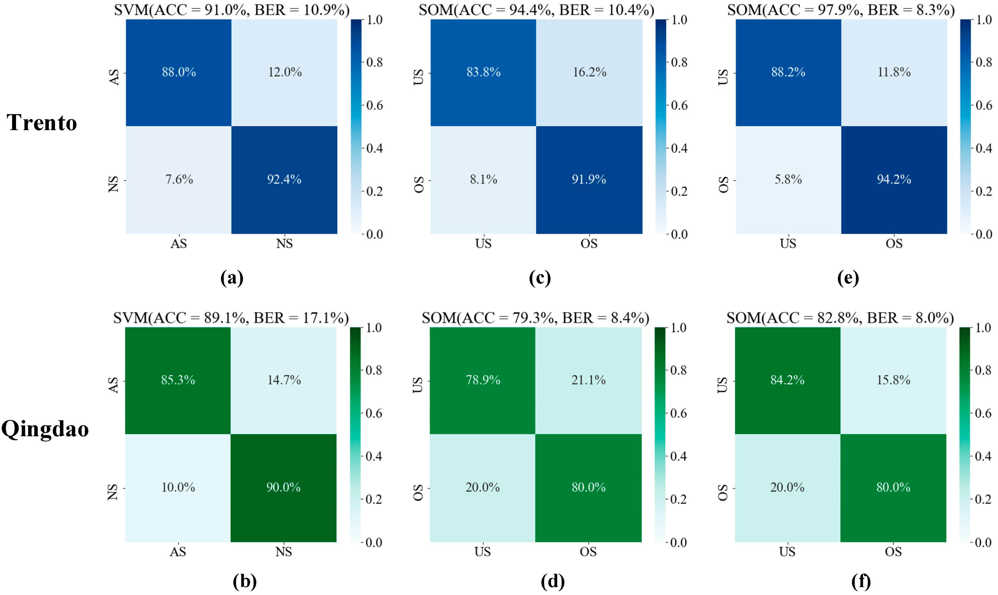
The SVM classification results in the experiment are shown in the confusion matrix in Figure 9a,b, and the ACC of Trento dataset was as high as 91.0% with a BER of 10.9%. Moreover, the ACC of Qingdao dataset was also respectable, reaching 89.1%. However, the small base of abnormally segmented samples in the Qingdao dataset led to a high BER of 17.1%. The less desirable ACC in the Qingdao dataset in the subsequent SOM classification was mainly due to this reason as well.
The SVM classification results were further classified by SOM and experimented in two ways: in the former, SOM was directly used to classify the SVM classification results, in the latter, SOM was trained on the SVM training dataset before it was used for further classification. In both datasets, the second approach exhibited a higher accuracy, probably due to the following reasons: the presence of some normally segmented samples in the SVM classification results may have affected the topology of the feature space for distinguishing under-segmented and over-segmented samples, accordingly, the accuracy of direct SOM classification. Better results should be achieved if the SOM is trained on the noise-free training data used by SVM to arm it with a good feature space structure before the SVM classification results are further classified on this basis.

3.3. GMM-Optimized Segmentation Results

After extracting the under-segmented samples and classifying the normally segmented samples according to their morphological features, we determined the number of sub-samples and the center position of the under-segmented samples using a density peak point clustering-based method, then optimized the segmentation by GMM. Figure 10a–d presents the optimization results for some of the sample plots, and Figure 10e–l presents the results for some of the under-segmented samples after optimized segmentation by GMM.
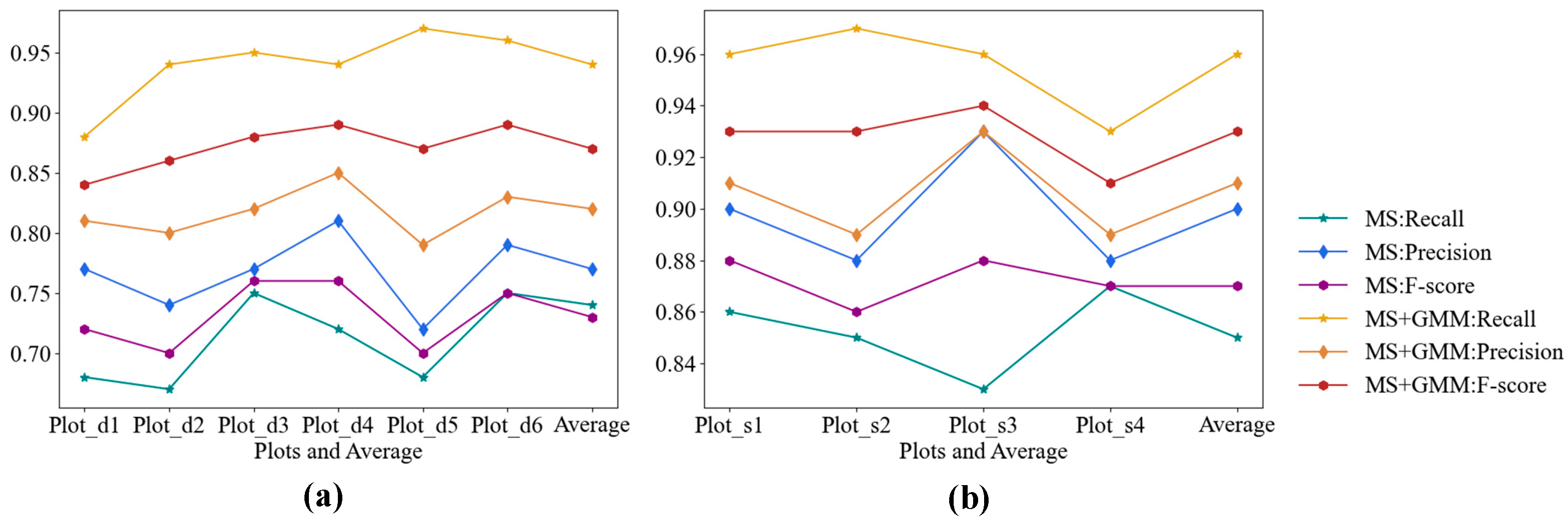
The final CDA assessment results for the ten plots are shown in Table 4. Compared with the previous MS-only segmentation method, the average Recall in the Trento dataset was improved by 20 percentage points, the average Precision was improved by 5 percentage points, and the average F-score was improved by 14 percentage points. In addition, the average Recall in the Qingdao dataset was improved by 11 percentage points, the average Precision was improved by 1 percentage points, and the average F-score was improved by 6 percentage points.
From the line graph drawn with the Recall, Precision, F-score, and average values of the sample plots shown in Figure 11, it can clearly be seen that the segmentation result by GMM was much better than when MS was used alone. As our algorithm involves optimized segmentation of under-segmented samples, and Recall reflects the detection rate of trees, it was also obvious that GMM-optimized segmentation improved Recall the most, followed by the F-score that considers both Recall and Precision. Precision was the least improved as it is related to the number of over-segmented samples.
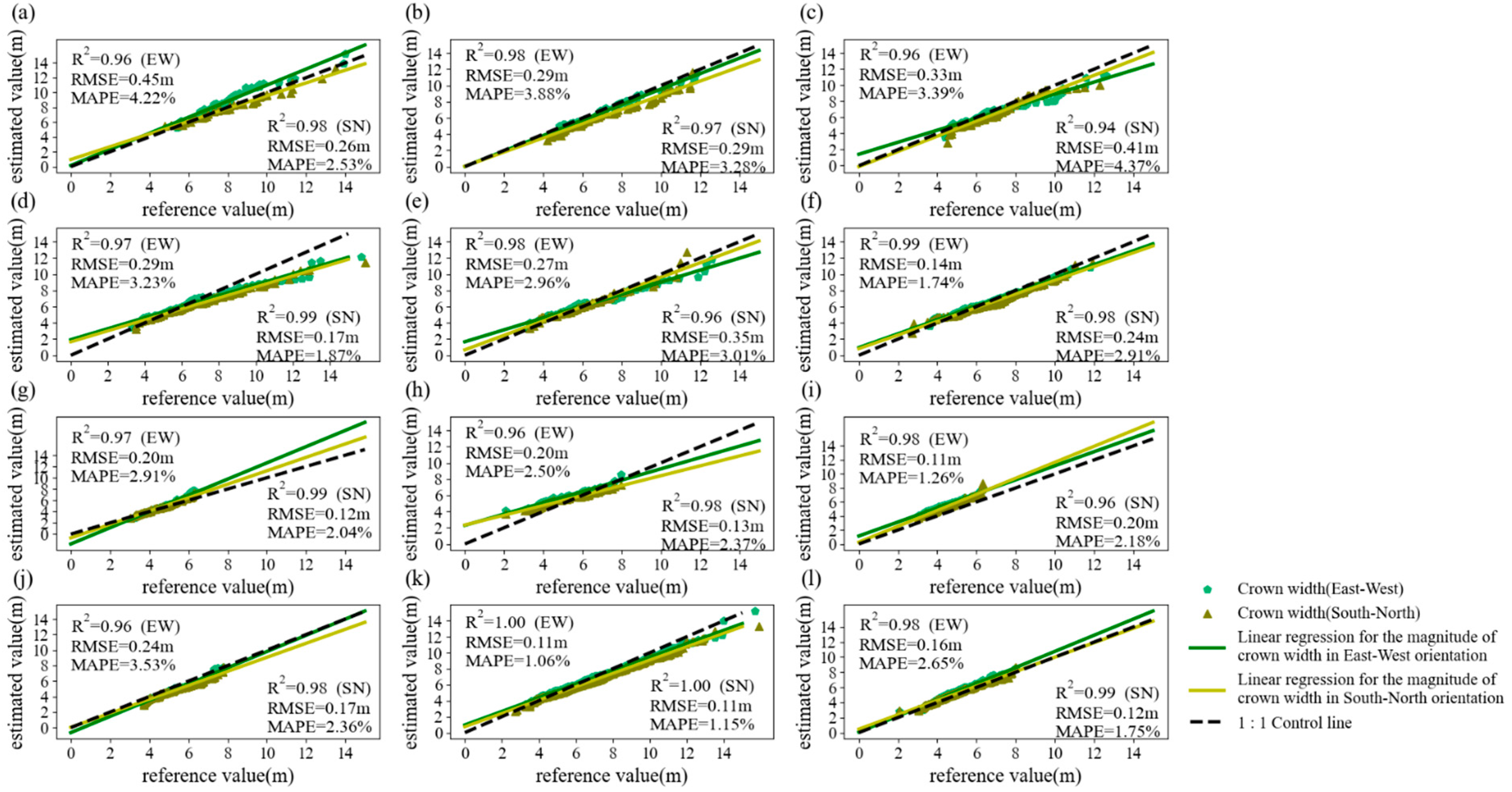
To check the overall segmentation quality, we calculated the crown width of the final ITS results of the ten sample plots according to their final ITS results as the estimated value, manually measured the crown width of individual trees in the point cloud as the reference value, and linearly regressed the estimated and reference values to verify the segmentation quality from the FPA perspective. Although real-place measurement was impossible due to practical restrictions, as the canopies in the experimental sample plots are mostly spiky and slender, subcanopy stands could still be clearly seen from a top view. It was hard to normally scan a few of the obstructed subcanopy stands by airborne LiDAR. The individual tree information obtained by visually and manually measured point cloud, although of limited accuracy, can still be used as reference values of ITS results. The linear regression results for the ten plots are shown in Figure 12. From the R2 values, there was a strong correlation between the estimated values calculated by the segmentation algorithm and the reference values. Despite the large span of crown width for all sample plots due to the diversity of stands, the overall RMSE and MAPE were low. In the Trento dataset, as shown in Figure 12a–f, the maximum RMSE and MAPE of the east–west crown width fell on Plot_s1, being 0.45 m and 4.22%; the maximum RMSE and MAPE of the north–south crown width fell on Plot_s3, being 0.41 m and 4.37%. Moreover, in the Qingdao dataset, as shown in Figure 12g–j, the maximum RMSE and MAPE of the east–west crown width fell on Plot_s4, being 0.24 m and 3.53%; the maximum RMSE of the north–south crown width fell on Plot_s3, being 0.20 m and the maximum MAPE fell on Plot_s2, being 2.37%. This indicates that the overall segmentation quality of the experimental sample plots was good.

4. Discussion

The MS algorithm has some disadvantages in segmenting individual trees due to its own limitations. First, as a method that relies on local density and height extremes to locate the vertex of individual trees, MS has some difficulty in detecting individual trees that lack significant canopy vertex features. Second, the bandwidths in the horizontal domain, hr, and that in the vertical domain, hs, determine the size of the search area. When the bandwidth is too small, the search field of view will be small, too. The algorithm will be unable to obtain sufficient effective information, so it tends to entangle on local details and split an individual tree into multiple homogeneous groups, thus leading to over-segmentation. When the bandwidth is too large, the search field of view will be large, too. The algorithm tends to ignore most of the underlying structure of the data and include many neighboring individual trees into the same homogeneous group, thus leading to under-segmentation. Furthermore, even with an appropriate bandwidth, a canopy can also be included into the same homogeneous group as a neighboring subcanopy (Figure 7e).
When used for ITS, the MS algorithm based on fixed bandwidth is more suitable for single stands. It performs less effectively when used for multistoried mixed forests with complex spatial structure such as that used in our experiment. To optimize the segmentation of under-segmented samples and improve the individual tree detection rate, we extracted the under-segmented samples, obtained their individual tree composition from density information, and segmented them again using GMM clustering.

4.1. Under-Segmentation Sample Extraction

In the proposed algorithm, under-segmented samples are obtained in two steps. First, abnormally segmented samples are separated by training SVM. Then, the samples divided into under-segmented and over-segmented samples using SOM. Therefore, the accuracy of both SVM and SOM makes a great difference to the accurate acquisition of under-segmented samples.
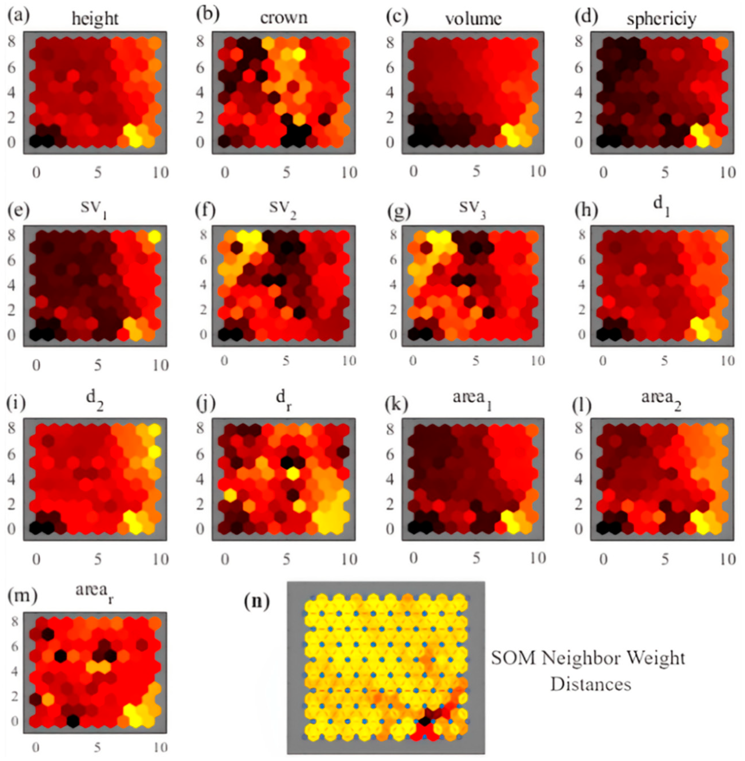
Figure 13 shows the feature space distribution of SOM used to divide abnormally segmented samples into under- and over-segmented samples. From the total distribution (Figure 13n), it can be seen that the feature space is clearly divided into two parts by the dark area. The smaller part represents the under-segmented feature distribution, whereas the over-segmented samples have a broader feature distribution due to diverse morphology [48]. By comparing the feature space distribution of individual feature parameters (Figure 13a–m) with the overall feature space distribution (Figure 13n), it can be seen that the feature space distribution of height, volume, d1, d2, sphericity, area1, area2, and arear is the most similar to the overall feature space distribution, so it can be decided that these eight feature parameters are the main basis for SOM classification. Among these eight feature parameters, the feature space distribution of dr, area1, area2, and arear is more chaotic. So the following conclusions can be drawn:
  • dr differs too less able to represent features than d1 and d2. Calculating dr would interfere with the construction of a clear feature space based on canopy length features;
  • arear is almost as able as, or even better able than, area1 and area2 to represent features. Calculating arear helps to construct a clear feature space based on canopy area features;
  • The feature space distribution of crown, sv1, sv2, and sv3 is too chaotic to be used as effective features for classification.
As for SVM classification, the gap between normally segmented samples and under-segmented samples is similar. The main judgment features are still canopy length features and canopy area features, which also make a great difference to the classification of under- and over-segmented samples. Therefore, the algorithm needs to enhance the extraction accuracy of these two types of features. This will effectively improve not only the classification of normal and abnormal samples by SVM, but also the classification of under- and over-segmented samples by SOM.

4.2. GMM-Optimized Segmentation

As the size of the homogeneous groups divided by MS clustering is limited by the bandwidth parameters, this method can hardly applied to canopies with large morphological differences. Ferraz et al. identified the upper canopy, lower canopy, and ground vegetation by mapping the height histograms of forest plots, and then segmented them by MS with different bandwidths [41]. However, when the vertical structure of the forest stand is less layered, it was difficult to achieve a clear hierarchy. In addition, the density distribution of canopy point clouds acquired by airborne LiDAR differs obviously on different vertical layers [42,49]. Therefore, in optimizing under-segmented samples, GMM is chosen to approximate the spatial structure of the canopy. Given that the probability density of Gaussian distribution gradually reduces from the center outwards, when using GMM to optimize under-segmented samples, it is necessary to roughly locate the center of the subsamples in the under-segmented samples and use it to initialize the clustering center. Based on canopy point clouds acquired by airborne LiDAR, local density peaks tend to occur near the top of the canopy [50]. For the ground projection point set of a canopy point cloud, directly obtaining the density distribution information of the whole canopy by calculating its single point Gaussian kernel density (Figure 7c,g) can avoid the information loss that would otherwise arise when the local search in MS is used. In the meantime, dropping the information on the extremes of height can avoid the missed detection of a sub-canopy layer caused by large height differences (Figure 7e). By detecting density peak density points, we can usually obtain multiple clusters of peak points (Figure 7c,g), and calculate the mean point of each cluster, which can be approximated as the center position of the canopy in the horizontal plane. Compared to the MS algorithm that detects individual trees by forced positioning of the vertex, this approach is more flexible for canopies that lack significant vertex features.
However, this method also has some instability. In Equation (17), we added a compensation term to the covariance matrix for each subsample iteration to compensate for the error caused by randomness in probabilistic clustering. Since this compensation term is based on the similarity between the optimal covariance matrix and the covariance matrix in the iteration to calculate the compensation amount, the similarity of the two matrices will change after each iteration. However, the hyperparameter η is a fixed value, so it is not flexible enough in the face of dynamic similarity. In the solution space, this unstable search pace may make the algorithm difficult to converge. Therefore, the setting of hyperparameter η is also very important, which will be improved in the future.

4.3. Analysis of Failure Cases

The proposed method is subject to the following failure cases:
i.
It cannot extract under-segmented samples due to misclassification by SVM or SOM and cannot optimize them by GMM;
ii.
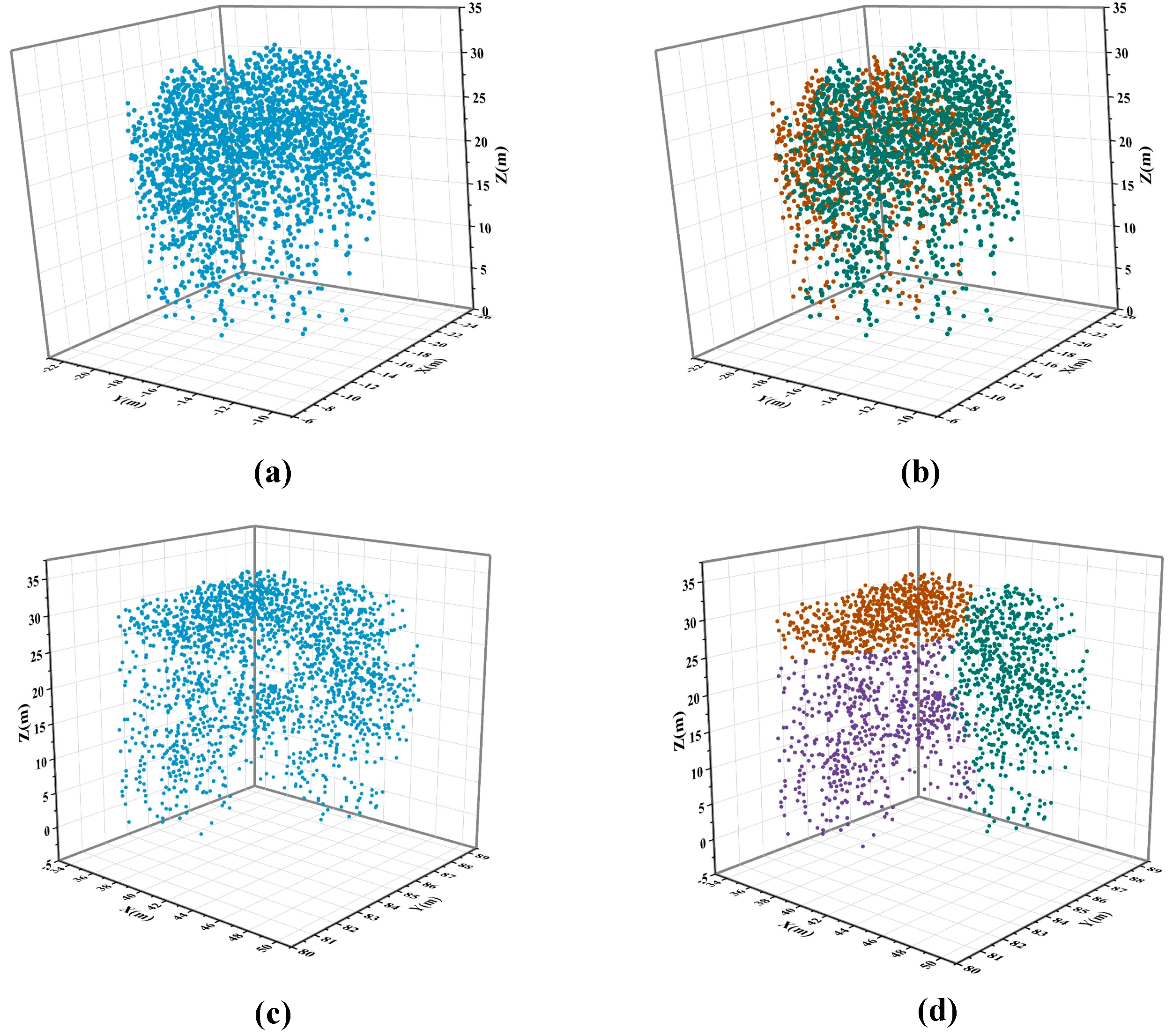
It determines the number of subsamples or calculates the center point position incorrectly as the density peak points are too centralized or decentralized, eventually leading to failure of optimized segmentation (Figure 14a,b);
iii.
It can calculate the number of subsamples and the approximate centers, but cannot optimize the under-segmented samples correctly (Figure 14c,d).
From the statistics of the failure results (Table 5), cases (i) and (ii) are the main reasons for the failure of optimized segmentation in Trento dataset. In general, as long as the number of subsamples in the under-segmented samples and their respective approximate centers are correctly calculated, GMM can basically segment them correctly and optimally. For some cases of segmentation boundary anomalies, a compensation term (Equation (17)) with the approximate morphology as a reference is added to obtain more accurate segmentation results. However, given the discreteness and uneven density distribution of the point cloud of canopies, even if the center points of the subsamples are found correctly, the true distribution of individual tree point clouds do not necessarily conform to a better GMM probability density distribution. So, failure cases similar to (iii) can still arise. Although the stand density in Qingdao dataset was low, compared with Trento dataset, the tree species complexity was higher, and the proportion of coniferous forests was lower. This more chaotic canopy structure makes it more difficult to detect approximate centers and subsequent optimized segmentation. This is also why in the Qingdao dataset failure cases, case (ii) and (iii) dominated.

5. Conclusions

In order to improve the ITS accuracy for high-density mixed forest areas, this study proposed an ITS method for forest airborne point clouds based on a Gaussian mixture model. The method builds on MS to extract under-segmented samples by integrated learning and classify normally segmented samples by morphological similarity. Guided by the approximate distribution uncertainty of similar normally segmented samples, the distribution uncertainty of each sub-model in the Gaussian mixture model to which the under-segmented samples belong is calculated and used to re-segment the under-segmented samples. The experiment was conducted with two datasets of airborne LiDAR data from a total of ten plots. The segmentation quality was assessed from both CDA and FPA perspectives. The results showed that the proposed method well improved the under-segmentation in the ITS of high-density, multistoried mixed forests, and achieved a better segmentation accuracy. However, for some under-segmented samples with particularly large density differences in vertical structure, our algorithm could hardly segment them normally. This problem will be further studied and optimized in the future and the combination of deep learning techniques to explore the deeper characteristics of canopy point clouds and optimize segmentation in higher dimensions will be considered.

Author Contributions

Conceptualization, J.W. and Z.L.; Methodology, Z.Z.; Validation, Z.Z.; Formal analysis, Y.Z.; Investigation, Z.L.; Data curation, A.H.; Writing—original draft, Z.Z.; Writing—review & editing, J.W., Z.L. and Y.Z.; Visualization, Z.Z.; Supervision, R.W.; Funding acquisition, J.W. All authors have read and agreed to the published version of the manuscript.

Funding

This research was supported by Introduction plan of high-end foreign experts (Grant No. G2021025006L) and Shandong University of Science and Technology “College Students ‘Innovation and Entrepreneurship Training Program” (Grant No. 202210424061).

Data Availability Statement

The data used to support the findings of this study are available from the corresponding author upon request.

Acknowledgments

We thank the Interreg Alpine Space Project for data support (Project number 2-3-2-FR). Moreover, we want to thank the anonymous reviewers for their relevant and in-depth comments.

Conflicts of Interest

The authors declare no conflict of interest.

References

  1. Yu, X.; Kukko, A.; Kaartinen, H.; Wang, Y.; Liang, X.; Matikainen, L.; Hyyppä, J. Comparing features of single and multi-photon lidar in boreal forests. ISPRS J. Photogramm. Remote Sens 2020, 168, 268–276. [Google Scholar] [CrossRef]
  2. Tang, Z.; Xia, X.; Huang, Y.; Lu, Y.; Guo, Z. Estimation of National Forest Aboveground Biomass from Multi-Source Remotely Sensed Dataset with Machine Learning Algorithms in China. Remote Sens. 2020, 14, 5487. [Google Scholar] [CrossRef]
  3. Shao, J.; Zhang, W.; Mellado, N.; Wang, N.; Jin, S.; Cai, S.; Yan, G. SLAM-aided forest plot mapping combining terrestrial and mobile laser scanning. ISPRS J. Photogramm. Remote Sens. 2020, 163, 214–230. [Google Scholar] [CrossRef]
  4. Nguyen, V.T.; Fournier, R.A.; Côté, J.F.; Pimont, F. Estimation of vertical plant area density from single return terrestrial laser scanning point clouds acquired in forest environments. Remote Sens. Environ. 2022, 279, 113115. [Google Scholar] [CrossRef]
  5. Liu, X.; Ma, Q.; Wu, X.; Hu, T.; Liu, Z.; Liu, L.; Su, Y. A novel entropy-based method to quantify forest canopy structural complexity from multiplatform lidar point clouds. Remote Sens. Environ. 2022, 282, 113280. [Google Scholar] [CrossRef]
  6. Baltsavias, E.P. Airborne laser scanning: Basic relations and formulas. ISPRS J. Photogramm. Remote Sens. 1999, 54, 199–214. [Google Scholar] [CrossRef]
  7. Kim, C.; Habib, A.; Pyeon, M.; Kwon, G.R.; Jung, J.; Heo, J. Segmentation of Planar Surfaces from Laser Scanning Data Using the Magnitude of Normal Position Vector for Adaptive Neighborhoods. Sensors 2016, 16, 140. [Google Scholar] [CrossRef] [Green Version]
  8. Wang, R.; Hu, Y.; Wu, H.; Wang, J. Automatic extraction of building boundaries using aerial LiDAR data. J. Appl. Remote Sens. 2016, 10, 016022. [Google Scholar] [CrossRef]
  9. Lefsky, M.A.; Cohen, W.B.; Parker, G.G.; Harding, D.J. Lidar Remote Sensing for Ecosystem Studies. BioScience 2002, 52, 19–30. [Google Scholar] [CrossRef]
  10. Wulder, M.A.; White, J.C.; Nelson, R.F.; Næsset, E.; Ørka, H.O.; Coops, N.C.; Hilke, T.; Bater, C.W.; Gobakken, T. Lidar Sampling for Large-Area Forest Characterization: A Review. Remote Sens. Environ. 2012, 121, 196–209. [Google Scholar] [CrossRef]
  11. Cao, W.; Wu, J.; Shi, Y.; Chen, D. Restoration of Individual Tree Missing Point Cloud Based on Local Features of Point Cloud. Remote Sens. 2022, 14, 1346. [Google Scholar] [CrossRef]
  12. Zhao, Y.; Ma, Y.; Quackenbush, L.J.; Zhen, Z. Estimation of Individual Tree Biomass in Natural Secondary Forests Based on ALS Data and WorldView-3 Imagery. Remote Sens. 2022, 14, 271. [Google Scholar] [CrossRef]
  13. Unger, D.; Hung, I.; Brooks, R.E.; Williams, H.M. Estimating number of trees, tree height and crown width using Lidar data. GIScience Remote Sens. 2014, 51, 227–238. [Google Scholar] [CrossRef]
  14. Ene, L.T.; Gobakken, T.; Andersen, H.E.; Næsset, E.; Cook, B.D.; Morton, D.C.; Babcock, C.; Nelson, R. Large-scale estimation of aboveground biomass in miombo woodlands using airborne laser scanning and national forest inventory data. Remote Sens. Environ. 2017, 186, 626–636. [Google Scholar] [CrossRef]
  15. Schlund, M.; Erasmi, S.; Scipal, K. Comparison of Aboveground Biomass Estimation from InSAR and LiDAR Canopy Height Models in Tropical Forests. IEEE Geosci. Remote Sens. Lett. 2020, 17, 367–371. [Google Scholar] [CrossRef]
  16. Aaron, J.; Baoxin, H.; Jili, L.; Linhai, J. Improving the efficiency and accuracy of individual tree crown delineation from high-density LiDAR data. Int. J. Appl. Earth Obs. Geoinf. 2014, 26, 145–155. [Google Scholar]
  17. Duncanson, L.I.; Cook, B.D.; Hurtt, G.C.; Dubayah, R.O. An efficient, multi-layered crown delineation algorithm for mapping individual tree structure across multiple ecosystems. Remote Sens. Environ. 2014, 154, 378–386. [Google Scholar] [CrossRef]
  18. Mongus, D.; Žalik, B. An efficient approach to 3D single tree-crown delineation in LiDAR data. ISPRS J. Photogramm. Remote Sens. 2015, 108, 219–233. [Google Scholar] [CrossRef]
  19. Liu, L.; Lim, S.; Shen, X.; Yebra, M. A hybrid method for segmenting individual trees from airborne lidar data. Comput. Electron. Agric. 2019, 163, 104871. [Google Scholar] [CrossRef]
  20. Liu, H.; Dong, P.; Wu, C.; Wang, P.; Fang, M. Individual tree identification using a new cluster-based approach with discrete-return airborne LiDAR data. Remote Sens. Environ. 2021, 258, 112382. [Google Scholar] [CrossRef]
  21. Douss, R.; Farah, I.R. Extraction of individual trees based on Canopy Height Model to monitor the state of the forest. Trees For. People 2022, 8, 100257. [Google Scholar] [CrossRef]
  22. Khosravipour, A.; Skidmore, A.K.; Isenburg, M. Generating spike-free digital surface models using LiDAR raw point clouds: A new approach for forestry applications. Int. J. Appl. Earth Obs. Geoinf. 2016, 52, 104–114. [Google Scholar] [CrossRef]
  23. Yun, T.; Jiang, K.; Li, G.; Eichhorn, M.P.; Fan, J.; Liu, F.; Chen, B.; An, F.; Cao, L. Individual tree crown segmentation from airborne LiDAR data using a novel Gaussian filter and energy function minimization-based approach. Remote Sens. Environ. 2021, 256, 112307. [Google Scholar] [CrossRef]
  24. Alon, A.S.; Enrique, D.F.; Drandreb, E.O.J. Tree Detection using Genus-Specific RetinaNet from Orthophoto for Segmentation Access of Airborne LiDAR Data. In Proceedings of the 2019 IEEE 6th International Conference on Engineering Technologies and Applied Sciences (ICETAS), Kuala Lumpur, Malaysia, 20–21 December 2019; pp. 1–6. [Google Scholar]
  25. Aubry-Kientz, M.; Dutrieux, R.; Ferraz, A.; Saatchi, S.; Hamraz, H.; Williams, J.; Coomes, D.; Piboule, A.; Vincent, G. A Comparative Assessment of the Performance of Individual Tree Crowns Delineation Algorithms from ALS Data in Tropical Forests. Remote Sens. 2019, 11, 1086. [Google Scholar] [CrossRef] [Green Version]
  26. Chen, Q.; Gao, T.; Zhu, J.; Wu, F.; Li, X.; Lu, D.; Yu, F. Individual Tree Segmentation and Tree Height Estimation Using Leaf-Off and Leaf-On UAV-LiDAR Data in Dense Deciduous Forests. Remote Sens. 2022, 31, 2787. [Google Scholar] [CrossRef]
  27. Amiri, N.; Polewski, P.; Heurich, M.; Krzystek, P. Adaptive stopping criterion for top-down segmentation of ALS point clouds in temperate coniferous forests. ISPRS J. Photogramm. Remote Sens. 2018, 141, 265–274. [Google Scholar] [CrossRef]
  28. Jaskierniak, D.; Lucieer, A.; Kuczera, G.; Turner, D.; Lane, P.N.J.; Benyon, R.G.; Haydon, S. Individual tree detection and crown delineation from Unmanned Aircraft System (UAS) LiDAR in structurally complex mixed species eucalypt forests. ISPRS J. Photogramm. Remote Sens. 2021, 171, 171–187. [Google Scholar] [CrossRef]
  29. Harikumar, A.; Bovolo, F.; Bruzzone, L. A Local Projection-Based Approach to Individual Tree Detection and 3-D Crown Delineation in Multistoried Coniferous Forests Using High-Density Airborne LiDAR Data. IEEE Trans. Geosci. Remote Sens. 2019, 57, 1168–1182. [Google Scholar] [CrossRef]
  30. Xu, S.; Ye, N.; Xu, S.; Zhu, F. A supervoxel approach to the segmentation of individual trees from LiDAR point clouds. Remote Sens. Lett. 2018, 9, 515–523. [Google Scholar] [CrossRef]
  31. Amr, A.; Rrn, A.; Rk, B. Individual tree detection from airborne laser scanning data based on supervoxels and local convexity. Remote Sens. Appl. Soc. Environ. 2019, 15, 100242. [Google Scholar]
  32. Yan, W.; Guan, H.; Cao, L.; Yu, Y.; Li, C.; Lu, J. A self-adaptive mean shift tree-segmentation method Using UAV LiDAR data. Remote Sens. 2020, 12, 515. [Google Scholar] [CrossRef] [Green Version]
  33. Estornell, J.; Hadas, E.; Martí, J.; López-Cortés, I. Tree extraction and estimation of walnut structure parameters using airborne LiDAR data. Int. J. Appl. Earth Obs. Geoinf. 2021, 96, 102273. [Google Scholar] [CrossRef]
  34. Sun, C.; Huang, C.; Zhang, H.; Chen, B.; An, F.; Wang, L.; Yun, T. Individual Tree Crown Segmentation and Crown Width Extraction From a Heightmap Derived From Aerial Laser Scanning Data Using a Deep Learning Framework. Front. Plant Sci. 2022, 13, 914974. [Google Scholar] [CrossRef] [PubMed]
  35. Dai, W.; Yang, B.; Dong, Z.; Shakerb, A. A new method for 3D individual tree extraction using multispectral airborne LiDAR point clouds. ISPRS J. Photogramm. Remote Sens. 2018, 144, 400–411. [Google Scholar] [CrossRef]
  36. Eysn, L.; Hollaus, M.; Lindberg, E.; Berger, F.; Monnet, J.M.; Dalponte, M.; Kobal, M.; Pellegrini, M.; Lingua, E.; Mongus, D.; et al. A Benchmark of Lidar-Based Single Tree Detection Methods Using Heterogeneous Forest Data from the Alpine Space. Forests 2015, 6, 1721–1747. [Google Scholar] [CrossRef] [Green Version]
  37. Li, Y.; Wang, J.; Li, B.; Sun, W.; Li, Y. An adaptive filtering algorithm of multilevel resolution point cloud. Surv. Rev. 2020, 53, 300–311. [Google Scholar] [CrossRef]
  38. Comaniciu, D.; Meer, P. Mean shift: A robust approach toward feature space analysis. IEEE Trans. Pattern Anal. Mach. Intell. 2002, 24, 603–619. [Google Scholar] [CrossRef] [Green Version]
  39. Fukunaga, K.; Hostetler, L.D. The estimation of the gradient of a density function, with applications in pattern recognition. IEEE Trans. Inf. Theory 1975, 21, 32–40. [Google Scholar] [CrossRef] [Green Version]
  40. Cheng, Y. Mean shift, mode seeking, and clustering. IEEE Trans. Pattern Anal. Mach. Intell. 1995, 17, 790–799. [Google Scholar] [CrossRef] [Green Version]
  41. Ferraz, A.; Bretar, F.; Jacquemoud, S.; Gonçalves, G.R.; Pereira, L.G.; Tomé, M.; Soares, P. 3-D mapping of a multi-layered Mediterranean forest using ALS data. Remote Sens. Environ. 2012, 121, 210–223. [Google Scholar] [CrossRef]
  42. Ferraz, A.S.; Saatchi, S.S.; Mallet, C.; Meyer, V. Lidar detection of individual tree size in tropical forests. Remote Sens. Environ. 2016, 183, 318–333. [Google Scholar] [CrossRef]
  43. Liang, X.; Litkey, P.; Hyyppa, J.; Kaartinen, H.; Vastaranta, M.; Holopainen, M. Automatic Stem Mapping Using Single-Scan Terrestrial Laser Scanning. IEEE Trans. Geosci. Remote Sens. 2012, 50, 661–670. [Google Scholar] [CrossRef]
  44. Sun, H.; Wang, S.; Jiang, Q. FCM-Based Model Selection Algorithms for Determining the Number of Clusters. Pattern Recognit. 2004, 37, 2027–2037. [Google Scholar] [CrossRef]
  45. Sun, W.; Wang, J.; Yang, Y.; Jin, F. Rock Mass Discontinuity Extraction Method Based on Multiresolution Supervoxel Segmentation of Point Cloud. IEEE J. Sel. Top. Appl. Earth Obs. Remote Sens. 2021, 14, 8436–8446. [Google Scholar] [CrossRef]
  46. Li, W.; Guo, Q.; Jakubowski, M.K.; Kelly, M. A New Method for Segmenting Individual Trees from the Lidar Point Cloud. Photogramm. Eng. Remote Sens. 2012, 78, 75–84. [Google Scholar] [CrossRef] [Green Version]
  47. Yin, D.; Wang, L. How to assess the accuracy of the individual tree-based forest inventory derived from remotely sensed data: A review. Int. J. Remote Sens. 2016, 37, 4521–4553. [Google Scholar] [CrossRef]
  48. Xiao, L.; Wang, K.; Teng, Y.; Zhang, J. Component plane presentation integrated self-organizing map for microarray data analysis. FEBS Lett. 2003, 538, 117–124. [Google Scholar] [CrossRef] [PubMed] [Green Version]
  49. Richardson, J.J.; Moskal, L.M. Strengths and limitations of assessing forest density and spatial configuration with aerial LiDAR. Remote Sens. Environ. 2011, 115, 2640–2651. [Google Scholar] [CrossRef]
  50. Paric, C.; Valduga, D.; Bruzzone, L. A Hierarchical Approach to Three-Dimensional Segmentation of LiDAR Data at Single-Tree Level in a Multilayered Forest. IEEE Trans. Geosci. Remote Sens. 2016, 54, 4190–4203. [Google Scholar]
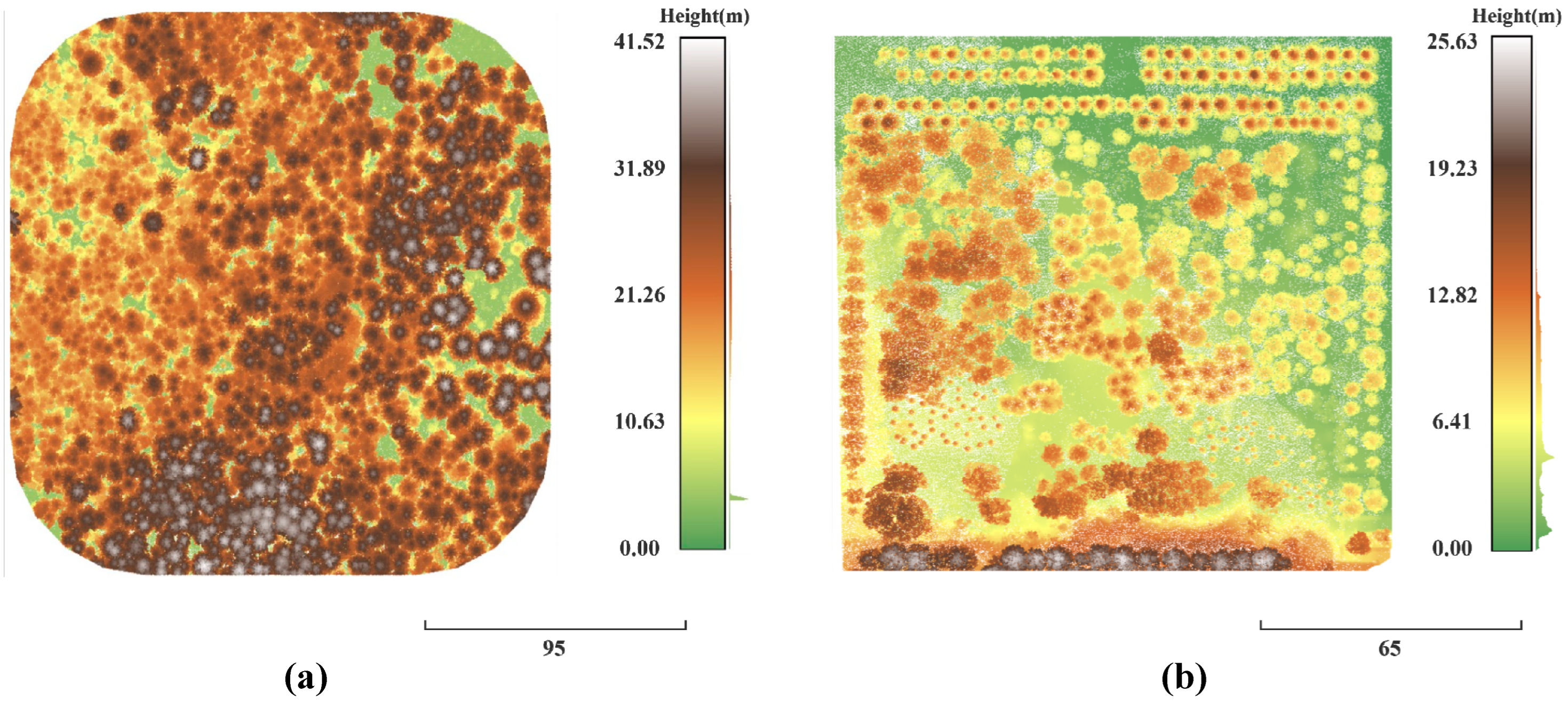
Figure 1. Schematic diagram of the point cloud data of the experimental area. (a) Trento; (b) Qingdao.
Remotesensing 14 06167 g001
Figure 2. Flowchart of the ITS optimization algorithm.
Remotesensing 14 06167 g002
Figure 3. Stepwise iterative search for individual tree vertices at seed points in the MS algorithm.
Remotesensing 14 06167 g003
Figure 4. (a) PCA-based calculation of the principal canopy direction to obtain the direction containing the maximum information, V1, and the next V2; (b) after the samples are projected in the principal direction, the polar differences of the projection point set transverse coordinates are d1, d2, and the internal area of the boundary of the projection point set is area1, area2, as shown in the gray shaded part of the diagram.
Remotesensing 14 06167 g004
Figure 5. Sample classification flow.
Remotesensing 14 06167 g005
Figure 6. Statistical Frobenius norm to rank abnormal samples.
Remotesensing 14 06167 g006
Figure 7. (a,b,e,f) Subsample approximate center points are calculated based on the homogeneous group composed of high-density points, and the clustering is performed by initializing the Gaussian mixture model clustering center with this; (c,d,g,h) density peak point detection based on the Gaussian kernel density of the sample ground projection point set, and the number of under-segmented sample subsamples is determined by calculating the CH score through iterative clustering. The scale of the color bar represents the Gaussian kernel density of the projection point.
Remotesensing 14 06167 g007
Figure 8. (a) After the first clustering segmentation, there is an obvious over division of the canopy on the right; (b) the re-clustering segmentation after adding the compensation term makes the two canopies more reasonably divided.
Remotesensing 14 06167 g008
Figure 9. (a,b) Results of the SVM classification of normally segmented samples and abnormally segmented samples; (c,d) SOM classification results of under-segmented and over-segmented samples, where (b) is the result of further classification of SVM test set classification results using SOM directly, and (e,f) is the result of further classification of SVM test set classification results after training SOM with samples from the SVM training set. (Note: AS is Abnormal segmentation, NS is Normal segmentation, and US is Under-segmentation, OS is Over-segmentation, ACC is Accuracy, and BER is Balanced Error Rate.).
Remotesensing 14 06167 g009
Figure 10. (ad) MS+GMM-optimized segmentation results for some samples; (el) Normal segmentation results obtained after GMM-optimized segmentation for some under-segmented samples after segmentation by the MS algorithm.
Remotesensing 14 06167 g010
Figure 11. The line graph of Recall, Precision, F-score, and average values of the ten sample plots under different treatments, which intuitively shows the superiority of our treatment over ITS using MS alone can visually represent that the treatment in this paper has obvious advantages over using MS alone for ITS. (a) Trento dataset; (b) Qingdao dataset.
Remotesensing 14 06167 g011
Figure 12. (af) Linear regression results of crown width measurements versus estimates obtained by algorithmic segmentation for the six sample plots from Plot_d1 to Plot_d6, (gj) Linear regression results of crown width measurements versus estimates obtained by algorithmic segmentation for the four sample plots from Plot_s1 to Plot_s4, where R2 (R Squared), RMSE (Root Mean Square Error) and MAPE (Mean Absolute Percentage Error) were used to evaluate the regression accuracy; (k) Linear regression results of all crown width measurements and estimates obtained by algorithmic segmentation for the six sample plots; (l) Linear regression results of all crown width measurements and estimates obtained by algorithmic segmentation for the four sample plots.
Remotesensing 14 06167 g012
Figure 13. Feature space distribution of SOM for under-segmented and over-segmented sample classification. (am) Relative distribution of each of the thirteen feature parameters in the feature space; (n) Distribution of all feature vectors in the feature space.
Remotesensing 14 06167 g013
Figure 14. Failure sample example. (a,b) Failure example of Case (ii): An approximate center is detected at the junction of two subsamples due to higher density at the junction of two canopies, resulting in failure of optimal segmentation; (c,d) Failure example of Case (iii): The approximate centers of the three samples are correctly detected, but the point cloud density distribution of the two subsamples on the left is too dense at the top and too scattered at the bottom, causing the GMM clustering to split them into two homogeneous groups at the top and bottom.
Remotesensing 14 06167 g014
Table 1. Tree information of the ten experimental plots.
DatasetProportion of
Species (%)
PlotNumbers
of Tree
Height (m)Crown Width (m)Crown Area (m2)
MaxMinAverageMaxMinAverageMaxMinAverage
Trento
(Complex)
Coniferous forest: 80%
Broadleaf forest:
20%
Plot_d14037.118.929.912.61.37.2123.811.348.1
Plot_d26332.917.725.611.22.16.698.910.838.1
Plot_d36434.719.328.511.92.46.6110.510.337.4
Plot_d410837.214.724.913.22.16.1137.88.836.7
Plot_d56234.120.524.813.32.97.1137.97.431.5
Plot_d611438.221.532.111.22.46.297.710.335.1
Total451
Qingdao
(Simple)
Coniferous forest: 45%
Broadleaf forest:
55%
Plot_s17610.87.08.26.33.04.6102.14.118.4
Plot_s26111.26.78.87.52.45.156.23.913.0
Plot_s38914.18.511.57.42.36.268.64.617.6
Plot_s47515.96.712.87.73.75.484.94.213.6
Total301
Table 2. Individual tree feature parameters.
IDParameter NameDescription
1heightThe height of the canopy
2crownThe average of the north–south and east–west widths of the trees
3volumeVolume of the canopy
4sphericitySphericity of the canopy point cloud
5sv1Canopy point cloud matrix singular value 1
6sv2Canopy point cloud matrix singular value 2
7sv3Canopy point cloud matrix singular value 3
8d1Maximum length of canopy horizontal projection
9d2Minimum length of canopy horizontal projection
10drThe ratio of d1 to d2
11area1The first principal component projects polygon area perpendicularly
12area2The second principal component projects polygon area perpendicularly
13arearThe ratio of area1 to area2
Table 3. ITS results by MS for the ten sample plots.
DatasetPlotNumber of DetectedTrue Positive (TP)False Negative (FN)False Positive (FP)RecallPrecisionF-Score
TrentoPlot_d135271380.680.770.72Average Recall0.74
Plot_d2574221150.670.740.70
Plot_d3624816140.750.770.76Average Precision0.77
Plot_d4967830180.720.810.76
Plot_d5584220160.680.720.70Average
F-score
0.73
Plot_d61088529230.750.790.75
Total41832412794
QingdaoPlot_s173661070.860.900.88Average Recall0.85
Plot_s25952970.850.880.86
Plot_s380741560.830.930.88Average Precision0.90
Plot_s474651090.870.880.87
Total2862574429 Average
F-score
0.87
Table 4. MS+GMM-optimized segmentation results for the ten sample plots.
DatasetPlotTrue Positive (TP)False Negative (FN)False Positive (FP)RecallPrecisionF-Score
TrentoPlot_d135580.880.810.84Average Recall0.94
Plot_d2594150.940.800.86
Plot_d3613140.950.820.88Average Precision0.82
Plot_d41026180.940.850.89
Plot_d5602160.970.790.87Average
F-score
0.87
Plot_d61095230.960.830.89
Total4262594
QingdaoPlot_s173370.960.910.93Average Recall0.96
Plot_s259270.970.890.93
Plot_s385460.960.930.94Average Precision0.91
Plot_s470590.930.890.91
Total2871429 Average
F-score
0.93
Table 5. Statistics of failure results.
Case(i)(ii)(iii)Total (i)(ii)(iii)Total
TrentoNumbers of tree128525Qingdao34714
Percentage48%32%20%100%21%29%50%100%
Publisher’s Note: MDPI stays neutral with regard to jurisdictional claims in published maps and institutional affiliations.