Technical Note

UBathy (v2.0): A Software to Obtain the Bathymetry from Video Imagery

by
Gonzalo Simarro
1,*,† and
Daniel Calvete
2,†
1
Marine Sciences Institute, CSIC, Passeig Maritim de la Barceloneta 37-49, 08003 Barcelona, Spain
2
Department of Physics, Polytechnic University of Catalonia–BarcelonaTech, Jordi Girona 1-3, 08034 Barcelona, Spain
*
Author to whom correspondence should be addressed.
These authors contributed equally to this work.
Remote Sens. 2022, 14(23), 6139; https://doi.org/10.3390/rs14236139
Submission received: 11 November 2022 / Revised: 25 November 2022 / Accepted: 26 November 2022 / Published: 3 December 2022
(This article belongs to the Special Issue Remote Sensing for Shallow and Deep Waters Mapping and Monitoring)

Abstract

:
UBathy is an open source software developed for bathymetry estimation from video images. The proposed scheme is based on extracting the wave modes from videos of the nearshore surface wave propagation. These videos can be formed either from raw camera images, which must have been previously calibrated, or from georeferenced planviews. For each wave mode extracted from the videos, the wave frequency and the spatially dependent wavenumbers are obtained. The frequencies and wavenumbers from different videos are used to estimate the bathymetry by adjusting the dispersion relationship for linear surface water waves. The bathymetry at different times can further be weighted and aggregated using the Kalman filter. The new software is suitable for Argus-type video monitoring stations and for moving cameras mounted on drones or satellites, and it is meant for users familiar with coastal image processing and suitable for non-experienced users. The software and an application example are available on the GitHub platform.

1. Introduction

Coastal zone management and research requires knowing the bathymetry and its changes [1,2]. Bathymetry has an immediate interest in decision making processes and, further, bathymetric timeseries allow to understand morphodynamic processes and to validate models which, in turn, are helpful to predict future changes and to analyze the impact of potential human actions [3,4]. Managers and scientists (marine geologists, coastal modelers, etc.), with different levels of technical background, are faced with the need for bathymetry, preferably with high frequency and at a low cost. The development of accurate, affordable and easy-to-use technologies can benefit all of them.
Techniques for direct bathymetry measurements such as bottom-contacting vehicles [5], swath-sounding sonar systems [6] or bathymetric LIDAR [7], produce very high quality bathymetry due to their high resolution. However, they are economically expensive and time-consuming techniques. Hence, they are only used at most a few times a year for a given site, except for very specific field campaigns. In the highly dynamic nearshore area, sporadic campaigns are important to obtain a rough estimate of the characteristics or the current state of the beach, but are of minor value to study its dynamics at the event scale.
The main alternative techniques to those listed above use sequential observations of the sea surface to infer the bathymetry from how it affects sea wave characteristics. These sequences of observations, which may come from satellite imagery [8], fixed coastal video monitoring stations [9], drones [10] or radars [11], are used to analyze the water wave propagation from which to infer the bathymetry. The methods are all based on the linear dispersion relationship, which relates the wave period and the wavelength (or, equivalently, the wave celerity) to the local water depth. In the nearshore zone, specific schemes have been developed to deal with non-monochromatic wave propagation in shallow waters, namely: cBathy [9], UBathy [12] and COCOs [13]. These algorithms, initially developed for videos obtained from fixed video monitoring systems (“Argus-like”, [14]), use videos of planviews (projections of the raw images into the mean water level plane) of around 10 min at 2 Hz and can also be applied to videos from radar [15] and drones [16]. The software proposed in this paper belongs to this category of schemes.
The cBathy algorithm [9] starts by transforming the time history of the intensity of each pixel into the frequency domain. To obtain the local water depth at a given point, cBathy considers a neighborhood and obtains the wave spatial pattern and the wave period through frequency-domain empirical orthogonal functions of the cross spectral matrices. The dispersion relationship then allows them to obtain estimates of the depth for each dominant frequency and, also, a weighted average of them. A Kalman time filter over the results of the available videos is required to obtain the bathymetry for successive dates (Figure 1A). The excellent results of cBathy clearly show the capability of using frequency and wavenumber values extracted from videos to estimate the bathymetry from the dispersion relationship when it is combined with a Kalman filter. The algorithm has recently been updated [17] to include, for instance, an adaptive scheme to determine the optimum size for the mentioned neighborhood, and it is available as open source Matlab toolbox.
The original UBathy algorithm [12] first splits the video in time to obtain sub-videos that are analyzed individually. The Hilbert transform of each sub-video is decomposed in space and time using empirical orthogonal functions (EOF). For the subsequent analysis, the modes whose temporal behavior is periodic are considered. For each of these modes, the wavenumber field is obtained locally fitting a plane to the phase of the spatial component of the mode. Finally, once all the sub-videos have been analyzed, the local depth is obtained by fitting the dispersion relationship to the set of pairs of wavenumbers and periods found at each point. The results with this algorithm show that the global analysis performed in the mode decomposition, while filtering the different wave constituents in the videos, allows a good extraction of wave numbers and periods and an improvement in the bathymetric estimation.
COCOs algorithm [13] splits the video in time and, for each sub-video, performs a space-time decomposition of the Hilbert transform of the signal, similar to UBathy. In this case, however, a dynamic mode decomposition (DMD) [18] is applied. This decomposition does not force orthogonality of the space components of the modes and ensures periodicity time-wise. The wavenumbers are obtained from the space components of the modes using in this case a two-dimensional fast fourier transform (2D-FFT) in a neighborhood whose size is obtained adaptively, and analyzing the wave celerity. By adjusting the Doppler-shifted linear dispersion relationship, a bathymetry and an associated current field are obtained for each sub-video. The estimation of the bathymetry is finally performed by applying a Kalman filtering to the resulting bathymetry of consecutive sub-videos and stopping the process once the convergence of the solution is found (Figure 1B). The COCOs results support the benefits of a global analysis of the wave modes as well as the capability of the Kalman filter for aggregating the bathymetry results within the video. This algorithm is available as open source Matlab toolbox.
The aim of this work is to present an improved version of the UBathy algorithm, including details of its open source software toolbox. The improvements include the application of robust principal component analysis (RPCA) [19] and DMD algorithms within the mode decomposition step, the use of adaptive neighborhoods for wavenumber and local water depth estimation, the outlier exclusion through the use of RANdom SAmple Consensus approach (RANSAC) [20] and, finally, the bathymetry aggregation through Kalman filtering. The work is complemented with the software, developed to be used by coastal community members not necessarily with programming expertise and, as developed in Python, with no additional licensing costs of proprietary tools. As new features, the software allows to obtain the bathymetry from video images covering different areas (with or without overlapping) and captured at different times. This allows large areas to be covered and avoids problems of camera synchronization. In addition, the videos can be based on calibrated raw images or georeferenced planviews (Figure 1C), allowing the use of multiple image sources (fixed stations, drones, satellites, etc.). The theoretical background and the main code characteristics are presented in Section 2. To illustrate the performance of UBathy, Section 3 presents and discusses the results for different videos obtained from a video monitoring station, including also some recommendations of use. The paper ends in Section 4 with some conclusions.

2. Methods and Software Description

UBathy has been developed to estimate the coastal bathymetry from the propagation of nearshore water waves as observed in video images. The main features of the software and the methodology are listed below.
  • Software characteristics. UBathy is an open source software developed in (also open source) Python3 and available at GitHub platform. It runs on any platform with a standard installation of Python3.9 (i.e., with “The Python Standard Library”) and OpenCV, NumPy, SciPy and matplotlib modules. The code is complemented with an example case so that any user can fully execute it. A guided example is included to run on Jupyter Notebook to facilitate its use to non-experienced users. The software is suitable for users who are familiar with coastal image processing.
  • Videos sources. A novel aspect of UBathy is that allows to directly process videos of raw camera images in addition to usual planview videos. In the first case (raw images), the videos can be acquired typically from fixed video monitoring stations (“Argus” type, [14]) but also from new CoastSnap stations [21]. For their processing, only the calibration of the camera is needed, without any further post-processing, together with the position of the mean water level at the time of the recording. Videos of planviews can normally come from fixed video monitoring stations or from the processing of drone flights. For planview videos it is necessary to know their georeference and the position of the mean water level.
  • Mode decomposition. The extraction of the wave modes and corresponding wave periods is performed by global analysis of the images. The software allows, at user’s request, to decompose the videos in time (wave periods) and space (wave phase) using EOF, following [12], or DMD [13]. In addition, the user can also reduce the signal noise of the videos by applying an RPCA [19]. The wavenumber estimation uses local adjustments of the wave phase.
  • Bathymetry estimation. The bathymetry is obtained by fitting the surface waves dispersion relationship with the wavenumbers and frequencies of the different modes, taking into account the different mean water levels. Another novel aspect of this software is the flexibility to obtain the bathymetry by assembling videos that: (1) cover different parts of the coastal area, (2) do not need to be recorded synchronously and with the same sea level and, (3) are made of different types of images (planviews and raw images). In addition to the bathymetry obtained from the above analysis, a Kalman filter is used to obtain the bathymetry at a given time by accumulating the results obtained up to that time.
The execution of the UBathy software is performed through the following steps:
Step 0: 
Video and data setup. The video frames, data for image georeferencing and mean water level during the recording of the videos are provided.
Step 1: 
Generation of meshes. Generation of the spatial meshes to express the mode decomposition, the wavenumbers and the bathymetry.
Step 2: 
Mode decomposition. The wave is decomposed into different modes, with the corresponding wave period and spatial phase.
Step 3: 
Wavenumber computation. The spatial phase of each mode is analyzed to extract the wavenumbers in the spatial domain.
Step 4: 
Bathymetry estimation. Estimation of the bathymetry from the set of periods and wavenumbers of different videos.
Step 5: 
Kalman filtering. Determination of the bathymetry evolution by time filtering the bathymetry results obtained from videos at different times.
Thereafter, Section 2.1 details the methodology and theoretical background for each of the different steps and Section 2.2 describes the software execution procedure, including the data structure, inputs and outputs.

2.1. Methodological Background

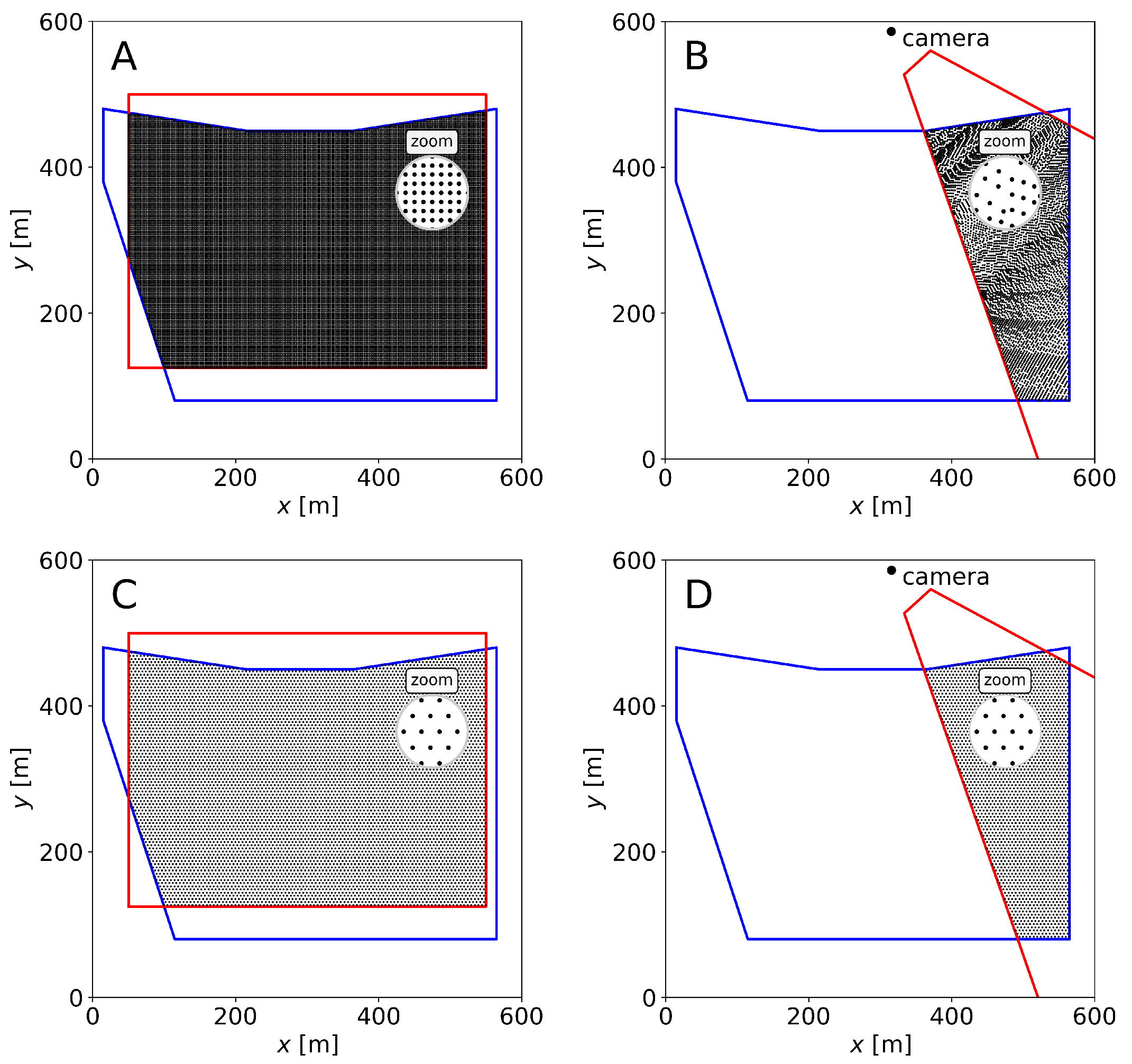
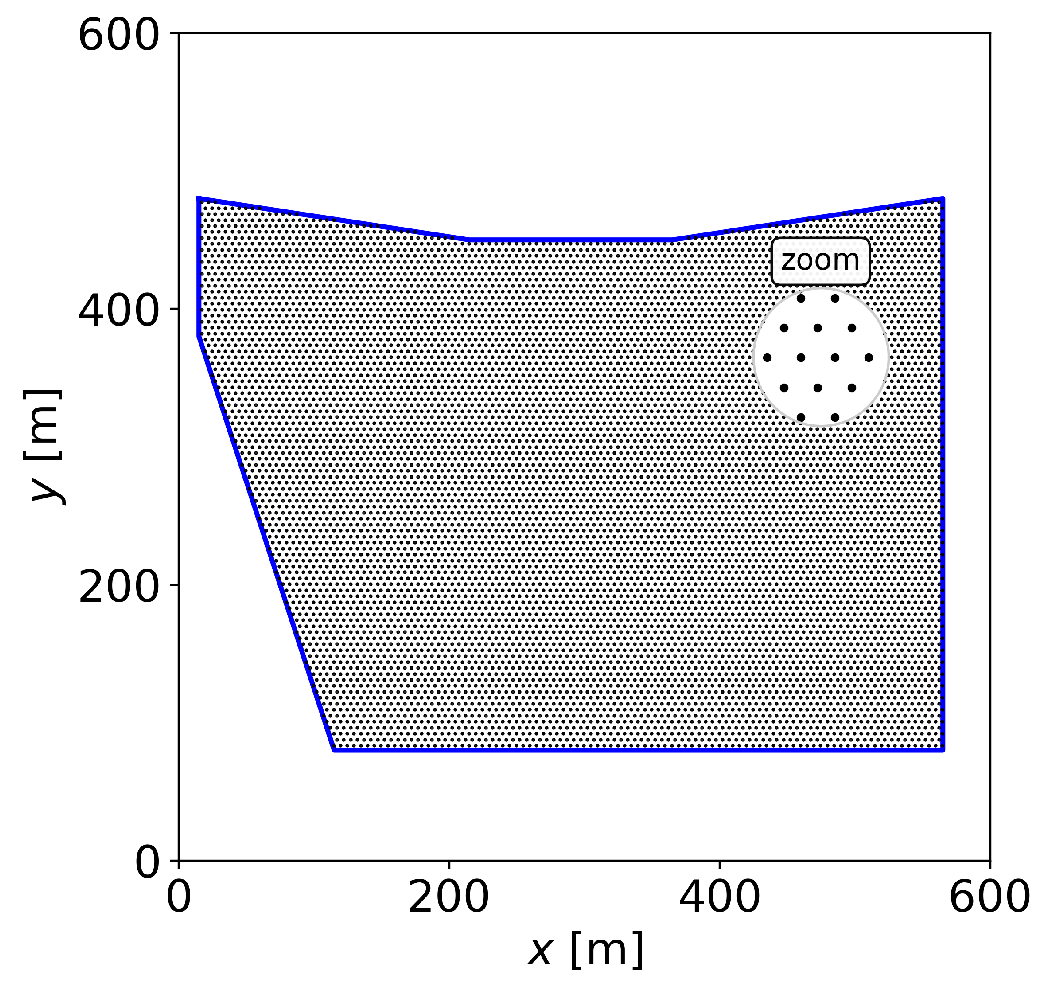
2.1.1. Generation of Meshes

For each video, the mesh where to obtain the modes (“M-mesh”) depends on whether the video is made of planview or raw (oblique) images. If it is made of planviews, the mesh are those x y - points of the planview which fall within the domain where the bathymetry is to be estimated (Figure 2A). When the video is made of raw images, the mesh is build as a set of x y - points within the bathymetry domain so that: (1) they correspond to integer-valued pixels of the raw images, so as to avoid later interpolations, and, (2) they resemble, as far as possible, a uniform equilateral triangle mesh of given resolution δ M , so as to avoid over-weighting the areas of the raw image where the pixel footprint in space is higher (Figure 2B). For each video, the mesh where to obtain the wavenumber k (the “K-mesh”) is made of the x y - points of a uniform equilateral triangle mesh of resolution δ K that fall both within the bathymetry domain and the x y - domain of the image, whether it is planview (Figure 2C) or raw (Figure 2D). Finally, the mesh for the bathymetry (“B-mesh”) are the x y - points of a uniform equilateral triangle mesh of resolution δ B within the bathymetry domain (Figure 3). This mesh is independent of the videos.

2.1.2. Mode Decomposition

Following Simarro et al. [12], each video is first cut to obtain, every time step Δ t (equal or higher than the time step between frames), a set of sub-videos of durations w 1 , w 2 , …(Figure 4). The signal in each sub-video is decomposed in space and time to estimate the wavenumbers and periods of the dominant wave components. Previously, the RPCA algorithm by [19] can be applied, with I M iterations, to remove noise from the signal. Further, the time Hilbert transform of the signal must be done before the mode decomposition to obtain a natural retrieval of phases [12]. Since the Hilbert transform generates overshoots at both ends of the time domain, the sub-videos are first increased at both ends with the expected maximum period ( T max , which is the maximum affection zone of the overshoots) and, once Hilbert-transformed, cropped back to w i (Figure 5).
Two different space-time mode decompositions are allowed for the Hilbert-transformed sub-videos: EOF [12] and DMD [13,22]. If EOF is applied, the modes that are considered for further analysis are those explaining a percentage of the total variance above a critical value ( v E 2.5 % ), having a proper temporal periodic behavior ( σ ω / ω 0.15 , following the notation in the original work) and with the period within a range [ T min , T max ] . If DMD is applied, the rank for the dimension reduction embedded in DMD must be provided ( r D 6 ) and the modes considered for further analysis are all those with a period in the range [ T min , T max ] . Either using EOF or DMD, the results for each sub-video is a set of modes. Each mode has a wave period and its complex-valued spatial component, given in the M-mesh, which can be represented by an amplitude and a phase (Figure 6).

2.1.3. Wavenumber Computation

For the modes obtained in the above decomposition, the wave wavenumbers, k, are computed using their period and spatial phase, which represents the phase of the wave (Figure 6). This step can be performed in different ways ([13] and references therein): from the phase gradient, performing spatial 2D-FFTs or, recalling the complex nature of the modes, through particle image velocimetry techniques (cross-correlation). A modification of the approach by Simarro et al. [12], based on computing the phase gradient, is considered here.
For each of the modes, the wavenumber k at each point P of the K-mesh is obtained by adjusting the phase locally to a plane. To achieve this, the phase values of the points of the M-mesh that are in a neighborhood of a given radius R K around point P are used (e.g., the points within the white circle in Figure 6A for the black dot). The values of R K are detailed below in this subsection. The phase values at these points are shifted to be centered around zero to avoid phase jumps at ± π (following the “phase fitting” method at Simarro et al. [12]) and then approximated with a plane k x x + k y y + α 0 , where k x , k y and α 0 are free coefficients. To remove the noise and the outliers in the phases, evident in some areas of Figure 6, a RANSAC approach [20] is applied maximizing the number of points with fitting errors below 0.25 rad 15 . The wavenumber is then
k = k x 2 + k y 2 .
Once the wavenumbers k of a mode of frequency ω have been computed, a first selection is performed using the parameter γ = ω 2 / ( g k ) , in which those with γ > 1.2 are discarded (gaps in Figure 7A,B). This parameter is also used to introduce two additional parameters that will be used later, in the estimation of the bathymetry, to evaluate the quality of the computed wavenumbers. For any point P of the K-mesh, the mean, μ γ and standard deviation, σ γ , of γ (Figure 7C,D), are computed with the values in a neighborhood of P of radius 0.5 λ , with λ = 2 π / k the estimated wavelength at P.
Regarding the radius R K , used to determine the neighborhood in which the phase is fitted to a plane, it has to be taken into account that very small neighborhoods make the results more sensitive to noise but large neighborhoods are likely to contain jumps of the phase. Given these limitations, it is convenient to use an R K that is, at most, of the order of one-half wavelength of the local wave. However, it is not known a priori since it depends on the wave period and the local (unknown) depth. In order to circumvent this problem, neighborhoods adapted to the different wave modes and depths are chosen.
As the frequency ω of a wave mode is known, the wavelengths corresponding to a set of depths in the range in which the bathymetry will be estimated are used; d min and d max , respectively, are the minimum and maximum obtainable depths; n K equispaced intermediate depths are defined in this range (see Figure 8, where n K = 3 )
d j = d min + j ( d max d min ) n K , j = 1 , , n K .
For each depth d j , the wavelength λ j = 2 π / k j is obtained from the dispersion relationship ω 2 = g k j tanh ( k j d j ) and the radius of the neighborhood is computed as R K , j = c K λ j , where c K is a factor of the wavelength that must be around 0.5 . Consequently, the values of k, γ , μ γ and σ γ will be obtained for each R K , j , assuming that larger radius will work better in deeper regions and vice versa. This approach follows a similar philosophy of adaptivity proposed by Gawehn et al. [13], Holman and Bergsma [17].

2.1.4. Bathymetry Estimation

The outcome of computing wavenumbers for all R K ’s of all modes of all sub-videos of all the videos from which a bathymetry will be computed, is a (very large, in general) set of tuples { x , y , ω , k , μ γ , σ γ , z s } , with z s the surface elevation, at each point of the K-meshes—recall that γ = ω 2 / ( g k ) is also provided. For the computation of the bathymetry, the tuples with the most reliable values of k are selected by requiring that
| γ μ γ | e B , σ γ e B ,
where e B 0.075 is a critical error (Table 1).
To estimate the bed elevation z b at a point P in the B-mesh, those tuples in a neighborhood of radius R B , which is discussed below, are used. First, an error is computed for a given depth z b of each j-th tuple as
ε j ( z b ) = γ γ = ω 2 g k ω 2 g k ,
with k = k ( ω , z s , z b ) the wavenumber obtained by solving ω 2 = g k tanh ( k ( z s z b ) ) . Above, most j sub-indexes are avoided for readability (e.g., in ω , k and z s ). The dispersion relationship is solved using an improved version of the explicit approximation by Simarro and Orfila [23]. Following a RANSAC-like approach, a first approximation of z b is found by maximizing the amount of tuples that satisfy | ε j | < e B (Figure 9A) for z b ’s in the range corresponding to the given range of depths. In a second step, for the J tuples satisfying | ε j | < e B (around 350 in Figure 9A), z b is obtained by minimizing (Figure 9B)
ε ( z b ) = 1 J j = 1 J ε j 2 ( z b ) .
Following the same strategy as for the wavenumber, once z b has been estimated at all possible points in the B-mesh, the quality of z b in a point P is assessed through the standard deviation, σ z b , of the values of z b in a neighborhood of radius R B around P. This radius R B , also employed to select the tuples for the estimation of the bathymetry, is computed by scaling a characteristic local wavelength, L B , as R B = c B L B , where c B 0.2 is a dimensionless coefficient and, at each point P of the B-mesh, L B is the average of wavelengths obtained at the point closest to P of the K-mesh.

2.1.5. Kalman Filtering

The result of the previous steps is a set of bathymetries z b and (self) errors σ z b obtained at different times t j (i.e., z b , j and σ z b , j ) in points of a unique B-mesh. Following [9] the Kalman filter is applied in time at each spatial point. The filtered bathymetry is initialized at time t 0 as
z b , 0 Kal = z b , 0 ,
and, to update the bathymetry from time t j 1 to time t j , it is
z b , j Kal = z b , j 1 Kal + K j ( z b , j z b , j 1 Kal ) ,
where K j is the “Kalman gain”. The Kalman gain, together with other useful variables, is obtained as
K j = p p + σ z b , j 2 , p = P j 1 + Q 2 ( t j t j 1 ) 2 , P j = ( 1 K j ) p .
Above, P j , that is initialized as P 0 = 0 , is the a posteriori variance of the error: its square root, a length, gives a measure of the quality of the Kalman filtered bathymetry. Moreover, Q, with units of velocity, is the expected natural variability of the bed, e.g., 0.1 ms. The value of Q could depend, in general, on the wave conditions and on the bathymetry itself, but it is considered constant.

2.2. Software Implementation

This section briefly describes the structure and software workflow of UBathy. A detailed description of the file structure, format of the files, software workflow and an application example can be found at https://github.com/Ulises-ICM-UPC/UBathy (accessed on 10 November 2022), site to be updated if any future changes or developments take place. The code and the data used in this paper are hosted permanently on Zenodo at https://doi.org/10.5281/zenodo.7360216 [24], see Appendix A.

2.2.1. Video and Data Setup

The user must provide the video frames from which the software will estimate the bathymetry. These frames, uniformly distributed in time, must be either in image format (PNG or JPEG) or in a container format (AVI, MPEG or QT) from which images of each frame are extracted. For each video, the camera calibration file must be supplied in the case that frames are raw camera images, or a file where the image is georeferenced in the case of planviews. At https://github.com/Ulises-ICM-UPC (accessed on 10 November 2022) the reader can find codes for camera calibration and planview generation from drones. For each video, a file with the mean water level has to be included. In addition to the videos and these files, the user has to provide a file with the spatial coordinates of the boundary of the domain in which the bathymetry is to be estimated (xy_boundary.txt), a file with the list of videos that compose the different bathymetry results (videos4dates.json) and a main file of parameters (parameters.json) where the values of the parameters described in Section 2.1, and few other introduced here, are assigned. The equivalence between the parameters of the previous section and the name of the parameters in the parameters.json file is detailed in the Table 1. It is also possible to provide ground truth bathymetry that can be used to evaluate the results obtained with UBathy.

2.2.2. Generation of Meshes

The meshes for mode decomposition and wavenumber computation, which are specific to each video, and the mesh for bathymetry estimation, common to all videos, are generated from the mesh resolutions set in parameters.json, the domain defined in xy_boundary.txt and the spatial region covered by the images as described in Section 2.1.1. These meshes are stored in a temporary scratch folder in NPZ format (a compressed format for multiple arrays from Numpy). On user demand, plots of the meshes are also saved in the scratch folder.

2.2.3. Mode Decomposition

For the mode decomposition the user must set, taking into account the expected wave periods, the limits of the range of wave periods to be considered ( T min and T max ) as well as the parameters that adjust the splitting procedure of the videos into sub-videos. Two major choices are made at this step: the type of decomposition to perform (EOF or DMD) and whether (or not) to reduce the noise in the video using the RPCA algorithm. Those choices will have a bearing on the quality of the decomposition but also on the computational cost that is discussed in Section 3. As in the previous step, the parameters have to be set in the parameters.json file. Again, the files generated by the code containing the period and the spatial phase of the wave modes will be stored compressed in the scratch folder and, optionally, plots of the decomposition will be generated.

2.2.4. Wavenumber Computation

In this step the user must decide the size of the neighborhoods used to calculate the wavenumbers. This is achieved indirectly by setting the range of depths ( d min and d max ) in which the bathymetry will be solved, the number of neighborhoods n K to be used and the factor c K (see Section 2.1.3). The number of RANSAC iterations to remove outliers, m K , must also be set (see Table 1). The outputs of this step are analogous to the preceding one.

2.2.5. Bathymetry Estimation

Finally, the estimation of the bathymetry at the B-mesh is done by composing the previously processed videos, from which periods and wavenumbers have been obtained. The set of videos considered to compose each bathymetry are specified in the videos4dates.json file. Further, the values of the critical error e B and coefficient c B to estimate the bathymetry must be set (Section 2.1.4, Table 1). Similar to the other steps, the compressed results and plots with the bathymetric results are saved in the scratch folder. Here, additionally, a file with the coordinates of the B-mesh points and another one with the bathymetry values and its self-assessed errors are generated in plain text format. If reference bathymetry (ground truth) have been provided, a file is also generated with the values of the bathymetry interpolated at the same B-mesh. If requested by the user, the corresponding plots are saved in this same folder.

2.2.6. Kalman Filtering

On the basis of the bathymetric results obtained at different times, the user can aggregate them through a Kalman filter. To achieve this, the different bathymetry results and the corresponding (unique) B-mesh need to be provided. The bathymetry and B-mesh should be located in the bathymetries folder and in a plain text format. In the parameters.json parameter file, the time interval ( t ini and t fin , expressed as yyyyMMddhhmm) over which the filtering is to be performed and the variability of bottom Q are specified. Output files are generated in plain text format in the same folder, including optional plots.

3. Results and Discussion

For illustration purposes, but also to introduce some general recommendations of use, this section presents the results using UBathy for videos obtained at the Argus-like video station at Castelldefels beach (∼15 km south of the city of Barcelona, Spain, http://coo.icm.csic.es/, accessed on 10 November 2022). Castelldefels beach is a 4.5 km open beach with an east to west orientation, composed of uniform sand with median grain size ∼0.3 mm and presenting a relatively shallow nearshore zone with a dynamic bar morphology [25]. The offshore mean significant wave height is 0.70 m, with maximum heights up to 7.8 m and the averaged mean period is 4.3 s; calm conditions prevail during the summer period and energetic conditions occur mostly from October to May [26]. The station, already described, e.g., by [27], consists of five cameras located on top of a 30-meter high tower and covering a shoreline length of around 1000 m. The calibration of the cameras has been performed using the ULISES codes (https://github.com/Ulises-ICM-UPC [28], accessed on 10 November 2022), and only two cameras are considered in this work (heading South-East and South, Figure 10A and Figure 10B, respectively). The videos used in this example were recorded between 25 July 2020 and 1 August 2020. A bathymetry survey performed by the Barcelona Port Authority on 31 July 2020 is used as ground truth.

3.1. Bathymetry Estimation

In Section 3.1, the bathymetry is estimated from two videos obtained from different cameras, both recorded on day 1 August 2020 (Figure 10). The videos were recorded with a lag of 15 min, and the mean water levels at the start of the videos were 0.177 m (Figure 10A) and 0.183 m (Figure 10B) according to the tidal gauge data provided by the Spanish Port Authority “Puertos del Estado” (www.puertos.es, accessed on 10 November 2022).
To illustrate the capability of the software to jointly process videos of planviews and videos of raw images, the video corresponding to Figure 10B has been projected to the mean water level to a (rectangular) planview video with a resolution of 0.4 ppm (pixels per meter) as it is shown in Figure 10C. Only the videos corresponding to Figure 10A,C are considered to estimate the bathymetry. For lightness, the videos included in the GitHub platform, and analyzed here, have been cropped to only 160 s at ∼2 fps (frames per second). Some relevant results for the full videos, of 600 s at the same frequency, are also presented to show the potential of the software. The recommended rate (fps) is so that it allows the result to contain ≳8 frames per wave period.

3.1.1. Generation of Meshes

Provided the domain where to obtain the bathymetry (in xy_boundary.txt, blue lines in Figure 10), the meshes have been constructed setting, in parameters.json, the values for δ M , δ K and δ B in Table 1 (“example” column). The M-meshes for both videos are those already shown in Figure 2 (top). The value of δ M is not used for the planview video, since the M-mesh is directly the squared mesh from the planview. Figure 2 also includes (bottom) the K-meshes. Given that the values of the wavenumbers at K-mesh are computed from the values of the modes at M-mesh, δ M establishes the maximum reachable spatial resolution and it is recommended that δ K δ M to avoid wasted efforts. Finally, the B-mesh, independent on the video, is the one in Figure 3. Following the same reasoning above in regard to the reachable resolutions, it is recommended that δ B δ K .

3.1.2. Mode Decomposition

In this illustration example, the modes have been obtained using the DMD and with a rank r D set to 6 (Table 1). Furthermore, it is set to I M = 50 iterations to clean the signal through RPCA before applying the DMD analysis. The use of RPCA increases the computational cost, but this increment is relatively small as compared to the cost of obtaining the wavenumbers. Finally, the parameters related to the sub-video generation ( Δ t , w 1 , w 2 , …, Figure 4 and Figure 5) and the limits for the allowed periods are also those introduced in Table 1. With the above settings (i.e., the values in Table 1), 10 and 9 modes were obtained for the raw and planview videos, respectively; their corresponding periods ranging from 4.96 s to 13.63 s and most of them being around 6 s. Figure 6 shows two of these modes. Of note, using EOF the number of modes reduces to 3 and 4, respectively, while using again DMD for the full videos the number of modes increases to 167 and 184 (summing up 351). As already mentioned in the initial work [12], the areas with wave breaking manifest with a poorly clean behavior of the modes, subsequently preventing a correct wave number recovery. In this sense, the ideal conditions are observable but low amplitude waves.
Besides using RPCA, it is recommended that the time-windows w j are so that they include several wave periods (namely 5 T with T the expected dominant wave period) while being significantly smaller than the video duration. In regard to the time step Δ t , which must always be equal or larger than the time-step between the video frames (1 fps), the lower its value the greater the number of sub-videos to be analyzed, therefore increasing the possibility of finding useful decompositions at a higher computational cost. In general (not in this example to reduce the computational cost), a reasonable value for Δ t is 1/10-th of the duration of the video.

3.1.3. Wavenumber Computation

Following with the example, for each of the above-mentioned 19 (= 10 + 9 ) modes, the wavenumber is obtained using the parameters shown in Table 1 (i.e., n K = 3 , depths from 0.5 m to 6.0 m and m K = 50 ). Figure 7 shows the results obtained for one of the modes of the planview video (the one in Figure 6A) and using R K , 3 for d 3 (the largest value). The use of n K is one important novel aspect in UBathy since, together with the RANSAC, is the way adaptivity is introduced. For each of the nine modes of the planview video, k, γ , μ γ and σ γ (recall Figure 7) are computed using the three depths d j (note that, for each depth, the radius R K , j changes from mode to mode alongside with the period). For d 1 (2.33 m) and d 3 (6.00 m), Figure 11 shows the number of modes for which the obtained values satisfy γ < 1.2 and the conditions in equation (2) at each point of the K-mesh. As shown in the figure, the small depth ( d 1 ) works worse than the largest ( d 3 ) in the bottom (deepest) part of the plot, while slightly improves some parts of the shallower zone. The differences are, however, relatively small. Provided that the differences have shown not to be very significant, and that using different values of d j multiplies the computational effort, it is recommended to consider small values of n K (2 or 3).

3.1.4. Bathymetry Estimation

The result of the bathymetry using the pairs ( ω , k ) obtained from the 19 modes of the two videos is shown in Figure 12A. The error relative to the ground truth bathymetry is also shown (Figure 12C). The results obtained using the full videos (i.e., 600 s instead of 160 s) are also included in the figure (right panels). Table 2 (“all d j ” row) shows the number of points of the B-mesh for which the bathymetry is solved, as well as the bias and root mean squared error (RMSE) using the 160 s (left, the reference case) and 600 s (right) videos. The benefits of using the full videos, that allow to obtain 351 modes instead of the 19 obtained from the short ones, are to estimate bathymetry at more points and with smaller bias and RMSE. The results are very good and, particularly for the full video, comparable to the bathymetric survey considered as ground truth. In order to emphasize the influence of d j on the results, Table 2 also includes the results obtained using exclusively the wavenumbers obtained using d 1 , d 2 or d 3 . As a general comment, according to the dispersion relationship, the greater the period, the deeper the wave feels the bottom and therefore, the bathymetry can be estimated to greater depths.
In the case of not using RPCA ( I M = 0 ), maintaining the rest of parameters of the reference case, the number of points is reduced in 10 % and the RMSE increased in 15 % . Provided that RPCA contribution to the total computational effort is relatively small, its use is recommended. On the other hand, in the case of not using RANSAC ( m K = 0 ) in the computation of the wavenumbers, again maintaining the values of the rest of the parameters of the example, the bathymetry is obtained with a quality equivalent to the reference case but only for less than 10% of the points of those obtained in the reference example. The main reason for the loss of performance is that (not using) RANSAC no longer corrects possible phase jumps due to excessively large R K values in the computation of the wavenumber k. Reducing the size of the neighborhoods by decreasing c K and relaxing the requirement of quality for the wavenumber k by increasing e B allows us to increase the number of points at which the bathymetry can be estimated. However, the quality of the results does not reach those obtained with RANSAC and large neighborhoods. The quantitative values for this experiments are summarized in Table 3, and Figure 13 includes two examples of interest. The best results without RANSAC, which is in fact a similar approach as the one considered originally by [12], are obtained for c K = 0.2 . Considering these results, it is recommended to use RANSAC for wavenumber computation, although it increases the computation time and is not essential to obtain acceptable results.

3.2. Kalman Filtering

The aggregation of videos using the Kalman filter is performed with the bathymetry information obtained with a daily video, starting at 08:30, from the camera corresponding to Figure 10C. Results from up to 7 days prior to the day of the video analyzed in the preceding section (1 August 2020) have been aggregated. This has been performed by setting t fin = 202008010900 and decreasing t ini day by day from 202007310800 to 202007250800. For the bathymetry obtained only with the one-day video and for those resulting after applying the Kalman filter, the number of resolved points and bias and RMSE with respect to the bathymetry measured on 31 July 2020 have been calculated (Table 4, using the videos of 160 s or 600 s). The bathymetry with a video and resulting from the aggregation of 7 previous days is shown in Figure 14 using the cropped 160 s videos.
The results for videos of 160 s show that applying the Kalman filter improves the bathymetry obtained with a single video; after 3 days, the quality stabilizes and then worsens very slightly. Conversely, for the full videos, the use of the Kalman filter may appear to be a disadvantage. The reason for worsening the bathymetry with the use of the Kalman filter is that the bathymetry obtained with the 600 s video on 1 August 2020 is actually very good. In this case, the accumulation of bathymetry results of poorer quality decreases the quality of the aggregated bathymetry. When considering the use of Kalman filtering to aggregate results, this dilemma will always be present. The decision to use this filter must take into account that the aggregation of bathymetry completes regions that, in a particular video, have not been resolved and that the process of aggregation takes into account the quality of the bathymetry evaluated internally by the algorithm. Considering that the quality of the filtered bathymetry does not decrease significantly, our recommendation is to aggregate results that are close in time whenever possible. In case of using the Kalman filter, the user can always adjust the value of the Q parameter to give more (higher values) or less (lower) relevance to the latest added bathymetry. In the example, a value of Q = 0.1 m/day has been used and values in the range 0.05 m/day to 0.25 m/day would be recommended depending on how active the site is.

4. Conclusions

The UBathy open source toolbox, presented in this paper, estimates nearshore bathymetry from videos of calibrated raw images and georeferenced planviews. The videos may be obtained from Argus-type video monitoring stations or from moving cameras, such as drones or satellites. The software is appropriate for users who are familiar with coastal image processing. The paper discusses in detail the specific methodology of the UBathy algorithm and describes the use of the software. The algorithm incorporates advances over the last decade in nearshore bathymetric estimation from videos. The inversion method is based on [12] as well as it incorporates contributions from [9] (e.g., Kalman filter) and [13] (e.g., DMD and adaptive neighborhoods). In addition, further improvements of UBathy are presented, such as the algorithm for determining the bathymetry from the period and wavenumber of multiple wave modes which can come from multiple videos, the application of RPCA to reduce the noise in the videos or the use of RANSAC to reduce outliers. The toolbox is flexible, allowing the estimation of bathymetry by assembling videos recorded at different times, at different sea levels and covering different areas. Extraction of wave modes can be made either with EOF or DMD. The bathymetry estimated at different times can be aggregated using a Kalman filter. The paper illustrates with an example the use of the toolbox and its capability to estimate the bathymetry with a quality that is roughly similar to that of a bathymetric survey. The software is suitable for non-experienced users and the application example is available on the GitHub platform.   

Author Contributions

Conceptualization, G.S. and D.C.; methodology, G.S. and D.C.; software, G.S. and D.C.; validation, G.S. and D.C.; formal analysis, G.S. and D.C.; investigation, G.S. and D.C.; data curation, G.S. and D.C.; writing—original draft preparation, G.S. and D.C.; writing—review and editing, G.S. and D.C.; visualization, G.S. and D.C.; project administration, G.S. and D.C.; funding acquisition, G.S. and D.C. All authors have read and agreed to the published version of the manuscript.

Funding

This research was funded by Research funded by Ministerio de Ciencia e Innovación and European Regional Development Fund grant number PID2021-124272OB-C21 and PID2021-124272OB-C22 and MCIN/AEI/10.13039/501100011033.

Data Availability Statement

The current version of model and input data are available: https://doi.org/10.5281/zenodo.7360216 under CC BY 4.0 license.

Acknowledgments

The authors would like to thank the Ajuntament de Castelldefels for allowing the installation of the video cameras, to Puertos del Estado of the Spanish Government for providing date of the tidal gauge in the harbor of Barcelona and to the Autoritat Portuària de Barcelona for the bathymetric survey of the study site.

Conflicts of Interest

The authors declare no conflict of interest.

Abbreviations

    The following abbreviations are used in this manuscript:
EOFEmpirical orthogonal functions
DMDDynamic mode decomposition
FFTFast Fourier transform
RANSACRandom sample consensus approach
RPCARobust principal component algorithm

Appendix A. Software Source Code

  • Software name: UBathy
  • Developers: Gonzalo Simarro, Daniel Calvete
  • Contact address:[email protected]
  • Cost: free
  • License: Creative Commons Attribution 4.0 International
  • Year first available: 2022
  • New developments:https://github.com/Ulises-ICM-UPC/UBathy (accessed on 10 November 2022)
  • Hardware requirements: PC, server.
  • System requirements: Windows, Linux, Mac.
  • Program language: Python (3.9)
  • Dependencies: OpenCV, NumPy, SciPy and matplotlib modules.
  • Program size: 100 KB
  • Documentation: README in GitHub repository and example in an editable Jupyter Notebook.

References

  1. Davidson, M.; Van Koningsveld, M.; de Kruif, A.; Rawson, J.; Holman, R.; Lamberti, A.; Medina, R.; Kroon, A.; Aarninkhof, S. The CoastView project: Developing video-derived Coastal State Indicators in support of coastal zone management. Coast. Eng. 2007, 54, 463–475. [Google Scholar] [CrossRef]
  2. Kroon, A.; Davidson, M.; Aarninkhof, S.; Archetti, R.; Armaroli, C.; Gonzalez, M.; Medri, S.; Osorio, A.; Aagaard, T.; Holman, R.; et al. Application of remote sensing video systems to coastline management problems. Coast. Eng. 2007, 54, 493–505. [Google Scholar] [CrossRef]
  3. Calvete, D.; Coco, G.; Falqués, A.; Dodd, N. (Un)predictability in rip channel systems. Geophys. Res. Lett. 2007, 34, 1–5. [Google Scholar] [CrossRef] [Green Version]
  4. Arriaga, J.; Rutten, J.; Ribas, F.; Falqués, A.; Ruessink, G. Modeling the long-term diffusion and feeding capability of a mega-nourishment. Coast. Eng. 2017, 121, 1–13. [Google Scholar] [CrossRef] [Green Version]
  5. Birkemeier, W.; Mason, C. The crab: A unique nearshore surveying vehicle. J. Surv. Eng. 1984, 110, 1–7. [Google Scholar] [CrossRef]
  6. Hughes Clarke, J.; Mayer, L.; Wells, D. Shallow-water imaging multibeam sonars: A new tool for investigating seafloor processes in the coastal zone and on the continental shelf. Mar. Geophys. Res. 1996, 18, 607–629. [Google Scholar] [CrossRef]
  7. Irish, J.; White, T. Coastal engineering applications of high-resolution lidar bathymetry. Coast. Eng. 1998, 35, 47–71. [Google Scholar] [CrossRef]
  8. Almar, R.; Bergsma, E.; Maisongrande, P.; de Almeida, L. Wave-derived coastal bathymetry from satellite video imagery: A showcase with Pleiades persistent mode. Remote Sens. Environ. 2019, 231, 111263. [Google Scholar] [CrossRef]
  9. Holman, R.; Plant, N.; Holland, T. CBathy: A robust algorithm for estimating nearshore bathymetry. J. Geophys. Res. Ocean 2013, 118, 2595–2609. [Google Scholar] [CrossRef]
  10. Holman, R.A.; Brodie, K.L.; Spore, N.J. Surf Zone Characterization Using a Small Quadcopter: Technical Issues and Procedures. IEEE Trans. Geosci. Remote Sens. 2017, 55, 2017–2027. [Google Scholar] [CrossRef]
  11. Bell, P. Shallow water bathymetry derived from an analysis of X-band marine radar images of waves. Coast. Eng. 1999, 37, 513–527. [Google Scholar] [CrossRef]
  12. Simarro, G.; Calvete, D.; Luque, P.; Orfila, A.; Ribas, F. UBathy: A new approach for bathymetric inversion from video imagery. Remote Sens. 2019, 11, 2722. [Google Scholar] [CrossRef] [Green Version]
  13. Gawehn, M.; De Vries, S.; Aarninkhof, S. A self-adaptive method for mapping coastal bathymetry on-the-fly from wave field video. Remote Sens. 2021, 13, 4742. [Google Scholar] [CrossRef]
  14. Holman, R.; Stanley, J. The history and technical capabilities of Argus. Coast. Eng. 2007, 54, 477–491. [Google Scholar] [CrossRef]
  15. Honegger, D.; Haller, M.; Holman, R. High-resolution bathymetry estimates via X-band marine radar: 1. beaches. Coast. Eng. 2019, 149, 39–48. [Google Scholar] [CrossRef]
  16. Simarro, G.; Calvete, D.; Plomaritis, T.A.; Moreno-Noguer, F.; Giannoukakou-Leontsini, I.; Montes, J.; Durán, R. The influence of camera calibration on nearshore bathymetry estimation from UAV videos. Remote Sens. 2021, 13, 150. [Google Scholar] [CrossRef]
  17. Holman, R.; Bergsma, E. Updates to and performance of the cbathy algorithm for estimating nearshore bathymetry from remote sensing imagery. Remote Sens. 2021, 13, 3996. [Google Scholar] [CrossRef]
  18. Schmid, P.J. Dynamic mode decomposition of numerical and experimental data. J. Fluid Mech. 2010, 656, 5–28. [Google Scholar] [CrossRef] [Green Version]
  19. Candes, E.; Li, X.; Ma, Y.; Wright, J. Robust principal component analysis? J. ACM 2011, 58, 1–37. [Google Scholar] [CrossRef]
  20. Fischler, M.; Bolles, R. Random sample consensus: A Paradigm for Model Fitting with Applications to Image Analysis and Automated Cartography. Commun. ACM 1981, 24, 381–395. [Google Scholar] [CrossRef]
  21. Harley, M.D.; Kinsela, M.A. CoastSnap: A global citizen science program to monitor changing coastlines. Cont. Shelf Res. 2022, 245, 104796. [Google Scholar] [CrossRef]
  22. Askham, T.; Zheng, P.; Aravkin, A.; Kutz, J.N. Robust and Scalable Methods for the Dynamic Mode Decomposition. SIAM J. Appl. Dyn. Syst. 2022, 21, 60–79. [Google Scholar] [CrossRef]
  23. Simarro, G.; Orfila, A. Improved explicit approximation of linear dispersion relationship for gravity waves: Another discussion. Coast. Eng. 2013, 80, 15. [Google Scholar] [CrossRef]
  24. Simarro, G.; Calvete, D. UBathy: A Software to Obtain Bathymetry from Video Imagery; Version 2.0.0; CERN: Geneva, Switzerland, 2022. [Google Scholar] [CrossRef]
  25. de Swart, R.; Ribas, F.; Simarro, G.; Guillén, J.; Calvete, D. The role of bathymetry and directional wave conditions on observed crescentic bar dynamics. Earth Surf. Process. Landforms 2021, 46, 3252–3270. [Google Scholar] [CrossRef]
  26. Ribas, F.; Simarro, G.; Arriaga, J.; Luque, P. Automatic shoreline detection from video images by combining information from different methods. Remote Sens. 2020, 12, 3717. [Google Scholar] [CrossRef]
  27. Simarro, G.; Bryan, K.; Guedes, R.; Sancho, A.; Guillen, J.; Coco, G. On the use of variance images for runup and shoreline detection. Coast. Eng. 2015, 99, 136–147. [Google Scholar] [CrossRef]
  28. Simarro, G.; Ribas, F.; Álvarez, A.; Guillén, J.; Chic, O.; Orfila, A. ULISES: An open source code for extrinsic calibrations and planview generations in coastal video monitoring systems. J. Coast. Res. 2017, 33, 1217–1227. [Google Scholar] [CrossRef]
Figure 1. Basic characteristics in regard data input and use of Kalman filter for cBathy (A), COCOs (B) and the proposed improved version of UBathy (C).
Remotesensing 14 06139 g001
Figure 2. Meshes for modes (top) and wavenumbers (bottom) for videos made up of planviews (A,C) and raw images (B,D). The bathymetry domain is shown in blue; planview (A,C) or camera (B,D) domains are shown in red.
Remotesensing 14 06139 g002
Figure 3. Mesh for the bathymetry. The bathymetry domain is shown in blue.
Remotesensing 14 06139 g003
Figure 4. Sub-video generation from a video; the time step between frames is 1 fps (fps = frames per second).
Remotesensing 14 06139 g004
Figure 5. RPCA + Hilbert transform of the sub-videos.
Remotesensing 14 06139 g005
Figure 6. Spatial phase of two modes obtained for videos of planviews (A) and raw images (B). The white circle (A) represents the size of the neighborhood to estimate the wavenumber.
Remotesensing 14 06139 g006
Figure 7. Wavenumber k (A), γ (B), μ γ (C) and σ γ (D) obtained from the spatial phases and period in Figure 6A, taking R K the radius of the white circle in the same figure.
Remotesensing 14 06139 g007
Figure 8. Depths d j and wavelengths λ j for R K , j .
Remotesensing 14 06139 g008
Figure 9. Estimation of z b from tuples ( ω , k , z s ) : RANSAC discard (A) and optimization (B).
Remotesensing 14 06139 g009
Figure 10. Images from Castelldefels beach station. Raw images from the two (out of five) cameras considered (A,B) and the planview (C) obtained from image B. The boundary of the domain to obtain the bathymetry is shown in blue. The black part in C corresponds to the part of the planview domain (rectangular) which is not reached by the camera.
Remotesensing 14 06139 g010
Figure 11. Number of useful pairs ( ω , k ) obtained for the planview video for d 1 (A) and d 3 (B).
Remotesensing 14 06139 g011
Figure 12. Bathymetry (top, (A,B)) and errors (bottom, (C,D)), relative to the ground truth ( z b , GT ) obtained using the 160 s (left, (A,C)) and 600 s (right, (B,D)) videos.
Remotesensing 14 06139 g012
Figure 13. Bathymetry (top, (a,b)) and errors (bottom, (c,d)) obtained without RANSAC for c K = 0.6 (left, (a,c)) and c K = 0.2 (right, (b,d)).
Remotesensing 14 06139 g013
Figure 14. Bathymetry (top, (A,B)) and errors (bottom, (C,D)) for cropped (160 s) videos without using Kalman (left, (A,C)) and using Kalman filter starting 7 days before (right, (B,D)).
Remotesensing 14 06139 g014
Table 1. List of variables in parameters.json, including the present nomenclature, the names in parameters.json, the reference values considered in the examples and a suggested range of use (whenever it is not site dependent).
Variableparameters.jsonUnitExampleRanges
generation of meshes δ M delta_Mm 2.5 -
δ K delta_Km 5.0 -
δ B delta_Bm 5.0 -
mode decomposition Δ t time_steps30[1–60]
{ w 1 , w 2 , } time_windowss { 60 , 90 , 120 } [30–150]
T min min_periods3-
T max max_periods15-
I M candes_iter-50[40–80]
-DMD_or_EOF-“DMD”“DMD” or “EOF”
r D DMD_rank-6[5–10]
v E EOF_variance- 0.025 [0.010–0.100]
wavenumber computation d min min_depthm 0.5 -
d max max_depthm 6.0 -
n K nRadius_K-3[2–5]
c K cRadius_K- 0.60 [0.40–0.60]
m K nRANSAC_K-50[25–100]
bathymetry estimation e B stdGammaC- 0.075 [0.050–0.150]
c B cRadius_B- 0.20 [0.10–0.30]
Kalman filtering t ini Kalman_iniyyyyMMddhhmm202007250800-
t fin Kalman_finyyyyMMddhhmm202008010900-
Qvar_per_daym/day 0.1 [0.05–0.25]
Table 2. Summary results for the bathymetry obtained for the cropped (160 s) and full (600 s) videos using all d j at once (as in UBathy) and using one each time. The reference case is “all d j ” with “videos of 160 s”.
Videos of 160 sVideos of 600 s
CasePointsBiasmRMSEmPointsBiasmRMSEm
all d j 5609 0.18 0.38 6174 0.10 0.26
only d 1 5270 0.07 0.32 6134 + 0.01 0.23
only d 2 5282 0.22 0.39 6026 0.12 0.26
only d 3 5105 0.27 0.44 5977 0.17 0.28
Table 3. Summary results for the bathymetry using RANSAC with e B = 0.075 (reference case) and without RANSAC with e B = 0.15 and for different values of c K .
Videos of 160 s
CasePointsBias mRMSE m
RANSAC, c K = 0.6 5609 0.18 0.38
no RANSAC, c K = 0.6 4420 2.17 2.33
no RANSAC, c K = 0.4 5427 0.86 1.12
no RANSAC, c K = 0.2 5989 + 0.15 0.57
no RANSAC, c K = 0.1 4502 + 1.12 1.69
Table 4. Influence of Kalman filtering using cropped (160 s) and full (600 s) videos.
Videos of 160 sVideos of 600 s
CasePointsBiasmRMSEmPointsBiasmRMSEm
no Kalman4119 0.18 0.39 4429 0.09 0.22
1 day4346 0.15 0.33 4469 0.13 0.24
2 days4364 0.20 0.33 4477 0.17 0.27
3 days4394 0.15 0.28 4480 0.14 0.24
4 days4394 0.15 0.28 4480 0.14 0.24
5 days4412 0.15 0.28 4488 0.13 0.23
6 days4419 0.17 0.29 4493 0.15 0.28
7 days4419 0.17 0.29 4493 0.16 0.29
Publisher’s Note: MDPI stays neutral with regard to jurisdictional claims in published maps and institutional affiliations.

