Article

Rethinking Design and Evaluation of 3D Point Cloud Segmentation Models

1
WAI Research Group, Department of Mathematics and Computer Science, University of Barcelona, 08007 Barcelona, Spain
2
UBICS Institute, University of Barcelona, 08007 Barcelona, Spain
3
IMUB Institute, University of Barcelona, 08007 Barcelona, Spain
*
Author to whom correspondence should be addressed.
Remote Sens. 2022, 14(23), 6049; https://doi.org/10.3390/rs14236049
Submission received: 22 September 2022 / Revised: 11 November 2022 / Accepted: 21 November 2022 / Published: 29 November 2022
(This article belongs to the Special Issue Semantic Segmentation Algorithms for 3D Point Clouds)

Abstract

:
Currently, the use of 3D point clouds is rapidly increasing in many engineering fields, such as geoscience and manufacturing. Various studies have developed intelligent segmentation models providing accurate results, while only a few of them provide additional insights into the efficiency and robustness of their proposed models. The process of segmentation in the image domain has been studied to a great extent and the research findings are tremendous. However, the segmentation analysis with point clouds is considered particularly challenging due to their unordered and irregular nature. Additionally, solving downstream tasks with 3D point clouds is computationally inefficient, as point clouds normally consist of thousands or millions of points sparsely distributed in 3D space. Thus, there is a significant need for rigorous evaluation of the design characteristics of segmentation models, to be effective and practical. Consequently, in this paper, an in-depth analysis of five fundamental and representative deep learning models for 3D point cloud segmentation is presented. Specifically, we investigate multiple experimental dimensions, such as accuracy, efficiency, and robustness in part segmentation (ShapeNet) and scene segmentation (S3DIS), to assess the effective utilization of the models. Moreover, we create a correspondence between their design properties and experimental properties. For example, we show that convolution-based models that incorporate adaptive weight or position pooling local aggregation operations achieve superior accuracy and robustness to point-wise MLPs, while the latter ones show higher efficiency in time and memory allocation. Our findings pave the way for an effective 3D point cloud segmentation model selection and enlighten the research on point clouds and deep learning.

1. Introduction

Point clouds have emerged as one of the most important data formats for 3D analysis. Their popularity is constantly increasing as more acquisition technologies become available, such as LIDARs (Light Imaging, Detection, and Ranging) and RGB-D (RGB-Depth sensor) cameras, and they are utilized as input for a wide range of applications in various domains, such as autonomous driving [1,2], geoscience [3,4], construction and manufacturing [5,6] and digital heritage [7,8]. Commonly, a point cloud is a set of data points in 3D metric space, which normally includes the x, y, and z coordinates and the normals for each point, and represents specific properties of a 3D object or shape [6]. They consist of thousands or millions of points, specifically in large-scale point cloud understanding tasks.
The analysis of 3D point cloud data is mainly performed using deep learning techniques [9]. Specifically, deep learning is highly utilized in the segmentation of 3D point clouds, i.e., the process to delineate groups of points of an object into distinct parts. The functionality of segmentation is based on the assumption that the points in a specific area of a surface or part of an object share the same local and global characteristics. Point cloud segmentation separates spatial-spectral information into its components [5]. Applying segmentation in point cloud data is a challenging process because of the lack of explicit structure in such data and often with high redundancy, and uneven sampling densities [10].
Furthermore, point clouds contain precisely detailed information, which makes them a computationally expensive data format. Additionally, multiple computational challenges are commonly present because of the noisy and sparse nature of such datasets [3]. Additionally, their high dimensionality generates varying behavior in deep learning models, arising many challenges in downstream tasks, such as 3D point cloud segmentation. Consequently, it is of crucial importance for researchers to focus on the internal and endogenous properties of the deep learning architectures that work on point clouds, i.e., their design properties, and their relation to specific experimental performance properties. Rather than using exclusively segmentation accuracy as a performance metric, the efficiency and robustness of the models should also be rigorously evaluated.
In this article, we investigate several point cloud segmentation models in terms of design and experimental properties. On the one hand, we study the design properties of two broad families of neural networks, namely multi-layer perceptron (MLP)-based and convolution-based ones. Those design properties are related to high-level characteristics of the models such as local/global point aggregation behavior, invariance to point size, point density, rotations, etc. On the other hand, we focus on experimental properties such as accuracy, efficiency, and robustness. We analyze five well-known deep learning models on 3D point cloud segmentation, namely PointNet [11], PointNet++ [12], as representatives of the MLP-based family, and Kernel Point Convolution Network (KPConv) [13], Position Pooling Network (PPNet) [14] and Relation Shape Convolutional Network (RSConv or RS-CNN) [15] as cases of convolution-based approaches. For the analysis, we utilize two well-established datasets, the ShapeNet-part dataset for part segmentation [16] and the Stanford 3D Indoor Semantics (S3DIS) dataset for scene segmentation [17]. Such a selection of data is made in order to evaluate the behavior of segmentation models in two different tasks, i.e., part segmentation and scene segmentation. Additionally, we apply various common and sophisticated metrics to analyze the accuracy, efficiency, and robustness of the aforementioned neural networks. In addition, considering that the existing neural networks differ significantly in their endogenous components, we provide a deeper analysis of their key components to advance the guidelines on the correct utilization of them.
Therefore, our contribution is two-fold:
  • We conduct a multivariate analysis of well-known and representative 3D point cloud segmentation models using design and experimental properties;
  • We assess the behavior of the individual inner model components and provide a correspondence between their design and experimental properties.
The paper is organized as follows. Section 2 provides an overview of the related work in the field. Section 3 presents our framework, where we analytically show our methodology. Section 4 portrays the evaluation of the utilized models and our results. Finally, we display our concluding remarks and potential future research in Section 6.

2. Related Work

This section presents a literature review related to our study. We divided the related work into two subsections according to the analyzed topics. First, in Section 2.1, we briefly analyze 2D and 3D imaging, where sampling strategies are regular in structured grids, such as pixels or voxels. Next, in Section 2.2, we show the correspondence in 3D point clouds, where the sampling is irregular in non-structured grids, providing an overview of the related studies. We also indicate and highlight specific issues and flaws in 3D point cloud segmentation with deep learning models. Finally, we contextualize our work in Section 2.3.

2.1. 2D and 3D Imaging

There are several experimental metrics to evaluate the accuracy-related performance of deep learning models in segmentation tasks. For instance, in the image domain, Minaee et al. [18] reports that the most common accuracy-related performance metrics for segmentation models are the Pixel Accuracy, the Mean Pixel Accuracy, Intersection over Union ( I o U ), the Mean I o U , the Dice coefficient, and the more traditional classification metrics such as Precision, Recall and F1-score. Furthermore, in 2D and 3D image segmentation, researchers correlate and compare specific design characteristics of the utilized models, such as patch-wise model architecture using local and global convolutional operations, or semantic-wise model architecture, with their achieved segmentation accuracy using some of the aforementioned metrics [19]. Additionally, Dou et al. [20] proposed a mixture of architectural model properties, with model design components such as cascaded layers with 3D semantic-wise and patch-wise convolutional operations, while mainly evaluating their models with performance metrics such as Sensitivity and Precision. However, even in the heavily researched domain of image and 2D data, there are very few studies that provide additional information on the model’s general performance, such as execution time and memory footprint, which is important for industrial applications that make use of segmentation models, as highlighted by Minaee et al. [18]. Although there are some studies that evaluate their models’ performance using additional execution times [19,20], they do not clearly relate them to their recorded accuracy or their design properties.
An intriguing study on deep learning techniques and their application to segmentation problem is presented by Garcia-Garcia et al. [21], which highlights not only the common accuracy-related metrics but also the efficiency of a variety of approaches. They emphasize the importance of doing more in-depth performance evaluations on segmentation models in order to be regarded as helpful and valid in practice. Despite the fact that they claim that the execution time, memory footprint, and accuracy are the most important metrics for evaluating deep learning segmentation models and that the trade-off between them should be parameterized depending on the system’s or analysis’ objective, their analysis, in [21], only provides accuracy-related results. The robustness of segmentation models has been recently studied as a sole experimental property in depth in the image domain involving benchmark studies [22]. Other studies attempt to increase the robustness of specialized image segmentation models by data augmentation techniques [23]. Indeed, researchers of a biomedical image segmentation study relate some low-level design properties or hyperparameters of the models, namely batch size, patch size, or learning optimization-based parameters, with the segmentation accuracy and robustness in order to facilitate the interpretation of their proposed adaptable neural network for image segmentation [24]. Nevertheless, there is still room for improvement, which can be achieved by focusing on the high-level design properties of the models and studying the efficiency of their adaptable deep-learning architecture in terms of time or memory consumption. Last but not least, robustness is closely related to the architectural properties and the design elements of the deep neural network models, as highlighted by Kamann et al. in their survey [22]. Although they do a benchmarking on the robustness of multiple deep learning segmentation models, their work is based on image data rather than point cloud data.

2.2. Current State in 3D Point Cloud Analysis

In the field of 3D point cloud analysis, the majority of the research studies in the intersection of deep learning and point cloud data segmentation evaluate the performance of the utilized models with accuracy-related metrics such as ( I o U ) [11,12,13,14,15]. In point cloud segmentation research there are review studies such as [3,9] that mainly focus on the segmentation accuracy, while a few works such as Qi et al. [11] briefly talk on the efficiency of their model by including a complexity analysis of it. Other studies such as [25] analyze feature subsets in order to improve accuracy in 3D scene segmentation while reducing both time and memory consumption. However, their study is related to feature engineering to reduce processing time and memory consumption while achieving high accuracy rather than studying the design characteristics of the utilized algorithms. Additionally, Xie et al. [26] conduct in-depth research on point cloud segmentation models, providing information on the workflow of the utilized neural networks. However, their analysis is a theoretical study of the general context of point cloud segmentation and semantic segmentation models and does not provide any experimental insights into their accuracy nor efficiency, or robustness of them. Moreover, Zhang et al. [27] conduct a survey of direct and indirect segmentation, in which they study several architectures of deep learning models. It is a very interesting study, where they experimentally analyze models’ performance utilizing metrics such as execution time, space complexity, and segmentation accuracy. Our proposal deepens and extends some of the aforementioned metrics and shifts the research focus by evaluating the models using high-level design properties. In the next Section 2.3 we clearly differentiate our research from the above-mentioned study.
Furthermore, the bulk of new and cutting-edge deep learning models are solely concerned with improving segmentation accuracy while giving little or no information on the efficiency or the robustness of the models [12,13,15,28,29,30,31]. Additionally, others compare their developed models to previous research, demonstrating a benchmark that is primarily focused on accuracy and endogenous neural network characteristics, such as architectural width and depth [14]. Indeed, they show that local aggregation operators, when properly calibrated, may yield comparable performance. However, they do not clearly relate the endogenous design characteristics, such as the neural network method, the aggregation level, or type, with the experimental properties, such as the accuracy-related performance metrics.
As the point cloud data domain is fairly new compared to the image domain, the present few studies on the robustness of point cloud segmentation models focus on the improvement and the rigorous evaluation of this property, mainly because of the utilization of 3D segmentation models in critical applications, such as autonomous driving [1]. Most of the research has been focused on the crucial challenges of robustness against adversarial cases, where researchers employ adversarial training techniques to handle these issues. Other robustness-related studies develop a benchmark based on common 3D point cloud corruptions in order to study corruption robustness [32]. Robustness is closely related to error measuring and as we do not test the selected models against data alterations or corruptions to measure such error rates as in [32], we measure the error of the average accuracy values across all different classes in our data.

2.3. Contextualising Our Work

As previously indicated, the closest related work to our approach is the study of Zhang et al. [27]. They review the taxonomy of indirect or direct segmentation methods, and they present an initial proposal to experimentally evaluate deep learning models using performance metrics related to execution time, space complexity, and segmentation accuracy. In our work, we focus on direct segmentation deep learning models, evaluating not only the classic and fundamental architectures such as PointNet [11] and PointNet++ [12], as they do, but we also evaluate newer and pioneering state-of-the-art deep learning models such as KPConv [13], PPNet [14] and RSConv [15]. Moreover, our study should not be considered as a review of deep learning models for point cloud segmentation, but an in-depth analysis of deep learning point cloud segmentation models, in which their high-level design properties are correlated and cross-validated with well-known experimental properties including several performance metrics.
Considering performance metrics, Zhang et al. [27] evaluate the execution time by measuring only the forward pass time of a neural network, which corresponds to single testing of a deep learning model, in four distinct model architectures. Instead, in our study, the time efficiency is addressed by measuring the total run time of a model, which corresponds to the sum of training, validation, and testing time in order to provide an all-around time performance measurement. Moreover, in terms of space complexity evaluation, they rely only on the number of parameters of the neural networks. Conversely, we evaluate the space complexity, i.e., memory efficiency, by also measuring the GPU memory allocation instead of just the number of parameters of the models. Indeed, we further include the number of parameters and several other high-level design properties of the neural networks. Finally, apart from segmentation accuracy, time, and memory efficiency, we further study the robustness of the neural networks and propose generalized performance metrics aiming to give an overall evaluation of the deep learning segmentation models working with 3D point clouds. These generalized performance metrics encapsulate accuracy, efficiency, and robustness in a single all-around performance evaluation.
Please note that we do not deal with low-level design properties or hyper-parameterization of the models, such as batch size tuning, as [24] presented. Basically, we work on the main higher-level internal design properties of the utilized models. At the time of writing, there are no relative studies able to provide concrete results and insights taking into account multivariate comparison dimensions.
In summary, according to our analysis of the existing literature, we have identified certain evaluation weaknesses in the current research on 3D point cloud segmentation with deep learning models. This fact leads us to perform a fine-graded in-depth analysis of five fundamental and representative models and examine their design and experimental properties. Our work provides novelty in the analysis of 3D point clouds.

3. Conceptual Analysis Framework

This section portrays our analysis framework. Following, we describe in detail the design characteristics of the 3D point cloud segmentation models in Section 3.1, the utilized performance metrics, and the derived experimental properties in Section 3.2. Finally, in Section 3.3, we present and introduce the five selected deep learning models for our analysis and highlight their relative design properties that we consider in this study.

3.1. Design Properties

There are many deep learning architectures aiming to provide state-of-the-art results in 3D point cloud segmentation [9]. However, most of them are mainly neural networks from two broad families of models, MLP-based and Convolution-based [9]. Thus, in this study, we focus on the MLP-based and the Convolutional ones since they are heavily utilized [3,9]. Following, we define the identified high-level model design properties, based on the characteristics of the most utilized models on 3D point cloud part segmentation. Thus, we consider the following design characteristics:
  • Aggregation Level
    • Local Aggregation operation features the models that focus on the local characteristics and structures of the point cloud object precisely capturing the points’ topology. Specifically, local aggregation enables the matching of features and relative positions of a neighborhood of points to a center point and outputs the transformed feature vector for this center point [14].
    • Global Aggregation operation features the models that focus on the global characteristics and structure of the point cloud object. In order to aggregate information globally from all points, global aggregation operators analyze the input 3D point cloud using point-by-point 1 × 1 transformations followed by a global pooling layer [14].
  • Aggregation Type
    • Point-wise methods analyze and aggregate the input point cloud data focusing either on point by point [11] or sets of points [12] operations. These methods are usually conducted with shared MLPs.
    • Pseudo Grid approaches project characteristics of neighborhoods of points into several types of pseudo grids, such as grid cells [13,33], spherical grid points [34] and tangent planes [35]. Pseudo grid-based methods allow the use of normal kernel weights for convolution.
    • Adaptive Weight techniques conduct weighted point neighborhood aggregation by taking into account the relative placements of the points [15,36] or point density [37]. Such techniques mostly rely either on the design of specialized modules, which typically necessitate computationally costly parameter tuning for distinct applications, or on the execution of computationally expensive graph kernels. These adaptive weigh-based strategies are considered more accurate than point-wise methods but at the cost of increased computational complexity.
    • Position Pooling aggregation combines neighboring point features through element-wise multiplication followed by an average pooling layer. It is a novel technique that uses no learnable weights while performing on par with the other operators [14].
  • Neural Network Method
    • MLP -based models utilize point-wise operations using fully connected layers in their design architecture. Shared MLPs are typically used as the basic units in point-wise MLP-based methods. Please note, that a shared MLP denotes the use of an identical MLP on each point in the point cloud, as utilized in PointNet [11].
    • Convolution -based models use point-based convolutional operations in their network design to extract point cloud geometrical features.
  • The Invariance of a model to permutations or affine transformations is denoted below in Equation (1).
    f ( λ x ) = f ( x ) ,
    where x is an input 3D point cloud, f ( x ) is a geometric function and λ is a transformation (scale, density, rotation) or permutation.
    • Permutation invariance refers to the invariability of the results of a model to N ! permutations of the unordered input point cloud;
    • Size invariance features the models that show regularity and non-variability to different sizes and scales of the input point cloud;
    • Density invariance features the regularity and invariance to variable point density of the input point cloud;
    • Rotation invariance refers to the constant and stable results of models in presence of geometrical transformations of a point cloud object;
  • The Number of Parameters denotes the total amount of parameters of a model according to its initial design.
It is noteworthy that we refer to transformation invariant properties, i.e size, density, and rotation, denoting the robustness (strong or weak) of a model to input size, scale, density changes, and arbitrary rotations, following the terminology in the literature [11,38,39]. Commonly, the terms strong and weak robustness of a model indicate the ability of a model to maintain its accuracy under the application of a specific transformation to the input data. For clarification, in this study, we use the terms strong or weak invariance to denote the aforementioned robustness.

3.2. Experimental Properties

Below, we report the performance metrics that define the experimental properties of the neural network models. We divide them into four evaluation dimensions, segmentation accuracy, efficiency, robustness, and generalized metrics that incorporate all the priors together in stand-alone and specialized metrics.

3.2.1. Accuracy

The most well-known metric to evaluate the accuracy of 3D point cloud segmentation models is the point Intersection over Union ( I o U ) performance metric, as it is used in the majority of studies [11,12,13,14,15]. The formulation of I o U is defined as I o U = A B A B , where B is the area of points belonging to the prediction point cloud and A to the ground-truth point cloud. Specifically, two variants of the I o U metric are commonly used, which are calculated by averaging across all Instances ( I m I o U ) and all classes ( C m I o U ), as shown also in [15]. Following, I m I o U and C m I o U are shown in Equations (2) and (3) respectively.
I m I o U = k = 1 n I o U k n ,
where n denotes the number of instances or alternatively the number of point clouds and the summation subscript k takes values in the range [1, n].
C m I o U = v = 1 n C p = 1 k v I o U v p n C ,
where n C denotes the number of classes in our data and k v denotes the number of point cloud instances contained in a class. Please note that the v in k v denotes a specific class, i.e., ( k 1 , k 2 , , k v ). Additionally, the summation subscripts v and p take values in the range [1, n C ] and [1, k v ] respectively.
Intuitively, in model evaluation cases where C m I o U I m I o U indicates that everything seems fine in our models’ performance. In occasions where C m I o U < I m I o U , we may have evidence of poor performance in specific classes. For completion, where C m I o U > I m I o U , this may indicate poor model performance in individual instances of point clouds. However, the last one is a rather rare incidence.

3.2.2. Efficiency

Efficiency is addressed by measuring both the total run time ( t t o t a l ) and the average GPU memory allocation ( G P U m e m ). Total run time refers to the time needed to train, validate and test a model, which is displayed in Equation (4). We show the average GPU memory allocation ( G P U m e m ) in percentage values in the whole learning procedure of each utilized model, denoted in Equation (5). To be clear, the models are validated and tested after the training process on each epoch. Additionally, we calculate the number of epochs ( n e p o c h ) and time needed to achieve the best performance in relation to C m I o U , ( C m I o U t i m e ( h ) b e s t ), and I m I o U metrics in the test data as, ( I m I o U t i m e ( h ) b e s t ). For clarification, we show the C m I o U t i m e ( h ) b e s t and I m I o U t i m e ( h ) b e s t , which denote the time spent by a model during its learning process to achieve the best C m I o U and I m I o U in the test set respectively. Additionally, we indicate the exact epoch number ( n e p o c h ), in which the best C m I o U and I m I o U values correspond. We consider these metrics to measure efficiency, because they involve an all-around performance evaluation of critical metrics in the design and development of intelligent models, such as time and memory.
t t o t a l = t t r a i n i n g + t v a l i d a t i o n + t t e s t i n g ,
where t t r a i n i n g , t v a l i d a t i o n and t t e s t i n g denote the time spent in the training, validation, and testing phases of a model.
G P U m e m = t = 1 k G P U m e m ( t ) G P U m e m t o t a l k × 100 % ,
where G P U m e m ( t ) denotes the amount of GPU memory allocated in a single time step t, e.g., a second. G P U m e m t o t a l is the total amount of available GPU memory in our system and k portrays the total amount of time steps.

3.2.3. Robustness

For measuring robustness, we consider the per-class robustness of each method in the testing procedure. It can be defined as μ ± ϵ of the m I o U of each class, where μ is the mean and ϵ is the standard error of the mean in percentage values. Thus, we study and display robustness according to each class’ m I o U and the error of it in the test data.
Once we obtain the μ ± ϵ of the m I o U of each class, we continue by employing a statistical ranking mechanism. The ranking mechanism follows the Friedman–Nemenyi non-parametric statistical tests as described in [40]. Initially, we apply the Friedman test to check the randomness in our measurements, or alternatively, whether the measured average ranks are significantly different from the calculated average rank [41]. Specifically, we utilize the Iman and Davenport Friedman test as shown in [40]. Hence, the null hypothesis H 0 , states that all the models are equal so their ranks should be equal or alternatively all the measured dependent groups have identical distributions. We rank all scores per class across the models from 1 to n m o d e l s (total number of models), concerning μ , and in case of a tie, we give the advantage to the model that has the lowest ϵ . Please note that rank 1 denotes the best model and rank n m o d e l s the worst one. The Friedman test statistic F F follows the F distribution with ( n m o d e l s 1 ) and ( n m o d e l s 1 ) · ( N 1 ) degrees of freedom, where N denotes the number of classes or alternatively the number of distinct tests conducted. The utilized F F is denoted in Equations (6) and (7), where r ¯ · j = 1 N i = 1 N r i j indicates the average ranking of each model in the N classes. The critical values can be taken from the F distribution statistical table (http://www.socr.ucla.edu/Applets.dir/F_Table.html) (accessed on 26 November 2022). Then the null hypothesis, H 0 , can be rejected, if the obtained F F is greater than the critical value of the corresponding F distribution at a chosen α level of statistical significance. Alternatively, the H 0 can be rejected at an α level of statistical significance if the p v a l u e < α , denoting that the test results are significant at this α level.
χ F 2 = 12 N j = 1 n m o d e l s r ¯ · j n m o d e l s + 1 2 2 n m o d e l s ( n m o d e l s + 1 )
F F = ( N 1 ) χ F 2 N ( n m o d e l s 1 ) χ F 2
We define in Figure 1 the robustness term R, which is the ranking of the models according to their μ ± ϵ , i.e., the mean I o U achieved in each class plus/minus the standard error of this mean. It is worth noticing that the lower R the better the model.
Moreover, to analyze whether the differences between the models are statistically significant, we perform the Nemenyi post-hoc statistical test. In this way, we can deduce that two deep learning models are statistically different if their average ranks differ by at least the critical difference. The critical difference, C D , is calculated with the following formula [40]:
C D = q α n m o d e l s ( n m o d e l s + 1 ) 6 N
where q α is the two-tailed Nemenyi test’s critical value, which is determined by the specified α level of statistical significance, the number of models, n m o d e l s , and the number of performance tests (in our case, namely the segmentation task, this corresponds to the number of classes (N) in our data).

3.2.4. Generalized Metrics

Additionally, we consider generalized metrics in order to provide a compact and multidimensional model evaluation, incorporating metrics of segmentation accuracy, efficiency, and robustness into single individual metrics. We have recently proposed such generalized metrics, in which accuracy and efficiency are combined in a balanced way. These metrics are F C m I o U , F I m I o U , F g e n e r a l , which provide a balanced benchmarking of segmentation accuracy and efficiency combined [42].
In this study, we extend these metrics by improving their formulation and also taking into account the robustness term (R), which is defined in Section 3.2.3. Following, we formulate these advanced metrics.
F C m I o U R = β 1 C m I o U + β 2 ( 1 t t o t a l ) + β 3 ( 1 G P U m e m ) + β 4 ( 1 R )
The following rules may apply simultaneously in the Equation (9):
  • 0 β 1 1 ,
  • 0 β 2 1 β 1 ,
  • 0 β 3 1 β 1 β 2 ,
  • 0 β 4 1 β 1 β 2 β 3 .
F I m I o U R = α 1 I m I o U + α 2 ( 1 t t o t a l ) + α 3 ( 1 G P U m e m ) + α 4 ( 1 R )
Similarly to the Equation (9), we apply the following rules in Equation (10):
  • 0 α 1 1 ,
  • 0 α 2 1 α 1 ,
  • 0 α 3 1 α 1 α 2 ,
  • 0 α 4 1 α 1 α 2 α 3 .
It is worth mentioning that in terms of efficiency the winning model is the one that has the lowest run time and the lowest amount of allocated GPU memory. For this, we consider the multiplication by 1 t t o t a l and 1 G P U m e m , instead of t t o t a l and G P U m e m respectively. Additionally, we multiply by ( 1 R ) because the min-max normalization (in the range of [0,1]) of the ranking vector has an inverted meaning. That is, naively the lowest value in the ranking vector denotes the best option, but it is displayed as R = 0 in min-max normalization. On the contrary, R = 1 denotes the worst case or alternatively the model that has the lowest rank.
Although we allow the values of α 1 , α 2 , α 3 , α 4 and β 1 , β 2 , β 3 , β 4 to take values in the range of [ 0 , 1 ] , in this study, to select an accurate model but also balanced in terms of efficiency and robustness, we limit the α i and β i coefficients ( i = 1 , 2 , 3 , 4 ) according to the following rule: α 2 = α 3 = α 4 = 1 α 1 3 and β 2 = β 3 = β 4 = 1 β 1 3 .
F g e n e r a l R = F C m I o U R + F I m I o U R 2
F C m I o U R provides a balanced way of displaying the per-class accuracy of the point cloud segmentation model ( C m I o U ) among time efficiency, memory efficiency, and robustness. On the other hand, F I m I o U R can be used the same way as the F C m I o U R but for the per-instance segmentation accuracy ( I m I o U ). Please note that all the α i and β i coefficients ( i = 1 , 2 , 3 , 4 ) are balancing coefficients and they are ranging between 0 and 1. The F g e n e r a l R is a naive combination of F C m I o U R and F I m I o U R .
For clarification, in order to allow the comparison of different metrics and values, we normalize C m I o U , I m I o U , t t o t a l , G P U m e m and R per metric in the range [0, 1]. Consequently, the proposed metrics F C m I o U R , F I m I o U R , F g e n e r a l R take values in between [0,1], with the 1 denoting the best and 0 the worst model.

3.2.5. Experimental Properties Summary

Having defined and presented a set of performance metrics, next, we evaluate the experimental properties of the models based on this. In particular, for the evaluation of the models we consider the following four groups of experimental properties:
  • Accuracy
    • Per-Instance Accuracy shows the performance evaluation according to the I m I o U metric.
    • Per-Class Accuracy portrays the performance evaluation according to the C m I o U metric.
  • Efficiency
    • Time Efficiency evaluates the models according to the t t o t a l , C m I o U t i m e ( h ) b e s t , I m I o U t i m e ( h ) b e s t and n e p o c h . Please remind that t t o t a l is the total run time of the learning process, C m I o U t i m e ( h ) b e s t and I m I o U t i m e ( h ) b e s t , the time spent to achieve the best C m I o U and I m I o U in the test set respectively and n e p o c h the number of epochs needed to achieve the aforementioned accuracy scores.
    • GPU Memory Efficiency evaluates the models according to the G P U m e m , i.e., the average memory allocation in percentage values in the whole learning process.
  • Robustness characterizes the per-class robust models in the testing phase of the learning process, based on a statistical ranking strategy.
  • Generalized Performance
    • Per-Class F R evaluates the models according to the F C m I o U R metric, which incorporates per-class segmentation accuracy, time efficiency and memory efficiency, and robustness.
    • Per-Instance F R evaluates the models according to the F I m I o U R metric, which embodies per-instance segmentation accuracy, time efficiency and memory efficiency, and robustness.
    • Generalized F R evaluates the models according to the generalized F g e n e r a l R metric, i.e., the arithmetic mean of F C m I o U R and F I m I o U R .
Table 1 summarises all the evaluation dimensions and their corresponding experimental properties. Please note that we detail the exact metrics that we use to assess the performance in each evaluation dimension.

3.3. Models

Initially, we investigate each model and identify its most relevant design elements to our study. We experiment with five of the most representative and accurate neural networks in 3D point cloud part segmentation. Following, we briefly describe them.
PointNet [11] is one of the essential and pioneering deep learning architectures on point cloud data, capable of performing both classification and segmentation tasks utilizing point-wise operations. It is a point-wise MLP-based neural network. Additionally, it is symmetrical or invariant by point cloud input order and focuses the learning on the global features of a point cloud. PointNet captures well the global properties of the point clouds and has also point-wise robustness against noisy elements, perturbation, and missing data. Its point-wise feature extraction procedures, on the other hand, do not take the topology of the points into account.
PointNet++ [12] is the PointNet’s successor and capable of capturing local features of a point cloud object. It is based on multiple point-wise MLP-based neural networks, as it applies PointNet recursively on hierarchical partitions of the input point clouds. Additionally, PointNet++ takes into account the geometrical characteristics of the point cloud. It is resistant to size variance and point density variance per point and per neighborhood of points.
KPConv [13] method focuses on local features of the point cloud, by using pseudo-grid feature-based local aggregation operations. It employs point-based convolutional kernel operations, which are specified by a collection of points spread throughout a sphere. The convolutions are determined by the dimensions of the input data and are based on a predetermined metric system. As a result, they must be changed to the appropriate point cloud input size for each situation. KPConv is one of the greatest cutting-edge point cloud segmentation algorithms, achieving excellent performance while being robust in the face of variable-density neighborhoods.
RSConv [15] emphasizes learning through local aggregation operations utilizing adaptive weight-based local aggregation. To extract meaningful features from the input point cloud, convolutional procedures are employed. These procedures are defined by spherical-shaped neighborhoods, which are featured by the centroids of subsets of input points. The point characteristics are mostly generated from a chosen relation, such as the Euclidean distance, between the points and the aforementioned centroids. Because the weights of the convolution matrix are dependent on the position of each point with respect to the center of the convolutional operation, RSConv is considered an extension of standard 2D convolutions. Furthermore, it is permutation invariant, robust to rigid transformations, and captures effectively the relationships between the points.
PPNet [14] places also an emphasis on local aggregation calculations among the points. It is a deep residual neural network that uses position pooling local aggregation operation, which combines neighboring point features through element-wise multiplication followed by an average pooling layer. Rather than employing complicated structures, PPNet employs a simpler method of calculating the local characteristics of point clouds. It has comparable computing capabilities and is more resistant and robust to noisy or missing data than most of its rivals, even when employing zero learnable parameters for local aggregation operations. For clarification, in this study, we utilize the network with the position pooling operators with sinusoidal position embeddings, named as PosPool* in [14].
Table 2 summarises the neural network models and their design properties. Specifically, we highlight the aggregation level, aggregation type, the neural network method, their invariance, and the number of parameters as stated in the original studies of the models. Mainly, the point aggregation operation is one of the most important design characteristics of the task of 3D point cloud segmentation. The Aggregation level describes the focus of the learning process of the networks, i.e., the models focus on the local or global properties of a point cloud. Aggregation type denotes the main aggregation technique that the models utilize in order to learn, i.e., Point-wise, Pseudo Grid, Position Pooling, and Adaptive Weight based. In this study, we investigate and work with the design parameters related to Aggregation Level, Aggregation Type, the Neural Network Method, Invariance and we further include the number of parameters of the models.

4. Evaluation

This section describes our evaluation process and our results. First, we explain in detail the protocol according to which all the models are evaluated, in Section 4.1. Then, we describe the utilized data in Section 4.2 according to which we conduct the analysis and finally our results in Section 4.3.

4.1. Evaluation Protocol

All experiments have been run on the following system setup: (i) CPU: Intel Core i9-10900, (ii) RAM: 32GB, (iii) GPU: Quadro RTX 5000-16 GB, (iv) OS: Ubuntu 20.04. In addition, we utilized the Torch-Points3D [43] framework to run the deep learning architectures, with Python 3.8.5, CUDA 10.2, and PyTorch 1.7.0 version.
For clarification and completion purposes, we explain below the specific properties of the learning procedure. We train the models in the ShapeNet-part dataset with scale normalization and random noise, and in S3DIS we use a random rotation of 180 in the z axis. The batch size for the learning process is set at 16, and Adam is selected as the network optimizer. We also utilize exponential learning rate decay and batch normalization methods to combat overfitting problems. Finally, all networks were trained for 200 epochs. The models are validated and tested after each epoch’s training phase.
In S3DIS, to validate the effectiveness and the comparisons among the neural networks, a learning scheme of 6-fold cross-validation is used. As the S3DIS dataset contains six different Areas, separate independent learning sessions of the neural networks take place, where in each session five Areas of the S3DIS dataset are used for training while the remaining Area is utilized for testing, as explained in [44].

4.2. Data

The data used in this study consists of two well-known datasets for point cloud segmentation, ShapeNet-part [16] and Stanford 3D Indoor Semantics (S3DIS) datasets [17,45].
ShapeNet-part contains 16881 3D objects of point clouds grouped in 16 different shapes. Figure 2 displays the included point cloud objects with a brief description of the labels and classes, and Table 3 summarizes the dataset and includes all the relative information, i.e., the number of annotated parts per class (n), number of samples of shapes in training, validation and test splits and the total number of samples per class. Each shape category is annotated with two to six parts that are summed to 50 total annotated parts. The labeled shapes are the following: airplane, bag, cap, car, chair, earphone, guitar, knife, lamp, laptop, motor, mug, pistol, rocket, skateboard, and table, in alphabetical order. In the learning process of the models, we use the original split following [16] for the training, validating, and testing phases. We utilize a training set of 12137 point clouds, a validation set of 1870 point clouds, and a test set of 2874 point clouds.
On the other hand, the S3DIS dataset consists of six large indoor Areas from three different buildings. It includes several annotated objects inside a variety of different rooms. Figure 3 portrays the six Areas of the dataset. We utilize the 3D point clouds of these Areas, where each point in the scene point cloud is annotated with one semantic category. There are in total 13 semantic categories representing ceilings, walls, windows, etc. Moreover, as in this work we use this dataset to analyze segmentation performance, we should clarify that the focus is set on the whole scene segmentation instead of on the inner category metrics. More information on this dataset on its classes and rooms can be found in [17,45].

4.3. Analysis of Results

In this section, we analyze the impact of the different properties of models by considering four evaluation dimensions, namely the accuracy, efficiency, robustness, and proposed specialized and generalized metrics. Finally, we relate their design and experimental properties in order to find performance patterns.

4.3.1. Accuracy

In this section, we investigate the segmentation accuracy of the selected models by analyzing the results presented in Table 4 and Table 5.
Initially, Table 4 depicts the recorded measurements related to segmentation accuracy (described in Section 3.2) of the learning process. In training, validation, and test sets, we show the best achieved C m I o U and I m I o U metrics. We also denote the exact number of epochs ( n e p o c h ), where the best metric is recorded. In the case of the S3DIS dataset, we display the I m I o U metric in the training and test set, as the C m I o U metric does not apply and there is no validation set. To clarify, we do not analyze the inner class labels of S3DIS, as explained in Section 4.2. For this, per-class metrics such as C m I o U that can be applied in the ShapeNet-part dataset, do not apply in the analysis of S3DIS in this work.
In the results using the ShapeNet-part dataset, we observe that RSConv is the best method in test data achieving an I m I o U score of 85.47 and a C m I o U of 82.73. PointNet++ is second in terms of I m I o U and C m I o U metrics, achieving scores of 84.93 and 82.50 respectively. Note that PPNet achieves also the same C m I o U metric of 82.50 as PointNet++. In addition, PPNet reaches the highest performance in learning-related metrics in the training set with 92.37 in I m I o U and 92.89 in C m I o U . However, its poor performance in the test set may indicate overfitting issues.
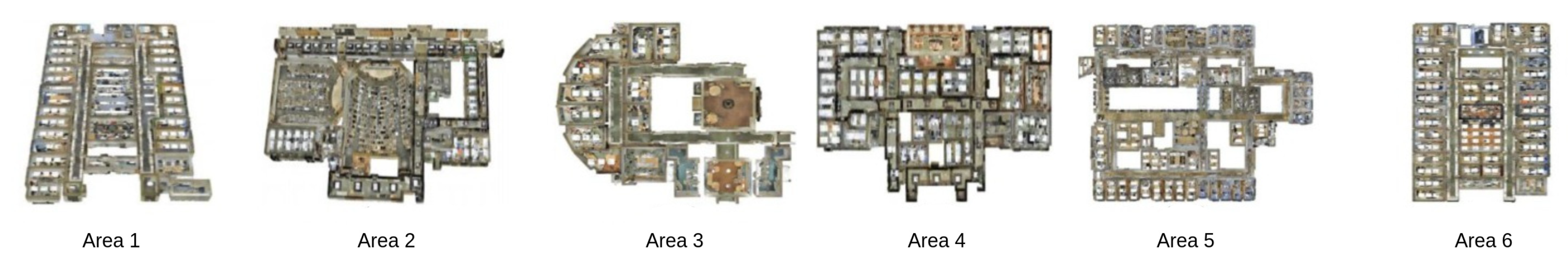
In the S3DIS dataset, we observe that in Areas 1, 3, 4, and 5 PPNet is first while KPConv is second in the test data. In Area 6 we can see that KSConv surpasses PPNet with a I m I o U score equal to 56.32 against 55.87. It is worth mentioning, that in the hardest to segment Area, Area 2, RSConv is the winner with I m I o U = 47.34 , while KPConv takes the second place with an I m I o U = 45.38 . Similarly, as in the ShapeNet-part dataset, PPNet has the highest performance in the training set in all Areas. However, by observing some poor performance cases in the test set, for example in Area 3 or Area 2, we may have overfitting issues or these Areas are hard to learn.
To analyze in-depth the segmentation behavior of the models, in Table 5a,b, we present in-depth results with ShapeNet-part and S3DIS datasets, respectively.
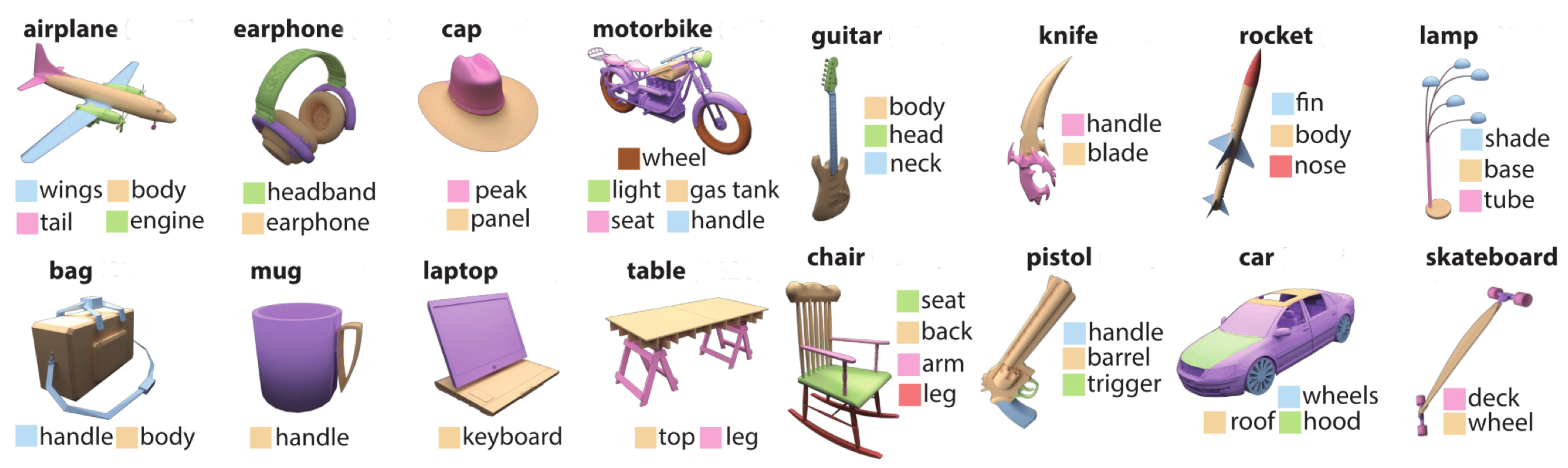
Regarding the results with ShapeNet-part, we report the segmentation accuracy per class ( C m I o U ) in the epoch where the best C m I o U is recorded for each model. It seems that all the models perform better in different classes of point cloud objects. By observing the table, we can identify that there is no perfect rule for dividing the models according to their accuracy result in each class. For instance, RSConv outperforms the other models in classes Airplane and Bag but is third or fourth in ranking in other classes such as Car or Chair. Additionally, PointNet seems to deal great with Laptop and Table labeled point clouds, but can not deal effectively with the majority of the others. In addition, it is interesting that, for example, in class Cap with 39 samples PointNet++ is the winner, while on Rocket with 46 samples the winner is PPNet and in Bag with 54 samples the winner is RSConv.
Regarding the results with S3DIS, we report the best achieved I m I o U per Area. We can see that KPConv, PPNet, and RSConv are ahead of PointNet and PointNet++ in all S3DIS Areas. We can not decide on an all-around winning model for all the Areas, as PPNet is first in Areas 1, 3, 4, and 5, but in Area 2 and Area 6 the winners are RSConv and KPConv, respectively. Thus, we highlight the Observation 1.
Observation 1.
In terms of accuracy, there is not a clearly winning model in all classes of point cloud objects in the ShapeNet-part. Additionally, it seems that there is not a clear winner in classes where the point cloud samples are limited. The worst model is PointNet, which incorporates only Rotation and Permutation invariance properties. The same insights are also observed in scene segmentation (S3DIS dataset), as there is not an absolute winner in all Areas and PointNet is the least accurate model. Finally, in both segmentation tasks, Convolution-based models obtain better results, both in training and testing.

4.3.2. Efficiency

In this section, we explore the segmentation efficiency of the selected models by analyzing the results in Table 6.
In Table 6, we display (i) the time spent (in decimal hours) to complete the whole learning process of training, validation, and testing as t t o t a l ( h ) , (ii) the time spent to achieve the best performance in relation to C m I o U and I m I o U metrics in the test data as C m I o U t i m e ( h ) b e s t , I m I o U t i m e ( h ) b e s t respectively and (iii) the number of epoch ( n e p o c h ) that corresponds to the exact time measurement. Additionally, we display (iv) the average GPU memory allocation in percentage in the whole learning process as G P U m e m . Please note that the preliminaries of the aforementioned metrics are detailed in Section 3.2.2. In S3DIS Areas, we report only the I m I o U as the C m I o U does not apply, as stated earlier.
Regarding the results in ShapeNet-part, an interesting observation is that PointNet++ is the fastest neural network with a total run time ( t t o t a l ) of 4.55 h, while being the second best in accuracy, as shown in Table 4. It also achieves its peak performance in test data faster than all its competitors, i.e., I m I o U t i m e ( h ) b e s t = 2.03 and C m I o U t i m e ( h ) b e s t = 3.36 h. RSConv and PointNet are second in I m I o U t i m e ( h ) b e s t and C m I o U t i m e ( h ) b e s t respectively. Additionally, KPConv uses the least amount of epochs to achieve the best I m I o U value in test data, i.e., n e p o c h s = 53 . Regarding the best score in C m I o U , PointNet++ uses n e p o c h s = 146 while PPNet follows with an almost identical number of epochs to achieve its best C m I o U score, n e p o c h s = 151 .
In terms of average GPU memory usage, PointNet finishes in the first place with 33.7% although the second one, PointNet++, has approximately the same GPU memory usage with a value of 36.3%. Additionally, PPNet utilizes 89% of total GPU memory while needing about 29.28 h of time for its computations, appearing to be the least efficient in terms of memory and time spent. It is worth noticing that the differences in time efficiency across the models are great, wherein on one hand we observe PointNet and PointNet++ models having t t o t a l = 5.55 and t t o t a l = 4.55 and on the other hand KPConv and PPNet having t t o t a l = 23.01 and t t o t a l = 29.28 respectively. Similarly, in average GPU memory allocation, we notice PointNet and PointNet++ models having G P U m e m = 33.7 and G P U m e m = 36.3 , and on the other hand KPConv and PPNet having G P U m e m = 60.4 and G P U m e m = 89 respectively.
Regarding the results in S3DIS Areas, we observe that PointNet++ is the fastest neural network in ( t t o t a l ), in all Areas of S3DIS, similarly as in ShapeNet-part case. However, in Area 1, PointNet achieves its peak performance I m I o U t i m e ( h ) b e s t = 2.80 faster than the others. It is noteworthy that in Area 2, RSConv not only achieves the best accuracy of I m I o U = 47.34 (Table 4) but also is faster than the other models in I m I o U t i m e ( h ) b e s t = 1.17 . Regarding the average GPU memory usage, PointNet is the winner in almost all Areas except Area 2 where PointNet++ is first. It is clear that both PointNet and PointNet++ use fewer memory resources than the others, while PPNet requires the most memory resources almost in all Areas. These remarks lead us to Observation 2.
Observation 2.
Time and memory efficiency varies greatly across different models. There is not a clearly winning model concerning efficiency in time and memory allocation. Additionally, it seems that neural networks that utilize Point-wise MLP-based operations are the ones that have the lowest time and GPU memory consumption.

4.3.3. Robustness

In this section, we analyze the results presented in Table 5 and Table 7 to investigate the segmentation robustness of the selected models.
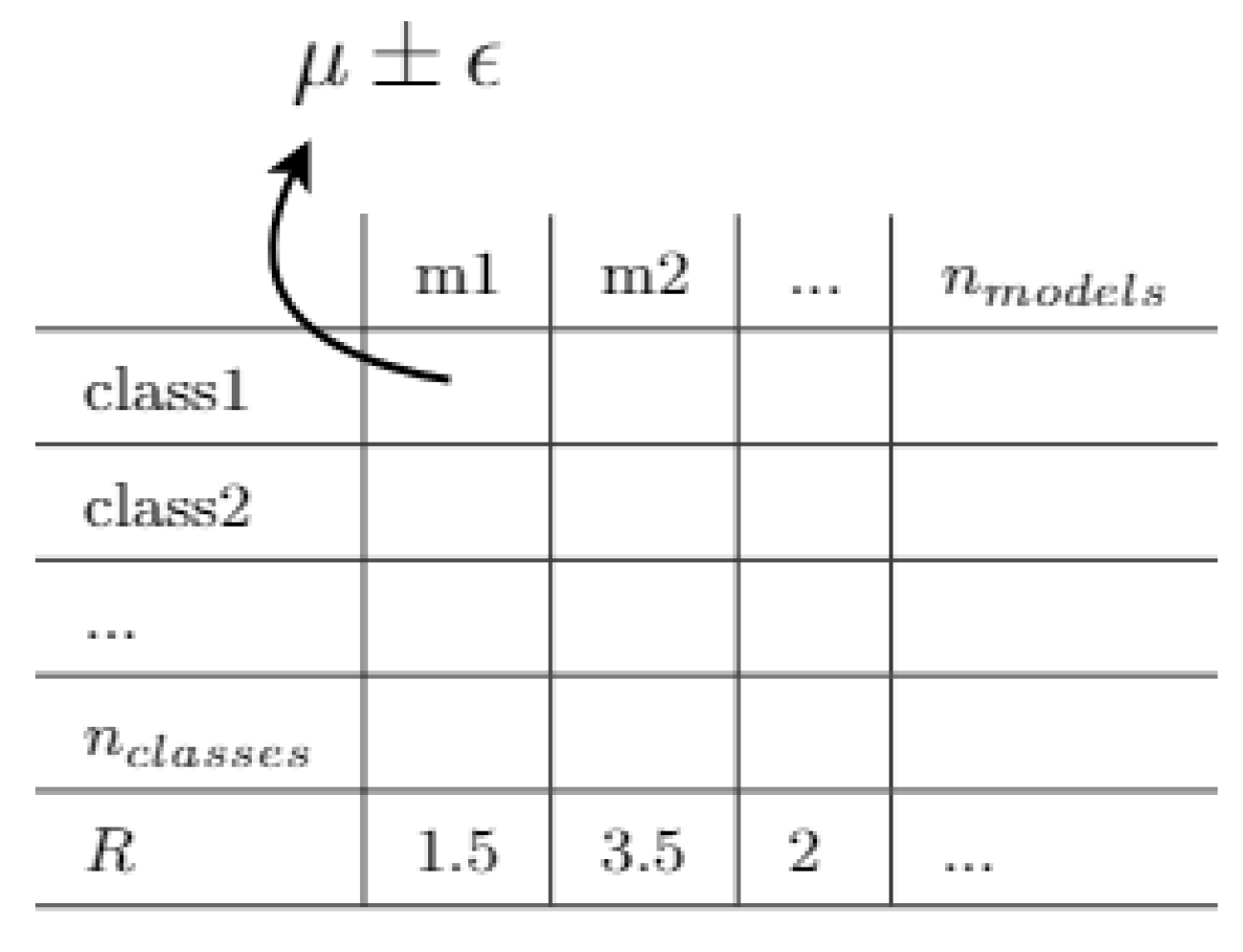
In order to further clarify the robustness of each deep learning model in each class we denote the results in μ ± ϵ format. Regarding the robustness-related results in the ShapeNet-part dataset, in the last row of Table 5(a), we display the results of m I o U metric for each class that correspond to the best epoch outcome of C m I o U of each model. Additionally, we report the average accuracy obtained in each object. Such information is useful to detect the most difficult and the easiest objects to learn. In the same notion, in Table 5(b), in the results on the S3DIS dataset, we report the best achieved m I o U per Area and also the model performance averages. We also report the average per Area in order to justify the learning difficulty of each Area.
In ShapeNet-part, PPNet has the lowest error ( ϵ = 9.75 ) of the mean ( μ = 82.50 ), while the mean performance of 82.50 is almost identical to the RSConv, which achieves 82.73 with an error of ϵ = 10.44 . Please note that in the hardest classes to learn, i.e., the ones with the lowest achieved accuracy and highest error, such as "Rocket" or "Motorbike" the winning models are KPConv and RSConv respectively, both of them being based on convolutional operations.
On the other hand, in S3DIS, PPNet achieves the best average performance in all Areas, with a model average of 63.65 ± 19.94 ( % ) , while KPConv is second with an average of 62.91 ± 18.81 ( % ) . Additionally, it can be observed that the hardest Areas to learn are Areas 2, 3, and 6, as all the models achieved significantly lower segmentation accuracy than in Areas 1, 4, and 5. Similarly, as in ShapeNet-part results, the winning models in the hardest cases are based on convolutional operations. Following, we highlight another remark in Observation 3.
Observation 3.
In the "hardest" to learn classes (part segmentation) or areas (scene segmentation) the winning models are the Convolution-based ones that incorporate Local Aggregation operations focusing on the local features of the 3D point cloud. Additionally, in some classes (e.g., Earphone) in part segmentation, the Point wise MLP-based models achieve high mean accuracy but they tend to have higher errors than the others.
Furthermore, in Table 7a, in the ShapeNet-part dataset, we report the average scores of m I o U per class that are achieved by each neural network in the testing phase of all 200 epochs. It can be observed that highly accurate models in specific classes have higher error ( ϵ ) than the others. For instance, in class Cap, PointNet++ has the highest average accuracy of 84.38 however its error of the mean seems to be higher than the others ϵ = 4.59 . On the other hand, PPNet has a lower accuracy score of 81.74 but the error ( ϵ = 2.14 ) is approximately half the one of PointNet++.
Regarding the S3DIS results in Table 7b, we report the average scores of m I o U in all six Areas, similarly as in ShapeNet-part results. In Area 2, RSConv has the best mean accuracy and also the lowest error ( 43.21 ± 2.89 ). KPConv has the best segmentation accuracy in Area 6, but its error is higher than the others. Moreover, PPNet achieves the best mean segmentation accuracy in Areas 1, 3, 4, and 5, but its error of the mean in some cases, such as Area 4 is higher than the one in KPConv or RSConv.
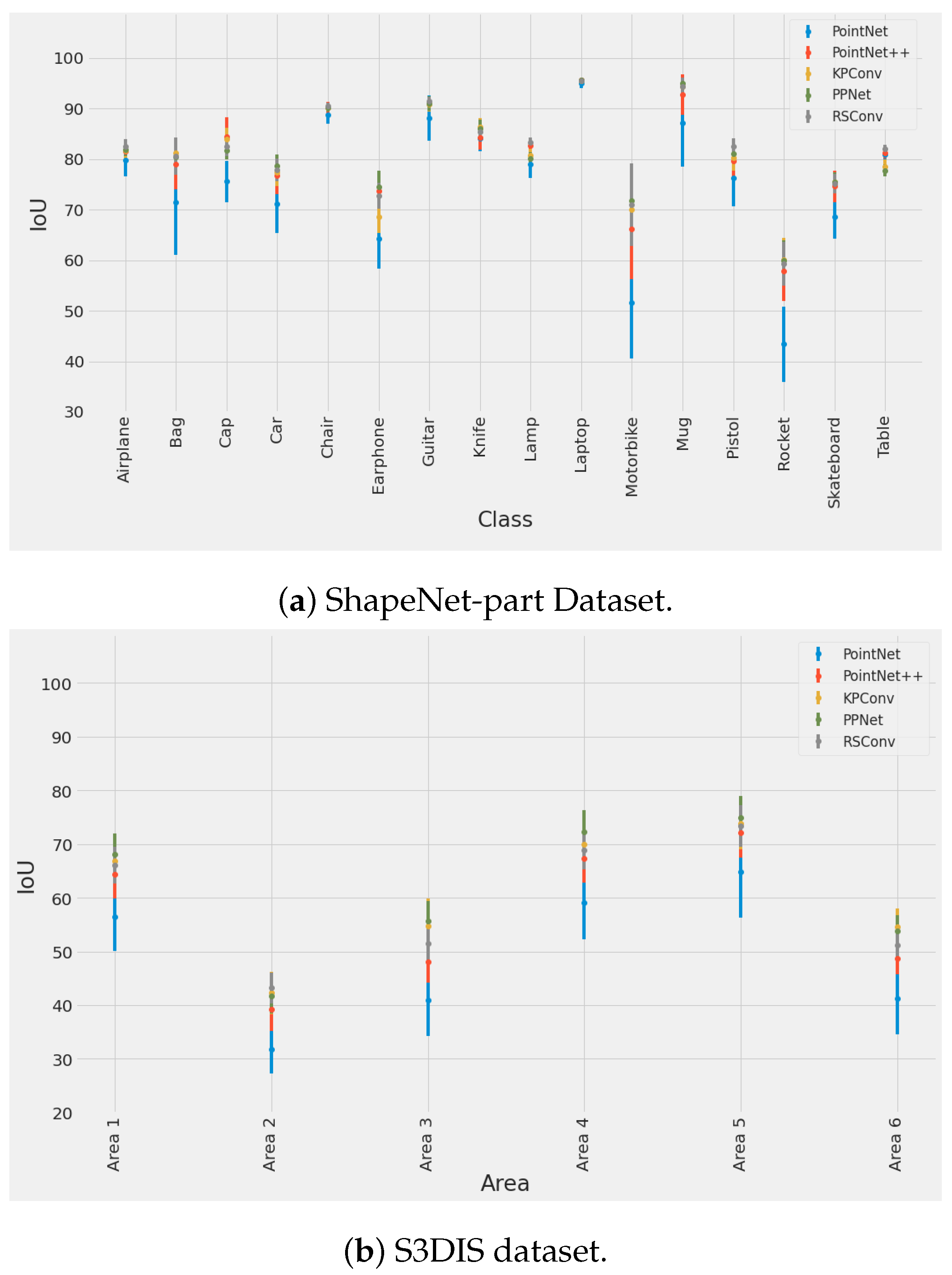
Moreover, we graphically represent the μ ± ϵ of I o U in each class of ShapeNet-part and in each Area of S3DIS in all testing epochs in Figure 4. In ShapeNet-part, the most accurate method, RSConv, shows also greater robustness than the most efficient PointNet++ model. It is interesting how the models perform in "ill" classes such as the Motorbike and Rocket. In such classes, we observe great differences among the models’ performance, although PPNet, KPConv, and RSConv achieve approximately the same segmentation accuracy and robustness. This can be also justified by Table 7, where in Rocket class the former three achieve approximately 60 ± 7 of m I o U . On the other hand, in the same class of Rocket, PointNet and PointNet++ seem to be worse with the first one being the worst reporting a 43.40 ± 17.26 .
In S3DIS, PointNet appears to be the least accurate model since it has the lowest segmentation accuracy and its error is the highest. Observing the error bars, we can say that in some occasions, such as in Area 5, the error is more than twice as high as in other models. Furthermore, we observe that the best model, PPNet, shows also good robustness. In Area 3, we see a great range of accuracy values of all the models combined ranging from approximately 35% to 60%. We can also visually identify that Areas 2, 3, and 6 are hard Areas to learn.
In addition, in order to provide a rigorous statistical evaluation in terms of per-class robustness in test data, first we use the Friedman statistical test [40], as described in Section 3.2.3. We apply the Friedman test in our experimental setup, where in the case of ShapeNet-part we have N = 16 data classes and n m o d e l s = 5 different deep learning models, and in the case of S3DIS, we have N = 6 (Areas) and n m o d e l s = 5 .
Regarding the ShapeNet-part case, the Friedman test statistic F F follows the F distribution with ( 5 1 ) = 4 and ( 5 1 ) · ( 16 1 ) = 60 degrees of freedom. The calculated Friedman test statistic is equal to F F = 14.77 , according to Equations (6) and (7). Hence, at an α = 0.05 of statistical significance, the critical value is 2.52. Next, we observe that 14.77 > 2.52 , so we have enough evidence to reject the null hypothesis H 0 , as described in Section 3.2.3. Alternatively, at an alpha level of statistical significance α = 0.05 the p v a l u e = 0 , implies that we can reject the null hypothesis. Table 7 shows the ranking of models according to the aforementioned test.
Regarding the S3DIS case, the Friedman test statistic F F follows the F distribution with ( 5 1 ) = 4 and ( 5 1 ) · ( 6 1 ) = 20 degrees of freedom. The Friedman test statistic is equal to F F = 34.09 . At an α = 0.05 of statistical significance, the critical value is 2.86 and by observing that 34.09 > 2.86 , we can safely reject the null hypothesis H 0 .
Once we have successfully rejected the null hypothesis, the Nemenyi test [40] is applied to check the presence of statistically significant differences among the models. Recall that the two models are statistically significant if their corresponding average ranks differ by at least the critical difference value ( C D ), described in Section 3.2.3. In the case of ShapeNet-part, the critical value of the two-tailed Nemenyi test (Equation (8)) that corresponds to 95% statistical significance, i.e., α = 0.05 , having n m o d e l s = 5 and N = 16 is equal to q 0.05 = 2.728 . Thus, the calculated critical difference value is C D = 1.525 and for any two pairs of models whose rank difference is higher than C D = 1.525 , we can infer with a statistical confidence of 95% that a significant difference exists among them.
In the case of S3DIS, the aforementioned critical value at an α = 0.05 while n m o d e l s = 5 and N = 6 is equal to q 0.05 = 2.728 . The calculated critical difference value is C D = 2.49 and we can infer with a statistical confidence of 95% that a significant difference exists among them.
Figure 5 portrays the Nemenyi statistical test of models. In the graph, the bullets represent the mean ranks of each model and the vertical lines indicate the critical difference. Hence, to clarify, the two methods are significantly different if their lines are not overlapping. In ShapeNet-part results, the RSConv model seems to be the winner across all models although, statistically, we can only say that the PointNet model is significantly worst that its competitors. Additionally, PPNet, KPConv, and RSConv perform almost equally according to the Nemenyi test.
By observing the Nemenyi test of S3DIS in Figure 5b, although the PPNet model appears to be the winning model, we can only justify with statistical significance that PointNet is the worst model and PPNet is better than PointNet and PointNet++ models. Having analyzed our results, we report our Observation 4.
Observation 4.
Apart from accuracy and efficiency, robustness is also a crucial concern for effective model performance evaluation. There is a great variety of different errors of the mean (ϵ) m I o U values and a global robustness comparison rule among the models can not be easily identified. Basically, Convolution-based models that incorporate Adaptive Weight-based or Position Pooling aggregation operators seem to be the winners in the statistical ranking, i.e., RSConv in part segmentation (ShapeNet-part) and PPNet in scene segmentation (S3DIS).

4.3.4. Generalized Metrics

In this section, we provide insights into the generalized performance of the utilized segmentation models by analyzing the results in Table 8.
In Table 8, we evaluate the models concerning the proposed generalized metrics (see Section 3.2.4). We display three different cases that may represent the needs of the final user. Please remind that we use the following parameter rules in the Equations (9) and (10): α 2 = α 3 = α 4 = 1 α 1 3 and β 2 = β 3 = β 4 = 1 β 1 3 to promote accurate models but also balanced in terms of efficiency and robustness by assigning equal weights to the efficiency and robustness terms of the Equations.
In the first case of ShapeNet-part results, we select values of α 1 = 0.2 and β 1 = 0.2 , which indicate that the model evaluation process is biased towards the efficiency and robustness of the models. PointNet++ is first in F C m I o U R with a value of 0.88, while RSConv is second with a value of 0.81. In F I m I o U R , PointNet++ is first again with a value of 0.82, while RSConv is second with a value of 0.81. In the generalized metric F g e n e r a l R , we observe similar behavior as PointNet++ is the winner. In the second case, where α 1 = 0.5 and β 1 = 0.5 , we portray a balanced approach, giving the same weight in segmentation accuracy, efficiency, and robustness of each model. In this case, RSConv is first in F I m I o U R with a value of 0.88, while PointNet++ obtains the best value in F C m I o U R with 0.90. Additionally, RSConv outperforms its competitors in the F g e n e r a l R metric. Finally, the third case, where α 1 = 0.9 and β 1 = 0.9 , displays a segmentation accuracy biased model selection process. Here, RSConv is the winner in all three metrics.
Please note that in all of our portrayed scenarios we use α 1 = β 1 because we basically want the models to be evaluated in their ability to produce uniformly good results not only in all point cloud instances but also in all classes. As explained in Section 3.2.1, in multi-class 3D point cloud segmentation task, we seek a model that has equally high C m I o U and I m I o U ( C m I o U I m I o U ).
Regarding the generalized metrics in S3DIS, we select the same values of α 1 and β 1 in the same scenarios in order to uniformly analyze the models. However, the metrics related to C m I o U can not be applied in this dataset. As a result, we compute only the F I m I o U R in all the scenarios. In the first scenario of α 1 = 0.2 and β 1 = 0.2 , we observe approximately the same behavior in all Areas, as PointNet++ achieves the best result. In Areas 2 and 5 RSConv is second, while in Areas 1, 3, and 6 KPConv is second. In Area 4, we have a tie between RSConv and KPConv with F I m I o U R = 0.65 . In the balanced scenario where α 1 = 0.5 and β 1 = 0.5 , in all Areas, the KPConv model is first, except Area 2, where RSConv is the winner. In Areas 1, 3 and 6 PPNet is second with values of 0.67, 0.67, and 0.65 respectively. In the last scenario, we can visually identify three performance clusters, the first one includes Areas 1, 4, and 5, where we observe similar behavior of the models as PPNet is first with F I m I o U R = 0.93 while KPConv achieves the second best values. The second cluster includes Areas 3 and 6 where KPConv and PPNet have the first and second-best scores respectively. Finally, the third performance cluster includes Area 2, where interestingly RSConv and KPConv are the two best ones. It is worth noticing that Area 2 is the “hardest” Area to learn and RSConv is the winner in both balanced and accuracy-biased evaluation scenarios. Additionally, in all scenarios of all Areas of the S3DIS dataset, the fundamental architecture PointNet holds the last position which is clearly indicating that advances have been made in the trade-off of models between accuracy, efficiency, and robustness. The analysis of the results yields Observation 5.
Observation 5.
The deployment of generalized performance evaluation metrics facilitates model selection to a great extent. Such metrics are able to easily highlight the differences among models concerning accuracy, efficiency, and robustness. It is interesting that in all selected scenarios of α 1 and β 1 values, in part segmentation, the winning models (PointNet++ and RSConv) are the ones that incorporate all the invariance properties (either weak or strong), namely Rotation, Permutation, Size and Density. In scene segmentation, utilizing Convolution-based models with Local Aggregation operators accompanied by an assortment of invariance properties (either weak or strong) is important. It seems that it is advantageous to combine invariance properties, allowing the network to select the invariance it needs.

4.3.5. Relation between Design and Experimental Properties

To sum up, in this section, we emphasize the relation between the design and experimental properties of the selected models in order to pave the way toward an effective 3D point cloud segmentation model selection. We present our results in Table 9, where the ⋆ in design properties denotes the models that utilize this property. Concerning invariance properties, and specifically in transformation-related ones (rotation, size, density), we assign ⋆ to the models that according to the literature are highly robust to such transformations, or ▿ to the models where their invariance to transformations is considered weak. In experimental properties, the numbering (1, 2) distinguishes the models that achieve the two highest scores in each property, i.e., the two best ones. Please note that in case of a tie both models are getting the same number of rankings.
By focusing the learning process on the local features of the point cloud object, using Local Aggregation operators as described in Section 3.1, we expect a model to have higher accuracy and greater robustness than a model that uses only Global Aggregation operators, but less time and memory efficiency, because of the use of a greater amount of computations. Indeed, we observe that focusing on the Global Features of a point cloud is closely related to time efficiency and GPU-memory efficiency in both part segmentation and scene segmentation, e.g., PointNet’s performance, but there is a lack of segmentation accuracy and robustness. By design, models that focus on the local features of a point cloud object capture better the geometrical topology of the points, leading to higher segmentation accuracy. For instance, RSConv focuses on the Local Features of a point cloud and captures well the geometrical topology of its points, as explained in Section 3.3, resulting in a high segmentation accuracy value, in both part segmentation and scene segmentation, as shown in Table 4 and Table 5. High performance in accuracy is also observed in PPNet and KPConv models, especially in scene segmentation. However, in part segmentation, we do not observe this behavior of RSConv in all classes of the ShapeNet-part dataset, or in classes where the point cloud samples are limited, as detailed in Observation 1. Additionally, we observe that the worst model in terms of accuracy in both part segmentation and scene segmentation, PointNet, uses only the Rotation and Permutation invariance properties and focuses on the Global Features of the input point clouds.
Convolutional operations often produce more accurate results although there are cases where Point-wise MLPs outperform them. However, Point-wise MLP-based models use shared MLP units to extract point features, which are efficient and if they are accompanied by random point sampling can be highly efficient in terms of memory and computations [9,47]. Convolution-based models, while, generally, being inefficient in terms of memory and time compared to the Point-wise MLP-based models, try to improve efficiency by splitting the convolution into multiple smaller highly efficient computations, such as matrix multiplications paired with low dimension convolutions [9]. In this work, we justify such behavior of the Convolutional-based models compared to the Point-wise MLP-based ones, as depicted in Table 9. Thus, convolutions do not correspond to time or memory efficiency and the Point-wise MLP-based models appear to be the ones that have the lowest time and GPU memory consumption on average, as explained in Observation 2.
Moreover, in the "hardest" to learn classes in part segmentation or areas in scene segmentation the winning models are the Convolution-based ones by focusing on the Local Features of the point cloud, as stated in Observation 3. Additionally, in some classes (Earphone) in part segmentation Point-wise MLP-based models can achieve high mean accuracy but they tend to have higher errors than the others.
In terms of robustness, Convolution-based neural networks that incorporate Adaptive Weight-based or Position Pooling aggregation appear to be the winners in robustness statistical ranking, while Pseudo Grid operations are following in most of the cases, as shown in Observation 4. Nevertheless, it is worth noticing that paying attention in the learning process on the local features of the point cloud using either Convolution-based or Point-wise MLP-based model often leads to greater accuracy and robustness, while greatly capturing the points topology, as shown in Table 9. Summarizing, the best results in accuracy and robustness in part segmentation and scene segmentation are recorded in models that focus on the local features of the point cloud while being Convolution-based and using Adaptive Weight-based or Position Pooling local aggregation operators.
Additionally, in Table 9, we detail the number of parameters of each model. We observe that the low number of parameters is related to efficiency but also to segmentation accuracy and robustness. Thus, the correct utilization of parameters and the architectural design of the network plays a significant role. For instance, PointNet++ and RSConv use approximately 1.4 and 3.4 million parameters respectively, while being two of the best in segmentation accuracy and robustness ranking in part segmentation. However, in scene segmentation tasks it seems that the high number of parameters is strongly correlated with high accuracy and robustness but not efficiency.
Finally, the use of generalized experimental metrics aids the interpretation of all these crucial evaluation dimensions, i.e., accuracy, efficiency, robustness. Additionally, it emphasizes the trade-off among them across various models and their design properties. For example, in a balanced model evaluation scenario among accuracy, efficiency and robustness ( α 1 = β 1 = 0.5 ), the winning models in F C m I o U R , F I m I o U R and F g e n e r a l R are the ones that are highly accurate, efficient and robust, as shown in Table 9, and, clearly highlighted in Observation 5.
Some further remarks in part segmentation, i.e., ShapeNet-part data, could be that high scores in the aforementioned experimental properties correspond to models (PointNet++ and RSConv) that mainly (i) focus on the Local Features of the point cloud and have the ability to capture the topology of the points, (ii) incorporate all the invariance properties (either weak or strong invariance), namely Rotation, Permutation, Size and Density, and (iii) use a low amount of parameters compared to others, although they come from two distinct families of deep learning architectures. For instance, PointNet++ is mainly a Point-wise MLP-based model and RSConv is a Convolution-based neural network that uses Adaptive Weight-based local aggregation operations.
In addition, further remarks in scene segmentation, i.e., S3DIS data, could be that high F I m I o U R scores correspond to models that (i) focus on the Local Features of the point cloud and (ii) incorporate the majority of invariance properties. It seems that it is advantageous to combine invariance properties, allowing the network to select the invariance it needs. Additionally, all the best models in scene segmentation utilize convolutional operations and use Pseudo Grid or Adaptive Weight or Position Pooling local aggregation type. Without the loss of generality, we can say that local aggregation operators, when properly calibrated, may yield comparable performance, as shown in [14].

5. Discussion & Limitations

Our experimental findings reveal certain differences compared to the current literature. The majority of the studies show only the best-achieved accuracy of the models [9]. Instead, we not only show the best-achieved accuracy but also show the average and the standard deviation (as a percentage error of the mean) of the measurements. It is important to show experimental results in a format of μ ± ϵ , in order to justify rigorous evaluation, as it is normal in different runs to achieve slightly different "best" results. Additionally, while Zhang et al. [27] show that the forward time of PointNet is less than PointNet++’s time, we found out that the total run time of PointNet++ is way less than PointNet’s time. This can be justified to a certain extent by the fact that PointNet++ utilizes approximately 2.5 times fewer parameters than PointNet, even though it is a more complex structure than PointNet.
Regarding the limitations of this study, first, as there is a plethora of new neural networks, we choose to investigate the widely used and most characteristic ones. For instance, we do not include graph neural networks, although they are highly accurate in downstream tasks [48,49]. Thus, an all-around performance evaluation of graph-based neural networks in 3D point cloud segmentation will be addressed in future research. Second, although, we conduct our experiments in part segmentation and indoor segmentation tasks, it is interesting to explore also outdoor segmentation datasets, e.g., Semantic3D [50]. Third, in this study, we assign the invariance properties to the models from the current literature.
To open the discussion for future research, we include our further findings concerning invariance properties. In fact, permutation invariance can be incorporated quite easily into a point-based neural network, for example, by using symmetric pooling operations [11,12]. On the other hand, size, density, and rotation transformations are properties that should be rigorously evaluated. Strict invariance is tough to achieve and if so it needs to be mathematically proven. The term "strict" denotes the situation in which the equality in Equation (1) holds. Thus, in this manuscript, we refer to transformation invariant properties denoting the robustness (strong or weak) of a model to input size, scale, density changes, and arbitrary rotations, and we utilize the terms strong and weak invariance, as explained in Section 3.1. By no means, does Table 9 show strict transformation invariance properties of the models. For instance, the majority of the networks are not strictly invariant to arbitrary rotations [51], as such invariance property is often overlooked [52]. While data augmentation techniques can be used to enhance the model’s robustness to rotations in specific datasets [53], the projection of the point clouds to a high dimensional canonical space [54] or rotation-invariant convolutions [52] are two approaches that seem capable of achieving strict rotation invariance. Moreover, size invariance is also relative and strongly depends on the amount of sizing/scaling [55]. For these reasons, we have considered that the validation of the invariance properties deserves special attention and will be addressed in depth in future research.

6. Conclusions

The majority of segmentation models on 3D point clouds focus on segmentation accuracy, especially on m I o U and variants of it, C m I o U and I m I o U . However, there is little attention on analyzing efficiency, robustness, and other potential evaluation dimensions in relation to the models’ design properties. Consequently, there is an imperative need in the literature for a deep and fine-graded analysis of segmentation models on 3D point cloud objects in order to be useful in practice in part segmentation and scene segmentation tasks.
This article presents experimental findings and aims to deeply analyze segmentation models on 3D point clouds in different performance dimensions, namely accuracy, efficiency, and robustness, and relate them with the models’ inner design characteristics. Specifically, we study the inner design and experimental properties of five representative neural networks, PointNet, PointNet++, KPConv, PPNet, and RSConv, and evaluate them in widely used segmentation datasets, namely ShapeNet-part (part segmentation) and S3DIS (scene segmentation).
Our main results relate the design properties of the models with significant experimental properties, aiming to find a correspondence between them. This particular information is crucial for designing novel neural network models and is also useful for any individual applying the current state-of-the-art models. It also facilitates the decision-making of model selection from the wide range of existing models.
We show that Convolution-based models that incorporate local aggregation operations obtain better results in both part and scene segmentation than the Point-wise MLP-based ones, and they also achieve superior performance in the “hardest” classes to learn. However, Point-wise MLP-based models have the lowest time and GPU memory consumption. Additionally, Convolution-based models that incorporate Adaptive Weight-based or Position Pooling local aggregation operators are the most robust ones according to the employed Friedman–Nemenyi statistical ranking. By further relating the model invariance properties with the proposed generalized metrics F C m I o U R , F I m I o U R and F g e n e r a l R , in both part and scene segmentation, the winning models are the ones that incorporate all the invariance properties (either weak or strong), namely Rotation, Permutation, Size, and Density. It seems that it is advantageous to combine invariance properties, allowing the network to select the invariance it needs. Finally, in a balanced model evaluation scenario among accuracy, efficiency and robustness, the winning models in the proposed generalized metrics are the ones that are highly accurate, efficient and robust.
To sum up, an all-around performance evaluation of 3D point cloud segmentation models should be the de facto standard. The new upcoming neural network models in the field should not only be evaluated on their accuracy but also their efficiency and robustness. Additionally, local aggregation operator types should be studied further to better assess their efficacy in different network architectures. Finally, as we could not find extensive research on invariance properties, we believe that the experimental evaluation and validation of invariance properties in 3D point cloud learning is a research area with high potential to explore.

Author Contributions

Conceptualization, T.Z, M.S. and A.P.; methodology, T.Z, M.S. and A.P.; software, T.Z.; validation, T.Z, M.S. and A.P.; formal analysis, T.Z, M.S. and A.P.; writing—original draft preparation, T.Z.; writing—review and editing, T.Z, M.S. and A.P.; supervision, M.S. and A.P.; project administration, M.S. and A.P.; funding acquisition, M.S. and A.P. All authors have read and agreed to the published version of the manuscript.

Funding

This project has received funding from the European Union’s Horizon 2020 research and innovation programme under the Marie Skłodowska-Curie grant agreement No. 860843.

Data Availability Statement

The data used in our study are publicly available datasets. The Stanford 3D Indoor Scene Dataset (S3DIS) is available at this link: http://buildingparser.stanford.edu/dataset.html (accessed on 21 September 2022). Also, the ShapeNet-part dataset can be found in this link: https://shapenet.org/ (accessed on 21 September 2022).

Conflicts of Interest

The authors declare that they have no known competing financial interests or personal relationships that could have appeared to influence the work reported in this paper.

References

  1. Zhou, W.; Berrio, J.S.; Worrall, S.; Nebot, E. Automated Evaluation of Semantic Segmentation Robustness for Autonomous Driving. IEEE Trans. Intell. Transp. Syst. 2020, 21, 1951–1963. [Google Scholar] [CrossRef] [Green Version]
  2. Cui, Y.; Chen, R.; Chu, W.; Chen, L.; Tian, D.; Li, Y.; Cao, D. Deep Learning for Image and Point Cloud Fusion in Autonomous Driving: A Review. IEEE Trans. Intell. Transp. Syst. 2022, 23, 722–739. [Google Scholar] [CrossRef]
  3. Bello, S.A.; Yu, S.; Wang, C.; Adam, J.M.; Li, J. Review: Deep Learning on 3D Point Clouds. Remote Sens. 2020, 12, 1729. [Google Scholar] [CrossRef]
  4. Cai, Y.; Fan, L.; Atkinson, P.M.; Zhang, C. Semantic Segmentation of Terrestrial Laser Scanning Point Clouds Using Locally Enhanced Image-Based Geometric Representations. IEEE Trans. Geosci. Remote. Sens. 2022, 60, 5702815. [Google Scholar] [CrossRef]
  5. Poux, F.; Mattes, C.; Selman, Z.; Kobbelt, L. Automatic region-growing system for the segmentation of large point clouds. Autom. Constr. 2022, 138, 104250. [Google Scholar] [CrossRef]
  6. Wang, Q.; Tan, Y.; Mei, Z. Computational Methods of Acquisition and Processing of 3D Point Cloud Data for Construction Applications. Arch. Comput. Methods Eng. 2020, 27, 479–499. [Google Scholar] [CrossRef]
  7. Grilli, E.; Remondino, F. Classification of 3D Digital Heritage. Remote Sens. 2019, 11, 847. [Google Scholar] [CrossRef] [Green Version]
  8. Saiti, E.; Theoharis, T. Multimodal registration across 3D point clouds and CT-volumes. Comput. Graph. 2022, 106, 259–266. [Google Scholar] [CrossRef]
  9. Guo, Y.; Wang, H.; Hu, Q.; Liu, H.; Liu, L.; Bennamoun, M. Deep Learning for 3D Point Clouds: A Survey. IEEE Trans. Pattern Anal. Mach. Intell. 2021, 43, 4338–4364. [Google Scholar] [CrossRef]
  10. Nguyen, A.; Le, B. 3D point cloud segmentation: A survey. In Proceedings of the 6th IEEE Conference on Robotics, Automation and Mechatronics (RAM), Manila, Philippines, 12–15 November 2013; pp. 225–230. [Google Scholar] [CrossRef]
  11. Qi, C.R.; Su, H.; Mo, K.; Guibas, L.J. PointNet: Deep learning on point sets for 3D classification and segmentation. In Proceedings of the 30th IEEE Conference on Computer Vision and Pattern Recognition (CVPR), Honolulu, HI, USA, 21–26 July 2017; pp. 77–85. [Google Scholar] [CrossRef] [Green Version]
  12. Qi, C.R.; Yi, L.; Su, H.; Guibas, L.J.; Li, C.R.Q.; Hao, Y.; Leonidas, S.; Guibas, J. PointNet++: Deep hierarchical feature learning on point sets in a metric space. In Proceedings of the Advances in Neural Information Processing Systems. Neural Information Processing Systems Foundation, Long Beach, CA, USA, 4–9 December 2017; pp. 5100–5109. [Google Scholar] [CrossRef]
  13. Thomas, H.; Qi, C.R.; Deschaud, J.E.; Marcotegui, B.; Goulette, F.; Guibas, L. KPConv: Flexible and deformable convolution for point clouds. In Proceedings of the IEEE International Conference on Computer Vision (ICCV), Seoul, Republic of Korea, 27 October–2 November 2019; pp. 6410–6419. [Google Scholar] [CrossRef] [Green Version]
  14. Liu, Z.; Hu, H.; Cao, Y.; Zhang, Z.; Tong, X. A Closer Look at Local Aggregation Operators in Point Cloud Analysis. In Proceedings of the European Conference on Computer Vision (ECCV), Glasgow, UK, 23–28 August 2020; Volume 12368. LNCS. [Google Scholar] [CrossRef]
  15. Liu, Y.; Fan, B.; Xiang, S.; Pan, C. Relation-Shape Convolutional Neural Network for Point Cloud Analysis. In Proceedings of the 2019 IEEE/CVF Conference on Computer Vision and Pattern Recognition (CVPR), Long Beach, CA, USA, 16–20 June 2019; pp. 8887–8896. [Google Scholar] [CrossRef] [Green Version]
  16. Yi, L.; Kim, V.G.; Ceylan, D.; Shen, I.C.; Yan, M.; Su, H.; Lu, C.; Huang, Q.; Sheffer, A.; Guibas, L. A scalable active framework for region annotation in 3D shape collections. ACM Trans. Graph. 2016, 35, 1–12. [Google Scholar] [CrossRef]
  17. Armeni, I.; Sener, O.; Zamir, A.R.; Jiang, H.; Brilakis, I.; Fischer, M.; Savarese, S. 3D semantic parsing of large-scale indoor spaces. In Proceedings of the IEEE Computer Society Conference on Computer Vision and Pattern Recognition, Las Vegas, NV, USA, 27–30 June 2016; pp. 1534–1543. [Google Scholar] [CrossRef]
  18. Minaee, S.; Boykov, Y.Y.; Porikli, F.; Plaza, A.J.; Kehtarnavaz, N.; Terzopoulos, D. Image Segmentation Using Deep Learning: A Survey. IEEE Trans. Pattern Anal. Mach. Intell. 2022, 44, 3523–3542. [Google Scholar] [CrossRef] [PubMed]
  19. Akkus, Z.; Galimzianova, A.; Hoogi, A.; Rubin, D.L.; Erickson, B.J. Deep Learning for Brain MRI Segmentation: State of the Art and Future Directions. J. Digit. Imaging 2017, 30, 449–459. [Google Scholar] [CrossRef] [Green Version]
  20. Dou, Q.; Chen, H.; Yu, L.; Zhao, L.; Qin, J.; Wang, D.; Mok, V.C.; Shi, L.; Heng, P.A. Automatic Detection of Cerebral Microbleeds from MR Images via 3D Convolutional Neural Networks. IEEE Trans. Med. Imaging 2016, 35, 1182–1195. [Google Scholar] [CrossRef] [PubMed]
  21. Garcia-Garcia, A.; Orts-Escolano, S.; Oprea, S.; Villena-Martinez, V.; Martinez-Gonzalez, P.; Garcia-Rodriguez, J. A survey on deep learning techniques for image and video semantic segmentation. Appl. Soft Comput. 2018, 70, 41–65. [Google Scholar] [CrossRef]
  22. Kamann, C.; Rother, C. Benchmarking the Robustness of Semantic Segmentation Models with Respect to Common Corruptions. Int. J. Comput. Vis. 2020, 129, 462–483. [Google Scholar] [CrossRef]
  23. Kamann, C.; Rother, C. Increasing the Robustness of Semantic Segmentation Models with Painting-by-Numbers. In Proceedings of the European Conference on Computer Vision (ECCV), Glasgow, UK, 23–28 August 2020; Springer: Cham, Switzerland; Volume 12355. LNCS. [Google Scholar] [CrossRef]
  24. Isensee, F.; Jaeger, P.F.; Kohl, S.A.A.; Petersen, J.; Maier-Hein, K.H. nnU-Net: A self-configuring method for deep learning-based biomedical image segmentation. Nat. Methods 2020, 18, 203–211. [Google Scholar] [CrossRef]
  25. Weinmann, M.; Jutzi, B.; Hinz, S.; Mallet, C. Semantic point cloud interpretation based on optimal neighborhoods, relevant features and efficient classifiers. ISPRS J. Photogramm. Remote Sens. 2015, 105, 286–304. [Google Scholar] [CrossRef]
  26. Xie, Y.; Tian, J.; Zhu, X.X. Linking Points with Labels in 3D: A Review of Point Cloud Semantic Segmentation. IEEE Geosci. Remote Sens. Mag. 2020, 8, 38–59. [Google Scholar] [CrossRef] [Green Version]
  27. Zhang, J.; Zhao, X.; Chen, Z.; Lu, Z. A Review of Deep Learning-Based Semantic Segmentation for Point Cloud. IEEE Access 2019, 7, 179118–179133. [Google Scholar] [CrossRef]
  28. Chen, L.; Xu, Z.; Fu, Y.; Huang, H.; Wang, S.; Li, H. DAPnet: A Double Self-attention Convolutional Network for Point Cloud Semantic Labeling. IEEE J. Sel. Top. Appl. Earth Obs. Remote Sens. 2020, 14, 9680–9691. [Google Scholar] [CrossRef]
  29. Hegde, S.; Gangisetty, S. PIG-Net: Inception based deep learning architecture for 3D point cloud segmentation. Comput. Graph. 2021, 95, 13–22. [Google Scholar] [CrossRef]
  30. Peyghambarzadeh, S.M.; Azizmalayeri, F.; Khotanlou, H.; Salarpour, A. Point-PlaneNet: Plane kernel based convolutional neural network for point clouds analysis. Digit. Signal Process. 2020, 98, 102633. [Google Scholar] [CrossRef]
  31. Hu, Q.; Yang, B.; Khalid, S.; Xiao, W.; Trigoni, N.; Markham, A. Towards Semantic Segmentation of Urban-Scale 3D Point Clouds: A Dataset, Benchmarks and Challenges. In Proceedings of the 2021 IEEE/CVF Conference on Computer Vision and Pattern Recognition (CVPR), Nashville, TN, USA, 19–25 June 2021; pp. 4975–4985. [Google Scholar] [CrossRef]
  32. Sun, J.; Zhang, Q.; Kailkhura, B.; Yu, Z.; Xiao, C.; Mao, Z.M. Benchmarking Robustness of 3D Point Cloud Recognition Against Common Corruptions. arXiv 2022, arXiv:2201.12296. [Google Scholar] [CrossRef]
  33. Mao, J.; Wang, X.; Li, H. Interpolated convolutional networks for 3D point cloud understanding. In Proceedings of the IEEE International Conference on Computer Vision, Seoul, Republic of Korea, 27 October–2 November 2019; pp. 1578–1587. [Google Scholar] [CrossRef] [Green Version]
  34. Zhang, Z.; Hua, B.S.; Yeung, S.K. ShellNet: Efficient Point Cloud Convolutional Neural Networks Using Concentric Shells Statistics. In Proceedings of the 2019 IEEE/CVF International Conference on Computer Vision (ICCV), Seoul, Republic of Korea, 27 October–2 November 2019; pp. 1607–1616. [Google Scholar] [CrossRef] [Green Version]
  35. Tatarchenko, M.; Park, J.; Koltun, V.; Zhou, Q.Y. Tangent Convolutions for Dense Prediction in 3D. In Proceedings of the IEEE/CVF Conference on Computer Vision and Pattern Recognition, Salt Lake City, UT, USA, 18–22 June 2018; pp. 3887–3896. [Google Scholar] [CrossRef] [Green Version]
  36. Wang, S.; Suo, S.; Ma, W.C.; Pokrovsky, A.; Urtasun, R. Deep Parametric Continuous Convolutional Neural Networks. In Proceedings of the IEEE Computer Society Conference on Computer Vision and Pattern Recognition, Salt Lake City, UT, USA, 18–22 June 2018; pp. 2589–2597. [Google Scholar] [CrossRef]
  37. Wu, W.; Qi, Z.; Fuxin, L. PointCONV: Deep convolutional networks on 3D point clouds. In Proceedings of the IEEE Computer Society Conference on Computer Vision and Pattern Recognition, Long Beach, CA, USA, 15–20 June 2019; pp. 9613–9622. [Google Scholar] [CrossRef] [Green Version]
  38. Qiu, Z.; Li, Y.; Wang, Y.; Pan, Y.; Yao, T.; Mei, T. SPE-Net: Boosting Point Cloud Analysis via Rotation Robustness Enhancement. In Proceedings of the European Conference of Computer Vision (ECCV), Tel Aviv, Israel, 23–27 October 2022; Springer: Cham, Switzerland; pp. 593–609. [Google Scholar] [CrossRef]
  39. Lin, H.; Fan, B.; Liu, Y.; Yang, Y.; Pan, Z.; Shi, J.; Pan, C.; Xie, H. PointSpherical: Deep Shape Context for Point Cloud Learning in Spherical Coordinates. In Proceedings of the 2020 25th International Conference on Pattern Recognition (ICPR), Milan, Italy, 10–15 January 2021; pp. 10266–10273. [Google Scholar] [CrossRef]
  40. Demšar, J. Statistical Comparisons of Classifiers over Multiple Data Sets. J. Mach. Learn. Res. 2006, 7, 1–30. [Google Scholar] [CrossRef]
  41. Wilcox, R.R. Rank-based and nonparametric methods. In Applying Contemporary Statistical Techniques; Academic Press: Cambridge, CA, USA, 2003; pp. 557–608. [Google Scholar] [CrossRef]
  42. Zoumpekas, T.; Molina, G.; Salamó, M.; Puig, A. Benchmarking Deep Learning Models on Point Cloud Segmentation. In Artificial Intelligence Research and Development; IOS Press: Amsterdam, The Netherlands, 2021; Volume 339, pp. 335–344. [Google Scholar] [CrossRef]
  43. Chaton, T.; Chaulet, N.; Horache, S.; Landrieu, L. Torch-Points3D: A Modular Multi-Task Framework for Reproducible Deep Learning on 3D Point Clouds. In Proceedings of the 2020 International Conference on 3D Vision (3DV), Fukuoka, Japan, 25–28 November 2020; pp. 190–199. [Google Scholar] [CrossRef]
  44. Tian, F.; Jiang, Z.; Jiang, G. DNet: Dynamic Neighborhood Feature Learning in Point Cloud. Sensors 2021, 21, 2327. [Google Scholar] [CrossRef]
  45. Armeni, I.; Sax, S.; Zamir, A.R.; Savarese, S. Joint 2D-3D-Semantic Data for Indoor Scene Understanding. arXiv 2017, arXiv:1702.01105. [Google Scholar] [CrossRef]
  46. Liang, X.; Fu, Z.; Sun, C.; Hu, Y. MHIBS-Net: Multiscale hierarchical network for indoor building structure point clouds semantic segmentation. Int. J. Appl. Earth Obs. Geoinf. 2021, 102, 102449. [Google Scholar] [CrossRef]
  47. Hu, Q.; Yang, B.; Xie, L.; Rosa, S.; Guo, Y.; Wang, Z.; Trigoni, N.; Markham, A. RandLA-Net: Efficient Semantic Segmentation of Large-Scale Point Clouds. In Proceedings of the IEEE/CVF Conference on Computer Vision and Pattern Recognition, Seattle, WA, USA, 14–19 June 2020; pp. 11105–11114. [Google Scholar] [CrossRef]
  48. Lei, H.; Akhtar, N.; Mian, A. Spherical Kernel for Efficient Graph Convolution on 3D Point Clouds. IEEE Trans. Pattern Anal. Mach. Intell. 2021, 43, 3664–3680. [Google Scholar] [CrossRef] [Green Version]
  49. Landrieu, L.; Boussaha, M. Point Cloud Oversegmentation with Graph-Structured Deep Metric Learning. In Proceedings of the IEEE Computer Society Conference on Computer Vision and Pattern Recognition, Long Beach, CA, USA, 15–20 June 2019; pp. 7432–7441. [Google Scholar] [CrossRef]
  50. Hackel, T.; Savinov, N.; Ladicky, L.; Wegner, J.D.; Schindler, K.; Pollefeys, M. Semantic3D.net: A new Large-scale Point Cloud Classification Benchmark. ISPRS Ann. Photogramm. Remote. Sens. Spat. Inf. Sci. 2017, 4, 91–98. [Google Scholar] [CrossRef]
  51. Sahin, Y.H.; Mertan, A.; Unal, G. ODFNet: Using orientation distribution functions to characterize 3D point clouds. Comput. Graph. 2020, 102, 610–618. [Google Scholar] [CrossRef]
  52. Zhang, Z.; Hua, B.S.; Yeung, S.K. RIConv++: Effective Rotation Invariant Convolutions for 3D Point Clouds Deep Learning. Int. J. Comput. Vis. 2022, 130, 1228–1243. [Google Scholar] [CrossRef]
  53. Bai, X.; Luo, Z.; Zhou, L.; Fu, H.; Quan, L.; Tai, C.L. D3Feat: Joint Learning of Dense Detection and Description of 3D Local Features. In Proceedings of the IEEE Computer Society Conference on Computer Vision and Pattern Recognition, Seattle, WA, USA, 14–19 June 2020; pp. 6358–6366. [Google Scholar] [CrossRef]
  54. Fujiwara, K.; Hashimoto, T. Neural implicit embedding for point cloud analysis. In Proceedings of the IEEE Computer Society Conference on Computer Vision and Pattern Recognition, Seattle, WA, USA, 14–19 June 2020; pp. 11731–11740. [Google Scholar] [CrossRef]
  55. Lin, Z.H.; Huang, S.Y.; Wang, Y.C.F. Learning of 3D Graph Convolution Networks for Point Cloud Analysis. IEEE Trans. Pattern Anal. Mach. Intell. 2022, 44, 4212–4224. [Google Scholar] [CrossRef] [PubMed]
Figure 1. Definition of the robustness term R. Please note that m1 and m2 correspond to two different models, and class1 and class2 indicate two distinct classes. Additionally, the values in the cells of the last row are just example values.
Remotesensing 14 06049 g001
Figure 2. ShapeNet-part 3D point cloud objects [16].
Remotesensing 14 06049 g002
Figure 3. S3DIS dataset [17,45,46].
Remotesensing 14 06049 g003
Figure 4. Comparison of deep learning models in terms of m I o U over all testing epochs. The bullet in the middle of each bar denotes the mean ( μ ) and the bar shows the error interval ( ± ϵ of the mean). Figure (a) shows the results in the ShapeNet-part dataset and Figure (b) the results in S3DIS.
Remotesensing 14 06049 g004
Figure 5. Nemenyi comparison of deep learning models. The bullets in the bars represent the mean ranks of each model and the vertical lines show the critical difference in the statistical test. Figure (a) shows the results in the ShapeNet-part dataset and Figure (b) the results in S3DIS.
Remotesensing 14 06049 g005
Table 1. Summary of experimental properties.
Evaluation DimensionsExperimental Properties
Accuracy I m I o U , C m I o U
Efficiency t t o t a l , C m I o U t i m e ( h ) b e s t , I m I o U t i m e ( h ) b e s t , G P U m e m , n e p o c h
Robustnessranking based on μ ± ϵ
Generalized Performance F C m I o U R , F I m I o U R , F g e n e r a l R
Table 2. Summary of deep learning models and their design characteristics. Please note that we use certain abbreviations, i.e NN: Neural Network, Conv: Convolution, MLP: Multi-Layer Perceptron, Rot: Rotation, Per: Permutation, Dens: Density, #: number.
ModelAggregation LevelAggregation TypeNN MethodInvariance# of Parameters
PointNetGlobalPoint-wiseMLPRot, Per3.5 M
PointNet++LocalPoint-wiseMLPRot, Per, Size, Dens1.4 M
KPConvLocalPseudo GridConvRot, Per, Size, Dens14.2 M
PPNetLocalPosition PoolingConvPer, Size, Dens18.5 M
RSConvLocalAdaptive WeightConvRot, Perm, Size, Dens3.5 M
Table 3. Description of ShapeNet-part segmentation data. We denote with n the number of annotated parts. We further show the training, validation, and test splits with the total number of samples per class.
nTrainingValidationTestTotal
Aeroplane419583913412690
Bag25481476
Cap23951155
Car465981158898
Chair426583967043758
Earphone34961469
Guitar355078159787
Knife22773580392
Lamp411181432861547
Laptop23244483451
Motorbike61252651202
Mug21301638184
Pistol32093044283
Rocket34681266
Skateboard31061531152
Table338355888485271
Total5012,1371870287416,881
Table 4. Comparison of deep learning models in terms of segmentation accuracy evaluation of the learning process in 200 epochs. In table (a), we display I m I o U and C m I o U metrics (best-achieved score) on the ShapeNet-part dataset and, similarly, in the table (b) we show the m I o U (or alternatively the I m I o U ) metric on all the Areas of S3DIS dataset. We use dark grey and light grey cell colors to denote the best and the second best score per metric respectively.
(a) ShapeNet-part dataset.
DataMetricPointNetPointNet++KPConvPPNetRSConv
Training Set I m I o U V a l u e 89.8090.4591.9992.3791.53
n e p o c h 182181189174194
C m I o U V a l u e 89.8190.8591.9192.8992.39
n e p o c h 183185188179177
Validation Set I m I o U V a l u e 86.3986.8386.6186.4687.12
n e p o c h 169144544666
C m I o U V a l u e 79.8783.0882.4382.5682.82
n e p o c h 167174166174123
Test Set I m I o U V a l u e 84.2484.9384.2283.8785.47
n e p o c h 170885316771
C m I o U V a l u e 79.0382.5082.3982.5082.73
n e p o c h 178146189151194
(b) S3DIS dataset
DataMetricPointNetPointNet++KPConvPPNetRSConv
Training setAreas 2, 3, 4, 5, 6 V a l u e 93.2494.6595.6696.4696.22
n e p o c h 196198183194175
Test SetArea 1 V a l u e 60.6466.6269.2170.8968.00
n e p o c h 140166186169124
Training SetAreas 1, 3, 4, 5, 6 V a l u e 92.9194.8295.4696.5896.13
n e p o c h 196188197190185
Test SetArea 2 V a l u e 34.4142.2845.3845.2447.34
n e p o c h 13174643826
Training SetAreas 1, 2, 4, 5, 6 V a l u e 93.7895.0095.6396.5996.31
n e p o c h 196197187191196
Test SetArea 3 V a l u e 44.5250.2857.4357.5553.41
n e p o c h 18311118017580
Training SetAreas 1, 2, 3, 5, 6 V a l u e 93.1894.4595.5296.5196.09
n e p o c h 198193197175189
Test SetArea 4 V a l u e 62.4969.7372.6475.0071.98
n e p o c h 14413070136119
Training SetAreas 1, 2, 3, 4, 6 V a l u e 92.9494.3195.1996.3895.87
n e p o c h 195190194196197
Test SetArea 5 V a l u e 69.9374.9976.5177.3575.68
n e p o c h 17018515814390
Training SetAreas 1, 2, 3, 4, 5 V a l u e 93.1494.9495.6096.4696.27
n e p o c h 195194198193194
Test SetArea 6 V a l u e 45.0850.9256.3255.8752.30
n e p o c h 1744186131161
Table 5. Comparisons of deep learning models in terms of best segmentation accuracy. Please note that in the table (a) each row shows the m I o U value for each class and the last row shows the C m I o U , which is the average of all the m I o U per class across all classes for each model and the error of it in percentage values, denoted as ϵ . Also in the same format of average ± ϵ , we show the per object average and the standard error of the mean. In table (b), we show the best m I o U per Area in each row and, similarly as in table (a), the models’ and Areas’ average and their errors. We use dark grey and light grey cell colors to denote the best and the second-best score in each row.
(a) ShapeNet-part Dataset.
PointNetPointNet++KPConvPPNetRSConvObject Avg ± ϵ
Airplane82.5582.6381.9082.3683.2382.53 ± 0.58
Bag80.2281.7982.7781.3583.7381.97 ± 1.64
Cap76.0385.8383.8582.6483.4782.36 ± 4.53
Car75.9177.9979.1579.8479.0378.39 ± 1.96
Chair90.2190.5590.4690.6990.4090.46 ± 0.20
Earphone68.8079.3472.3676.6973.6574.17 ± 5.45
Guitar91.5091.2791.8791.5891.8791.62 ± 0.28
Knife87.1485.2387.2286.9585.3186.36 ± 1.17
Lamp80.9283.1180.8880.7383.9081.91 ± 1.81
Laptop95.7895.3295.5095.4895.4795.51 ± 0.18
Motorbike61.3270.9774.2774.7774.9871.26 ± 8.13
Mug91.9194.2295.9495.4095.3494.56 ± 1.70
Pistol79.7381.9981.9382.5883.9082.03 ± 1.84
Rocket46.3461.5663.5065.3461.7159.69 ± 12.76
Table81.6881.2678.8977.6581.5980.21 ± 2.29
CmIoU ± ϵ 79.03 ± 15.8282.50 ± 10.3782.39 ± 10.4282.50 ± 9.7582.73 ± 10.44
(b) S3DIS Dataset.
PointNetPointNet++KPConvPPNetRSConvArea Avg   ±   ϵ
Area 160.6466.6269.2170.8968.0067.07 ± 5.85
Area 234.4142.2845.3845.2447.3442.93 ± 11.86
Area 344.5250.2857.4357.5553.4152.64 ± 10.37
Area 462.4969.7372.6475.0071.9870.37 ± 6.80
Area 569.9374.9976.5177.3575.6874.89 ± 3.89
Area 645.0850.9256.3255.8752.3052.10 ± 8.73
Model Avg ± ϵ 52.84 ± 25.6059.14 ± 22.0562.91 ± 18.8163.65 ± 19.9461.45 ± 19.31
Table 6. Comparison of the efficiency of the utilized deep learning models in 200 epochs. Time values are shown in decimal hours (h). In table (a) we show the results utilizing the ShapeNet-part dataset and in tables (bg) we show the results in all Areas of S3DIS dataset. Please note that in S3DIS, tables (bg), the C m I o U values are missing, because such a performance metric is not applied in this dataset. We use dark grey and light grey cell colors to denote the best and the second best score per metric respectively.
(a) ShapeNet-part dataset.
Method t total ( h ) ImIoU time ( h ) best CmIoU time ( h ) best GPU mem ( % )
Value n epoch Value n epoch
PointNet5.554.771704.9917833.7
PointNet++4.552.03883.3614636.3
KPConv23.016.215321.9618960.4
PPNet29.2824.7116722.3315189.0
RSConv12.064.357111.8119455.5
(b) Area 1—S3DIS dataset.(c) Area 2—S3DIS dataset.
Method t total ( h ) ImIoU time ( h ) best GPU mem ( % ) Method t total ( h ) ImIoU time ( h ) best GPU mem ( % )
Value n epoch Value n epoch
PointNet3.982.8014031.8PointNet3.942.5913133.8
PointNet++3.372.8116632.8PointNet++3.241.207432.7
KPConv17.3416.2118646.8KPConv16.915.446453.6
PPNet22.5019.1116977.3PPNet21.574.123889.0
RSConv8.895.5412453.1RSConv8.931.172654.8
(d) Area 3—S3DIS dataset.(e) Area 4—S3DIS dataset.
Method t total ( h ) ImIoU time ( h ) best GPU mem ( % ) Method t total ( h ) ImIoU time ( h ) best GPU mem ( % )
Value n epoch Value n epoch
PointNet4.083.7518330.2PointNet4.293.1014429.8
PointNet++3.381.8911132.9PointNet++3.542.3113034.2
KPConv17.7316.0418046.4KPConv18.756.607043.0
PPNet22.5719.8517575.7PPNet24.2516.5713694.0
RSConv9.073.658052.1RSConv9.615.7511951.8
Method t total ( h ) ImIoU time ( h ) best GPU mem ( % ) Method t total ( h ) ImIoU time ( h ) best GPU mem ( % )
Value n epoch Value n epoch
PointNet4.053.4617031.3PointNet3.753.2817430.6
PointNet++3.323.0918534.1PointNet++3.230.674133.3
KPConv17.5713.9515848.6KPConv15.666.778648.3
PPNet22.3316.0514377.1PPNet20.1013.2313180.5
RSConv8.924.039053.2RSConv8.226.6516152.4
Table 7. Comparison of deep learning models in terms of m I o U per class in the whole learning procedure (averaged over 200 epochs). In table (a) we show the results in the ShapeNet-part dataset and in the table (b) we display the results in the S3DIS dataset. We use dark and light grey colors to denote the best and the second-best model. Please note that the last row of both tables, entitled "Ranking", refers to the ranking mechanism described in Section 3.2.3.
(a) ShapeNet-part dataset.
ClassPointNetPointNet++KPConvPPNetRSConv
μ ± ϵ μ ± ϵ μ ± ϵ μ ± ϵ μ ± ϵ
Airplane79.88 ± 4.1281.59 ± 2.2781.81 ± 2.2181.90 ± 1.5782.48 ± 1.82
Bag71.44 ± 14.5079.00 ± 6.2181.24 ± 3.0080.39 ± 3.7380.60 ± 4.51
Cap75.57 ± 5.4484.38 ± 4.5983.98 ± 2.6581.74 ± 2.1482.60 ± 2.50
Car71.16 ± 8.0676.81 ± 4.8777.43 ± 3.4878.65 ± 2.9177.95 ± 2.86
Chair88.71 ± 1.8890.21 ± 1.2390.19 ± 0.6990.30 ± 0.9190.50 ± 0.72
Earphone64.28 ± 9.3573.72 ± 5.4768.64 ± 4.8474.46 ± 4.4672.76 ± 3.55
Guitar88.18 ± 5.0991.05 ± 1.4490.85 ± 1.5590.97 ± 1.5991.50 ± 0.83
Knife84.07 ± 2.9684.34 ± 2.8786.42 ± 2.0686.01 ± 2.1285.45 ± 1.31
Lamp78.99 ± 3.3882.68 ± 1.8780.72 ± 1.5880.14 ± 1.6783.35 ± 1.22
Laptop94.97 ± 0.9095.66 ± 0.3195.44 ± 0.2295.64 ± 0.2195.45 ± 0.33
Motorbike51.63 ± 21.5466.27 ± 15.0870.04 ± 9.7071.79 ± 7.7970.97 ± 11.51
Mug87.11 ± 9.8192.76 ± 4.3394.39 ± 1.7794.98 ± 1.2994.35 ± 1.88
Pistol76.30 ± 7.3479.66 ± 4.6680.26 ± 3.1381.09 ± 1.9882.58 ± 1.92
Rocket43.40 ± 17.2657.86 ± 10.2260.11 ± 7.1059.91 ± 6.8659.26 ± 7.26
Skateboard68.67 ± 6.4774.63 ± 4.1175.53 ± 2.2675.48 ± 2.4675.19 ± 2.59
Table80.86 ± 2.1181.21 ± 1.2978.51 ± 1.8177.78 ± 1.5682.09 ± 0.86
Ranking4.883.132.562.312.13
(b) S3DIS dataset.
AreaPointNetPointNet++KPConvPPNetRSConv
μ ± ϵ μ ± ϵ μ ± ϵ μ ± ϵ μ ± ϵ
156.49 ± 6.4264.39 ± 4.5266.85 ± 4.0368.06 ± 3.9666.11 ± 3.42
231.78 ± 4.4939.17 ± 3.9842.27 ± 3.9841.75 ± 3.3643.21 ± 2.89
340.93 ± 6.6948.12 ± 3.8554.77 ± 5.1655.63 ± 3.7151.45 ± 3.56
459.12 ± 6.8467.29 ± 4.4769.89 ± 3.9372.25 ± 4.0868.92 ± 3.66
564.77 ± 8.4272.09 ± 4.6373.77 ± 4.7074.85 ± 4.1373.35 ± 3.93
641.28 ± 6.7748.76 ± 2.9754.61 ± 3.3253.83 ± 2.9251.10 ± 2.53
Ranking5.004.001.831.502.67
Table 8. Comparison of deep learning models in terms of generalized performance evaluation based on three distinct selections of α 1 , β 1 parameters. Please note that α 1 = 0.2 and β 1 = 0.2 portray an efficiency-biased evaluation, α 1 = 0.5 and β 1 = 0.5 a balanced evaluation between accuracy and efficiency, and α 1 = 0.9 and β 1 = 0.9 an accuracy biased evaluation. Please remind that α 2 = α 3 = α 4 = 1 α 1 3 and β 2 = β 3 = β 4 = 1 β 1 3 . Table (a) shows the results in the ShapeNet-part dataset and tables (b)–(g) the results in all Areas of S3DIS. It is worth noticing that F C m I o U R and F g e n e r a l R do not apply in the S3DIS dataset. With dark grey, we denote the best score, and with light grey the second best.
(a) ShapeNet-part dataset.
ScenarioMetricPointNetPointNet++KPConvPPNetRSConv
β 1 = 0.2 , α 1 = 0.2 F C m I o U R 0.520.880.610.440.81
F I m I o U R 0.570.820.470.250.81
F g e n e r a l R 0.550.850.540.340.81
β 1 = 0.5 , α 1 = 0.5 F C m I o U R 0.330.900.720.620.88
F I m I o U R 0.440.760.380.160.88
F g e n e r a l R 0.380.830.550.390.88
β 1 = 0.9 , α 1 = 0.9 F C m I o U R 0.070.930.870.880.98
F I m I o U R 0.270.680.250.030.98
F g e n e r a l R 0.170.810.560.450.98
(b) Area 1—S3DIS dataset.
ScenarioMetricPointNetPointNet++KPConvPPNetRSConv
β 1 = 0.2 , α 1 = 0.2 F I m I o U R 0.520.710.620.470.61
β 1 = 0.5 , α 1 = 0.5 F I m I o U R 0.330.660.700.670.65
β 1 = 0.9 , α 1 = 0.9 F I m I o U R 0.070.600.810.930.70
(c) Area 2—S3DIS dataset.
ScenarioMetricPointNetPointNet++KPConvPPNetRSConv
β 1 = 0.2 , α 1 = 0.2 F I m I o U R 0.520.720.610.430.68
β 1 = 0.5 , α 1 = 0.5 F I m I o U R 0.320.680.700.590.80
β 1 = 0.9 , α 1 = 0.9 F I m I o U R 0.060.620.820.790.96
(d) Area 3—S3DIS dataset.
ScenarioMetricPointNetPointNet++KPConvPPNetRSConv
β 1 = 0.2 , α 1 = 0.2 F I m I o U R 0.520.670.640.470.60
β 1 = 0.5 , α 1 = 0.5 F I m I o U R 0.330.590.770.670.63
β 1 = 0.9 , α 1 = 0.9 F I m I o U R 0.070.470.950.930.67
(e) Area 4—S3DIS dataset.
ScenarioMetricPointNetPointNet++KPConvPPNetRSConv
β 1 = 0.2 , α 1 = 0.2 F I m I o U R 0.520.700.650.470.65
β 1 = 0.5 , α 1 = 0.5 F I m I o U R 0.330.650.710.670.69
β 1 = 0.9 , α 1 = 0.9 F I m I o U R 0.070.590.790.930.74
(f) Area 5—S3DIS dataset.
ScenarioMetricPointNetPointNet++KPConvPPNetRSConv
β 1 = 0.2 , α 1 = 0.2 F I m I o U R 0.520.720.610.470.62
β 1 = 0.9 , α 1 = 0.9 F I m I o U R 0.070.690.850.930.76
(g) Area 6—S3DIS dataset.
ScenarioMetricPointNetPointNet++KPConvPPNetRSConv
β 1 = 0.2 , α 1 = 0.2 F I m I o U R 0.520.690.640.460.60
β 1 = 0.5 , α 1 = 0.5 F I m I o U R 0.330.630.780.650.61
β 1 = 0.9 , α 1 = 0.9 F I m I o U R 0.070.540.960.900.64
Table 9. Model comparisons according to their design and experimental properties. In Rotation, Size, and Density, the ⋆ and ▿ and denote strong or weak invariance to such transformations respectively. In the Experimental Properties, the ranking numbers in black color refer to the results using the ShapeNet-part dataset, while the numbers in blue color refer to the results of the S3DIS dataset. Please note that the up-script number (#) in the blue ranking format ( n u m b e r ( # ) ) denotes the number of Areas, where the model achieved either 1st or 2nd position.
MethodDesign PropertiesExperimental Properties
Agg LevelAgg TypeNN MethodInvarianceRestAccuracyEfficiencyRobustnessGen Performance
LocalGlobalPoint-wisePseudo GridAdaptive WeightPosition PoolingConvolutionMLPRotationPermutationSizeDensityParametersPer-Instance AccuracyPer-Class AccuracyTime EfficiencyGPU Memory EfficiencyRobustnessPer-Class F R ( α 1 = β 1 = 0.5 )Per-Instance F R ( α 1 = β 1 = 0.5 )Generalized F R ( α 1 = β 1 = 0.5 )
PointNet 3.5 M 2, 2 ( 6 ) 1, 1 ( 5 ) , 2 ( 1 )
PointNet++ 1.4 M221, 1 ( 6 ) 2, 1 ( 1 ) , 2 ( 5 ) 122
KPConv 14.2 M 1 ( 1 ) , 2 ( 5 ) 2 1 ( 5 ) , 2 ( 1 )
PPNet 18.5 M 1 ( 4 ) , 2 ( 1 ) 2 2, 1 2 ( 3 )
RSConv 3.5 M1, 1 ( 1 ) 1 121, 1 ( 1 ) , 2 ( 2 ) 1
Publisher’s Note: MDPI stays neutral with regard to jurisdictional claims in published maps and institutional affiliations.

