Abstract
A rip current is a strong, localized current of water which moves along and away from the shore. Recent studies have suggested that drownings due to rip currents are still a major threat to beach safety. Identification of rip currents is important for lifeguards when making decisions on where to designate patrolled areas. The public also require information while deciding where to swim when lifeguards are not on patrol. In the present study we present an artificial intelligence (AI) algorithm that both identifies whether a rip current exists in images/video, and also localizes where that rip current occurs. While there have been some significant advances in AI for rip current detection and localization, there is a lack of research ensuring that an AI algorithm can generalize well to a diverse range of coastal environments and marine conditions. The present study made use of an interpretable AI method, gradient-weighted class-activation maps (Grad-CAM), which is a novel approach for amorphous rip current detection. The training data/images were diverse and encompass rip currents in a wide variety of environmental settings, ensuring model generalization. An open-access aerial catalogue of rip currents were used for model training. Here, the aerial imagery was also augmented by applying a wide variety of randomized image transformations (e.g., perspective, rotational transforms, and additive noise), which dramatically improves model performance through generalization. To account for diverse environmental settings, a synthetically generated training set, containing fog, shadows, and rain, was also added to the rip current images, thus increased the training dataset approximately 10-fold. Interpretable AI has dramatically improved the accuracy of unbounded rip current detection, which can correctly classify and localize rip currents about 89% of the time when validated on independent videos from surf-cameras at oblique angles. The novelty also lies in the ability to capture some shape characteristics of the amorphous rip current structure without the need of a predefined bounding box, therefore enabling the use of remote technology like drones. A comparison with well-established coastal image processing techniques is also presented via a short discussion and easy reference table. The strengths and weaknesses of both methods are highlighted and discussed.
1. Introduction
Rips are defined as strong, localized currents which move along and away from the shore and through the breaker zone [1]. A rip current forms due to conservation of mass and momentum. Breaking waves push surface water towards the shoreline. This excess water reaches the shoreline and flows back towards open water because of the force exerted by gravity. The water moves via the route of least resistance, and as a result, there are often preferential locations where rip currents can form. These include localized undulations or breaks in a sandbar or areas of no or lower breaking waves. Rip current formation is not restricted to oceans and seas and can also form in large lakes when there is sufficient wave energy. There are multiple factors that can enable preferential development of rip currents. These include the beach morphology, wave height, wind direction, and tides. As a result, some coastlines are more vulnerable to rip currents than others. Due to the complexity in forecasting morphology, numerous studies have adopted probabilistic forecasting methods [2,3,4,5].
Rip currents have been reported as being the most hazardous safety risk to beachgoers around the world [1,6] and, in Australia, are responsible for more deaths than floods, hurricanes, and tornados combined [7,8]. Beaches present varying levels of risk to beachgoers, depending on the season and location. For example, exposed beaches with large waves, strong winds, and significant tidal variations tend to present greater risks in general [9]. Significant research efforts have also gone into the communication of rip current-related hazards [10]. Ref. [11] revisited the research for mitigation and escape measures being communicated to individuals caught in a rip current and suggested new approaches. This study was a collaboration between academic institutes and Surf Life Saving Australia. They highlight the importance of lifeguards on beaches but also that the importance of directly surveying and interviewing rip current survivors to gain valuable insights into the human behavioral aspect of incidents [11].
While rip currents are a well-known ocean phenomenon [1], many beachgoers do not know how to reliably identify and localize rip currents [12]. This also extends to lifeguards, who, due to the highly oblique angle they are generally observing the ocean from, can likewise struggle to identify certain rip currents [11], especially when the coastal morphology is complex, or the meteorological-ocean (metocean) conditions change rapidly [13]. Despite warning signs and educational campaigns, this coastal process still poses serious threats to beach safety, with some countries reporting increases in fatalities [3]. Thus, research and development of new techniques, for the effective identification and forecasting of this dynamic process, are ongoing. These technologies, like the methods presented here, are aimed at taking beachgoer safety from reactive to preventative and will require efficient and clear warning/notification dissemination. The aim would be for the accurate forecasting and/or identification of rip currents (e.g., [14]) to inform the public where rip currents were occurring, so they make informed decisions of the safest place to swim.
Popular beaches are often patrolled by lifeguards, with some beaches being equipped with cameras. The function of these cameras can be for security, to provide live weather and beach conditions information, or in some cases, to monitor coastal processes [15]. Coastal imagery has been used for over 30 years to detect wave characteristics, beach, and nearshore morphology [16,17], and comprehensive and semi-automated systems such as Argus [18] have been developed in the United States, United Kingdom, Netherlands, and Australia, and Cam-Era in New Zealand [19]. Other systems include HORUS, CoastalCOMS, KOSTASYSTEM, COSMOS [20], SIRENA [21], Beachkeeper [22], and ULISES [23]. The Lifeguarding Operational Camera Kiosk System (LOCKS) for flash rip warning [24] is another example. While many beaches utilize single or networks of cameras, few, if any, beaches have real-time processing to identify features such as rips. Thus, as a result, most of the rip current detection is done manually by lifeguards and beachgoers [12]. Any rip current forecast or real-time identification tool can therefore assist lifeguards and beachgoers in rip-related rescues and drownings. While in situ measurements such as acoustic doppler current profilers (ADCP), floating drifters, and dye have been used to study and quantify rip currents [25,26], these are time-consuming, expensive, and must be utilized where a rip is occurring. This makes them less useful for identification of rips compared to image processing techniques, which can observe large areas at low cost and effort.
There has also been significant uptake in the use of AI and other image and signal processing techniques for classifying and localizing rip currents (e.g., [6,25,27], wave breaking [28,29], and coastal morphology [5,30]. Image and other signal processing techniques often use time-exposed images, or simply through averaging a series of frames. This technique works well for rip currents that exist where waves do not break over the position of the rip current and are thus visually darker. Here, places with consistent breaking waves will appear blurred white, while the location of a rip will appear darker. There are several limitations to these techniques. Firstly, because of time-averaging over periods of at least 10 min, it cannot detect and capture non-stationary, rapidly evolving rip currents, which are needed in the context of surf-life saving. Secondly, there are significant challenges in automatically deriving thresholds for rip currents, which vary as a function of the underlying bathymetry. Moreover, there is no one-fits-all threshold for detecting rip currents through this method (also due to ambient light conditions). Optical flow methods, which capture the motion between individual image frames, is another promising technique [31]. This technique overcomes the issue of detecting rapidly evolving rip currents through time-averaging. However, to automate such an approach is also challenging as the algorithm needs to quantify differences between the wave action, the possible rip current and the motion in the background. Recent studies (e.g., [25]) have indicated these approaches are sensitive to the beach bathymetry and thus thresholds for rip current detection vary from location to location [32]. These approaches have often led to many false positives. Furthermore, due to computational constraints, these techniques are challenging to deploying in real-time. [33] did, however, present recent research that utilizes two-dimensional wave-averaged currents (optical flow) in the surf zone, making use of a fixed camera angle. This was also further developed by [34], and both studies can capture amorphous rip current structures. [35] used an image augmentation strategy to identify different beach states with the presence of rip channels being associated with the presence of specific classes. Thus, enabling a greater amount of relevant, beach-related information is useful for physical process identification. A solution to many of the traditional image processing techniques are deep learning techniques such as convolutional neural networks (CNNs). While deep learning models can be relatively slow to train, they are fast to deploy and apply in a real-time context, which is also promising for drone technology and part of the envisaged future plans of the current study.
In the present study, we will investigate the usefulness of interpretable AI, particularly in the context of model improvement. We will also highlight some of the advantages of supervised learning through deep learning techniques such as CNNs and their ability to learn from experience and learn complex dependencies and features to derive a set of model weights/parameters that produces maximum accuracy. CNNs also require less human input, which is advantageous over traditional image-processing techniques, for which thresholds need to be defined. As many AI algorithms such as CNNs have many tunable parameters, they require a large amount of training data. A lack of diversity in training data can also result into poor model generalization, and in the context of rip current detection, models require training data from beaches representing a wide variety of different environmental settings. While the amount of data required for training CNNs can be extremely large (which could practically be unobtainable), there are many approaches to overcome this and reduce overfitting. For example, data augmentation increases the amount of training data by manipulating each individual image through a series of translations such as rotations and perspective transforms. Additionally, transfer learning has become a widely used technique for training AI-based models on small datasets, where an AI-based model is first trained on an extremely large dataset and then finetuned on a smaller dataset.
Typical AI research questions focus on detecting objects with well-defined boundaries (e.g., humans, dogs, cars, etc.). To train an AI-based model to both classify and localize the position of the object(s) within each image, a bounding box needs to be defined around each object. Several studies have successfully used object classification algorithms to both localize and predict the occurrence of rip currents. [27] used a CNN to predict the occurrence of rip currents, and more recently, [6] used a faster R-CNN (region-based CNN) to both localize (predict a bounding box) and predict the occurrence of rip current occurrence, achieving an accuracy of over 98% of a test dataset. The other challenge with rip currents detection is that they are not necessarily observed within each video frame, and rather the rip current can be observed over a sequence of images. Because training on video sequences is both time-consuming and requires significantly more training data (e.g., unique videos), existing approaches (e.g., [6]) have made use of CNNs on static images of rip currents. To avoid instances where the rip current was not observed, [6] used a frame aggregation technique where predictions are aggregated over a time interval. They noted that when predictions are aggregated over a period, the false positive/negative rates are reduced.
While these approaches have demonstrated early success in the context of rip current detection and localization, there are several issues with the implementation AI-based algorithms in a real-world setting, which the present study is aiming to address:
- Lack of consideration to classify the amorphous structure of rip currents,
- AI-model interpretability, to understand whether the model is learning the correct features of a rip current and whether there are deficiencies within a model,
- Alternative data augmentation methods to enhance the generalization of an AI-model, and
- Building trust in the AI-based model predictions.
A major advantage of the methods presented here is that they are not reliant on bounding boxes. These are usually predefined and thus only learn from the information contained within. Here, the model can capture some characteristics of the amorphous structure (rip current shape) because it learned a variety of possible coastal features with no bounding boxes. This enables the use of this technology with drones (changing camera views along a track), and not just fixed-angle cameras, which is part of the deployment options planned for the present study.
The present study introduces an interpretable AI method, namely gradient-weighted class-activation maps (Grad-CAM, [36]), to interpret the predictions from the trained AI-based models. Grad-CAM enables the uncovering of the typical black-box AI and enables the model to learn what regions/pixels from the input image have influenced the AI-based model’s prediction. This, in turn, also enables the prediction of amorphous boundaries for a classified rip current. The present approach does not constrain the AI-model to learn features specific to a placed bounding box as in Faster R-CNN and you only look once (YOLO) object-detection approaches [37], where the algorithm is forced to learn very specific supervised features, whereas there may be other characteristics that might be relevant. The present approach also introduces interpretable AI in the context of identifying subjective model deficiencies that are independent of traditional accuracy metrics. These approaches can help inform better model development and augmentation strategies to improve the generalization of an AI-based model. Complex AI-based models whose decisions cannot be well-understood can be hard to trust, particularly in the context of surf-life saving where the safety and human health arises. There is thus a clear need for trustworthy, flexible (no bounding box), and high performing AI-based rip detection models for real-world applications, which the present study aims to address.
2. Methods
Our AI-based rip-detection model consists of two stages: classification and localization. Classification is predicting whether a rip current will occur within an image, and localization is identifying where that rip current will occur within that image. In this study, we trained an AI-based model to classify between images of rip currents and those without rip currents. For object localization, an interpretable deep-learning technique, namely Grad-CAM, was used. For this the interpretable AI approach is “semi-supervised”, as the model is not explicitly trained to localize rip currents and only to classify rip currents. This step does not require training, as Grad-CAM simply examines the most important pixels to a prediction made by the AI-based model. Section 2.1 and Section 2.2 describe the training data and model architecture concerning the classification component of the model. Section 2.3 discusses how Grad-CAM is used for object localization and for model development.
2.1. Training Data
To train an AI-based model to classify where rip currents occur within images or video, training data are required to learn the physical characteristics of rip currents. In the present study, high-resolution aerial imagery from Google Earth was used to train the model and examples of the images are provided in Figure 1. Static imagery was used instead of videos for two reasons: (1) manually annotating videos to create a sufficiently large training dataset is time-consuming and (2) each video frame is correlated in terms of its environmental setting and spatial/visual characteristics. In total, the present study’s training data, as illustrated in Figure 1, consists of 1740 images of rip currents and 700 images without rip currents, as provided by [6]. The annotations used within this dataset were also verified by a rip current expert at NOAA [6]. The training dataset images range in resolution from 1086 × 916 to 234 × 234 pixels but were re-gridded to a common resolution of 328 × 328 (fixed image size is required for the AI model). The examples of rips provided in the training dataset are unambiguous examples of rip currents. The lack of oblique imagery in the training data, and only well-defined rip current examples, poses a major technical challenge to ensure that an AI-based model generalizes to real-world, oblique angle cameras. The process of training an AI-based model requires three key datasets: training, testing, and validation.
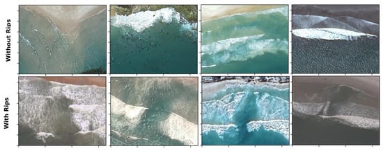
Figure 1.
Example aerial images from Google Earth which are used to train the present AI-based model. The top row contains example images without rip currents, while the bottom row contains example images with rip currents.
The training dataset and labels are used to modify the weights of the AI-based model. In the present case, 80% of the training dataset (consisting of 1740 images of rip currents and 700 no rip currents, in total 2440 images) was used. The remaining 20% (488 images) was used for validation, which was used for monitoring the model’s performance while training. The validation dataset enables the tuning of the hyperparameters, such as how fast the model learns (learning rate) or whether the model is overfitting or poorly generalizing [38].
The testing dataset is used to independently assess the performance of the AI-based model and has been made open access by [6]. The testing dataset consists of 23 video clips with a total of 18,042 frames (9053 frames with rips and 8989 without rips), and these results are discussed in Section 3. This dataset contains oblique videos which could mimic the setting of a beach-mounted camera used in the context of monitoring or surf-life saving.
2.2. Model Architecture and Training
Two model architectures were used in the process of model training, a baseline 3-layer CNN and a pre-trained CNN MobileNet model (original version), referred to as MobileNet from hereon. The general architecture and description of a CNN model is illustrated in Figure 2 [39]. Further detail regarding the model architectures used are provided in Table 1. The Mobile-Net model differs slightly from Figure 2 and consists of residual blocks which have dramatically reduced the vanishing gradient problem that commonly occurred in deeper model architectures [40], while promoting stability in the process of model training [41]. MobileNet also uses depth-wise convolutional, which has also dramatically reduced the number of weights in CNNs, thus making them suitable for mobile devices. While there exists a wide variety of notable alternatives to MobileNet that typically have more model parameters (e.g., Res-Net50 or VGG-16), they did not show any significant improvements in accuracy when applied to our problem of rip current classification. Moreover, we selected the model that had the fewest number of parameters that achieved the highest accuracy, which in this case was MobileNet. Overall, we found that MobileNet performed best in terms of “model interpretability”. In the present study, a more traditional deep-learning classification models, as outlined in Table 1, was used, as opposed to regionally confined-based CNNs (R-CNNs) or YOLO-based architectures [42,43]. While RCNNs and YOLO type model architectures for object localization have certainly been successful in the domain of computer vision, they are not interpretable.
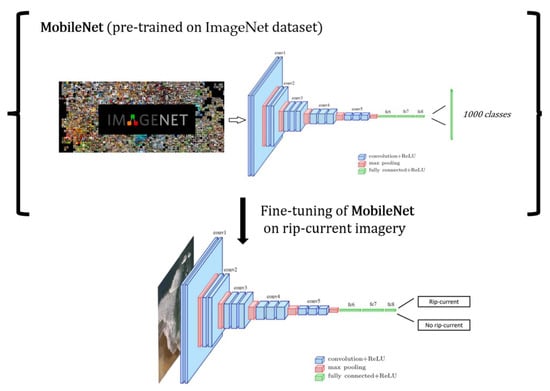
Figure 2.
The general application of applying transfer learning. First, a CNN (MobileNet) is trained on an extremely large dataset. Next, the CNN is fine-tuned on a smaller dataset. The architecture of a CNN consists of convolutional layers (blue), which have a series of convolutional kernels that extract features from the images. The maximum pooling (red) layers help reduce the dimensionality of the data and discard redundant features. Finally, the fully connected layers (green) further reduce the dimensionality of the data into a compressed latent representation. The final layer makes a prediction into two classes: rip current or no rip current.

Table 1.
Architectures of the convolutional neural networks (CNN) used within this study.
The present study consists of two model training strategies: (1) only training on the rip current dataset, (2) transfer-learning on ImageNet [44]. Transfer-learning (model pre-training) is typically used in problems where the data size is limited, and the number of model parameters is large. Transfer-learning can significantly improve model generalization or testing accuracy, where large models like MobileNet can easily suffer from overfitting. Transfer-learning is performed as follows: a model is first trained on an extremely large dataset (e.g., ImageNet consisting of 1000 categories [45]). Then, the model is fine-tuned on a smaller dataset (e.g., rip current classification), where the learned features/model weights from the large dataset can help the model converge more rapidly on the small dataset, as illustrated in Figure 2. The pre-trained MobileNet model on the ImageNet dataset is open-access and is freely available to use through commonly used deep learning libraries such as tensorflow and pytorch. The following process is applied to fine-tune the MobileNet model on our rip current dataset:
- The MobileNet classification head, which predicts 1000 different categories, is replaced with a new classification head consisting of only two categories—rip current and no rip current.
- Weights in the MobileNet model are frozen, and thus many layers and their corresponding weights are not trainable. Weights in deeper layers of the network are only made trainable.
The above methodology is widely used in many applications of transfer learning [46]. However, there are many variations to the above methodology, which include removing and replacing deeper or more abstract layers in the network and changing the number of layers that are frozen during training. The concept of freezing model layers is very beneficial to datasets of small size (e.g., 1000 s of images), as it can help model convergence and improve model generalization. Through experimentation, the best accuracy was found through generalization when all model weights were trainable (no freezing of model weights), where overfitting was controlled through dropout, learning rate decay and early stopping. Further detail about model training is outlined in the results section.
To further quantify uncertainty or variability in model accuracy, a K-fold validation was performed. K-fold validation is performed in the following manner, in which the training dataset is split into 5 partitions, where 4 partitions are reserved for training and 1 partition is reserved for validation/tuning of the model hyperparameters. This process is repeated 5 times. While the validation dataset is different through each iteration of K-fold, model evaluation is only performed on the independent test set, which is fixed.
AI-based algorithms learn from training data through minimizing a cost function. In the present study, a binary cross entropy cost function was used, which is a measure of difference between two probability distributions. Here, the binary cross entropy measures the differences in distributions between the model predictions (probabilistic predictions) and the observed events (e.g., rip current or not). The learning rate influences how much acquired information from the training data overrides old information, and the models are trained with an initial learning rate of 10−3, and through the Adam optimizer [47]. To ensure that the models do not overfit, the learning rate is adapted through regular monitoring of the validation cost function (on the validation dataset). The learning rate is reduced by a factor of 3 if the validation loss does not decrease after three epochs. Furthermore, if the validation loss fails to reduce after 10 epochs, training is stopped. To monitor the performance of the model, the accuracy score metric is used, which is defined as the percentage of correct predictions made by the model on the testing dataset. The models were trained on a NVIDIA P100 Graphics Processing Unit (GPU) with 12 GB of RAM, with a batch-size of 32. Model training times vary as a function of model architecture and are longest for training the MobileNet, where all weights are trainable. Data augmentation was performed during training through the Tensorflow Data Application Programing Interface. Training times are approximately 30 s per epoch, where the model typically converges after 40–50 epochs, thus taking approximately 20–25 min to train the model. The 3-layer CNN can take 5–10 min to train.
2.3. Interpretable AI
Interpretable AI is used for two key purposes in this study: (1) to localize the rip current within image and (2) to improve model development. Interpretable AI addresses the narrative that deep learning models are simply just ‘black boxes’ due to their perceived inability to understand how a particular prediction was made (e.g., [48]). A model that is both precise and interpretable is important for building trust in the prediction and further development in the understanding of complex systems such as rip currents [36,49,50]). In this study, a gradient-weighted class-activation map (Grad-CAM, [36]) was implemented to better understand how the CNN made a certain prediction of a rip current for a given beach. In the context of rip current detection, Grad-CAM identified spatial locations within an image or video, for a given model, that most strongly supported the prediction (e.g., rip current or no rip current) from the model.
For object localization/detection, the present approach is semi-supervised, (1) first a classification model is trained and predicts whether a rip current exists within an image, (2) then the interpretable AI algorithm, namely Grad-CAM, is used to localize where the rip current is located within an image. The python package tf-explain was used for Grad-CAM implementation [51]. For each image, Grad-CAM predicts a pixel-wise activation/intensity of pixel importance. These pixel-wise activations are normalized to the range [0, 1] domain. Pixels with activations >0.5 are considered important, and lower importance pixels (<0.5) are masked. Given that rips currents do not have a well-defined shape (amorphous), the semi-supervised approach is more appropriate as it enables the model to learn spatial characteristics without the additional constraints that R-CNNs have.
In a well-trained model, locations around or nearby the rip current are expected to influence the model’s prediction most strongly. However, a poorly trained model may look at irrelevant features (e.g., the coastline or labels and text contained in the image) to make predictions, as illustrated in Figure 3b, where the model focuses on the NOAA label in the top left corner and regions surrounding the rip current rather than the rip current itself. Clearly, in this instance, the model struggles to generalize from the aerial imagery that it is trained on to this example from an oblique angle, as illustrated in Figure 3b. Many of these issues are subsequently improved by augmenting the training dataset. Examples of augmentation include perspective augmentation, where the image is sheared or rotated to appear like an oblique image. Figure 3d shows that when a model is well-trained it focuses on features associated with the rip current, and thus can generalize well to images it has never seen before. Interestingly, in this instance (Figure 3a), the poorly trained model predicts the correct classification for that given image. However, as illustrated by Grad-CAM in Figure 3b, it is not using the right information or spatial features to make that decision. Moreover, this is an example where the correct prediction is made for the wrong reasons. A human or a well-trained model knows that information contained inthe NOAA label is useless to the prediction of rip current, but in the poorly trained model, the label is clearly influencing the model’s prediction.
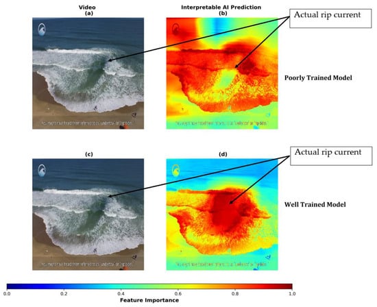
Figure 3.
An illustration of the pixel importance plot for the identification of a rip current in a poorly trained model, where the model is predicting that a rip current is occurring, but for the wrong reasons. Here, warm colors indicate more importance and cool colors indicate less importance. The model focuses on the beach/people rather than the rip current itself, indicated by the red colors over the coastline.
There are many instances where systematic errors in model generalization can be identified through Grad-CAM. While Grad-CAM provides an alternative measure to model performance/generalization, it also provides an opportunity to localize where rips currents are occurring within each image, which is useful for monitoring rip currents on popular beaches. In the context of data labelling, manually labelling bounding boxes around rips is a very time-consuming process and does not fully characterize the complex morphology of rips. From a model development perspective, this is particularly useful as it can help identify systematic deficiencies within the model, which could not otherwise be found using traditional machine learning methods [48].
2.3.1. Model Development
Traditional metrics such as accuracy score (f1_score, true positives etc.) are useless when the AI-based model predicts the correct category, but for the wrong reasons, as illustrated in Figure 3. Therefore, it is often challenging to understand subjectively how a model is performing, which is crucial in applications where human safety is of concern, such as rip current detection. However, in the present study, a new method for model development is introduced, where we use interpretable AI to learn systematic deficiencies within our AI-based models and adopt data augmentation schemes to mitigate their effects (e.g., poor model generalization in certain environmental conditions).
Without Interpretable AI, only objective measures of performance are possible, through success metrics (e.g., accuracy score, confusion matrix, f1_score). Model development and improvement is thus challenging and tedious as these metrics are very objective, and do not directly suggest areas of potential improvement. However, with interpretable AI, a further screening is possible and thus adds another layer of verification of the algorithm through Grad-CAM and examines what spatial characteristics influenced the model’s prediction. Moreover, this interpretable AI scheme, for model development, enables a deeper understanding of how the quality and diversity of data affects model skill.
The model development cycle with interpretable AI (as illustrated in Figure 4) can be described as follows:
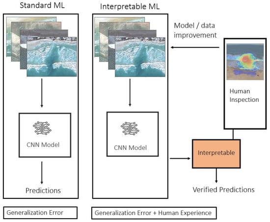
Figure 4.
An illustration of our model training/improvement scheme. The standard AI approach is outlined on the left, with our Interpretable AI strategy outlined on the right. The interpretable AI strategy for model training/improvement uses Grad-CAM as interpretable AI step to create verified predictions (via human inspection) that can improve model development.
- (1)
- Train AI-based model initially on training dataset (images of rip currents),
- (2)
- Evaluate traditional performance metrics (e.g., accuracy score) and Grad-CAM heatmaps for each prediction,
- (3)
- Predictions from the AI-based model (Grad-CAM) are thoroughly screened to identify whether there are systematic issues in the model (e.g., is Grad-CAM performing more poorly in some videos than others),
- (4)
- Devise a data augmentation scheme to mitigate these systematic issues.
To overcome the lack of diversity in the model training data, a data augmentation strategy is used to enhance the size of the model training data, where data augmentation is defined as synthetic enhancement of the original size of the training dataset. Data augmentation is performed through applying a series of random transformations to the images while the model was training. While synthetic data is not a perfect solution to increasing data size, it is both faster and easier to implement than increasing the size of the training data through manually labelling images from archives of beach mounted cameras. The process of applying steps 1–4 is rather repetitive and requires some trial and error. In the first iteration of testing, the models were first trained without any augmentation. Then, the model was evaluated to check its ability to localize rip currents through using the feature importance heatmap from Grad-CAM. Both trivial and difficult cases were identified, the latter being where the model had issues (scenarios where the positioning of the rip current was incorrect). A set of trivial and difficult were used to classify examples, which were used to evaluate the model performance in subsequent iterations. In addition to identifying systematic issues in the model through Grad-CAM (step 3), in subsequent iterations of training, an assessment was performed to understand how changing or adding an additional data augmentation scheme would change the Grad-CAM heatmaps in the trivial and difficult-to-classify examples.
For example, when initially training the AI-based model, it struggled with oblique images. Thus, perspective transforms and translations were introduced as augmentations schemes. Some examples of data augmentation are provided in Figure 5 through the ‘albumentations’ python library [52]. Additionally, it was found that introducing random shadows, and random rain and fog, were useful for mitigating issues illustrated in Figure 3. Systematic inaccuracies were also found in images where the beach occupied a large portion of the image. These problems were mitigated through the comprehensive augmentation scheme, as described in Table 2. For example, to generalize to domains consisting of rocky outcrops we found techniques such as channel shuffling and channel shifting (constant value is added to each channel) as the most effective augmentation technique. While the training dataset does consist of rip currents within proximity to rocky outcrops, we found it would fail in almost all instances where rocky outcrops or dark objects occurred within the test dataset. We find that the channel shuffling and shifting reduces the importance of background color to the CNN, thus helping it generalize better. Additionally, the introduction of the perspective transformations dramatically improved the model accuracy and its ability to localize rip currents that were from oblique angles. Perspective transformations aim to distort the view of the original images so that we can synthetically generate these images from an alternative perspective. Overall, we found this augmentation to be the most important for model generalization.
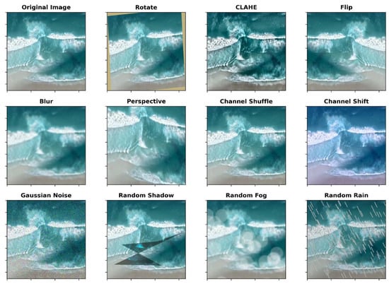
Figure 5.
Examples of different image augmentation techniques used in the process of training. Other augmentations were also used in addition to the eight illustrated. CLAHE stands for contrast limited adaptive histogram equalization.
Table 2.
Examples of the criteria required to assemble a training dataset for rip current classification. Augmentation strategies to synthetically generate training samples are also outlined.
In previous work by [6], the data augmentation was limited to rotating the images 90° either side. Our approach to data augmentation could also be beneficial for object detection methods such as Faster R-CNN or YOLO, as augmentations such as image-shearing, perspective transformations, and image zooming can also be applied to the bounding box coordinates. The present study extends this to include augmentations such as perspective transformations, and the augmentation of random rain, fog, and shadows. In our application of the augmentation scheme for each iteration (per batch), each type of augmentation (e.g., rotation) has a 50% chance of occurring. Thus, at each individual iteration during training, multiple types of augmentations were applied to a batch of images (e.g., random rain and rotation). For augmentations such as rotation or shearing, we used reflection padding, in which pixels beyond the edge are reflected to fill in the missing values. We also explored using edge padding, but it made little difference to our results. We also highlight that we include additional transformations such as random rain, fog, and shadows which, in this piece of work, did not result in any improvement in our results. However, it is important that we highlight and bring awareness to other alternative techniques to synthetically enhance our data, as such methods could help our model generalize to more complex and diverse environments.
3. Results
The two models outlined in Table 2 were applied to a series of 23 testing videos, with and without rips currents, and compared to the Faster R-CNN model trained by [6]. In Figure 6, the percentage accuracy score of each training method is presented for all 23 testing videos. The present results demonstrate that transfer-learning and data augmentation improve the overall accuracy score of the model on the test dataset. It is important that we highlight that the validation accuracy (on aerial imagery) varies significantly from the overall test accuracy (oblique imagery). All model configurations achieved at least 90% K-fold accuracy on the validation dataset, however very different results were obtained for the independent test dataset.
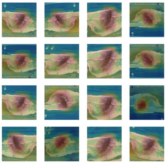
Figure 6.
An illustration of how the Grad-CAM heatmap can generalize to input images from a wide variety of different perspectives.
Without augmentation and transfer learning, the CNN model struggles to generalize well on the test set and achieves a maximum accuracy of about 0.59 (or 59%) and an average K-fold accuracy of 0.51, as illustrated in Table 3—which is not useful in a real-world context. When data augmentation is used, the accuracy dramatically increases to 0.75, with a K-fold accuracy of 0.69. Similarly, MobileNet, without transfer learning or augmentation (weights are not initialized from ImageNet), has little or no accuracy at 0.51, and a K-fold accuracy of 0.48. When augmentation or transfer learning on ImageNet [44] is used alone the accuracy improves to 0.68 and 0.70, respectively. However, when augmentation and transfer learning are used collectively, we obtained a maximum accuracy of 0.89 and a K-fold accuracy of 0.85. The confusion matrix for the MobileNet model which uses augmentation and transfer learning is illustrated in Table 4. Overall, the accuracy for each class (rip current or no rip current) is relatively equally balanced.
Table 3.
The accuracy score across all videos across all model training configurations used in this study, the K-fold model accuracy is provided in brackets which is averaged across all folds. The non-bracketed value is the maximum accuracy achieved.
Table 4.
Confusion matrix on the testing dataset for the best performing MobileNet model with transfer learning and augmentation.
Overall, these experiments highlight the value of both transfer learning and data augmentation in an image classification context. Augmentation alone adds significant value to the 3-layer CNN, resulting in a 75% accuracy, but with the MobileNet model we are unable to achieve a significant accuracy through augmentation alone. This is likely due to the MobileNet model being overparameterized and the number of parameters in the model making it extremely challenging to train, and thus for the model’s loss function to converge. Similarly, with transfer-learning alone, the MobileNet model still struggles to generalize well to the testing dataset. Here, the model is no longer overparameterized, as only several layers are tunable. Moreover, our results suggest that the lack of diversity in the training data is a limiting factor in the model’s accuracy and its ability to generalize. However, when augmentation and transfer learning are combined, the accuracy dramatically improves.
Upon applying the interpretable AI method (Grad-CAM) to each of the models, it became clear that poorer performing models tend to focus on other objects such as trees, coastlines, rocks, and people instead of the rip currents (e.g., Figure 3). Even in scenarios where the model prediction is correct, the heatmap from Grad-CAM illustrates that the model is not ‘looking’ at the correct features—a clear indication of poor model generalization. We further tested whether our best performing model would generalize to the testing dataset when augmentation was applied (e.g., random rain and perspective transformations), and the accuracy scores remained relatively unchanged. This is further illustrated in Figure 6, where a Grad-CAM heatmap consistently rotates with the rotation of the input image.
Note that in the present approach no aggregates or average predictions are required from the AI-based model. Accuracy metrics for the model are provided for each video in the testing dataset and are benchmarked against [6] in Table A1 of the Appendix A.
Overall, through using Grad-CAM, interpretable AI-method, the present study’s model is able to accurately localize the position of a rip current. The position of a rip current can be localized by examining the heatmap of pixel importance for a prediction made by the MobileNet model (or any CNN in general). In Figure 7, the leftmost column, the most important pixels are the warmest (reddest) and align strongly to the position of the actual rip current. Grad-CAM is also able to capture some characteristics of the amorphous structure of the rip current. This approach to localization of a rip current differs significantly from existing AI methods, which identify the bounding box in which the rip current is located within. The examples shown in Figure 7 are from the test dataset provided by [6]. It is important to emphasized that this approach was applied to all 23 videos, and performs well across nearly all videos, aside from the videos named: rip_03.mp4, rip_05.mp4, and rip_15.mp4, where the performance/accuracy is lower. Examples of poorly classified images are given in Figure A1 in the Appendix A.
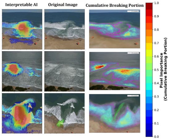
Figure 7.
A comparison of rip detection using interpretable AI (left panels) compared to the cumulative breaking portion (right panels) with a still frame of the videos shown in the center panels. Note that for the Interpretable AI (left panel), the warmer the color, the more important that pixel is for the prediction of a rip current. For the cumulative breaking portion (right panel), the warmer the color, the more breaking wave intensity within a pixel. The 10th percent exceedance contour is outlined in magenta. The shape of the 10th percent exceedance contour provides a relatively robust marking of the edge of wave breaking, defining the rip current boundary.
To ensure the boundaries of the rip currents as predicted by the interpretable AI are realistic, a comparison was made between the predicted boundaries and those identified using more traditional image processing techniques. Traditional image processing techniques (after [16,53]) tend to utilize the average pixel intensity over a fixed duration to determine areas of wave breaking (lighter areas corresponding to broken whitewater) and non-breaking (darker areas without whitewater present). However, such approaches may lose considerable information during the averaging process and require further thresholding and interpretation to quantify areas of non-breaking. An alternative approach, [54] identified the area of wave breaking for each frame and summed these areas as a cumulative breaking portion during the observation period. The threshold for defining breaking within individual frames is a variable, yet provides more control and definition than time-averaged techniques. A breaking exceedance value can then be extracted from the cumulative breaking portion, as illustrated in Figure 7 (right panels), where a 10% exceedance value has been plotted over the equivalent time-averaged image. A rip current is assumed where breaking is not occurring or occurring a low proportion of the time. Overall, the AI-predicted boundaries are consistent with those identified by the cumulative breaking portion. It should also be noted that the image processing technique is limited in requiring a sequence of images or video taken from a relatively stable platform and is not necessarily identifying a rip, but rather areas where breaking is not occurring, which usually correspond to a rip current. Rip currents of short temporal duration (flash rips) or rip currents containing large amounts of foam are unlikely to be well-resolved using this method.
4. Discussion
The present study’s overall accuracy does not exceed the 0.98 accuracy obtained by [6] in their framed aggregation approach (F-RCNN + FA), but matches closely with their results without frame aggregation (FA). Through further fine-tuning of the present model, a higher accuracy could be achieved. There are several advantages to using Grad-CAM for localization of rip currents over traditional approaches (Faster R-CNN in [6]). Firstly, this approach is semi-supervised (in the context of object localization) and there is no penalization (during model training) on the CNNs prediction of the position of the rip current within an image, unlike in Faster R-CNN or YOLO. This means that there is no need to provide the bounding box for where the rip current is located, which is a time-consuming process for labelling image data. While Faster R-CNN algorithms are very useful in many different applications, by penalizing the algorithm on where the rip current is positioned, it tends to constrain the algorithm/model to only learn features that are specific to localizing rip currents within the labelled bounding box. Moreover, this means that algorithms such as Faster R-CNN and YOLO could perhaps be less flexible on the features/information that they can learn. Moreover, we have demonstrated that it is possible to “localize” rip currents relatively precisely without informing the model where the rip current is within the image. Object detectors such as Faster R-CNN (as implemented in [6]) cannot operate in real-time and are often not mobile friendly. Our approach of image classification can run in excess of several hundred frames per second on GPU (~400) and in real-time on a CPU (20–30 fps). However, our interpretable AI method of Grad-CAM can only run at approximately 6–10 frames per second on a CPU and GPU. However, given that rip currents are not present all the time, our interpretable AI method can be run on-demand. Applying our method of Grad-CAM has currently not been optimized, and further improvement in speed is likely possible. The lightweight nature of MobileNet means it can be deployed on lightweight devices such as mobile phones or drones, unlike Faster R-CNN. It is important that we highlight that there are alternatives to Faster R-CNN, such as the YOLO object detection algorithm, in which some variants can run on mobile devices and in real-time.
Secondly, interpretable AI model development can also be subjective and be further improved through human experience. This subjective element is important, as understanding “the why” of how an AI algorithm makes a particular prediction reduces the black box and adds this additional level of confidence that the user has with the AI. Furthermore, subjective quality control is also very important for applications such as deploying this method to aid surf lifeguards. In the context of real-time model deployment (e.g., applied to beach mounted cameras or drones), interpretable AI has the potential to identify model drift, defined as changes in the model accuracy, or scenarios where the equipment is performing poorly.
Thirdly, the interpretable framework enables the training of effective models, and thus informs future developments, and potential limitations within the data, as illustrated in the life cycle of interpretable AI development in Figure 4. The outline of how Grad-CAM could help easily identify issues within the AI-based models, and devising data augmentation strategies to overcome them, is elaborated in Section 2.
Method Comparison
Both techniques in artificial intelligence (interpretable AI and CNNs) can be used to classify and localize rip currents. However, it is important that the limitations in these methods are pointed out and compared to existing technologies that could also be deployed. While human observation will continue to be an important approach to rip current detection [12], other approaches using imagery or video feeds will require deployment of cameras onto a wide variety of beaches. Furthermore, the cameras need to have unobstructed views of the beach and need ongoing maintenance. While the task of large-scale deployment of cameras through beaches is an expensive task, it would fundamentally change beach safety, and would have a huge impact on beaches where lifeguards are off duty or not present at all. This AI technology also opens the door for remotely sense patrol patterns making use of drone technology. Early notifications through applications could take rip current-related rescue from reactive to preventative, especially given the low numbers of beachgoers who are able to identify rip currents [12]. This is especially true, as rip currents are the leading cause of drownings (on wave exposed beaches) worldwide [12].
In Table 5. the advantage and disadvantages of several rip current detection methods are given. These include well-established image processing techniques. In Table 5, some limitations with AI methods are also given, which include poor model generalization and resolving the complex, amorphous structure of rip currents. This study has highlighted that with careful consideration of data augmentation (outlined in Section 2.3.1) and interpretable AI, improvement over the existing limitations of AI can be made.
Table 5.
Advantages and disadvantages of the methods discussed in the present study.
5. Conclusions
The present study investigates the remote identification of rip currents using visual data from cameras and videos. More specifically, the use of artificial intelligence was investigated based on a review of the current status quo. Several recent studies have reported great progress in the field of object or feature detection, with particular focus on rip currents. Although these studies have reported great success in their identification accuracy, they were limited by requiring a bounding box in the images. These boxes also limited the AI method’s ability to learn features other than rip currents and thus limited generalization of those methods. The interpretable AI model presented here circumnavigated that limitation and thus enables the deployment of the new rip current identification tool in more application. The method presented here also made use of a synthetic data augmentation strategy that enables the model to generalize even further and thus became more independent on practical constraints. These include rain on the camera lens, fog, varying sand exposer (tides), and image and video capturing perspective angles. A detailed list of model performance metric is provided with the newly proposed method, obtaining an overall accuracy of 89% (based on the test data sets—23 videos). Although this number is lower than other methods, the flexibility of this method makes it attractive and still presents the opportunity for further optimization. Established image processing techniques are also discussed, as these are widely used and reliable. To highlight the functionality of these methods, an advantages and disadvantages table has been added as a part of the discussion. This will enable the reader to get a clear and quick understanding of which methods will be the best solution to a problem. The future prospect of this study is to test and validate this method in using drone technology as well. This will enable monitoring of beaches and move rip current-related incidents from a reactive to a preventative approach. This will also enable the monitoring of large beaches, which will then not be constrained to the perspective of singular cameras.
There are certainly many challenges regarding detecting different types of rip currents, including feeder rip currents and images containing multiple rip currents. The current approach demonstrates significant skill in the localization of single rip currents through interpretable AI. Future work will focus on examining whether Grad-CAM can detect multiple rip currents in one image, such as feeder rip currents, which may require further refinement or enhancement of training data and revisions to the Grad-CAM technique. Further work will also investigate the amorphous structure of rip currents, including the ability to capture shape characteristics such as width and length. We will also measure other accuracy metrics in the context of object localization, such as Intersection of Union (IOU) score. A more diverse range of coastlines should also be considered, and in different environmental conditions, as this will further help progress the understanding of how data augmentation can help the models generalize. As AI becomes data-centric, the focus will be on improving the data rather than the models themselves. Both data augmentation and interpretable AI can help in understanding how to better improve the training data so that a better model generalization may be obtained. Further studies will also investigate how these techniques can be deployed in an operational setting, e.g., making use of drones. These can then be used to patrol remote or large beaches, beyond the sight of lifeguards and fixed camera angles. Here, the model generalization will be even more important.
Author Contributions
C.R. conceived the research and study structure. N.R., C.R. and T.S. wrote the manuscript. N.R. conducted all the AI-related model development and processing. T.S. contributed insight into the other image processing techniques. C.R. and T.S. reviewed the manuscript. All authors provided critical feedback and contributed to revisions and rewrites of the manuscript. A.W. provided practical context and need for the research. All authors have read and agreed to the published version of the manuscript.
Funding
This research was funded by the National Institute of Water and Atmospheric Research (NIWA) Taihoro Nukurangi, Strategic Scientific Investment Fund work program on “Hazards Exposure and Vulnerability” [CARH22/3 02]. The authors wish to acknowledge the use of New Zealand eScience Infrastructure (NeSI) high performance computing facilities as part of this research. New Zealand’s national facilities are provided by NeSI and funded jointly by NeSI’s collaborator institutions and through the Ministry of Business, Innovation & Employment’s Research Infrastructure program. https://www.nesi.org.nz.
Data Availability Statement
The data used for training the AI-based model is freely available at https://sites.google.com/view/ripcurrentdetection/download-data (accessed on 25 August 2022), as provided by [6]. The MobileNet model used in the present study is publicly accessible through the tensorflow Python application programming interface (https://www.tensorflow.org/api_docs/python/tf/keras/applications/mobilenet/MobileNet (accessed on 25 August 2022)). Data augmentation was performed using the albumentations package (https://albumentations.ai/ (accessed on 25 August 2022)) which is configured through the Tensorflow Data Interface (https://www.tensorflow.org/guide/data (accessed on 25 August 2022)), which are both publicly available and free. Lastly the interpretable AI algorithm used in the present study is also freely available and accessible through Python (https://github.com/sicara/tf-explain (accessed on 25 August 2022)).
Acknowledgments
We would like to acknowledge Surf Life Saving New Zealand for identifying the need for this research and tool development. Surf Life Saving New Zealand also provided support in collecting images of rip-currents for this study. We also acknowledge the standing Memorandum of Understanding (MoU) between the National Institute of Water and Atmospheric Research (NIWA) and SLSNZ and look forward to deploying this new technology in an operational setting.
Conflicts of Interest
The authors declare no conflict of interest.
Appendix A
Table A1.
The accuracy scores of several benchmark models against [6], the accuracy scores were also reported for human annotators. Human annotators were asked to localize and determine whether a rip current occurs within each frame and were not carefully trained (unlike surf-life savers). Note, each video is weighted equally when computing the overall accuracy score.

Figure A1.
Examples of poorly identified rip currents using Interpretable AI.

References
- Castelle, B.; Scott, T.; Brander, R.W.; McCarroll, R.J. Rip current types, circulation and hazard. Earth Sci. Rev. 2016, 163, 1–21. [Google Scholar] [CrossRef]
- Dusek, G.; Seim, H. A Probabilistic Rip Current Forecast Model. J. Coast. Res. 2013, 29, 909–925. [Google Scholar] [CrossRef]
- Arun Kumar, S.V.V.; Prasad, K.V.S.R. Rip current-related fatalities in India: A new predictive risk scale for forecasting rip currents. Nat. Hazards 2014, 70, 313–335. [Google Scholar] [CrossRef]
- Mucerino, L.; Carpi, L.; Schiaffino, C.F.; Pranzini, E.; Sessa, E.; Ferrari, M. Rip current hazard assessment on a sandy beach in Liguria, NW Mediterranean. Nat. Hazards 2021, 105, 137–156. [Google Scholar] [CrossRef]
- Zhang, Y.; Huang, W.; Liu, X.; Zhang, C.; Xu, G.; Wang, B. Rip current hazard at coastal recreational beaches in China. Ocean. Coast. Manag. 2021, 210, 105734. [Google Scholar] [CrossRef]
- de Silva, A.; Mori, I.; Dusek, G.; Davis, J.; Pang, A. Automated rip current detection with region based convolutional neural networks. Coast. Eng. 2021, 166, 103859. [Google Scholar] [CrossRef]
- Voulgaris, G.; Kumar, N.; Warner, J.C. Methodology for Prediction of Rip Currents Using a Three-Dimensional Numerical, Coupled, Wave Current Model; CRC Press: Boca Raton, FL, USA, 2011. [Google Scholar]
- Brander, R.; Dominey-Howes, D.; Champion, C.; del Vecchio, O.; Brighton, B. Brief Communication: A new perspective on the Australian rip current hazard. Nat. Hazards Earth Syst. Sci. 2013, 13, 1687–1690. [Google Scholar] [CrossRef]
- Moulton, M.; Dusek, G.; Elgar, S.; Raubenheimer, B. Comparison of Rip Current Hazard Likelihood Forecasts with Observed Rip Current Speeds. Weather Forecast. 2017, 32, 1659–1666. [Google Scholar] [CrossRef]
- Carey, W.; Rogers, S. Rip Currents—Coordinating Coastal Research, Outreach and Forecast Methodologies to Improve Public Safety. In Proceedings of the Solutions to Coastal Disasters Conference 2005, Charleston, SC, USA, 8–11 May 2005; pp. 285–296. [Google Scholar]
- Brander, R.; Bradstreet, A.; Sherker, S.; MacMahan, J. Responses of Swimmers Caught in Rip Currents: Perspectives on Mitigating the Global Rip Current Hazard. Int. J. Aquat. Res. Educ. 2016, 5, 11. [Google Scholar] [CrossRef][Green Version]
- Pitman, S.J.; Thompson, K.; Hart, D.E.; Moran, K.; Gallop, S.L.; Brander, R.W.; Wooler, A. Beachgoers’ ability to identify rip currents at a beach in situ. Nat. Hazards Earth Syst. Sci. 2021, 21, 115–128. [Google Scholar] [CrossRef]
- Brander, R.; Scott, T. Science of the rip current hazard. In The Science of Beach Lifeguarding; Tipton, M., Wooler, A., Eds.; Taylor & Francis Group: Boca Raton, FL, USA, 2016; pp. 67–85. [Google Scholar]
- Austin, M.J.; Scott, T.M.; Russell, P.E.; Masselink, G. Rip Current Prediction: Development, Validation, and Evaluation of an Operational Tool. J. Coast. Res. 2012, 29, 283–300. [Google Scholar]
- Smit, M.W.J.; Aarninkhof, S.G.J.; Wijnberg, K.M.; González, M.; Kingston, K.S.; Southgate, H.N.; Ruessink, B.G.; Holman, R.A.; Siegle, E.; Davidson, M.; et al. The role of video imagery in predicting daily to monthly coastal evolution. Coast. Eng. 2007, 54, 539–553. [Google Scholar] [CrossRef]
- Lippmann, T.C.; Holman, R.A. Quantification of sand bar morphology: A video technique based on wave dissipation. J. Geophys. Res. Ocean. 1989, 94, 995–1011. [Google Scholar] [CrossRef]
- Holman, R.A.; Lippmann, T.C.; O’Neill, P.V.; Hathaway, K. Video estimation of subaerial beach profiles. Mar. Geol. 1991, 97, 225–231. [Google Scholar] [CrossRef]
- Holman, R.A.; Stanley, J. The history and technical capabilities of Argus. Coast. Eng. 2007, 54, 477–491. [Google Scholar] [CrossRef]
- Bogle, J.A.; Bryan, K.R.; Black, K.P.; Hume, T.M.; Healy, T.R. Video Observations of Rip Formation and Evolution. J. Coast. Res. 2001, 117–127. [Google Scholar]
- Taborda, R.; Silva, A. COSMOS: A lightweight coastal video monitoring system. Comput. Geosci. 2012, 49, 248–255. [Google Scholar] [CrossRef]
- Nieto, M.A.; Garau, B.; Balle, S.; Simarro, G.; Zarruk, G.A.; Ortiz, A.; Tintoré, J.; Álvarez-Ellacuría, A.; Gómez-Pujol, L.; Orfila, A. An open source, low cost video-based coastal monitoring system. Earth Surf. Process. Landf. 2010, 35, 1712–1719. [Google Scholar] [CrossRef]
- Brignone, M.; Schiaffino, C.F.; Isla, F.I.; Ferrari, M. A system for beach video-monitoring: Beachkeeper plus. Comput. Geosci. 2012, 49, 53–61. [Google Scholar] [CrossRef]
- Simarro, G.; Ribas, F.; Álvarez, A.; Guillén, J.; Chic, Ò.; Orfila, A. ULISES: An Open Source Code for Extrinsic Calibrations and Planview Generations in Coastal Video Monitoring Systems. J. Coast. Res. 2017, 33, 1217–1227. [Google Scholar] [CrossRef]
- Liu, Y.; Wu, C.H. Lifeguarding Operational Camera Kiosk System (LOCKS) for flash rip warning: Development and application. Coast. Eng. 2019, 152, 103537. [Google Scholar] [CrossRef]
- Mori, I.; de Silva, A.; Dusek, G.; Davis, J.; Pang, A. Flow-Based Rip Current Detection and Visualization. IEEE Access 2022, 10, 6483–6495. [Google Scholar] [CrossRef]
- Rashid, A.H.; Razzak, I.; Tanveer, M.; Hobbs, M. Reducing rip current drowning: An improved residual based lightweight deep architecture for rip detection. ISA Trans. 2022, in press. [Google Scholar] [CrossRef]
- Maryan, C.C. Detecting Rip Currents from Images. Ph.D. Thesis, University of New Orleans, New Orleans, LA, USA, 2018. [Google Scholar]
- Stringari, C.E.; Harris, D.L.; Power, H.E. A novel machine learning algorithm for tracking remotely sensed waves in the surf zone. Coast. Eng. 2019, 147, 149–158. [Google Scholar] [CrossRef]
- Sáez, F.J.; Catalán, P.A.; Valle, C. Wave-by-wave nearshore wave breaking identification using U-Net. Coast. Eng. 2021, 170, 104021. [Google Scholar] [CrossRef]
- Liu, B.; Yang, B.; Masoud-Ansari, S.; Wang, H.; Gahegan, M. Coastal Image Classification and Pattern Recognition: Tairua Beach, New Zealand. Sensors 2021, 21, 7352. [Google Scholar] [CrossRef] [PubMed]
- Dérian, P.; Almar, R. Wavelet-Based Optical Flow Estimation of Instant Surface Currents From Shore-Based and UAV Videos. IEEE Trans. Geosci. Remote Sens. 2017, 55, 5790–5797. [Google Scholar] [CrossRef]
- Radermacher, M.; de Schipper, M.A.; Reniers, A.J.H.M. Sensitivity of rip current forecasts to errors in remotely-sensed bathymetry. Coast. Eng. 2018, 135, 66–76. [Google Scholar] [CrossRef]
- Anderson, D.; Bak, A.S.; Brodie, K.L.; Cohn, N.; Holman, R.A.; Stanley, J. Quantifying Optically Derived Two-Dimensional Wave-Averaged Currents in the Surf Zone. Remote Sens. 2021, 13, 690. [Google Scholar] [CrossRef]
- Rodríguez-Padilla, I.; Castelle, B.; Marieu, V.; Bonneton, P.; Mouragues, A.; Martins, K.; Morichon, D. Wave-Filtered Surf Zone Circulation under High-Energy Waves Derived from Video-Based Optical Systems. Remote Sens. 2021, 13, 1874. [Google Scholar] [CrossRef]
- Ellenson, A.N.; Simmons, J.A.; Wilson, G.W.; Hesser, T.J.; Splinter, K.D. Beach state recognition using argus imagery and convolutional neural networks. Remote Sens. 2020, 12, 3953. [Google Scholar] [CrossRef]
- Selvaraju, R.R.; Cogswell, M.; Das, A.; Vedantam, R.; Parikh, D.; Batra, D. Grad-cam: Visual explanations from deep networks via gradient-based localization. In Proceedings of the IEEE International Conference on Computer Vision, Venice, Italy, 22–29 October 2017. [Google Scholar]
- Linardatos, P.; Papastefanopoulos, V.; Kotsiantis, S. Explainable AI: A Review of Machine Learning Interpretability Methods. Entropy 2021, 23, 18. [Google Scholar] [CrossRef]
- Arlot, S.; Celisse, A. A survey of cross-validation procedures for model selection. Stat. Surv. 2010, 4, 40–79. [Google Scholar] [CrossRef]
- Qin, Z.; Zhang, Z.; Chen, X.; Wang, C.; Peng, Y. Fd-Mobilenet: Improved Mobilenet with a Fast Downsampling Strategy. In Proceedings of the 2018 25th IEEE International Conference on Image Processing (ICIP), Athens, Greece, 7–10 October 2018. [Google Scholar]
- Wu, Z.; Shen, C.; van den Hengel, A. Wider or Deeper: Revisiting the ResNet Model for Visual Recognition. Pattern Recognit. 2019, 90, 119–133. [Google Scholar] [CrossRef]
- Zhang, K.; Zuo, W.; Chen, Y.; Meng, D.; Zhang, L. Beyond a Gaussian Denoiser: Residual Learning of Deep CNN for Image Denoising. IEEE Trans. Image Process. 2017, 26, 3142–3155. [Google Scholar] [CrossRef]
- Redmon, J.; Divvala, S.; Girshick, R.; Farhadi, A. You Only Look Once: Unified, Real-Time Object Detection. In Proceedings of the 2016 IEEE Conference on Computer Vision and Pattern Recognition (CVPR), Las Vegas, NV, USA, 27–30 June 2016. [Google Scholar]
- He, K.; Gkioxari, G.; Dollár, P.; Girshick, R. Mask R-CNN. In Proceedings of the 2017 IEEE International Conference on Computer Vision (ICCV), Venice, Italy, 22–29 October 2017. [Google Scholar]
- Russakovsky, O.; Deng, J.; Su, H.; Krause, J.; Satheesh, S.; Ma, S.; Huang, Z.; Karpathy, A.; Khosla, A.; Bernstein, M.; et al. ImageNet Large Scale Visual Recognition Challenge. Int. J. Comput. Vis. 2015, 115, 211–252. [Google Scholar] [CrossRef]
- Krizhevsky, A.; Sutskever, I.; Hinton, G.E. ImageNet classification with deep convolutional neural networks. In Proceedings of the 25th International Conference on Neural Information Processing Systems—Volume 1, Lake Tahoe, NV, USA, 3–6 December 2012; Curran Associates Inc.: Red Hook, NY, USA, 2012; pp. 1097–1105. [Google Scholar]
- Weiss, K.; Khoshgoftaar, T.M.; Wang, D. A survey of transfer learning. J. Big Data 2016, 3, 9. [Google Scholar] [CrossRef]
- Kingma, D.P.; Ba, J. Adam: A method for stochastic optimization. arXiv 2014, arXiv:1412.6980. [Google Scholar]
- Rampal, N.; Gibson, P.B.; Sood, A.; Stuart, S.; Fauchereau, N.C.; Brandolino, C.; Noll, B.; Meyers, T. High-resolution downscaling with interpretable deep learning: Rainfall extremes over New Zealand. Weather. Clim. Extrem. 2022, 38, 100525. [Google Scholar] [CrossRef]
- Montavon, G.; Binder, A.; Lapuschkin, S.; Samek, W.; Müller, K.-R. Layer-wise relevance propagation: An overview. In Explainable AI: Interpreting, Explaining and Visualizing Deep Learning; Springer: Cham, Switzerland, 2019; pp. 193–209. [Google Scholar]
- Xu, F.; Uszkoreit, H.; Du, Y.; Fan, W.; Zhao, D.; Zhu, J. Explainable AI: A brief survey on history, research areas, approaches and challenges. In Proceedings of the 8th CCF International Conference on Natural Language Processing and Chinese Computing, Dunhuang, China, 9–14 October 2019; Springer: Cham, Switzerland. [Google Scholar] [CrossRef]
- Meudec, R. tf-explain. 2021. Available online: https://github.com/sicara/tf-explain (accessed on 25 August 2022).
- Buslaev, A.; Iglovikov, V.I.; Khvedchenya, E.; Parinov, A.; Druzhinin, M.; Kalinin, A.A. Albumentations: Fast and Flexible Image Augmentations. Information 2020, 11, 125. [Google Scholar] [CrossRef]
- Bailey, D.G.; Shand, R.D. Determining large scale sandbar behaviour. In Proceedings of the 3rd IEEE International Conference on Image Processing, Lausanne, Switzerland, 19 September 1996. [Google Scholar]
- Shand, T.; Quilter, P. Surfzone Fun, v1.0 [Source Code]. 2021. Available online: https://doi.org/10.24433/CO.5658154.v1 (accessed on 25 August 2022).


Publisher’s Note: MDPI stays neutral with regard to jurisdictional claims in published maps and institutional affiliations. |
© 2022 by the authors. Licensee MDPI, Basel, Switzerland. This article is an open access article distributed under the terms and conditions of the Creative Commons Attribution (CC BY) license (https://creativecommons.org/licenses/by/4.0/).