Article

Improved Spatiotemporal Information Fusion Approach Based on Bayesian Decision Theory for Land Cover Classification

1
School of Geographic and Biologic Information, Nanjing University of Posts and Telecommunications, Nanjing 210023, China
2
Smart Health Big Data Analysis and Location Services Engineering Lab of Jiangsu Province, Nanjing 210023, China
3
Research Center for Digital Mountain and Remote Sensing Application, Institute of Mountain Hazards and Environment, Chinese Academy of Sciences, Chengdu 610041, China
4
State Key Laboratory of Resources and Environmental Information Systems, Institute of Geographic Sciences & Natural Resources Research, Chinese Academy of Sciences, Beijing 100101, China
*
Author to whom correspondence should be addressed.
Remote Sens. 2022, 14(23), 6003; https://doi.org/10.3390/rs14236003
Submission received: 20 October 2022 / Revised: 21 November 2022 / Accepted: 24 November 2022 / Published: 26 November 2022
(This article belongs to the Special Issue Machine Learning for Spatiotemporal Remote Sensing Data)

Abstract

:
High-spatial-resolution (HSR) images and high-temporal-resolution (HTR) images have their unique advantages and can be replenished by each other effectively. For land cover classification, a series of spatiotemporal fusion algorithms were developed to acquire a high-resolution land cover map. The fusion processes focused on the single level, especially the pixel level, could ignore the different phenology changes and land cover changes. Based on Bayesian decision theory, this paper proposes a novel decision-level fusion for multisensor data to classify the land cover. The proposed Bayesian fusion (PBF) combines the classification accuracy of results and the class allocation uncertainty of classifiers in the estimation of conditional probability, which consider the detailed spectral information as well as the various phenology information. To deal with the scale inconsistency problem at the decision level, an object layer and an area factor are employed for unifying the spatial resolution of distinct images, which would be applied for evaluating the classification uncertainty related to the conditional probability inference. The approach was verified on two cases to obtain the HSR land cover maps, in comparison with the implementation of two single-source classification methods and the benchmark fusion methods. Analyses and comparisons of the different classification results showed that PBF outperformed the best performance. The overall accuracy of PBF for two cases rose by an average of 27.8% compared with two single-source classifications, and an average of 13.6% compared with two fusion classifications. This analysis indicated the validity of the proposed method for a large area of complex surfaces, demonstrating the high potential for land cover classification.

1. Introduction

Land cover mapping plays an essential role in monitoring landscape changes and in environmental planning and management. In the past few decades, multisource remote sensing data have been used for this purpose, and numerous classification methods have been developed for improving land cover classification [1,2]. However, no single classifier or data source has been universally optimal [3,4]. Moreover, multisource data can show discrepancies in the results and disagreements among reflectance values. High-spatial-resolution images (HSRIs) can provide detailed spectral and texture information in the spatial dimension. In contrast, high-temporal-resolution images (HTRIs) can provide phenology information for land cover, which is preferable for classifying vegetation. However, remote sensing satellites are either high-spatial-resolution or high-temporal-resolution revisiting cycles [5]. The trade-off between spatial and temporal resolution is due to technical issues or cost, for example, sensors such as Landsat-TM/ETM+ multispectral data and SPOT series with spatial resolution from 6 m to 30 m. However, their revisit cycles are 26 days and 16 days [6]. The long revisit frequencies result in high cloud contamination in cloudy regions such as Southeast Asia. The limitation leads to hardly any cloud-free images being available during the monsoon season [7]. In contrast, the spatial resolution of sensors such as the moderate resolution imaging spectroradiometer (MODIS), SPOT-Vegetation (SPOT-VGT), NOAA advanced very-high-resolution radiometer (AVHRR), and OrbView-2 ranges from 250 m to 1100 m, yet these sensors provide global multispectral imagery of the land surface at 1–2-day revisit frequencies [8]. A combination of HSRIs and HTRIs is necessary for integrating complementary information from time series (low-spatial-resolution and high-revisit-frequencies sensors’ images) and medium–high spatial datasets.
Generally, spatiotemporal fusion (STF) aims to fuse spatial resolution images and temporal resolution images at the pixel level, thus enhancing the spatial resolution and temporal frequency simultaneously. The outcome is a series of temporally dense and spatially fine images. The produced results not only help tackle the cloud contamination problem as mentioned above but also provides accurate classification approaches using the time-series analysis [9,10,11,12]. Existing STF methods can be divided into five categories: weight-function-based methods [5,13,14,15], unmixing-based methods [16,17,18], learning-based methods [19,20,21], Bayesian-based methods [9], and hybrid methods. These STF methods were also developed in other applications, such as action recognition [22], sleep assessment [23], and modulation [24]. Most referred STF methods were developed based on the pixel level (including the object-oriented-method-based algorithms), which would produce dense high-resolution images that serve the subsequent application. However, STF exhibits its limits at the pixel level for land cover classification. On the one hand, the pixel-level STF usually assumes that the reflective variation in land surface features is linearly consistent. On the other hand, even though some methods consider nonlinear phenology changes and land cover changes over time, prerequisites such as at least two fine-resolution data and land cover maps are also distributed. The fused dense image is not the only way to use detailed spectral information from high-spatial-resolution images as well as the phenology information from coarse-spatial-resolution time-series images. In the literature, image or information fusion can be categorized into fusion at the pixel level, feature level, and decision level [25]. The decision-level fusion for land cover classification could skip the process of reflectance inversion by the STF methods mentioned above, which would also avoid both the prerequisite of land cover maps and the neglect of the phenology changes over time.
The decision-level fusion approach integrates preclassified results to acquire accurate classification [26]. It allows the multisource remote sensing data to select the prior classifiers flexibly [27]. A key issue of decision fusion is classifier and fusion strategy selection. The ensemble of preclassified results can be executed using a classifier or algorithm. Both neural networks [28,29] and support vector machine (SVM) [30] classifiers are most often used in the preclassified results ensemble. The following algorithms have been used as decision rules in past research, including majority vote [31], weighted average [32], Dempster–Shafer evidence theory [33,34], Bayesian reasoning [35], and adaptive compromise-based fusion scheme [36]. Among them, Bayesian decision rules are ensemble decisions that vote for the most significant posteriori probability amongst all measurements. Benefitting from the ability for knowledge representation, reasoning, and inference under conditions of uncertainty, the Bayesian decision method is frequently applied to a decision fusion scheme for pattern recognition [37] and target prediction [38]. A few Bayesian methods have been developed for land dynamics monitoring [9,39,40]. In contrast, most focus on the statistical characteristic of data rather than any physical properties of remote sensing signals. Moreover, because the HTRIs and HSRIs always have different pixel supports, the decision-level STF also faces the scale inconsistency problem, such as how some decision fusion could not be applied in multiscale data directly [36]. The multiscale fusion is still challenging to STF at the decision level when dealing with Bayesian decision rules.
In this study, a decision-level fusion based on Bayesian decision theory for multisensor data was developed for land cover classification by integrating the Bayesian rule and multiscale data in an existing compromise-based fusion scheme [36]. In the proposed Bayesian fusion (PBF) scheme, an object layer and the corresponding area factor were applied for unifying the different spatial resolutions. The final land cover scheme was produced using the posterior probability for Bayesian decision fusion maps. The PBF method was compared with two single-source classification methods and the enhanced spatial and temporal adaptive reflectance fusion model (ESTARFM) in two experiments.
This paper is organized as follows. Section 2 presents the proposed methodology. Section 3 describes the experiment. The experiment results are presented in Section 4. A discussion on the results and possible improvements are presented in Section 5. Lastly, concluding remarks are provided in Section 6.

2. Methodology

2.1. Instruction on the Bayesian Decision Fusion

Bayesian decision fusion is a classical method for decision inference [41]. In Bayes theorem [42], the posterior probability is calculated from the priori probability. Consider A and B i   i = 1 , 2 , n are events, and all events B i comprise a division of the sample space; the theoretical foundation of Bayesian decision is the Bayes formula:
P B i | A = P B i · P A | B i j = 1 n P B j P A | B j
where P B i > 0 is the prior probability of event B i ; P B i | A is the a posterior probability of event B i , which represents the likelihood of event B i occurring given that A is true; P A | B i is a conditional probability, and represents the likelihood of event A occurring given that B i is true; and j = 1 n P B j P A | B j is the total probability of events A occurring given that B j is true.
Based on Bayesian theory, the posterior probability in the Bayes classifier which has been applied to multisource remote sensing data is [43]:
P w k | S = p w k p S | w k p S
where Ω = w k ,   k = 1 , 2 , c denotes a set of classes and c is the number of classes, S = s j ,   j = 1 , 2 , , L denotes the vector with the label output of the classifier ensemble, s i is the class label obtained by classifier j s j Ω , and L is the number of classifiers. According to the naive Bayes formula, which is a statistical classifier fusion method for fusing the outputs of crisp classifiers, the conditional probability P S | w k can be written as:
P S | w k = p s 1 , s 2 ,   ,   s L | w k = j = 1 L p s j | w k ,   k = 1 ,   ,   c
The variable p s j is the probability that the j t h classifier will label the sample x in class s j Ω . Then, the posterior probability required to label x is stated as:
P w k | S = p w k p S | w k p S = p w k j = 1 L p s j | w k p S
The denominator does not depend on w k and can be ignored, and the final support of class w k for sample x can be stated as:
μ k x p w k j = 1 L p s j | w k
where μ k x is the final support for the k t h class. The k corresponding to the maximum value of μ k x is appointed as the winning class for sample x [40].

2.2. General Fusion Workflow

The fusion process in the decision fusion scheme first involves the classification of two datasets at different resolutions. According to Equation (5), the prior probability p w k and the conditional probability j = 1 L p s j | w k are essential parameters for data fusion. Prior probability could be obtained by estimating the areal proportion of the k t h class that is the areal proportion of land cover for each class. The conditional probability is determined by the given data source j , and the probability that x is labeled as k. Therefore, p s j | w k can be obtained by estimating the uncertainty of the k t h class when classified by the j t h classifier. A major concern in the Bayesian decision-based data fusion of multisource data is the estimation of k t h class uncertainty when classified by the j t h classifier. In order to eliminate the effect of various resolutions between multisource data, the uncertainty of preclassified results for the object layer was also employed in conditional probability (see details in Section 2.3). A posteriori probability can be obtained using a Bayesian decision formula after receiving a priori probability and conditional probability. Figure 1 shows the general fusion process.

2.3. Details of the Proposed Bayesian Fusion Method

2.3.1. General Formulation of PBF

Assume that the variables ρ t k x and ρ s k x represent the combined uncertainty for class k   ( k 1 , 2 , c of HTR data (subscript is t) and HSR data (subscript is s), respectively. According to the Bayesian decision fusion given by Equation (5), the final support for the k t h class is:
μ k x p w k × ρ t k x × ρ s k x
where p w k is the areal proportion of class k on the whole map as mentioned above.
The combined uncertainty ρ t k x and ρ s k x are related to the classification accuracy of results and the class allocation uncertainty of classifiers; hence, the combined uncertainties could be composed of them. In this paper, the minimum conjunctive combination was employed to combine the classification accuracy with the class allocation uncertainty. This combination rule ensures that the most conservative estimation of the uncertainty for each data source is taken into account for each class. Let f t k x and f s k x be the classification accuracy for class k , and θ t k x and θ s k x be the class allocation uncertainty. The combined uncertainty ρ j k x can be obtained as follows:
ρ j k x = min θ j k x , f j k x
where j is s or t . The classification accuracy f j k x is a quantitative representation of the uncertainty of the k t h class on the whole map. The class allocation uncertainty θ j k x is the spatial distribution of classification uncertainty. The class membership μ j k x and the weight of membership ω j x were used to represent the class allocation of uncertainty. The preclassification of spatial and temporal data was performed first to acquire the class membership sets μ s k x and μ t k x . The preclassifier needs samples for classification training and should be a fuzzy classification that can produce membership values. The influence of unreliable information can be reduced by weighting the membership. Moreover, considering the spatial resolution of various classifications is different, object layers were employed for two source data to analyze the classification accuracy. The object layers within the HTR pixel could reveal the heterogeneity of land cover in the coarse pixels. The classification accuracy of the HTR data is correlated with the per-class classification accuracy ( f t k x ) and the areal proportion of objects ( A x ). Therefore, the final per-class uncertainty for HTR data is stated as follows:
f   t k x = g f t k x ,   A x
where g · denotes a function between f t k x and A x which can be detailed in the next subsection. By combining Equations (7) and (8), the final support in Equation (6) can be rewritten as follows:
μ k x p w k × ( min ( ω t x μ t k x ,   g ( f t k x ,   A x ) ) ) × min ω s x μ s k x ,   f s k x
where x denotes a pixel or an object during the calculation of parameters. The last step for evaluating μ k x is on the pixel level, and the pixel value is equal to the information of where the pixel is located (i.e., the nearest neighbor resampling). The k corresponding to the maximum value of μ k x is appointed as the winning class for pixel x.

2.3.2. Detailed Flowchart of PBF

According to the general formulation of PBF, there are ten required parameters, including p w k , μ t k x , μ s k x , A x , f   t k x , f s k x , ω t x , ω s x , θ t k x and θ s k x . The p w k is the areal proportion of class k on the whole map and can be estimated from sample points; μ t k x and μ s k x are the membership values of class k, where their uncertainties (denoted by weights) ω t x and ω s x are calculated by the fuzziness of the memberships; θ t k x and θ s k x are obtained from the class membership and its weight; A x is the areal proportion of objects within coarse pixels; f   t k x and f s k x are acquired from accuracy assessments using sample points. The overall flowchart for obtaining the required parameters for PBF is shown in Figure 2. MODIS is HTR data and Landsat is HSR data. The method can apply to any dataset, but we use the datasets of MODIS and Landsat which are used in our experiment for convenience.
As shown in Figure 2, it first unifies the spatial resolution of multisource data by using object layers resulting from the segmentation results of Landsat data within MODIS pixels. The final decision fusion result would be figured out by using the PBF model after obtaining all the parameters. The parameter μ s k x can be obtained by classifying the high-spatial-resolution data using a machine learning classifier such as the support vector machine (SVM) or random forest (RF) classifier. μ t k x can also be obtained by classifying the high-temporal-resolution data using a machine learning classifier by inputting time-series data into the training and classification process, and it also can be obtained using the time-series analysis method. The samples (with class labels) from the Google Earth images are used to estimate the proportion of the classes to estimate p w k . Under the sampled area proportion following normal distribution hypothesis, the confidence interval at level 95% could be figured out by calculating the sample mean and sample variance of the area proportion per class. The samples are also used for the accuracy assessment of the two datasets and to obtain f t k x and f s k x . ω t x and ω s x are acquired by calculating the fuzziness of the membership produced by fuzzy classification results of HTR and HSR data. The class-wise f   t k x can be obtained through f t k x and A x . Based on the preclassified results, the subsequent parameters would be calculated by corresponding equations without the training step. Hence, the accuracy of preclassification would have great influence on the decision fusion result, which is also discussed in Section 5. The following section will introduce the details of receiving these parameters.

2.3.3. Parameter Acquisition

  • Spatial unification and object areal proportion;
In order to unify the spatial resolution of multisource data, the image segmentation method was used to produce the object layers for HSR data with coarse spatial resolution. It could also reveal the heterogeneity of land cover. In this paper, the image segmentation method based on multiresolution segmentation (MRS) was performed on the eCognition software. The segmentation is based on HSR data, but it is restricted to the pixel boundaries in HTR data. The segmentation was confined to MODIS pixels, as illustrated in Figure 3. Thus, the object layer could be obtained, containing only one class. The areal proportion of the objects was acquired using:
A x = O a x / T a x
where O a is the area of the objects and T a is the area of a coarse image pixel.
2.
Classification for single-source data;
The preclassification for HSR and HTR data can be achieved using traditional classification for single-source data. For each dataset, the land cover map and its class membership would be obtained through the corresponding preclassification. The degree to which a sample belongs to a category is known as membership in fuzzy set theory [44,45]. In this paper, the fuzzy support vector machine classification (FSVM) [46] was employed for Landsat data based on the segmented object layers; meanwhile, the time-series similarity-based classification [47] was employed for MODIS data based on the pixel level. The FSVM is a probabilistic prediction [48]. The fuzzy-membership value μ s k x for the output class of Landsat data was generated by SVMs, which can be found in Ref. [49].
For MODIS data, it was used in land cover classification to mine phonological features fully. Vegetation usually shows a seasonal temporal trajectory that is driven by plant phenology. The vegetation index (VI) derived from satellite data has proven vital in detecting vegetation growth phases [50]. The membership μ t k x in temporal data is represented by the similarity between each pixel’s VI time series and the reference land cover’s VI time series. Assume there are N pixels in an image and M layers in NDVI imagery that are acquired annually and begin on the first day of the year. Each pixel is observed to have two attributes, including its coordinates (x, y) and an NDVI sequence defined as S m = x q , y q , V I q l ,   q = 1 , , N ; l = 1 , , M , where x q , y q is the coordinates of each pixel and V I q l is the NDVI values in each layer of time-series data. For example, the eight-day composite MODIS data features 46 layers, where the value of M equals 46. The land cover types have different VI time-series shapes due to the differences in reflectance. The standard VI time series is derived from the pure pixels in satellite imagery or ground truth data.
The standard VI time series serves as a reference curve and compares the similarity between each pixel’s VI time series based on the cumulative Euclidean distance (cED) of the corresponding pointwise values on the two curves (i.e., ED similarity method). The equation is given as follows:
cED = l = 1 m abs V I 1 l V I 2 l
where cED is the Euclidean distance between curves V I 1 l and V I 2 l , and m is the number of points on the curves. The VI curves that are similar tend to feature smaller Euclidean distance values. Therefore, the (1—cED) distances can be treated as memberships of HTR MODIS data, i.e., μ t k x .
3.
Class-wise accuracy assessment for ensemble weighting;
Most decision fusion schemes take the accuracy of classification results as fusion weights or evidence, which refers to the classification accuracy for each classifier on the whole image. The per-class accuracy is usually obtained from a confusion matrix. The class-wise measure of accuracy ( f j k x ) for the kth class of the jth data source can be defined as follows:
f j k x = 2 p r k t p k p r k + t p k
where t p k is the true positive rate that gives the proportion of samples classified as class k to samples that truly have class k; p r k is the precision that gives the proportion of samples that truly have class k to samples classified as class k.
As mentioned in Section 2.3.1, the classification accuracy for HTR data is highly related to the areal proportion A x of the different object layers within the pixels. The classification results for object layers with larger areas are more reliable, in the case of using HTR data. The areal proportion information was divided into ten grades in this paper. The first grade is (0, 10%], where the object area is between 0% and 10% of the proportion of the pixel area in the dataset. The second grade is (10, 20%] and the tenth grade is (90, 100%]. Let A d   ( d 1 , 2 , 10 ) denote the class accuracy under the dth grade of areal proportion information. For example, there were ten sample points located in an object layer with an area that occupied 0% to 10% of MODIS pixels. Five sample classification results were identical to the sample class label, and A 1 was 50%. Then, f   t k x could be obtained using the following equation:
f   t k x = A d x f t k x 10 / d = 1 10 A d
where f t k x was obtained from Equation (12). For example, the class-wise accuracy of k in MODIS data is 0.37 and per-grade class accuracy is A d = {0.54,0.58,0.57,0.59,0.64,0.73, 0.76,0.83,0.83,0.89}. If the area of an object occupies 32.2% in a coarse image pixel that is in grade 3 (i.e., A 3 x = 0.57 ), then f   t k x = 0.57 × 0.37 × 10 / 6.96 = 0.303 . This means that the classification accuracy of k for the object layer within coarse data is 0.303 when the object occupies 32.2%.
4.
Class-wise accuracy assessment for ensemble weighting;
The local context of the membership set can be adopted as part of the reliability measure. It was assumed that a membership set is “reliable” when it has low fuzziness because a reliable fuzzy set should have a membership significantly higher than the others. For example, set (0.1 0.9 0.1) is more “reliable” than set (0.9 0.8 0.85). The per-pixel uncertainty can be measured by calculating the fuzziness of a membership set. The set fuzziness can be calculated. Finally, the support for class k and object x can be obtained using Equation (13).
The classification accuracy for the k t h class when using the j t h classifier can be used to calculate uncertainty. However, this classification accuracy is a quantitative representation of the uncertainty of the k t h class on the whole map. A rational method is to obtain the spatial distribution of classification uncertainty that can be achieved based on the spatial description of k t h class accuracy by the j t h classifier. It is possible to map the probabilities of class membership per-case basis to indicate the spatial pattern of class allocation uncertainty [51]. Pal and Bezdek [52] proposed a measure of fuzziness based on α -entropy:
H α QE μ k x i = 1 c 2 2 α k = 1 c μ k x i α 1 μ k x i α
where α is 0.5; μ k x i is the membership value of class k on object or pixel x i ; and c represents the number of classes. A higher value of H α QE μ k leads to a fuzzier membership for the object (pixel) x, which increases the uncertainty of classified results.
In this paper, we defined a membership weight ω based on the fuzziness of class membership μ k x i to represent the class allocation of uncertainty. Then, the influence of unreliable information can be reduced by weighting the membership, which enhances the relative weight of reliable information. The weight of membership can be formulated as follows:
ω j k x = j = 1 , j i L H α QE μ j k L 1 j = 1 L H α QE μ j k j = 1 L ω j k x = 1
where ω j k is the weight of membership μ j k x , denoting its uncertainty. Then, if j is the j t h classifier and there are L classifiers, the class allocation of the uncertainty θ j k x of the object (pixel) x could be obtained as follows:
θ j k x = ω j k x × μ j k x
where μ j k x is deduced in the step of classification for single-source data. After the preparations of all parameters have been carried out, the final land cover map from PBF model would be inferred by using Equation (9).

3. Materials and Experiments

Two experiments were conducted in the article. The first experiment is performed on a benchmark dataset to validate the ability of the PBF method by comparing with the single-source classification and STF baseline methods. Although the comparison results could reflect the improvement in the proposed method, it still needs further experiments to illustrate the application ability in large regions. In order to future illustrate its potential in a complex region, the second experiment is applied on a larger area, which could show the method’s practical value of mapping large areas in which land covers are complex. Considering that the different study areas might have land types with their own characteristics, the eight and ten classification types were used for the benchmark dataset and the Mun River Basin, respectively.
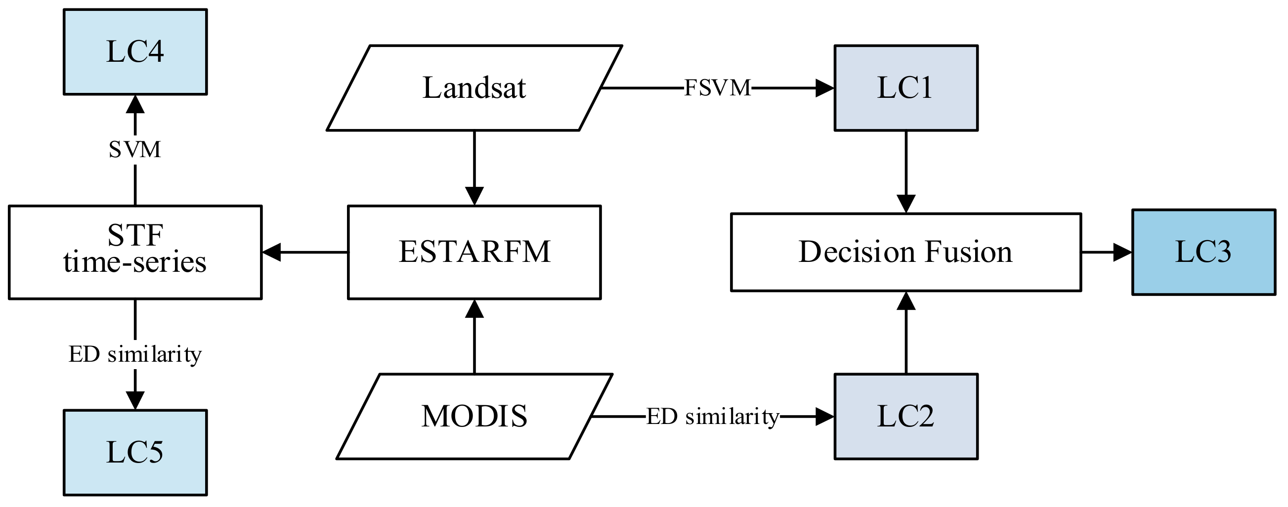
In these two experiments, the proposed method was compared with two single-source classification methods and two ESTARFM-based fusion methods. The workflow of the comparison experiment in two cases is shown in Figure 4. LC1 and LC2 are the classification results from Landsat and MODIS data using FSVM and ED similarity methods, respectively. LC3 is the fusion result of the PBF method. At the same time, the ESTARFM method [5] was also implemented for Landsat and MODIS data. The ESTARFM result is a time series of HSR data, which would be classified for LC4 and LC5 by SVM classifier and ED-similarity based classifier. The comparison and analyses of the five different classification results in each experiment will be displayed in Section 4. The following will be the materials of the two experiments, including the dataset and study area.

3.1. Comparisons on the Benchmark Dataset

3.1.1. Datasets Description

The robust benchmark STF datasets were developed to test different STF approaches [10]. There are three Landsat-MODIS datasets in the benchmark datasets. In this experiment, the AHB dataset was employed owing to its focus on phenological changes. The AHB dataset provides a benchmark dataset in rural areas, collected from Ar Horqin Banner (43.3619°N, 119.0375°E) located in the northeast of China. This area experienced significant phenological changes owing to the growth of crops and other kinds of vegetation.
In the AHB dataset, there were 27 pairs of cloud-free Landsat-MODIS images from 30 May 2013 (denoted as 2013/05/30) to 6 December 2018 (denoted as 2018/12/06). For details, the reader is referred to Ref. [10]. The Landsat-MODIS image pairs in 2018 were chosen in this experiment, which included seven pairs of the dates 2018/01/04, 2018/02/05, 2018/03/25, 2018/05/12, 2018/10/03, 2018/10/19 and 2018/12/06 with missing pairs in some months. Because the AHB area experienced significant phenological changes, it might seem difficult to reflect the important phenology variations by images with missing between May to October. Considering the AHB area did not undergo many land cover changes, the pairs of images in 2017 were used to make up for missing data of 2018. The entire time series of AHB dataset in this experiment are ten Landsat-MODIS image pairs in the dates of 2018/01/04, 2018/02/05, 2018/03/25, 2018/05/12, 2017/06/10, 2017/07/28, 2017/08/29, 2018/10/03, 2018/10/19 and 2018/12/06. The above dates can be abbreviated with mm/dd, such as 12/06 for 2018/12/06.

3.1.2. Preprocessing

In the AHB dataset, a sample of 175 points were selected for classification training (for 8 classes) and parameter estimation. A sample of 106 points were selected for accuracy assessment. Google Earth high-resolution images were referenced with sample points’ selection (including the above two samples), including construction area, two kinds of crops, slope field, wasteland, water, gobi, and grassland. The number of sample points per class was greater than 30.
The high-quality Landsat data are challenging to obtain in some regions. In this experiment, two pairs of Landsat-MODIS data were used for ESTARFM method inputs. The Landsat-MOIDS pairs of 2018/01/04 and 2018/05/12 were employed to predict HRS data in other dates, including 2018/02/05, 2018/03/25, 2017/06/10, 2017/07/28, 2017/08/29, 2018/10/03, 2018/10/19 and 2018/12/06. After ESTARFM fusion, we obtained a time series of high-spatial resolution data, which would be used as the input in the SVM classifier and ED-similarity based classifier to obtain the classification results. The two Landsat images of 2018/01/04 and 2018/05/12 were also employed for preclassification in the proposed method, as well as the corresponding ten MODIS images in 2018. The process and parameters of the developed PBF method are referred to in Section 2.3.2 and Section 2.3.3; the main parameters will also be displayed in Section 4.1.1. The following section will show the comparison results.

3.2. Application on a Large Area

3.2.1. Study Area

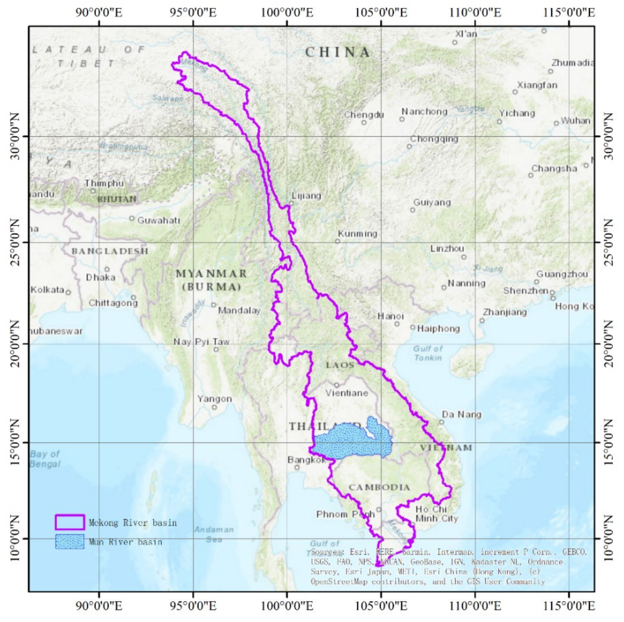
The Mun River Basin is located in the northeast of Thailand, between 101°30′–105°30′E and 14°–16°20′N (Figure 5). The Mun River is one of the Mekong River’s major tributaries. As the largest river on the Khorat Plateau and the second longest in Thailand, the river has a length of 673 km with a drainage area of about 70,500 km2. The area features a humid tropical monsoon climate with an annual temperature of 18 °C or greater, and an average annual precipitation of 1300~1500 mm. Crops are cultivated and harvested two or three times per year in many areas due to suitable hydrothermal conditions. The crop spectral characteristics can vary at different times and locations since the planting period is not limited by a fixed growing season. The basin is characterized by the medium landscape-level heterogeneity of land cover. The land cover categories include paddy rice, dry land, evergreen forest, deciduous forest, artificial forest, grassland, urban and construction land, wetland, and water.

3.2.2. Data and Preprocessing

The 2015 MOD09Q1 data were used in this study, which provided the surface reflectance values for MODIS imagery in bands 1 and 2 at a 250 m resolution. Each MOD09Q1 pixel contained the best possible L2G observation during 8 days and was selected based on favorable attributes such as high observation coverage and low view angle. The two MOD09Q1 bands were obtained for NDVI (normalized difference vegetation index) calculation.
Landsat 8 OLI data were obtained from the United States Geological Survey (USGS) website (https://earthexplorer.usgs.gov (accessed on 20 July 2021). This dataset consists of high-quality images that contain less than 10% cloud cover. The Landsat 8 satellite carries the operational land imager (OLI) and includes nine bands. The imagery features eight multispectral bands with a resolution of 30 m and a 15 m panchromatic band.
Sub-resolution changes may cause noise in the satellite time series due to atmospheric conditions and geometric errors produced by the sensors [53]. The adaptive S-G (Savitzky–Golay) filter in the TIMESAT software [54] was used to reduce noise in the MODIS NDVI time-series data. The TIMESAT software employs QA data for improved noise filtering. The QA data were decoded from the original HDF MODIS data using the LDOPE tool. Specifically, bit 2–3 “cloud state” was used as a reference weight for TIMESAT S-G filtering. In this study, the clear data (Bit Comb. 00) were weighted as 1, the cloudy data (Bit Comb. 01) were weighted as 0.5, and the mixed and unset data (Bit Comb. 10 and 11) were weighted as 0.1. A window size of four was used for the filter. The adaption strength was set as two, and the number of envelope iterations was set to three.
The Landsat 8 OLI image is a Level 1T product. The radiometric calibration and FLAASH model-based atmospheric correction were performed in ENVI 5.0 SP3 software. The Landsat 8 OLI data were then resampled to 25 m with the nearest-neighbor resampling technique. The sample points were categorized into five groups. Group 1 was used to estimate the areal proportion of each class. Group 2 was used for obtaining the reference NDVI time series of each class. Group 3 was used for supervised classification (FSVM) of the image objects produced by high-spatial-resolution data. Group 4 was used for the accuracy validation of preclassification results. Group 5 was used for the validation of the proposed fusion scheme. The points in group 1 were considered a union of groups 3, 4, and 5 because they were random samples. The number of sample points in group 1 was greater than 50 for each class. The points in group 2 mainly were pure-pixel sites that were carefully selected. The point labels were obtained through a field survey in 2016 and combined with the manual interpretation of high-resolution Google Earth imagery. There were 887 points in group 1, 120 points in group 2, 219 points in group 3, 329 points in group 4, and 339 points in group 5. The distribution of points and their labels are shown in Figure 6. Only group 1 and group 2 are shown here to briefly display the samples. The following section will display the fused map deduced from PBF.

4. Results

4.1. Fusion Results of the Benchmark Dataset

4.1.1. Main Parameters of PBF

According to the mentioned calculations of parameters in the PBF method, the following displays the main parameters.
  • Area proportion p w k for each class k
The p w k variable is the areal proportion of class k on the whole map estimated from sample points. The samples were selected randomly, and the proportion of each class sample represents the areal proportion with a 95% confidence interval. The results for p w k and the eight classes are listed in Table 1.
2.
Classification membership of MODIS data μ t k x and Landsat data μ s k x
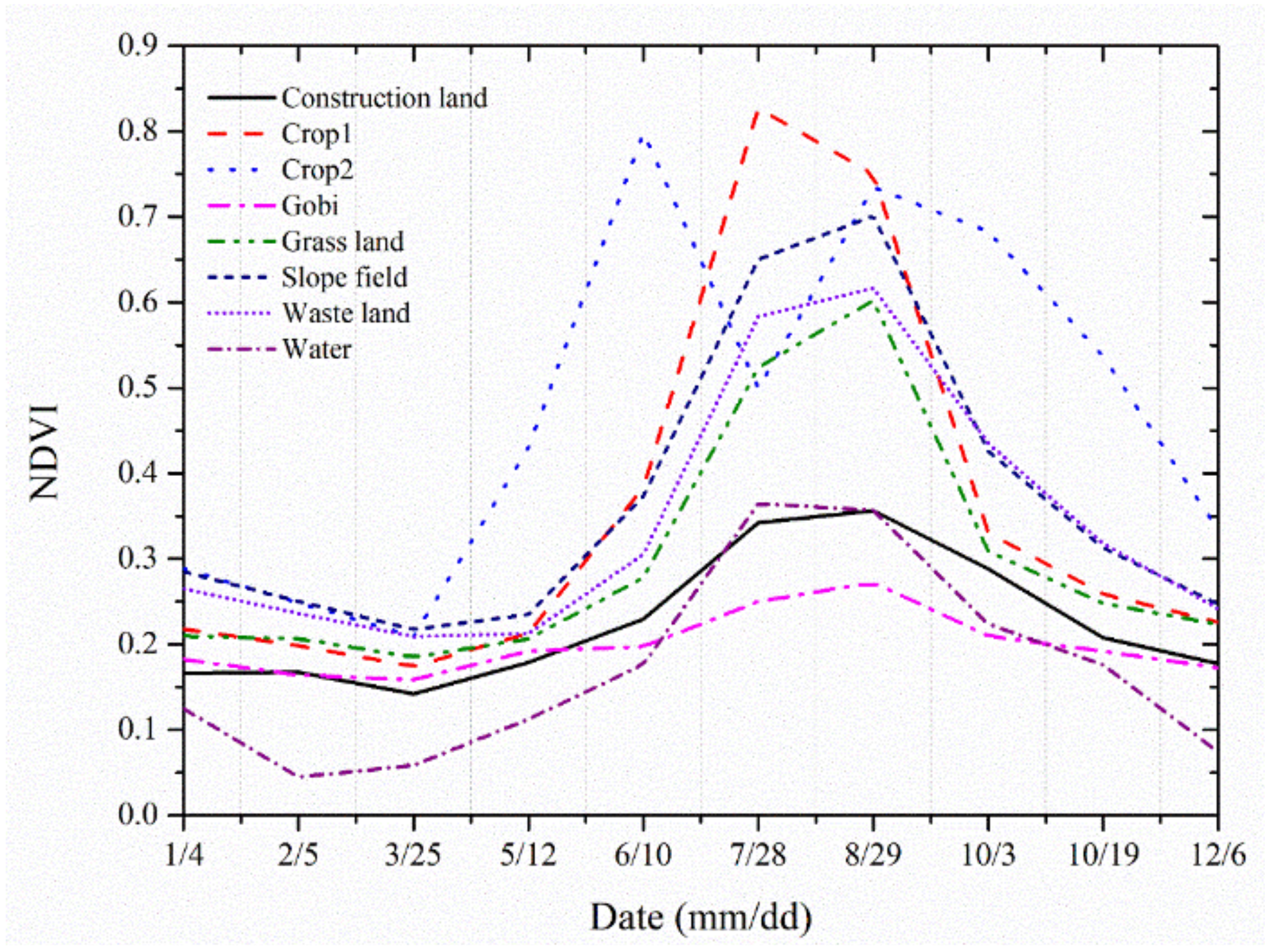
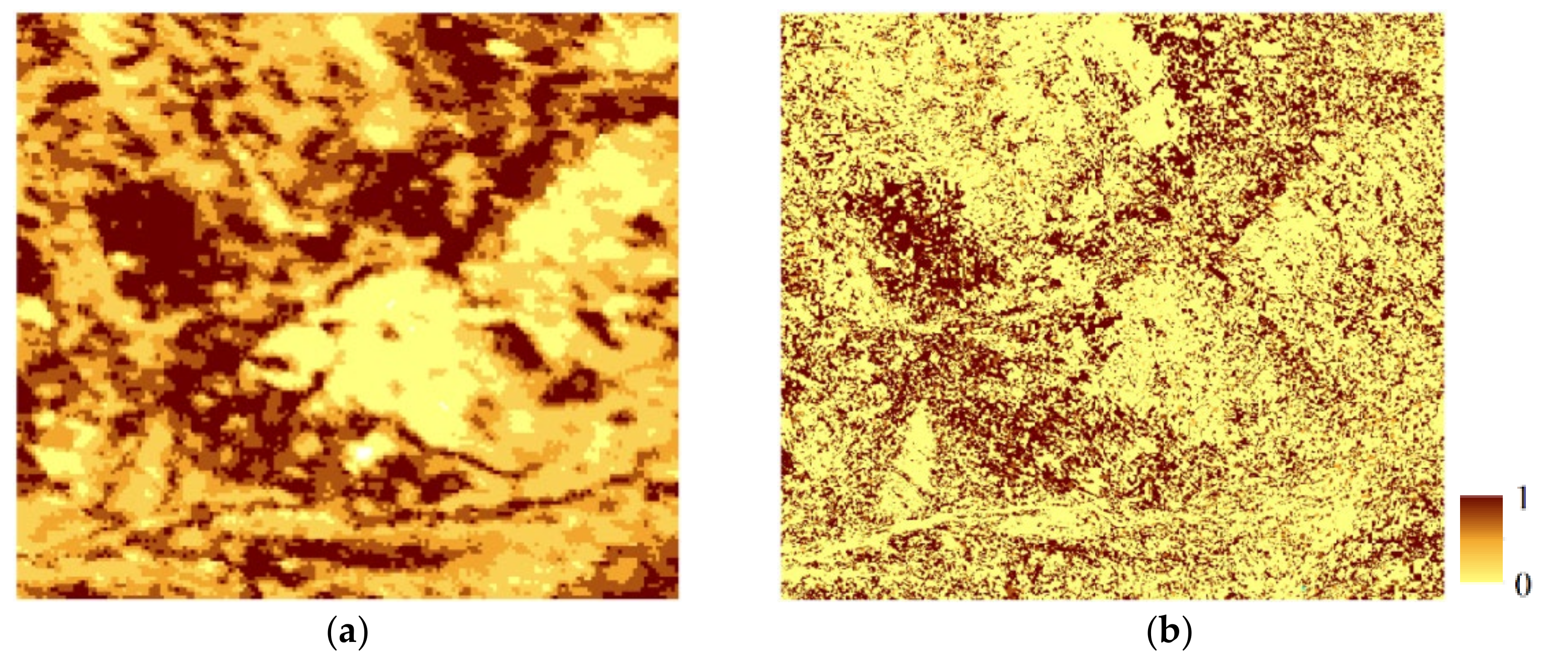
Following the fusion scheme, MODIS and Landsat data were segmented and classified. The reference NDVI curve of MODIS collected by samples is shown in Figure 7. The MODIS data were first classified using the ED similarity classifier. The image objects produced by the segmentation of Landsat pixels were classified using the FSVM classifier. The membership values μ t k x and μ s k x of land features were obtained for MODIS and Landsat imagery (Figure 8). In Figure 8, the membership values for only grassland are displayed via MODIS and Landsat imagery for succinctness.
3.
Classification accuracy and uncertainty assessment parameters
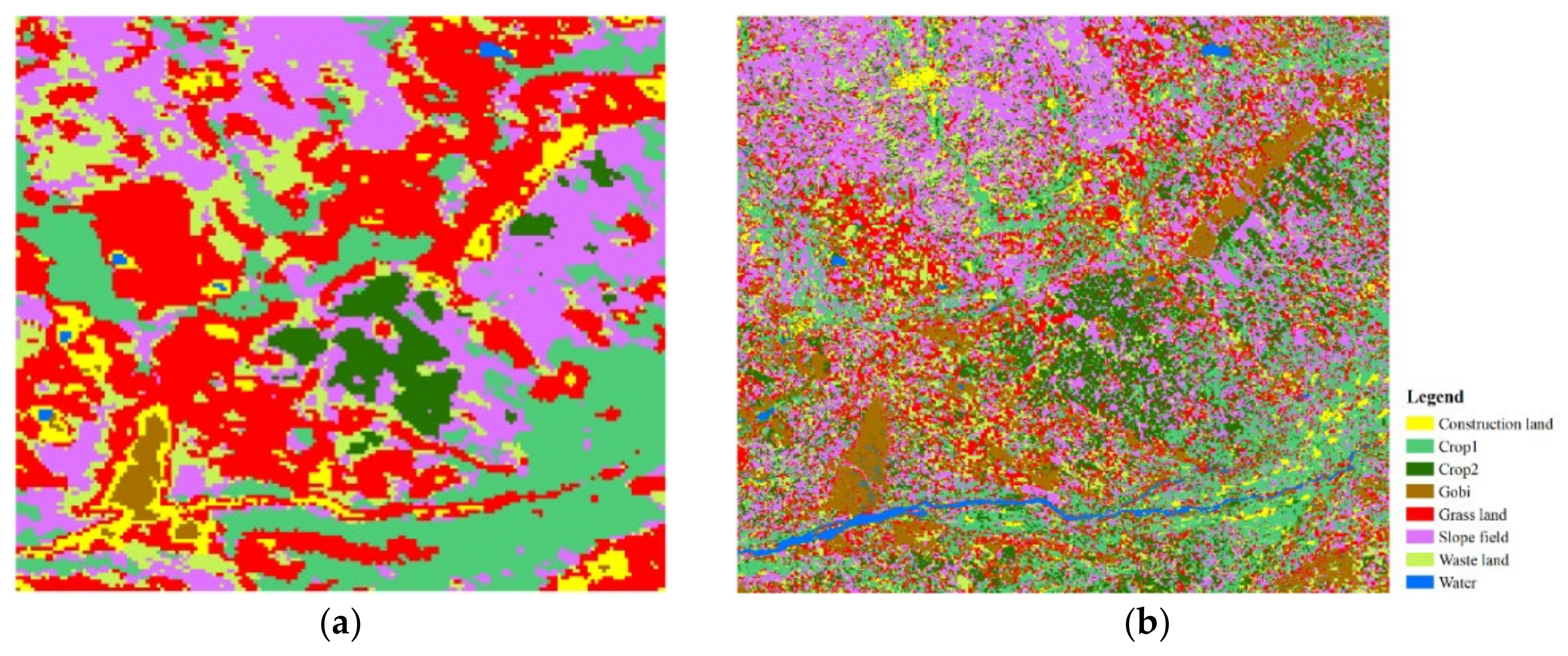
According to the membership values shown in Figure 8, the class with the highest membership value was considered the final class type in the classification results. The classification results for the two datasets are shown in Figure 9.
The land-cover accuracy for the preclassification results was assessed using 106 test samples and a confusion matrix. The two per-class accuracies f t k x and f s k x are as shown in Table 2. The classification accuracy for the graded area in the MODIS time-series data was obtained using Equation (13). According to samples, A d | d = 1 , 2 , 3 , , 10 was [0.25, 0.33, 0.45, 0.62, 0.50, 0.25, 0.46, 0.25, 0.66, 0.71]. Then, f   t k x was obtained in Table 3 for eight classes. The weights of memberships ω t and ω s can be obtained from Equation (15), and the class allocation of uncertainty θ t and θ s can be calculated based on membership and its weight using Equation (16). The weight of membership of MODIS data was found to be relatively low, and the weight of membership of Landsat data was relatively high, each to a great extent (as shown in Figure A3). MODIS data were found to contain more mixed pixels, which caused high fuzziness within the pixels. The fine-resolution Landsat imagery contained fewer mixed pixels, which resulted in low fuzziness. Now, we have obtained all the parameters for PBF of Equation (9). The fusion result will be shown in the next subsection.

4.1.2. Fusion and Classification Results of the ESTARFM and PBF Methods

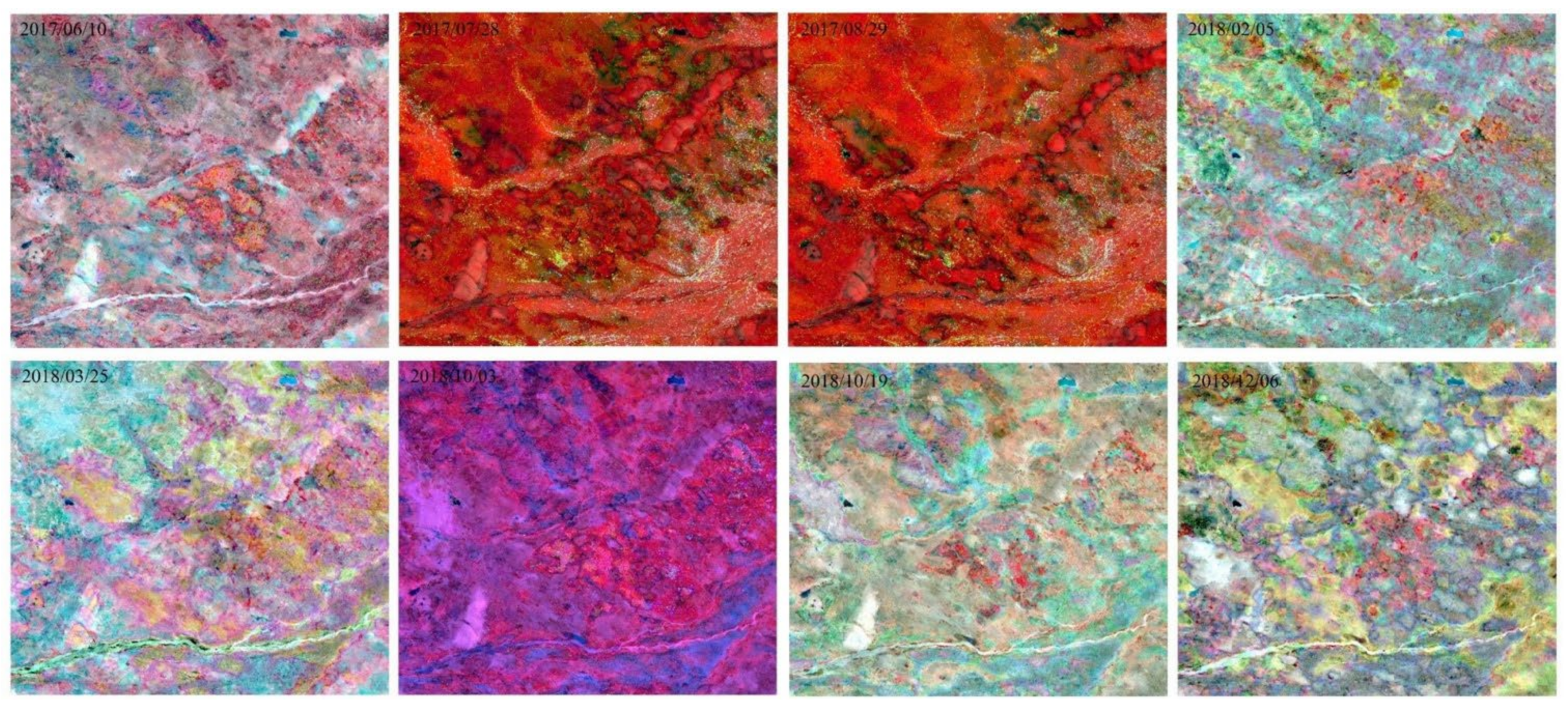
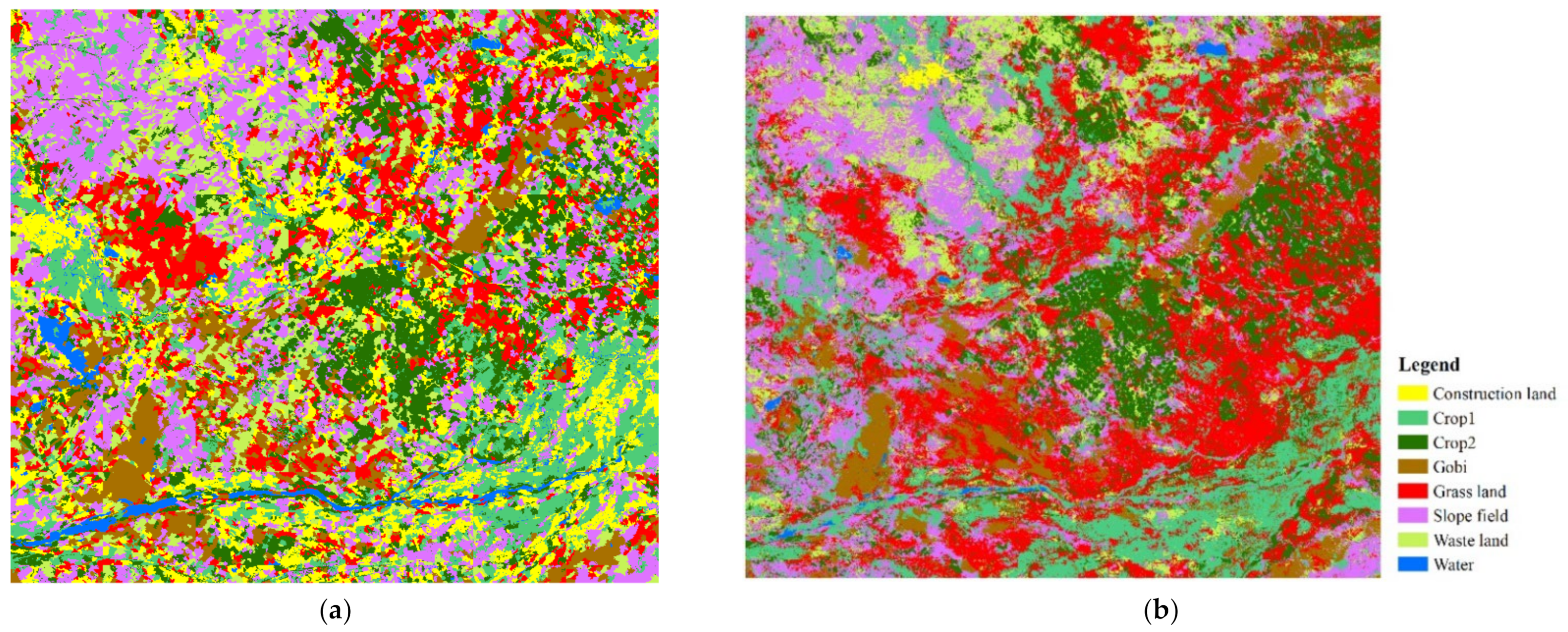
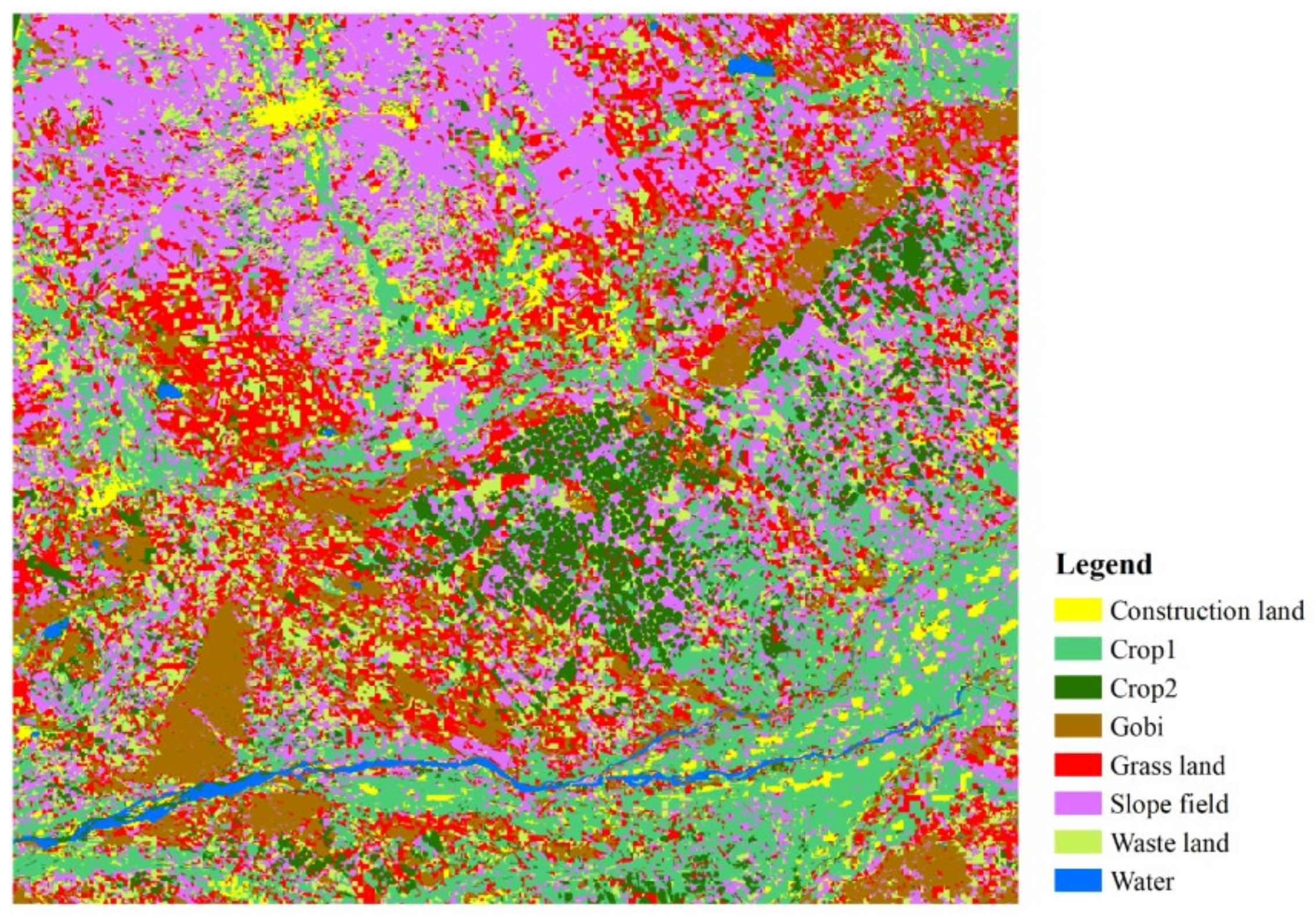
The fusion results of ESTARFM are shown in Figure 10, using the image pairs of 2018/01/04 and 2018/05/12 to predict other dates. After fusion, the HSR time-series data were applied in the land cover classification. Both SVM and ED-similarity measures were used for land cover classification. The land cover maps LC4 and LC5 are shown in Figure 11. After obtaining all the parameters for the PBF method, we can obtain the decision fusion result of the land cover data, which is shown in Figure 12.

4.1.3. Accuracy Assessments and Comparisons

The five classification results were validated using the 106 test samples, including LC1 and LC2 based on the single-source data, LC3 of the PBF method, as well as LC4 and LC5 from the ESTARFM. Table 4 shows the class-wise accuracy comparison of the Landsat FSVM classification result, MODIS ED-similarity measure classification result, PBF result, and time-series data classification results predicted by the ESTARFM method, and they are classified by both the SVM and ED-similarity measure.
As shown in Table 4, the accuracy of the PBF method achieved better overall accuracy as well as class-wise accuracy. The overall accuracy of PBF rose by an average of 41.7% compared with LC1 and LC2, and an average of 21.2% compared with LC4 and LC5. The overall accuracy improvements in PBF were 8.13%, 75.29%, 3.62%, and 38.73% for other land cover classification results, respectively. LC4 derived from the ESTARFM method that was classified by the SVM classifier also achieves higher accuracy than the Landsat and MODIS classification accuracy. ESTARFM-based LC5, classified by using ED-similarity and MODIS-based LC2, achieved worse outcomes. The two worst performances were all from time-series similarity-based classification as the last step, which might be influenced by the reference NDVI time-series curves. The class accuracy of construction land and water were both high in the case of LC1, LC3 and LC4, owing to their highly recognizable characteristics. The difference between these two land types might be very confusing in classification. The waste and grasslands were usually smaller in the area where the fusion with coarse MODIS could not play the role or not be used well, also resulting in a marginal impact on accuracy improvement.

4.2. Fusion Result of the Mun River Basin

4.2.1. Classification Results and Comparison of Different Methods

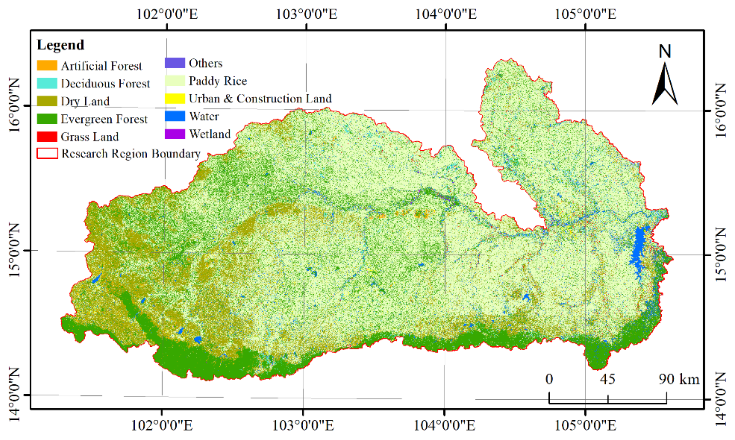
The developed PBF approach was also applied in the Mun River Basin to verify its practical value for large areas. The land cover maps LC4 and LC5 based on ESTARFM are shown in Figure 13. The process of obtaining the main parameters in PBF is identical to Section 4.1.1, and is presented in the Appendix A. The probability for each class was calculated. Figure 14 displays the inferred probability (i.e., posterior probability) of the selected three classes in the PBF method. The final fusion result was calculated using the posterior probability. Classes with the maximum probability were chosen as the final class for the fusion map. The final fusion map of PBF is shown in Figure 15.
Group 5 was used to validate the accuracy of the classification map after obtaining the fusion result. The class-wise accuracy and producer’s accuracy were compared with the fuzzy classification results using single-source data and multiple-source data. The individual classification accuracy values of each class were evaluated using Equation (12). This included the MODIS, Landsat, and two ESTARFM-based classification results, as shown in Table 5. As seen in Table 5, the overall accuracy of fusion data was higher than the individual classification results for MODIS and Landsat data and fusion classification results based on ESTARFM. It is clear that with the relatively high overall accuracy of 57.23%, the PBF method produced the greatest performance for the classification. Although none of the five classification results had an overall accuracy of more than 60%, the performance of the PBF method improved on average by 13.93% than the two single-source classifications, and 6.08% than the two ESTARFM-based classifications. The overall accuracy of PBF in the Mun River Basin rose by an average of 10% on the whole. The overall accuracy cases in the five classification results might be caused by the complex heterogeneity of the large region. The classification accuracy for paddy rice and dry land, which occupied more than 72% of the total area, was greatly improved and thus improved the overall accuracy. Additionally, the Bayesian decision fusion method also improved the classification accuracy for wetlands. The fusion results for deciduous forests, grasslands, urban and construction land, and water bodies were all greater than the classification accuracies produced by one of Landsat and MODIS. However, the classification results for artificial forests, evergreen forests, and other classes decreased in accuracy. The classification accuracy for artificial forests and the “others” class was equal to zero after fusion, which was not a good indication of the fusion scheme’s performance. This might be attributable to the relatively low areal proportion of the “others” class and artificial forests, which only occupied 1.52% of the area. On the one hand, the classification results for objects with smaller areas were less reliable when using high-temporal-resolution data, which might lead to their omission from the fusion map. On the other hand, the number of verification samples of these classes with low areal proportion were much lower than other classes. It also affected the corresponding classification accuracy, which might result in zero. As a result, the poor performance of the fusion data for the two types did not significantly impact the overall accuracy. Other classes, such as evergreen forests, also featured a decline in accuracy after fusion. Most of the class accuracies were observed to improve the accuracy of the data source. The accuracy for dry lands, paddy rice fields, and wetlands, as well as the overall accuracy, also improved when both data sources were considered.

4.2.2. Error Matrix Analysis in PBF

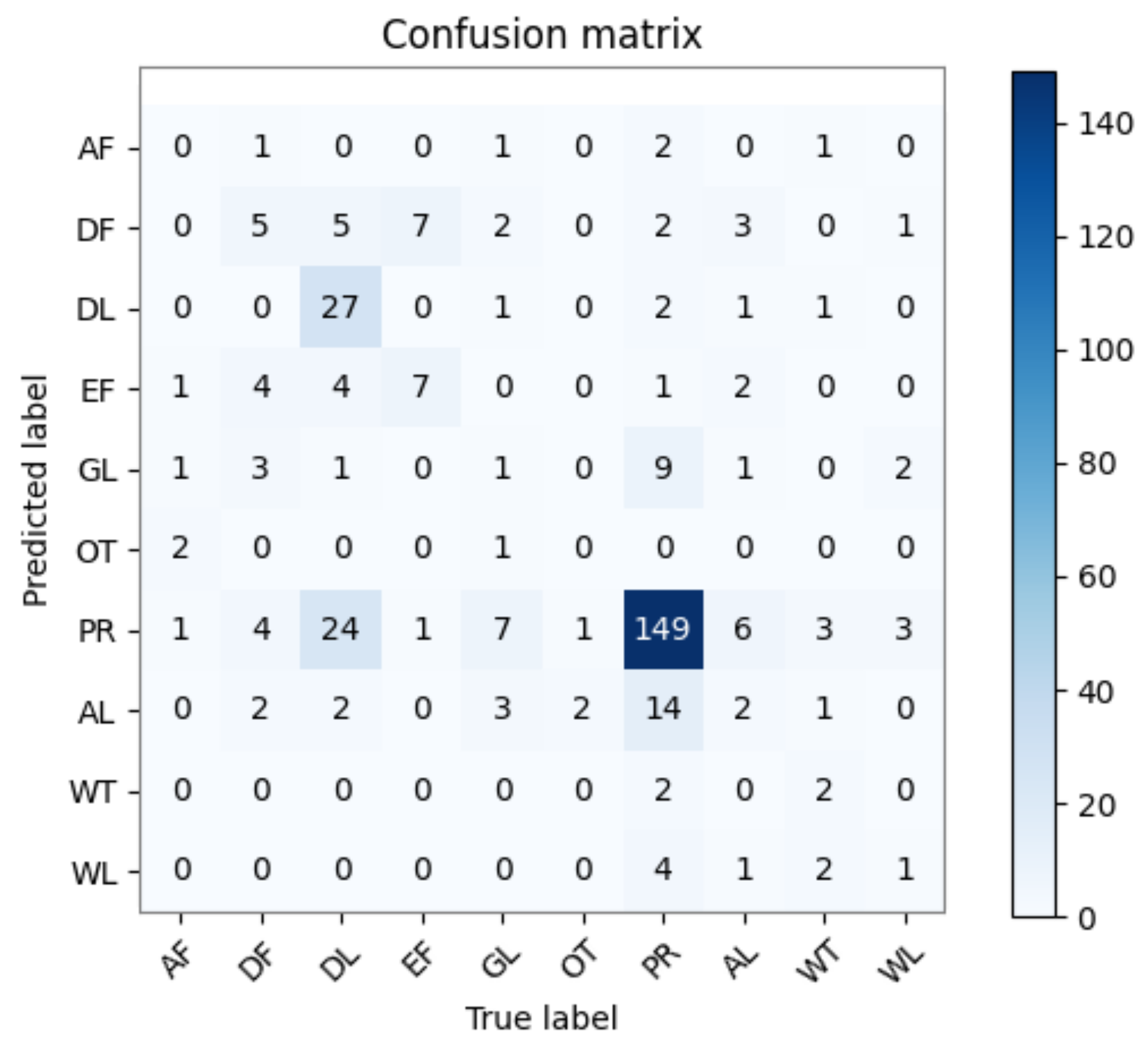
The PBF method showed noticeable improvements in the overall accuracy in the application experiments. Because of the complex heterogeneity in the Mun River Basin, the five classification results had overall accuracy values of no more than 60%. The highest of overall accuracy was 57.23% derived from the proposed method. In total, 339 sample points were validated on the fusion map. The visualized confusion matrix of the PBF result is shown in Figure 16. We analyzed the reason for this result in the following.
The artificial forest accuracy was zero. Five samples were labeled as artificial forests, one of the points was classified as evergreen forest, one was classified as grassland, two were classified as “others”, and the last point was classified as paddy rice. It is understandable that artificial land was misclassified as evergreen forest and grassland because the spectral reflectance of grown artificial forests can be similar to deciduous forests. Furthermore, the spectral reflectance of immature artificial forests can be similar to that of grassland. However, the spectral reflectance was not similar to the “others” and paddy rice classes. Some of the sample points were also misclassified as paddy rice.
In total, nineteen samples were labeled as deciduous forests, five of the points were correctly classified as deciduous forests, and one point was misclassified as an artificial forest. Moreover, four points were misclassified as evergreen forest, and three were misclassified as grassland. This is understandable since forests and grasslands are spectrally similar. However, four points were classified as paddy rice, and two points were classified as urban and construction land.
In all, 27 out of 63 sample points were correctly classified as dry land. One of the points was classified as grassland, which is unsurprising since grass tends to grow when the land is in a fallow period. Two points were classified as urban and construction land, which is also understandable because urban and construction land includes tiny villages and scattered settlements. The mixed-pixel effects can lead to the misclassification of dry land. Five points were classified as deciduous forests, four points were classified as evergreen forests, and twenty-four points were classified as paddy rice. The misclassification between dry land and paddy rice is due to their similar spectral characteristics.
Overall, seven sample points were correctly classified as evergreen forests; however, seven points were misclassified as deciduous forests because the spectral characteristics of deciduous forests are similar to evergreen forests. One point was classified as paddy rice. Only one in sixteen points was correctly classified as grassland, and the others were mainly classified as paddy rice fields and forests. None of the other pixels were correctly classified, and misclassified as paddy rice and urban and construction land.
In all, 149 out of 185 paddy rice sample points were correctly classified. Nineteen points were misclassified as “others” and urban and construction land, which was caused by the mixed-pixel effect. Two points were classified as dry land, which can be very similar to paddy rice when flooded. Five points were misclassified as forests, nine misclassified as grassland, and fourteen classified as urban and construction land. Urban and construction land, wetlands, and water bodies mainly were misclassified as paddy rice and featured low classification accuracy.

5. Discussion

In this paper, a Bayesian-fusion-theory-based approach was proposed to fuse the fuzzy classification results produced by high-to-medium-resolution time-series remote sensing data. In order to further discuss the performance of the developed PBF method, we analyzed the errors from the preclassification results of the above application study. We also further validated the effectiveness and discussed possible extension of this approach, which also, respectively, made a comparison in the Mun River Basin.

5.1. Errors from Preclassification Results

The results produced by the PBF method were theoretically rational. The decision fusion strategy is based on a combination of a priori probability and conditional probability. Both the a priori probability and conditional probability were low for these classes with low areal proportion in the fusion process. Therefore, a class will have a higher probability of decision fusion if it occupies a larger area. This strategy increases the possibility of the pixel being classified with more extensive areas. The method is beneficial since it can increase the overall accuracy of the classification map. However, the technique is also disadvantageous since it can result in losing some map details, such as the relatively poor classification performance of the low-areal-proportion class, which could be considered by increasing the weights of classification for small patches under certain conditions in future research. Taking the application study on the Mun River Basin as an example, the fusion results are analyzed, and a reason is provided for the decrease in the individual class accuracy in this subsection.
Some of the unreasonable classification results were selected for analysis based on the individual data sources, listed in Table 6. As shown in Table 6, most misclassifications occurred in the preclassification process. The training strategy of decision-level fusion approaches mainly occurred in preclassified processes [31,55]. The parameters in PBF would be directly calculated by preclassified results and specific equations mentioned in Section 2.3.3. The misclassified pixels in MODIS and Landsat data would influence every fusion step that follows, such as the memberships of preclassification imagery at close to “true” value, which led to misclassification in the fusion results of PBF. Therefore, the incorrect classification of preclassification results was a major cause of misclassification in the fusion map. Additionally, in the case of the high memberships for pixels classified correctly in MODIS and Landsat, the PBF method would also be possible to derive misclassification, such as PR example in Table 6. The corresponding membership of another class (i.e., not PR) might also be a high value, enhancing the uncertainty of the classification result. As mentioned above, the membership set (0.1 0.9 0.1) is more “reliable” than set (0.9 0.8 0.85). The fusion strategy in PBF doesn’t merely rely on the classification memberships; also includes the uncertainty of classified results. The principle of the decision fusion scheme makes it possible to choose preclassification algorithms freely [56]. Therefore, fusion results can be improved by improving the performance of preclassifiers [57].

5.2. Comparison with a Decision Fusion Method

The classification accuracy produced by the PBF method was higher than the individual classification accuracy for MODIS and Landsat data, as well as the ESTARFM-based classifications. A comparison experiment was conducted to further evaluate the effectiveness of the proposed method. The PBF results were compared with a compromise-based decision fusion (CBDF) method proposed by Fauvel et al., (2006) [36]. Based on the spatial unification mentioned in Section 2.3.3, the key difference between these two methods lies in the fusion step. For CBDF method, without the prior probability, Equation (9) can be rewritten as μ k x = max min ω t x μ t k x ,   f   t k x , min ω s x μ s k x ,   f s k x . The decision fusion results of CBDF can be obtained as shown in Figure 17, then was validated using the samples of group 5. Table 7 displays the comparison among different classification accuracy from Landsat, MODIS, CBDF and PBF.
As shown in Table 7, CBDF was observed to produce higher overall classification accuracy compared with the Landsat and MODIS classification results. However, in terms of class-wise classification accuracy, the compromise fusion strategy’s performance was similar to PBF. The classification accuracy for dry land and paddy rice was observed to improve, but this was not necessarily the case for other class accuracies. The PBF strategy achieved a higher overall accuracy compared to CBDF strategy. In terms of class-wise classification accuracy, PBF generally performed better than CBDF. This illustrates that PBF can perform better than CBDF strategy, which does not consider the prior probability in the fusion process. Moreover, the proposed method synthesizes the prior probability, the class allocation of uncertainty, and the class-wise classification accuracy of each data source.

5.3. Possible Improvement

The improvement in overall accuracy produced by the PBF scheme is not coincidental. The overall accuracy can be improved because the fusion scheme has the highest probability for single objects and produces a classification map with a higher probability of correct classes [9]. However, this scheme can result in the loss of detailed information in the fusion map, as shown in the results. A strategy was tried to retain the individual classification results with a high probability of being correct in the final fusion [58]. The strategy was to combine the class-wise and class allocation of uncertainty with the product rule rather than the conjunctive combination rule in Equation (7), which can be rewritten as μ k x p w k × ω t x μ t k x × f   t k x × ω s x μ s k x × f s k x . It was speculated that the result might improve due to the preservation of single data results with high class-wise and local accuracy. Figure 18 displays the fusion map using the product combination rule. Group 5 was also used to validate the results (Table 8). The classification accuracy was obtained using the fusion strategy based on Bayesian theory. The product combination rule was selected as the combination rule for conditional probability.
In Table 8, the overall accuracy produced by the product combination rule exceeded the accuracy delivered by the conjunctive combination rule. However, the two rules did not feature a significant difference in performance for individual classes. The accuracy values for the artificial forest, “others”, and wetland classes were equal to zero. The main difference was that the product combination rule improved the accuracy of evergreen forests; however, its accuracy was lower than that produced by the MODIS data. This result indicates that the product rule might perform better than the conjunctive rule in terms of overall accuracy.
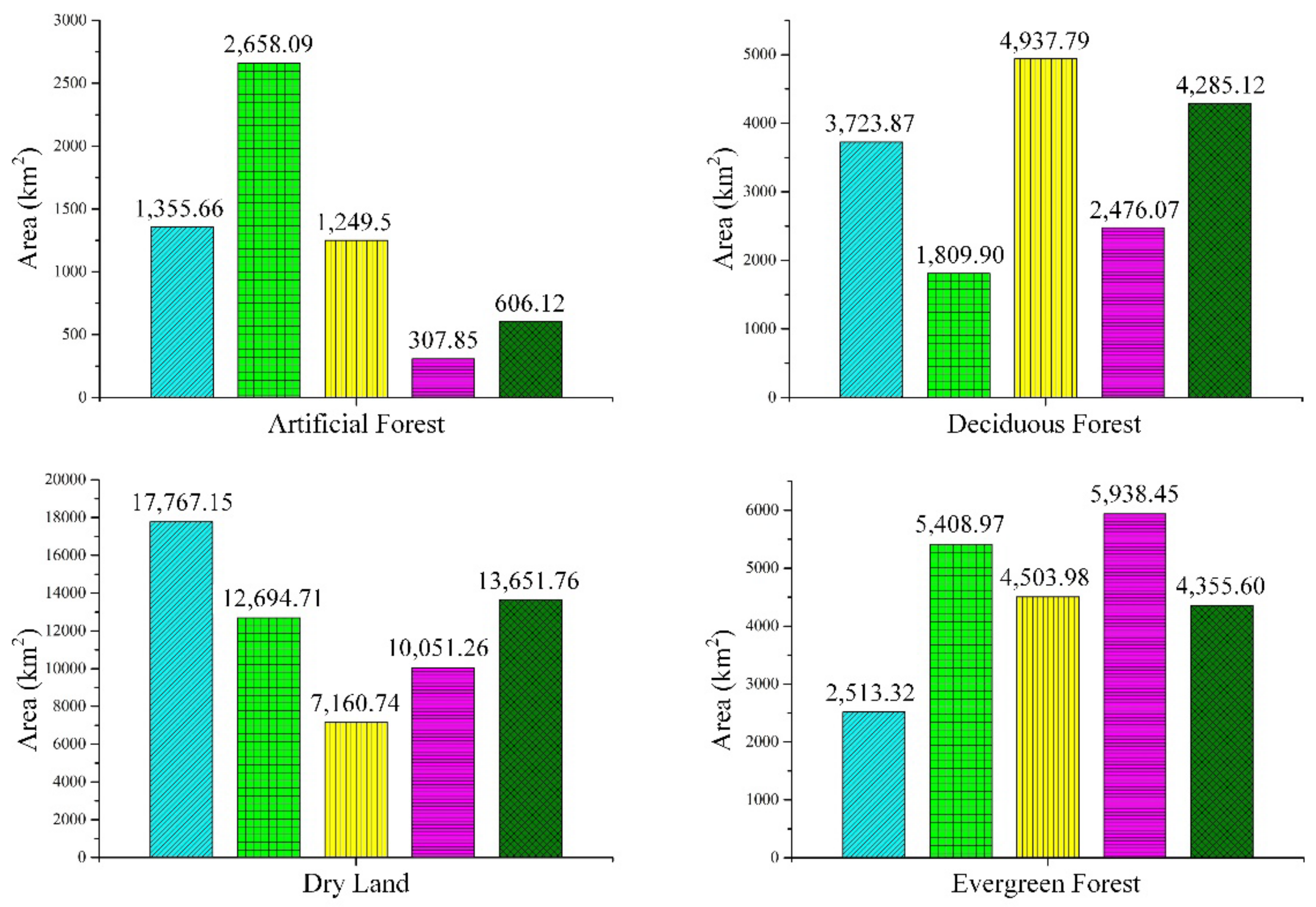
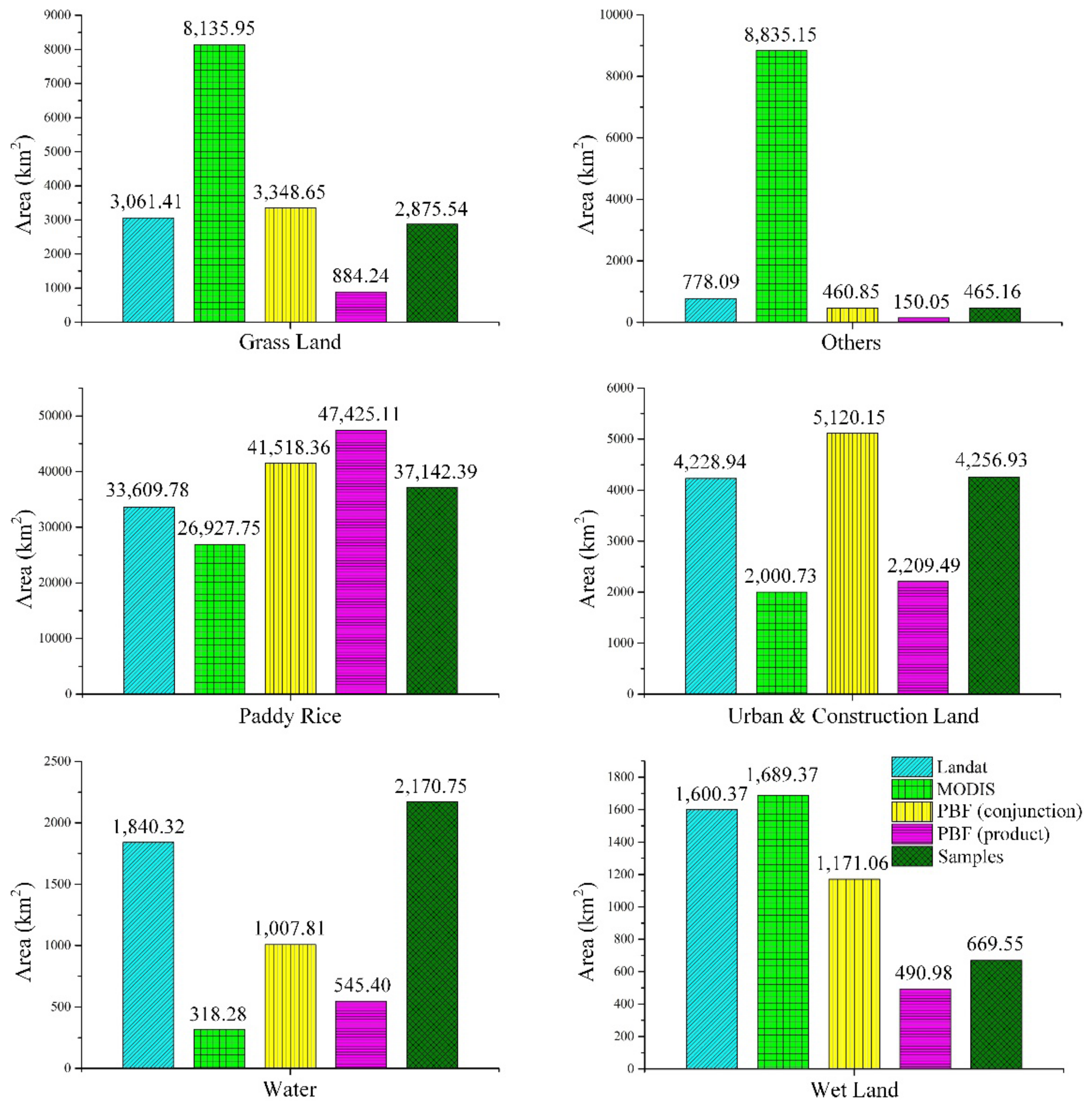
Moreover, the original classification accuracy for Landsat and MODIS imagery was low for classes such as artificial forest, grassland, “others”, and wetland. Moreover, the areal proportion of these classes was also relatively small. Therefore, both the prior probability and conditional probability were low for these classes in the fusion process, which led to their omission from the fusion map. Figure 19 displays the total area of each class estimated by samples and four land cover classifications. The four classification results were derived from two single-source methods and two PBF methods with different combination rule. The estimated true areal proportion of paddy rice and dry lands were 52.7% and 19.37% by using samples. The overall accuracy is 52.7% if all pixels are classified as paddy rice. The PBF (product combination) result classified more paddy rice than other methods and data. However, apart from evergreen forests, the method also classified less land cover than other methods.

6. Conclusions

In this paper, a decision fusion algorithm was proposed based on Bayesian decision theory. The PBF method was developed using a combination of classifiers to fuse high-spatial-resolution and high-temporal-resolution data to improve classification accuracy. The decision fusion performance was enhanced by combining the class allocation of preclassifier uncertainty and the preclassification results based on conditional probability. A comparison experiment was conducted with the STF baseline method on a benchmark dataset. It showed that under the circumstance of the limited number of high-quality Landsat data available, the PBF method can achieve better classification accuracy than the STF-fusion baseline method when the fused spatiotemporal data are classified by the SVM and ED-similarity methods. This fusion scheme was also applied to combine classification information from MODIS time series and Landsat imagery in a large area. The results also show that the proposed method can improve the overall accuracy of classification maps compared with a single data source and STF-fusion baseline method, which rose by an average of 10% in the Mun River basin land cover mapping. This approach confirmed that the statistical fusion approach is a helpful tool for integrating information provided by high-temporal-resolution and high-spatial-resolution remote sensing data. The potential analysis shows that the PBF method is a promising way to integrate multisensor information and improve the overall accuracy of classification maps. Furthermore, the proposed fusion scheme is not restricted to optical remote sensing images, and can also be used to combine multisource heterogeneous sensor information.

Author Contributions

Conceptualization, X.G., Y.J. (Yan Jin) and Y.G.; methodology, Y.J. (Yan Jin) and X.G.; software, X.G. and Y.J. (Yan Jin); validation, X.G.; formal analysis, X.G. and Y.J. (Yan Jia); investigation, X.G.; resources, Y.G.; data curation, X.G.; writing—original draft preparation, X.G. and Y.J. (Yan Jin); writing—review and editing, Y.J. (Yan Jin), X.G. and W.L.; visualization, Y.J. (Yan Jia), X.G. and W.L.; supervision, Y.J. (Yan Jin); project administration, Y.J. (Yan Jin); funding acquisition, Y.G. All authors have read and agreed to the published version of the manuscript.

Funding

This work was supported in part by the National Natural Science Foundation of China under Grant 42001332, the Strategic Priority Research Program of Chinese Academy of Sciences under Grant XDA 20030302, the Natural Science Research of Jiangsu Higher Education Institutions of China under Grant 20KJB170012, the National Natural Science Foundation of China under Grant 41725006, Grant 42130508, Grant 42001375, Grant 42071414 and Grant 41901309, the Natural Science Foundation of Jiangsu Province under Grant BK20191384, and the Scientific Research Fund of Nanjing University of Posts and Telecommunications under NUPTSF Grant NY219035.

Institutional Review Board Statement

Not applicable.

Informed Consent Statement

Not applicable.

Data Availability Statement

Not applicable.

Acknowledgments

The authors would like to thank all data producers.

Conflicts of Interest

The authors declare no conflict of interest.

Appendix A

The access to the parameters in the PFB method is described in Section 2.3, and the following displays the main parameters for the application of the Mun River Basin.
  • Area proportion p w k for each class k
The p w k variable is the areal proportion of class k on the whole map estimated from group 1. The results for p w k with the confidence interval and the ten classes are listed in Table A1.
Table A1. Area proportion of each class estimated by group 1 in the Mun River Basin.
Class (k) p w k   % Confidence Interval (95% Level)
Grass Land4.08[3.958, 4.202]
Evergreen Forest6.18[6.027, 6.333]
Urban and Construction Land6.04[6.007, 6.073]
Dry Land19.37[18.542, 20.198]
Deciduous Forest6.08[5.882, 6.278]
Others0.66[0.648, 0.672]
Artificial Forest0.86[0.840, 0.880]
Wetland0.95[0.934, 0.966]
Water3.08[3.001, 3.159]
Paddy Rice52.70[51.021, 54.379]
2.
Classification membership of MODIS data μ t k x and Landsat data μ s k x
The membership values of land features were obtained for MODIS and Landsat imagery (Figure A1). In Figure A1, the membership values for only three classes are displayed via MODIS and Landsat imagery for succinctness.
Figure A1. Memberships of three selected land covers from MODIS and Landsat data in the Mun River Basin. The membership value is between 0 and 1.
Remotesensing 14 06003 g0a1
3.
Classification accuracy and uncertainty assessment parameters
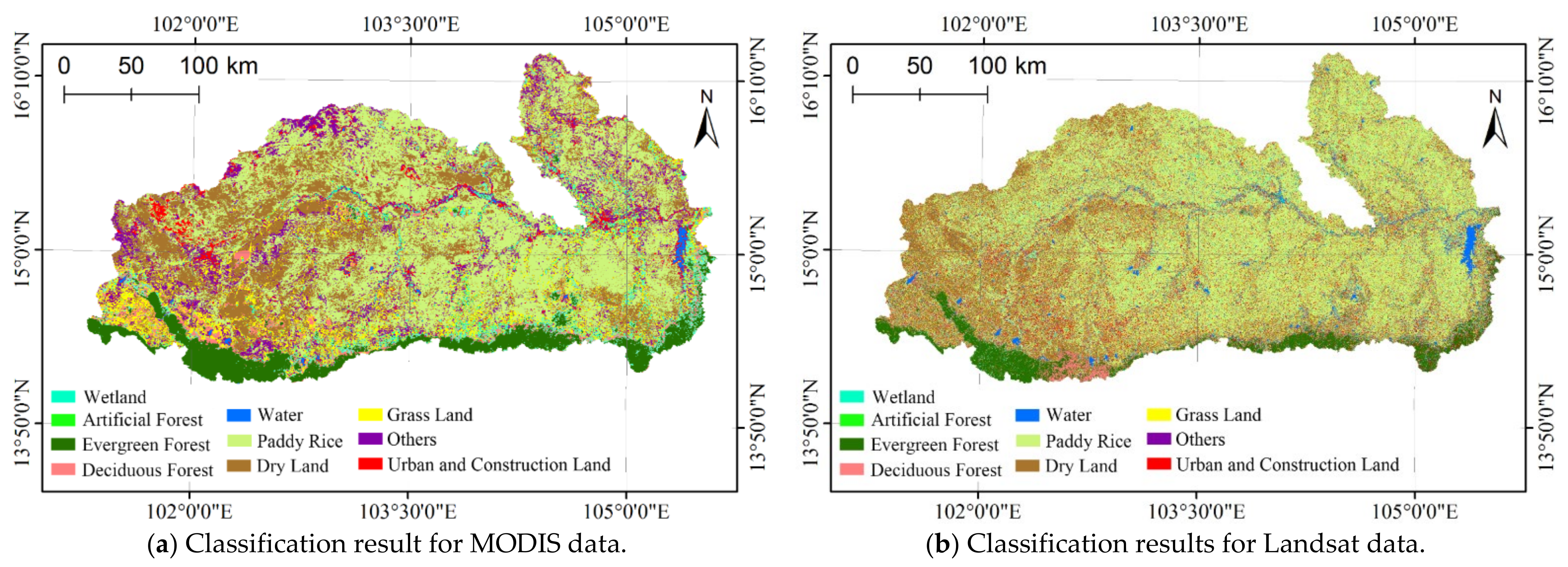
The classification results for the two datasets are shown in Figure A2. The land-cover accuracy for the preclassification results was assessed using group 4 and a confusion matrix. Class-wise accuracy is as shown in Table A2. According to group 4, A p | p = 1 , 2 , 3 , , 10 was [0.42, 0.43, 0.45, 0.46, 0.47, 0.60, 0.59, 0.52, 0.69, 0.71]. Then, f   t k x was obtained in Table A3 for ten classes. The weights of memberships ω t and ω s were obtained based on the fuzziness of membership, shown in Figure A3. The class allocation of uncertainty θ t and θ s can be calculated based on membership and its weight using Equation (16). After obtaining the preclassification results and the class-wise and class allocation of uncertainty, the fusion map derived from PBF was achieved and shown in Section 4.2.
Figure A2. Classification results for (a) MODIS and (b) Landsat data in the Mun River Basin.
Remotesensing 14 06003 g0a2
Table A2. Class-wise classification accuracy for Landsat and MODIS data in the Mun River Basin.
Class-Wise Accuracy
(Landsat)
Class-Wise Accuracy
(MODIS)
Grass Land0.030.08
Evergreen Forest0.560.79
Urban and Construction Land0.210.09
Dry Land0.410.31
Deciduous Forest0.230.26
Others0.060.01
Artificial Forest0.100.08
Wetland0.050.11
Water0.320.24
Paddy Rice0.730.73
Table A3. Class and area group-wise classification accuracy for MODIS imagery in the Mun River Basin.
GS 1EF 2AL 3DL 4DF 5OT 6AF 7WL 8WT 9PR 10
0–100.070.660.070.250.220.000.070.090.200.61
0–200.070.650.070.250.220.000.070.090.200.60
20–300.070.690.080.270.230.000.070.100.210.64
30–400.080.740.080.290.240.000.070.100.220.68
40–500.080.740.080.290.240.000.070.100.220.68
50–600.100.940.100.370.310.010.100.130.280.87
60–700.100.910.100.350.300.010.090.130.270.84
70–800.090.810.090.320.270.010.080.110.240.75
80–900.111.080.120.420.360.010.110.150.321.00
90–1000.121.110.120.430.360.010.110.150.331.02
1 GS—Grass Land. 2 EF—Evergreen Forest. 3 AL—Urban and Construction Land (Artificial Land). 4 DL—Dry Land. 5 DF—Deciduous Forest. 6 OT—Others. 7 AF—Artificial Forest. 8 WL—Wetland. 9 WT—Water. 10 PR—Paddy Rice.
Figure A3. The weight of class membership for (a) MODIS and (b) Landsat data.
Remotesensing 14 06003 g0a3

References

  1. Ma, L.; Li, M.; Ma, X.; Cheng, L.; Du, P.; Liu, Y. A Review of Supervised Object-based Land-cover Image Classification. ISPRS J. Photogramm. 2017, 130, 277–293. [Google Scholar] [CrossRef]
  2. Gómez, C.; White, J.C.; Wulder, M.A. Optical Remotely Sensed Time Series Data for Land Cover Classification: A Review. ISPRS J. Photogramm. 2016, 116, 55–72. [Google Scholar] [CrossRef] [Green Version]
  3. Löw, F.; Conrad, C.; Michel, U. Decision Fusion and Non-parametric Classifiers for Land Use Mapping Using Multi-temporal RapidEye Data. ISPRS J. Photogramm. 2015, 108, 191–204. [Google Scholar] [CrossRef]
  4. Chen, B.; Huang, B.; Xu, B. Multi-source Remotely Sensed Data Fusion for Improving Land Cover Classification. ISPRS J. Photogramm. 2017, 124, 27–39. [Google Scholar] [CrossRef]
  5. Zhu, X.; Chen, J.; Gao, F.; Chen, X.; Masek, J.G. An Enhanced Spatial and Temporal Adaptive Reflectance Fusion Model for Complex Heterogeneous Regions. Remote Sens. Environ. 2010, 114, 2610–2623. [Google Scholar] [CrossRef]
  6. Markham, B.L.; Storey, J.C.; Williams, D.L.; Irons, J.R. Landsat Sensor Performance: History and Current Status. IEEE Trans. Geosci. Remote Sens. 2004, 42, 2691–2694. [Google Scholar] [CrossRef]
  7. Miettinen, J.; Stibig, H.-J.; Achard, F. Remote Sensing of Forest Degradation in Southeast Asia—Aiming for A Regional View Through 5–30 m Satellite Data. Glob. Ecol. Conserv. 2014, 2, 24–36. [Google Scholar] [CrossRef]
  8. Tarnavsky, E.; Garrigues, S.; Brown, M.E. Multiscale Geostatistical Analysis of AVHRR, SPOT-VGT, and MODIS Global NDVI Products. Remote Sens. Environ. 2008, 112, 535–549. [Google Scholar] [CrossRef]
  9. Xue, J.; Leung, Y.; Fung, T. A Bayesian Data Fusion Approach to Spatio-Temporal Fusion of Remotely Sensed Images. Remote Sens. 2017, 9, 1310. [Google Scholar] [CrossRef] [Green Version]
  10. Li, J.; Li, Y.; He, L.; Chen, J.; Plaza, A. Spatio-temporal Fusion for Remote Sensing Data: An Overview and New Benchmark. Sci. China Inform. Sci. 2020, 63, 140301. [Google Scholar] [CrossRef]
  11. Tang, Y.; Wang, Q.; Zhang, K.; Atkinson, P.M. Quantifying the Effect of Registration Error on Spatio-Temporal Fusion. IEEE J. Sel. Topics Appl. Earth Observ. Remote Sens. 2020, 13, 487–503. [Google Scholar] [CrossRef] [Green Version]
  12. Li, Y.; Li, J.; He, L.; Chen, J.; Plaza, A. A New Sensor Bias-driven Spatio-temporal Fusion Model Based on Convolutional Neural Networks. Sci. China Inform. Sci. 2020, 63, 140302. [Google Scholar] [CrossRef] [Green Version]
  13. Feng, G.; Masek, J.; Schwaller, M.; Hall, F. On the Blending of The Landsat and MODIS Surface Reflectance: Predicting Daily Landsat Surface Reflectance. IEEE Trans. Geosci. Remote Sens. 2006, 44, 2207–2218. [Google Scholar] [CrossRef]
  14. Zhu, X.; Helmer, E.H.; Gao, F.; Liu, D.; Chen, J.; Lefsky, M.A. A Flexible Spatiotemporal Method for Fusing Satellite Images with Different Resolutions. Remote Sens. Environ. 2016, 172, 165–177. [Google Scholar] [CrossRef]
  15. Liu, M.; Liu, X.; Wu, L.; Zou, X.; Jiang, T.; Zhao, B. A Modified Spatiotemporal Fusion Algorithm Using Phenological Information for Predicting Reflectance of Paddy Rice in Southern China. Remote Sens. 2018, 10, 772. [Google Scholar] [CrossRef] [Green Version]
  16. Zhukov, B.; Oertel, D.; Lanzl, F.; Reinhackel, G. Unmixing-based Multisensor Multiresolution Image Fusion. IEEE Trans. Geosci. Remote Sens. 1999, 37, 1212–1226. [Google Scholar] [CrossRef]
  17. Maselli, F.; Rembold, F. Integration of LAC and GAC NDVI Data to Improve Vegetation Monitoring in Semi-arid Environments. Int. J. Remote Sens. 2002, 23, 2475–2488. [Google Scholar] [CrossRef]
  18. Huang, B.; Zhang, H. Spatio-temporal Reflectance Fusion Via Unmixing: Accounting for Both Phenological and Land-cover Changes. Int. J. Remote Sens. 2014, 35, 6213–6233. [Google Scholar] [CrossRef]
  19. Li, W.; Cao, D.; Peng, Y.; Yang, C. MSNet: A Multi-Stream Fusion Network for Remote Sensing Spatiotemporal Fusion Based on Transformer and Convolution. Remote Sens. 2021, 13, 3724. [Google Scholar] [CrossRef]
  20. Song, H.; Liu, Q.; Wang, G.; Hang, R.; Huang, B. Spatiotemporal Satellite Image Fusion Using Deep Convolutional Neural Networks. IEEE J. Sel. Topics Appl. Earth Observ. Remote Sens 2018, 11, 821–829. [Google Scholar] [CrossRef]
  21. Chen, Y.; Shi, K.; Ge, Y.; Zhou, Y. Spatiotemporal Remote Sensing Image Fusion Using Multiscale Two-stream Convolutional Neural Networks. IEEE Trans. Geosci. Remote Sens. 2022, 60, 4402112. [Google Scholar] [CrossRef]
  22. Geng, T.; Zheng, F.; Hou, X.; Lu, K.; Qi, G.; Shao, L. Spatial-Temporal Pyramid Graph Reasoning for Action Recognition. IEEE Trans. Image Process. 2022, 31, 5484–5497. [Google Scholar] [CrossRef]
  23. Jia, Z.; Lin, Y.; Wang, J.; Ning, X.; He, Y.; Zhou, R.; Zhou, Y.; Lehman, L. Multi-view Spatial-Temporal Graph Convolutional Networks with Domain Generalization for Sleep Stage Classification. IEEE Trans. Neur. Sys. Reh. 2021, 29, 1977–1986. [Google Scholar] [CrossRef]
  24. Che, J.; Wang, L.; Bai, X.; Liu, C.; Zhou, F. Spatial-Temporal Hybrid Feature Extraction Network for Few-shot Automatic Modulation Classification. IEEE Trans. Veh. Technol. 2022. [Google Scholar] [CrossRef]
  25. Pohl, C.; Van Genderen, J.L. Review Article Multisensor Image Fusion in Remote Sensing: Concepts, Methods and Applications. Int. J. Remote Sens. 1998, 19, 823–854. [Google Scholar] [CrossRef] [Green Version]
  26. Petrakos, M.; Benediktsson, J.A.; Kanellopoulos, I. The Effect of Classifier Agreement on the Accuracy of the Combined Classifier in Decision Level Fusion. IEEE Trans. Geosci. Remote Sens. 2001, 39, 2539–2546. [Google Scholar] [CrossRef] [Green Version]
  27. Penza, M.; Cassano, G. Application of Principal Component Analysis and Artificial Neural Networks to Recognize the Individual VOCs of Methanol/2-propanol in a Binary Mixture by SAW Multi-sensor Array. Sens. Actuat. B Chem. 2003, 89, 269–284. [Google Scholar] [CrossRef]
  28. Benediktsson, J.A.; Swain, P.H.; Ersoy, O.K. Conjugate-gradient Neural Networks in Classification of Multisource and Very-high-dimensional Remote Sensing Data. Int. J. Remote Sens. 1993, 14, 2883–2903. [Google Scholar] [CrossRef]
  29. Giacinto, G.; Roli, F. Design of Effective Neural Network Ensembles for Image Classification Purposes. Image Vision Comput. 2001, 19, 699–707. [Google Scholar] [CrossRef]
  30. Waske, B.; Braun, M. Classifier Ensembles for Land Cover Mapping Using Multitemporal SAR Imagery. ISPRS J. Photogramm. 2009, 64, 450–457. [Google Scholar] [CrossRef]
  31. Benediktsson, J.A.; Kanellopoulos, I. Classification of Multisource and Hyperspectral Data Based on Decision Fusion. IEEE Trans. Geosci. Remote Sens. 1999, 37, 1367–1377. [Google Scholar] [CrossRef] [Green Version]
  32. Lee, D.H.; Park, D. An Efficient Algorithm for Fuzzy Weighted Average. Fuzzy Set. Syst. 1997, 87, 39–45. [Google Scholar] [CrossRef]
  33. Basir, O.; Yuan, X. Engine Fault Diagnosis Based on Multi-sensor Information Fusion Using Dempster–Shafer Evidence Theory. Inform. Fusion 2007, 8, 379–386. [Google Scholar] [CrossRef]
  34. Wang, J.; Li, C.; Gong, P. Adaptively Weighted Decision Fusion in 30m Land-cover Mapping with Landsat and MODIS Data. Int. J. Remote Sens. 2015, 36, 3659–3674. [Google Scholar] [CrossRef]
  35. Meurant, G. Data Fusion in Robotics & Machine Intelligence; Academic Press: Cambridge, MA, USA, 1992. [Google Scholar]
  36. Fauvel, M.; Chanussot, J.; Benediktsson, J.A. Decision Fusion for the Classification of Urban Remote Sensing Images. IEEE Trans. Geosci. Remote Sens. 2006, 44, 2828–2838. [Google Scholar] [CrossRef]
  37. Frigui, H.; Zhang, L.; Gader, P.; Wilson, J.N.; Ho, K.C.; Mendez-Vazquez, A. An Evaluation of Several Fusion Algorithms for Anti-tank Landmine Detection and Discrimination. Inform. Fusion 2012, 13, 161–174. [Google Scholar] [CrossRef]
  38. Yue, D.; Guo, M.; Chen, Y.; Huang, Y. A Bayesian Decision Fusion Approach for MicroRNA Target Prediction. BMC Genomics 2012, 13, S13. [Google Scholar] [CrossRef] [Green Version]
  39. He, C.; Zhang, Z.; Xiong, D.; Du, J.; Liao, M. Spatio-Temporal Series Remote Sensing Image Prediction Based on Multi-Dictionary Bayesian Fusion. ISPRS Int. J. Geo-Inf. 2017, 6, 374. [Google Scholar] [CrossRef] [Green Version]
  40. Ge, Z.; Wang, B.; Zhang, L. Remote Sensing Image Fusion Based on Bayesian Linear Estimation. Sci. China Ser. F. 2007, 50, 227–240. [Google Scholar] [CrossRef]
  41. Peter, D.G.; Dawid, A.P. Game theory, Maximum Entropy, Minimum Discrepancy and Robust Bayesian Decision Theory. Ann. Stat. 2004, 32, 1367–1433. [Google Scholar] [CrossRef]
  42. Ding, J.H.; Zhang, Z.Q. Bayesian Statistical Models with Uncertainty Variables. J Intell. Fuzzy Syst. 2020, 39, 1109–1117. [Google Scholar] [CrossRef]
  43. Kuncheva, L.I.; Rodríguez, J.J. A Weighted Voting Framework for Classifiers Ensembles. Knowl. Inf. Syst. 2014, 38, 259–275. [Google Scholar] [CrossRef]
  44. Deli, I.; Çağman, N. Intuitionistic Fuzzy Parameterized Soft Set Theory and Its Decision Making. Appl. Soft Comput. 2015, 28, 109–113. [Google Scholar] [CrossRef] [Green Version]
  45. Binaghi, E.; Brivio, P.A.; Ghezzi, P.; Rampini, A. A Fuzzy Set-based Accuracy Assessment of Soft Classification. Pattern Recogn. Lett. 1999, 20, 935–948. [Google Scholar] [CrossRef]
  46. Batuwita, R.; Palade, V. FSVM-CIL: Fuzzy Support Vector Machines for Class Imbalance Learning. IEEE Trans. Fuzzy Syst. 2010, 18, 558–571. [Google Scholar] [CrossRef]
  47. Lhermitte, S.; Verbesselt, J.; Verstraeten, W.W.; Coppin, P. A Comparison of Time Series Similarity Measures for Classification and Change Detection of Ecosystem Dynamics. Remote Sens. Environ. 2011, 115, 3129–3152. [Google Scholar] [CrossRef]
  48. Hong, D.H.; Hwang, C.H. Support Vector Fuzzy Regression Machines. Fuzzy Sets Syst. 2003, 138, 271–281. [Google Scholar] [CrossRef] [Green Version]
  49. Guan, X.; Huang, C.; Yang, J.; Li, A. Remote Sensing Image Classification with a Graph-based Pre-trained Neighborhood Spatial Relationship. Sensors 2021, 21, 5602. [Google Scholar] [CrossRef]
  50. Guan, X.; Liu, G.; Huang, C.; Liu, Q.; Wu, C.; Jin, Y.; Li, Y. An Object-Based Linear Weight Assignment Fusion Scheme to Improve Classification Accuracy Using Landsat and MODIS Data at the Decision Level. IEEE Trans. Geosci. Remote Sens. 2017, 55, 6989–7002. [Google Scholar] [CrossRef]
  51. Foody, G.M. Sharpening Fuzzy Classification Output to Refine the Representation of Sub-pixel Land Cover Distribution. Int. J Remote Sens. 1998, 19, 2593–2599. [Google Scholar] [CrossRef]
  52. Pal, N.R.; Bezdek, J.C. Measuring Fuzzy Uncertainty. IEEE Trans. Fuzzy Syst. 1994, 2, 107–118. [Google Scholar] [CrossRef]
  53. Hird, J.N.; McDermid, G.J. Noise reduction of NDVI time series: An Empirical Comparison of Selected Techniques. Remote Sens. Environ. 2009, 113, 248–258. [Google Scholar] [CrossRef]
  54. Jönsson, P.; Eklundh, L. TIMESAT—A Program for Analyzing Time-series of Satellite Sensor Data. Comput. Geosci. 2004, 30, 833–845. [Google Scholar] [CrossRef] [Green Version]
  55. Wan, J.; Qin, Z.; Cui, X.; Yang, F.; Yasir, M.; Ma, B.; Liu, X. MBES Seabed Sediment Classification Based on a Decision Fusion Method Using Deep Learning Model. Remote Sens. 2022, 14, 3708. [Google Scholar] [CrossRef]
  56. Sun, G.; Huang, H.; Zhang, A.; Li, F.; Zhao, H.; Fu, H. Fusion of multiscale convolutional neural networks for building extraction in very high-resolution images. Remote Sens. 2019, 11, 227. [Google Scholar] [CrossRef] [Green Version]
  57. Waske, B.; Van, D. Classifying multilevel imagery from SAR and optical sensors by decision fusion. IEEE Trans. Geosci. Remote Sens. 2008, 46, 1457–1466. [Google Scholar] [CrossRef]
  58. Li, Y.; Deng, T.; Fu, B.; Lao, Z.; Yang, W.; He, H.; Fan, D.; He, W.; Yao, Y. Evaluation of Decision Fusions for Classifying Karst Wetland Vegetation Using One-Class and Multi-Class CNN Models with High-Resolution UAV Images. Remote Sens. 2022, 14, 5869. [Google Scholar] [CrossRef]
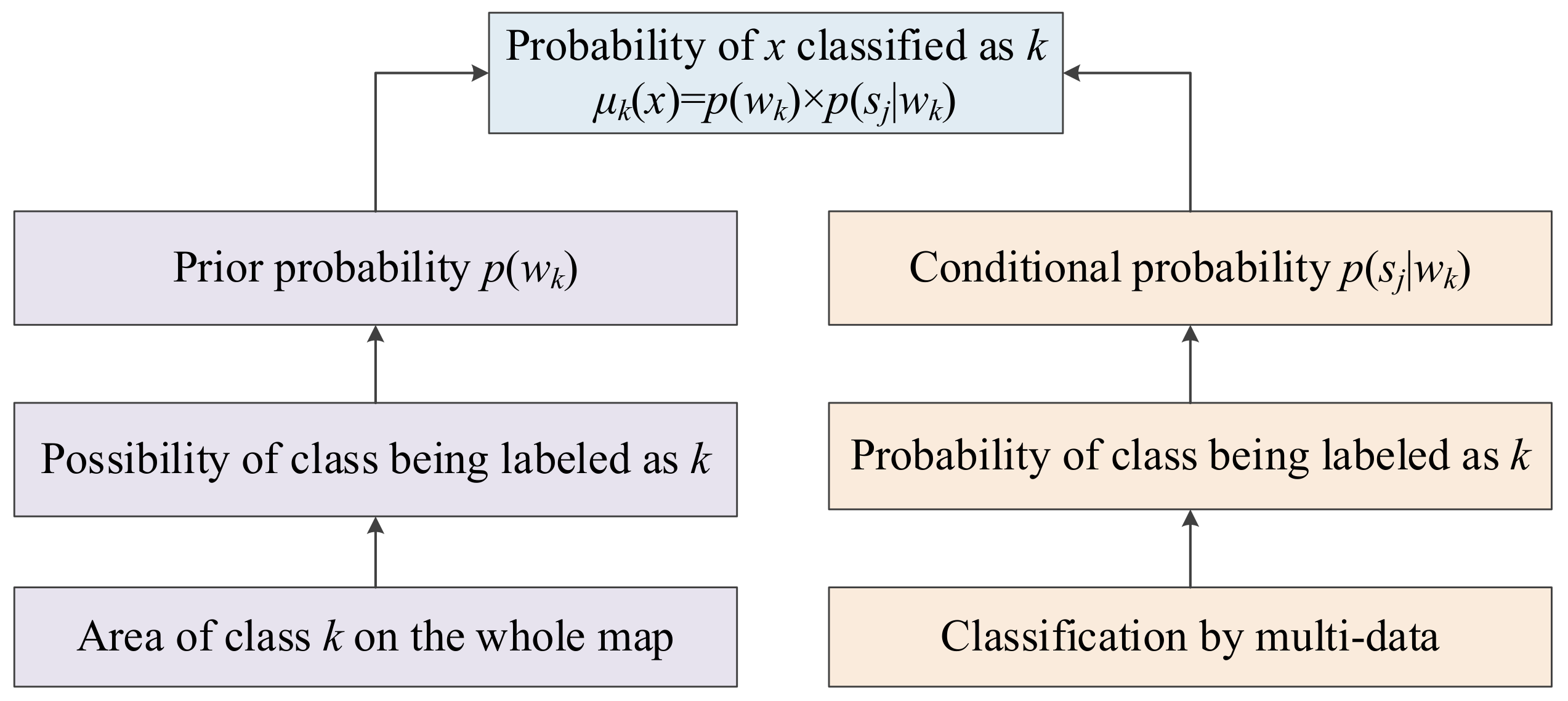
Figure 1. General workflow of the proposed method. The area of class k on the map denotes the possibility of k appearing on the whole map, thus used as prior probability in the Bayesian decision fusion formula. The multidata classification results are treated as the conditional probability of the x labeled as k after being carefully evaluated.
Remotesensing 14 06003 g001
Figure 2. Detailed flow chart of PBF. The process for acquiring the parameters is described.
Remotesensing 14 06003 g002
Figure 3. Image segmentation. The base image is an HSR remote sensing dataset (Landsat 8 OLI data): (a) is the segmentation of the Landsat image overlapped with a MODIS cell layer, and (b) is an example of segmentation results with a zoomed-in view constrained by four MODIS pixels. The four pixels from the HTR data appear as square black lines in green, red, yellow, and blue colors, respectively. The segmentation results also appear as black lines.
Remotesensing 14 06003 g003
Figure 4. Workflow of the comparison experiment in two cases.
Remotesensing 14 06003 g004
Figure 5. Location of the test site in Thailand.
Remotesensing 14 06003 g005
Figure 6. Distribution of samples. Group 1 is a union of groups 3, 4, and 5 and is shown in separate class symbols. Group 2 consists of selected pure-pixel points spread out over the map.
Remotesensing 14 06003 g006
Figure 7. The reference NDVI curves of MODIS selected by samples in AHB dataset.
Remotesensing 14 06003 g007
Figure 8. Memberships of grassland from (a) MODIS data; (b) Landsat data. The membership value is between 0 and 1.
Remotesensing 14 06003 g008
Figure 9. Single-source classification results of (a) MODIS and (b) Landsat data.
Remotesensing 14 06003 g009
Figure 10. Fusion result of the ESTARFM method with Landsat–MODIS pairs of date 4 January 2018 and 12 May 2018 as input and to predict on date 10 June 2017, 28 July 2017, 29 August 2017, 5 February 2018, 25 March 2018, 3 October 2018, 19 October 2018 and 6 December 2018.
Remotesensing 14 06003 g010
Figure 11. Classification result of the ESTARFM predicted time-series data in AHB dataset. (a) is the classification result of an objected-oriented method with the SVM classifier (i.e., LC4), and (b) is the classification result of the ED-similarity measure method (i.e., LC5).
Remotesensing 14 06003 g011
Figure 12. Fusion result of the PBF method in AHB dataset.
Remotesensing 14 06003 g012
Figure 13. Classification result of the ESTARFM in the Mun River Basin. (a) is the classification result of an objected-oriented method with the SVM classifier (i.e., LC4), and (b) is the classification result of the ED-similarity measure method (i.e., LC5).
Remotesensing 14 06003 g013
Figure 14. The inferred probability (posterior probability) for three classes of PBF in the Mun River Basin: (a) Paddy Rice, (b) Deciduous Forest, and (c) Evergreen Forest.
Remotesensing 14 06003 g014
Figure 15. Fusion results using the maximum-posterior possibility measure based on the PBF method in the Mun River Basin. (a) is the zoomed-in view of the PBF data, (b) is the zoomed-in view of the Landsat classification results, (c) is the zoomed-in view of the MODIS classification results, and (d) is the zoomed-in view of the manually interpreted map.
Remotesensing 14 06003 g015
Figure 16. Visualized confusion matrix of PBF result in the Mun River Basin.
Remotesensing 14 06003 g016
Figure 17. Fusion results using compromised decision fusion.
Remotesensing 14 06003 g017
Figure 18. Fusion results from using the product combination rule in PBF.
Remotesensing 14 06003 g018
Figure 19. Comparison of the estimated area for each land types derived from the samples, Landsat data, MODIS, and two PBF methods (respectively, with conjunction and product) in the Mun River Basin.
Remotesensing 14 06003 g019aRemotesensing 14 06003 g019b
Table 1. Area proportion of each class estimated by sample points.
Class (k) p w k   % Confidence Interval (95% Level)
Construction Land2.5[2.478, 2.522]
Crop119.6[18.962, 20.238]
Crop225.9[22.875, 28.925]
Gobi12.2[10.773, 13.627]
Grass land13.2[12.207, 14.193]
Slope field14.9[13.788, 16.012]
Wasteland10.1[9.160, 11.040]
Water1.6[1.435, 1.765]
Table 2. Class-wise classification accuracy obtained for Landsat and MODIS data.
Class-Wise Accuracy
(Landsat)
Class-Wise Accuracy
(MODIS)
Construction Land0.920.14
Crop10.750.77
Crop20.440.60
Gobi0.810.59
Grassland0.430.41
Slope filed0.620.13
Wasteland0.400.36
Water0.970.44
Table 3. Class and area group-wise classification accuracy for MODIS imagery.
CL 1C1 2C2 3GB 4GL 5SF 6WL 7WT 8
0–100.080.130.180.240.220.060.050.05
0–200.100.180.240.310.290.080.070.07
20–300.140.240.320.430.390.110.090.09
30–400.190.330.450.590.540.160.130.12
40–500.160.270.360.470.430.130.100.10
50–600.080.130.180.240.220.060.050.05
60–700.140.250.330.440.400.120.090.09
70–800.080.130.180.240.220.060.050.05
80–900.210.350.470.630.570.170.130.13
90–1000.220.380.510.670.620.180.140.14
1 GS—Construction Land. 2 C1—Crop1. 3 C2—Crop2. 4 GB—Gobi Land. 5 GL—Grassland. 6 SF—Slope field. 7 WL—Wasteland. 8 WT—Water.
Table 4. Comparison of the class-wise classification accuracy for each method in the AHB dataset.
LC1LC2LC3LC4LC5
Construction land0.920.140.960.950.23
Crop10.750.770.960.730.72
Crop20.440.600.640.530.61
Gobi0.810.590.860.820.62
Grassland0.430.410.430.400.41
Slope field0.620.130.570.620.43
Wasteland0.400.360.420.390.32
Water0.970.440.960.970.34
Overall accuracy0.6890.4250.7450.7190.537
Table 5. Class-wise and overall classification accuracy (%) obtained for MODIS, Landsat, PBF and two ESTARFM-based methods in the Mun River Basin.
AF 1DF 2DL 3EF 4GL 5OT 6PR 7AL 8WT 9WL 10OA
LC19.6022.6541.2055.903.256.2573.2120.7432.474.8452.56
LC28.0026.1930.8079.418.310.5373.228.7223.7611.1148.10
LC30.0022.7356.8441.185.880.0077.609.5228.5713.3357.23
LC411.3225.7339.3568.528.997.5374.2628.4630.6010.2254.23
LC57.5221.2631.6560.626.235.6973.6110.2630.338.2853.67
1 AF—Artificial Forest. 2 DF—Deciduous Forest. 3 DL—Dry Land. 4 EF—Evergreen Forest. 5 GL—Grass Land. 6 OT—Others. 7 PR—Paddy Rice. 8 AL—Urban and Construction Land (Artificial Land). 9 WT—Water. 10 WL—Wetland.
Table 6. Analysis of the misclassification of classification results.
Manually LabeledMODISLandsatPBF ResultMembership of Labeled Type
(Landsat)
Membership of Labeled Type
(MODIS)
AFOTDFOT00
DFWLDFGL0.9851740
DLDFEFEF0.9731320.023427
EFPRDFPR00.0867
GLOTPRAL00.180617
OTOTAFAL00.039621
PRPRPRWT0.9930070.997983
ALGLDFDF00.742504
WTPRWLWL00
WLPRDLPR0.9245680.569142
Table 7. Comparison of the class-wise and overall classification accuracy (%) for each dataset.
AFDFDLEFGLOTPRALWTWLOA
Landsat9.6022.6541.2055.903.256.2573.2120.7432.474.8452.56
MODIS8.0026.1930.8079.418.310.5373.228.7223.7611.1148.10
CBDF0.0018.0346.5742.053.670.0076.858.6726.099.2354.44
PBF0.0022.7356.8441.185.880.0077.609.5228.5713.3357.23
Table 8. Comparison of the class-wise and overall classification accuracy (%) for each dataset, including the PBF methods with product combination and conjunctive combination rules.
AFDFDLEFGLOTPRALWTWLOA
Landsat9.6022.6541.2055.903.256.2573.2120.7432.474.8452.56
MODIS8.0026.1930.8079.418.310.5373.228.7223.7611.1148.10
PBF (product)0.0020.0033.0365.229.520.0077.597.6933.330.0059.29
PBF (conjunction)0.0022.7356.8441.185.880.0077.609.5228.5713.3357.23
Publisher’s Note: MDPI stays neutral with regard to jurisdictional claims in published maps and institutional affiliations.