Comparative Analysis and Comprehensive Trade-Off of Four Spatiotemporal Fusion Models for NDVI Generation
Abstract
1. Introduction
- (1)
- Comprehensively evaluate the fusion results of each model in terms of spectral characteristics and spatial characteristics;
- (2)
- Analyze the application characteristics and accuracy of each model in different natural geographic areas;
- (3)
- Visually display the comprehensive trade-off results of two aspects and three indicators and provide suggestions for relevant scholars to choose the spatiotemporal fusion models for NDVI generation.
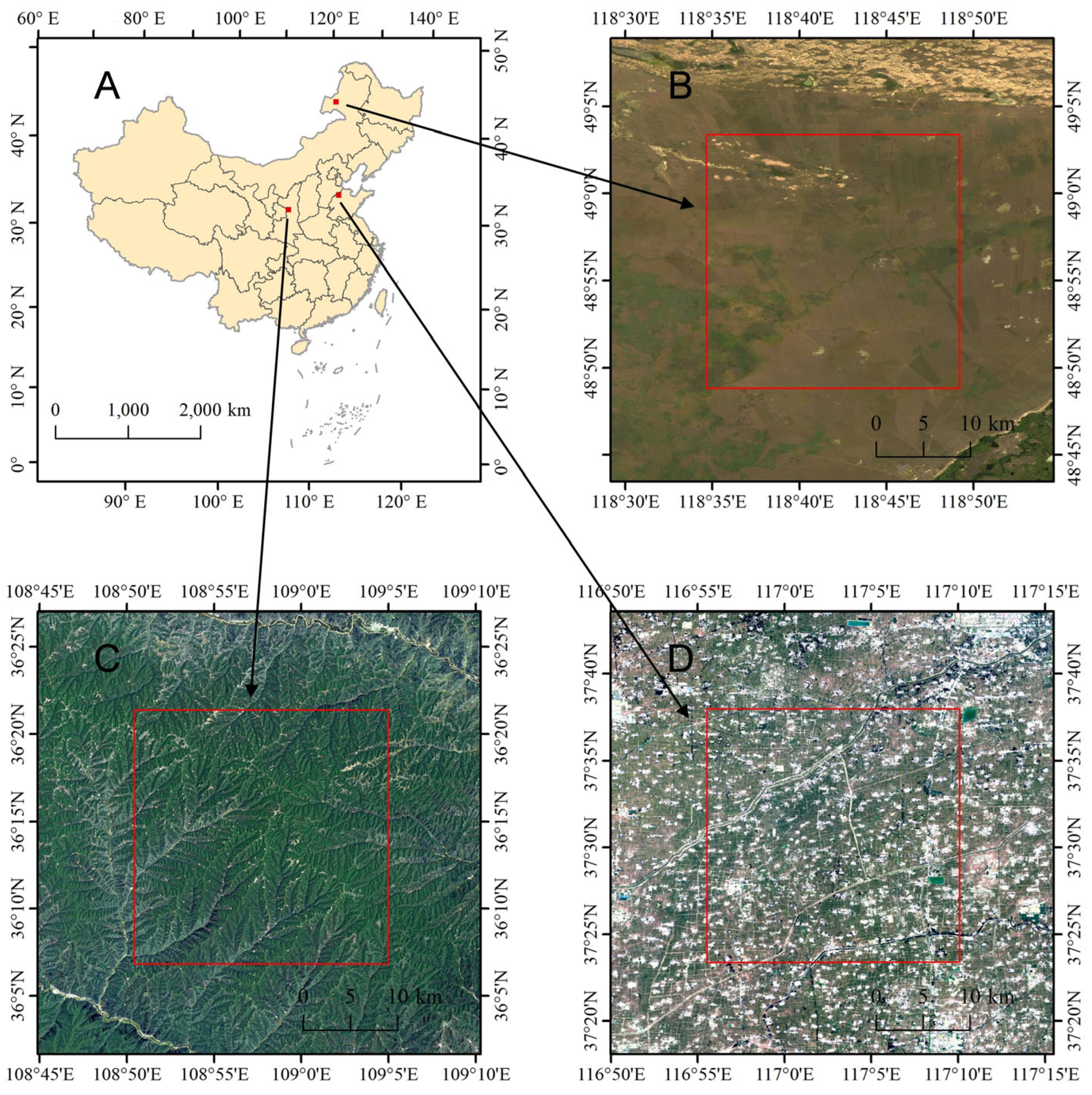
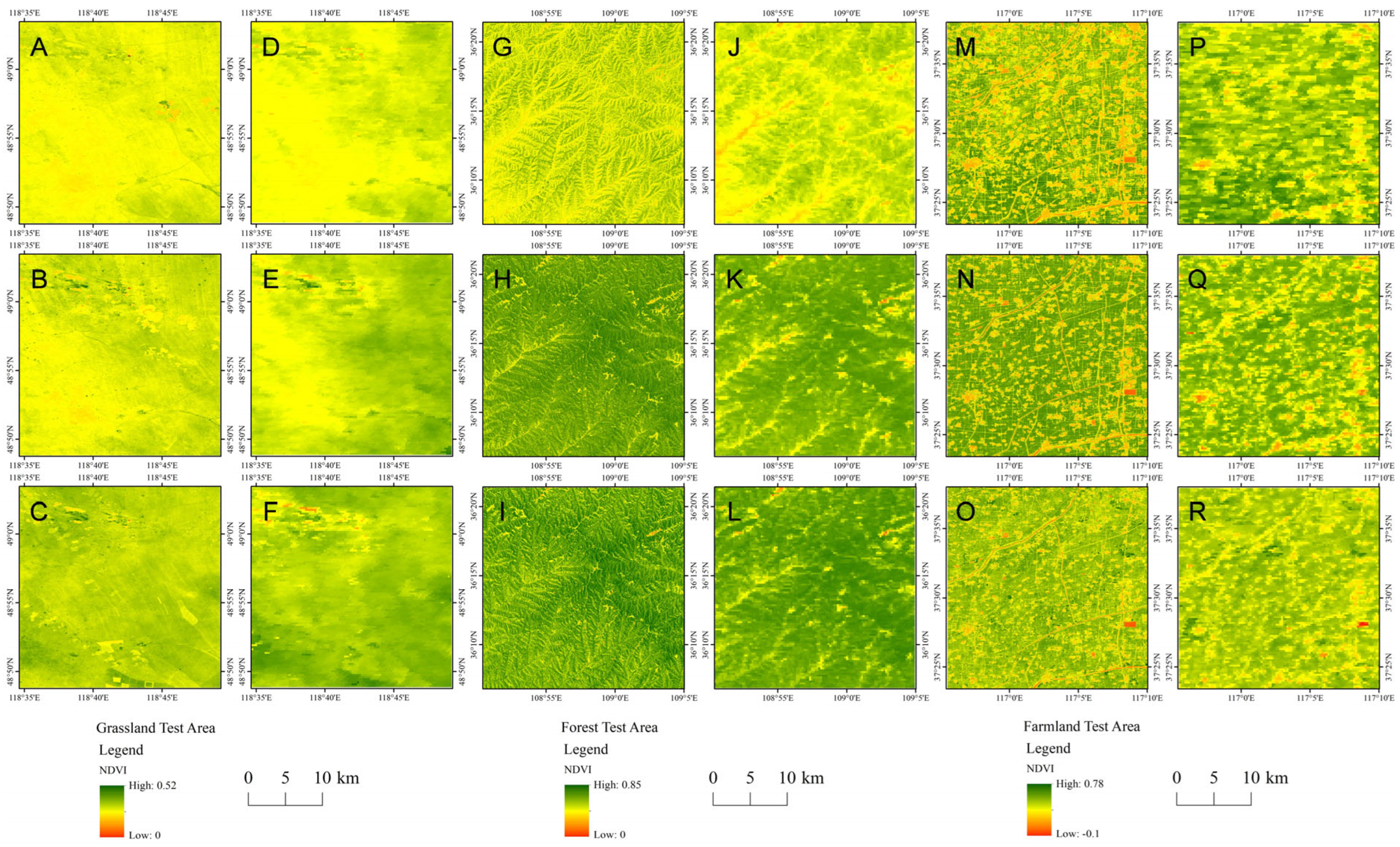
2. Test Areas and Data
3. Methods
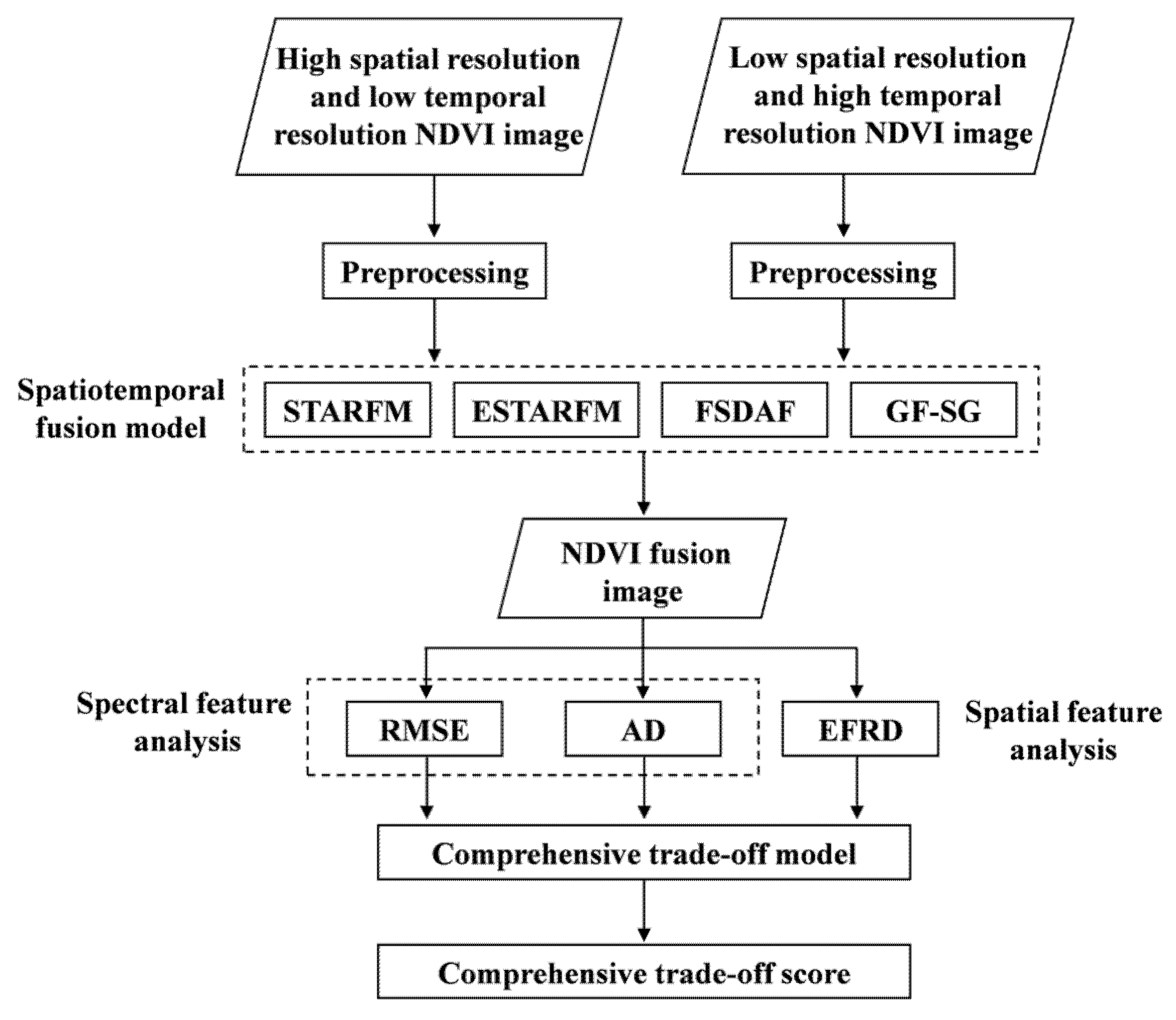
3.1. Overall Research Framework
3.2. Spatiotemporal Fusion Models
3.2.1. STARFM
- (1)
- Select candidates with similar image elements. In the fine-resolution image, each image element in turn is used as the central image element, and candidate similar image elements are selected for them using the neighborhood window and thresholding methods. The threshold is determined by the standard deviation of the fine-resolution image and the estimated number of land use/cover types.
- (2)
- Filtering samples. A constraint function is introduced to remove low-quality observations from the candidate similar elements.
- (3)
- Determine weights. A combination function is used to calculate the degree of influence of the similar image element on the central image element, i.e., the weight, considering three aspects: spectral difference, temporal difference, and distance difference.
- (4)
- Calculating central image element values. Using a weighting function, the fine-resolution image element values for the predicted period are calculated based on the spectral information of similar image elements combining fine-resolution and coarse-resolution data.
3.2.2. ESTARFM
- (1)
- Selection of similar image elements. ESTARFM uses the same threshold determination method as STARFM. However, since there are two pairs of fine-resolution and coarse-resolution NDVI data, ESTARFM first selects the candidate neighboring similar elements from the two pairs of images separately and then takes the intersection afterward.
- (2)
- Determination of weights. Considering the spectral difference and distance difference between the central image element and the similar image element, a combination function is used to calculate the weight of the similar image element.
- (3)
- Calculate the conversion factor. Based on the linear relationship between the spectral values of the image element and the end element in the coarse-resolution image, the end element is used as the fine-resolution image element in the coarse-resolution image element, and the slope is obtained by linear regression, which is called the conversion factor. The conversion factor characterizes the conversion relationship between coarse-resolution image elements (mixed image elements) and fine-resolution image elements.
- (4)
- Calculate the central image element value. Based on the similar image weights and conversion coefficients, the central image value is calculated for each input image pair separately to form the transition image. Then, based on the overall spectral similarity between their coarse-resolution image and the coarse-resolution image of the predicted date, the weights are determined, and the final central image element value is calculated.
3.2.3. FSDAF
- (1)
- Calculate richness. Based on the unsupervised classification method, the input fine-resolution images are classified, and the richness of the category is counted in each coarse-resolution image element.
- (2)
- Fitting the category change values. For each category, the coarse-resolution image elements with the highest richness are selected and their differences between the known and predicted periods are calculated; afterward, the change values of each fine-resolution image element are fitted by least squares.
- (3)
- Feature change correction. The coarse-resolution images of the predicted period are interpolated by three splines, the errors between homogeneous and heterogeneous areas are analyzed, and the two errors are combined by homogeneity coefficients to correct the change values.
- (4)
- Elimination of the “block effect”. Select adjacent similar image elements and calculate the weight value, then calculate the change value of the central image element based on the weight function. The change values are then superimposed on the fine-resolution image elements to obtain the result.
3.2.4. GF-SG
- (1)
- Pre-processing images. Select all the coarse resolution and fine resolution remote sensing images within a period (generally six months to one year), remove the parts of the images with clouds and cloud shadows, and calculate the NDVI.
- (2)
- Matching shapes. The coarse-resolution NDVI image is downscaled to fine resolution using double triple convolution, capturing the pattern of change and temporal shape of the coarse-resolution NDVI values on each fine image element. For each fine-resolution center image, the fine-resolution NDVI time shape is matched to the coarse-resolution image within a neighborhood window, and neighboring images with correlation coefficients greater than a threshold are identified as similar.
- (3)
- Fill time series. For each fine-resolution central image, the time shapes of the similar images are combined by weighting them as their reference time series, and the possible difference in magnitude between the fine-resolution and coarse-resolution image values is corrected by shape fitting. The corrected reference time series is used to fill in the missing values in the original fine-resolution NDVI image and to produce fine-resolution data between the two scenes of fine-resolution images.
- (4)
- Noise removal. The original fine-resolution NDVI values are given maximum weight, the image element values with a smaller standard deviation of adjacent pixels in the neighborhood are given larger weights, and the fine-resolution NDVI time series are smoothed using a weighted SG filter to remove the effects of residual cloud contamination as well as random noise and other factors.
3.3. Comparative Analysis Methods
3.3.1. Root Mean Square Error
3.3.2. Average Difference
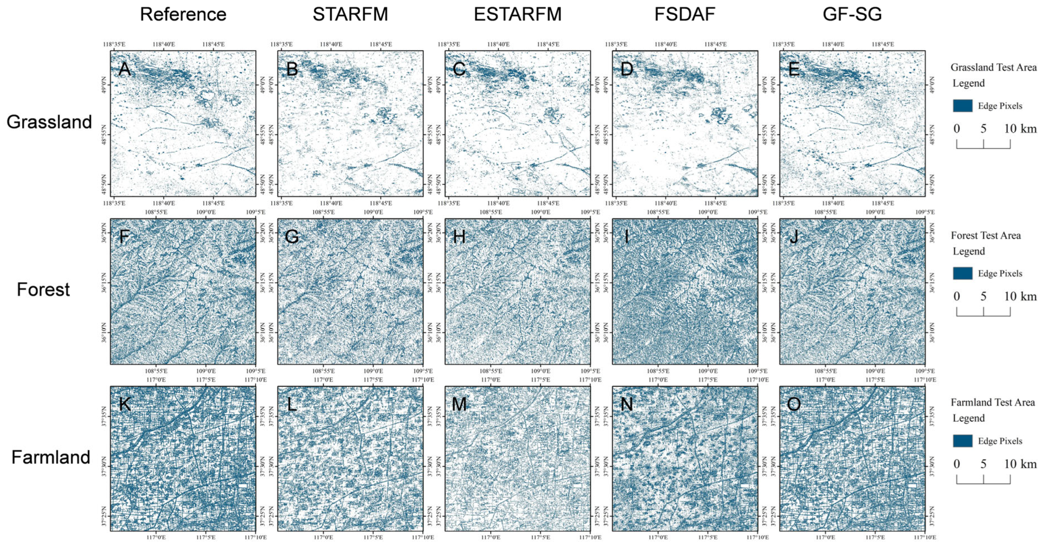
3.3.3. Edge Feature Richness Difference
3.3.4. Comprehensive Trade-Off Method
4. Results and Analysis
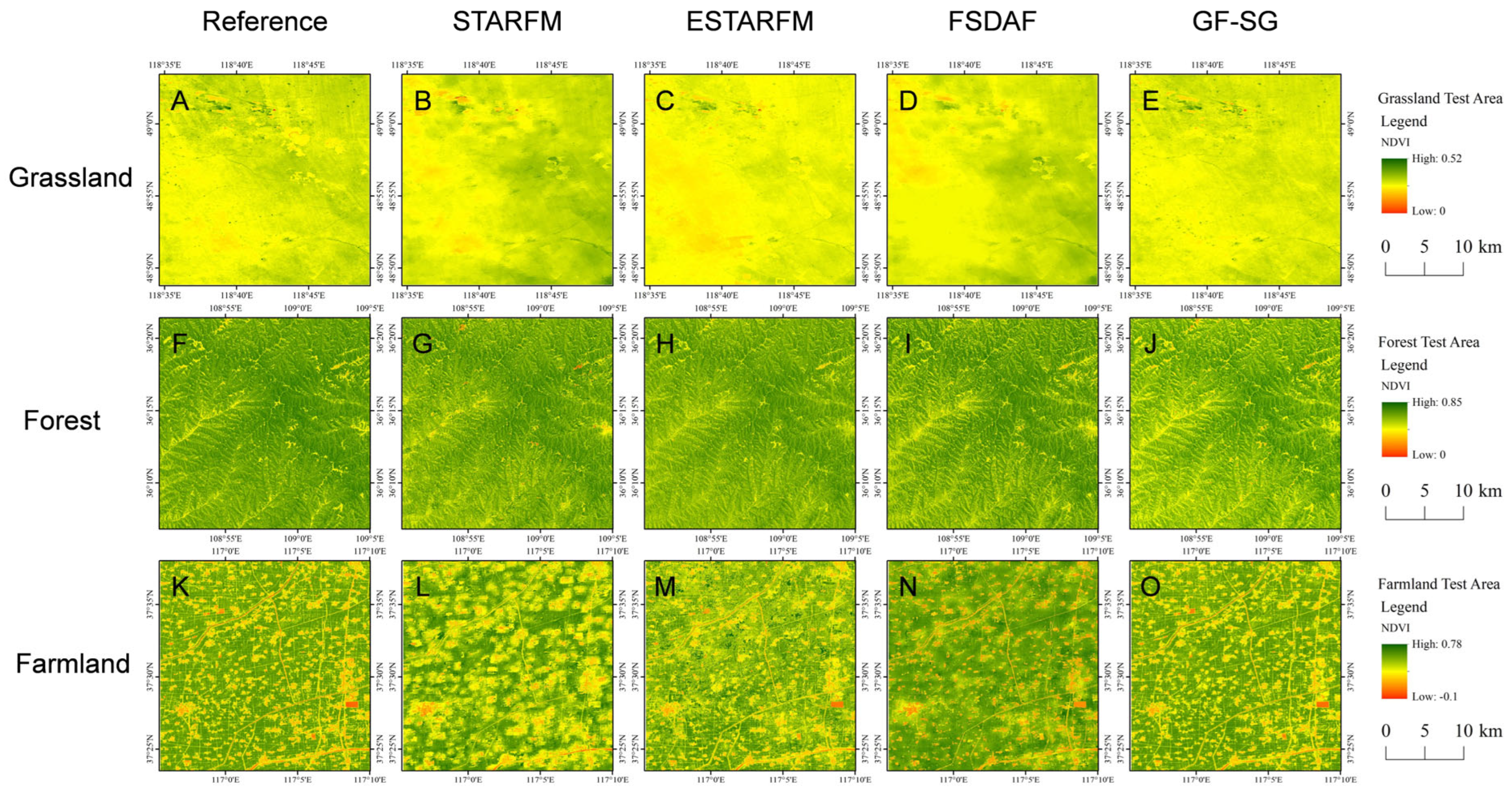
4.1. NDVI Fusion Results
4.2. Root Mean Square Error Analysis
4.3. Average Difference Analysis
4.4. Edge Feature Richness Difference Analysis
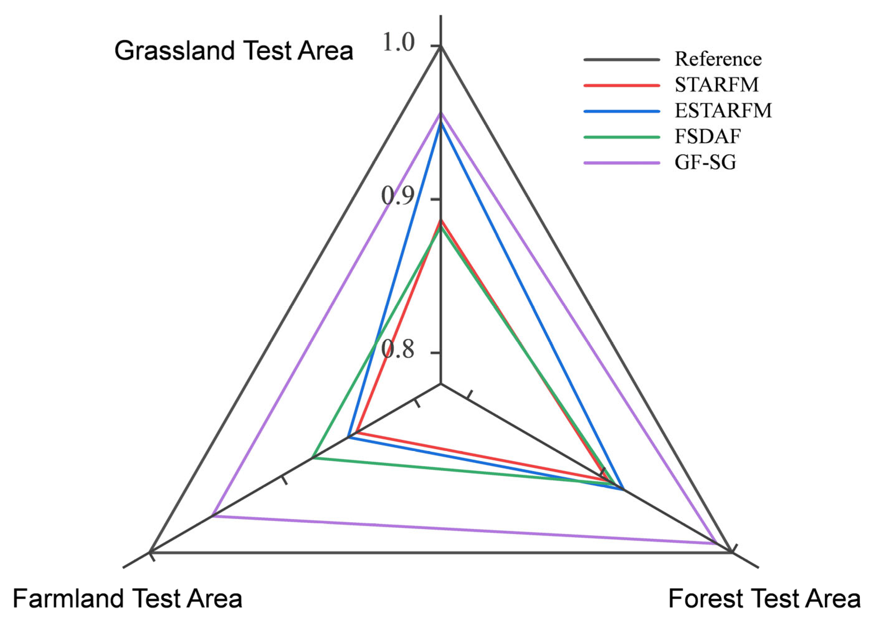
4.5. Comprehensive Trade-Off Analysis
5. Discussion
6. Conclusions
Author Contributions
Funding
Conflicts of Interest
References
- Zhang, W.; Randall, M.; Jensen, M.B.; Brandt, M.; Wang, Q.; Fensholt, R. Socio-economic and climatic changes lead to contrasting global urban vegetation trends. Glob. Environ. Chang. 2021, 71, 102385. [Google Scholar] [CrossRef]
- Cao, D.; Zhang, J.; Xun, L.; Yang, S.; Wang, J.; Yao, F. Spatiotemporal variations of global terrestrial vegetation climate potential productivity under climate change. Sci. Total Environ. 2021, 770, 145320. [Google Scholar] [CrossRef] [PubMed]
- Chen, J.; Fan, W.; Li, D.; Liu, X.; Song, M. Driving factors of global carbon footprint pressure: Based on vegetation carbon sequestration. Appl. Energy 2020, 267, 114914. [Google Scholar] [CrossRef]
- Wu, C.; Peng, D.; Soudani, K.; Siebicke, L.; Gough, C.M.; Arain, M.A.; Bohrer, G.; Lafleur, P.M.; Peichl, M.; Gonsamo, A.; et al. Land surface phenology derived from normalized difference vegetation index (NDVI) at global FLUXNET sites. Agric. For. Meteorol. 2017, 233, 171–182. [Google Scholar] [CrossRef]
- Prăvălie, R.; Sîrodoev, I.; Nita, I.-A.; Patriche, C.; Dumitraşcu, M.; Roşca, B.; Tişcovschi, A.; Bandoc, G.; Săvulescu, I.; Mănoiu, V.; et al. NDVI-based ecological dynamics of forest vegetation and its relationship to climate change in Romania during 1987–2018. Ecol. Indic. 2022, 136, 108629. [Google Scholar] [CrossRef]
- Fokeng, R.M.; Fogwe, Z.N. Landsat NDVI-based vegetation degradation dynamics and its response to rainfall variability and anthropogenic stressors in Southern Bui Plateau, Cameroon. Geosyst. Geoenviron. 2022, 1, 100075. [Google Scholar] [CrossRef]
- Lin, J.; Chen, W.; Qi, X.; Hou, H. Risk assessment and its influencing factors analysis of geological hazards in typical mountain environment. J. Clean. Prod. 2021, 309, 127077. [Google Scholar] [CrossRef]
- Li, C.; Li, H.; Li, J.; Lei, Y.; Li, C.; Manevski, K.; Shen, Y. Using NDVI percentiles to monitor real-time crop growth. Comput. Electron. Agric. 2019, 162, 357–363. [Google Scholar] [CrossRef]
- Li, S.; Xu, L.; Jing, Y.; Yin, H.; Li, X.; Guan, X. High-quality vegetation index product generation: A review of NDVI time series reconstruction techniques. Int. J. Appl. Earth Obs. Geoinf. 2021, 105, 102640. [Google Scholar] [CrossRef]
- Zhang, J. Multi-source remote sensing data fusion: Status and trends. Int. J. Image Data Fusion 2010, 1, 5–24. [Google Scholar] [CrossRef]
- Schmitt, M.; Zhu, X.X. Data fusion and remote sensing: An ever-growing relationship. IEEE Geosci. Remote Sens. Mag. 2016, 4, 6–23. [Google Scholar] [CrossRef]
- Hou, J.; Van Dijk, A.I.J.M.; Renzullo, L.J. Merging Landsat and airborne LiDAR observations for continuous monitoring of floodplain water extent, depth and volume. J. Hydrol. 2022, 609, 127684. [Google Scholar] [CrossRef]
- Wulder, M.A.; Roy, D.P.; Radeloff, V.C.; Loveland, T.R.; Anderson, M.C.; Johnson, D.M.; Healey, S.; Zhu, Z.; Scambos, T.A.; Pahlevan, N.; et al. Fifty years of Landsat science and impacts. Remote Sens. Environ. 2022, 280, 113195. [Google Scholar] [CrossRef]
- Sunny, D.S.; Islam, K.M.A.; Mullick, M.R.A.; Ellis, J.T. Performance study of imageries from MODIS, Landsat 8 and Sentinel-2 on measuring shoreline change at regional scale. Remote Sens. Appl. Soc. Environ. 2022, 28, 100816. [Google Scholar] [CrossRef]
- Skakun, S.; Wevers, J.; Brockmann, C.; Doxani, G.; Aleksandrov, M.; Batič, M.; Frantz, D.; Gascon, F.; Gómez-Chova, L.; Hagolle, O.; et al. Cloud Mask Intercomparison eXercise (CMIX): An evaluation of cloud masking algorithms for Landsat 8 and Sentinel-2. Remote Sens. Environ. 2022, 274, 112990. [Google Scholar] [CrossRef]
- Gao, F.; Hilker, T.; Zhu, X.L.; Anderson, M.C.; Masek, J.G.; Wang, P.J.; Yang, Y. Fusing Landsat and MODIS Data for Vegetation Monitoring. IEEE Geosci. Remote Sens. Mag. 2015, 3, 47–60. [Google Scholar] [CrossRef]
- Zhu, X.; Helmer, E.H.; Gwenzi, D.; Collin, M.; Fleming, S.; Tian, J.; Marcano-Vega, H.; Meléndez-Ackerman, E.J.; Zimmerman, J.K. Characterization of Dry-Season Phenology in Tropical Forests by Reconstructing Cloud-Free Landsat Time Series. Remote Sens. 2021, 13, 4736. [Google Scholar] [CrossRef]
- Ghassemian, H. A review of remote sensing image fusion methods. Inf. Fusion 2016, 32, 75–89. [Google Scholar] [CrossRef]
- Li, J.; Hong, D.; Gao, L.; Yao, J.; Zheng, K.; Zhang, B.; Chanussot, J. Deep learning in multimodal remote sensing data fusion: A comprehensive review. Int. J. Appl. Earth Obs. Geoinf. 2022, 112, 102926. [Google Scholar] [CrossRef]
- Gao, F.; Masek, J.; Schwaller, M.; Hall, F. On the blending of the Landsat and MODIS surface reflectance: Predicting daily Landsat surface reflectance. IEEE Trans. Geosci. Remote Sens. 2006, 44, 2207–2218. [Google Scholar] [CrossRef]
- Zhu, X.; Chen, J.; Gao, F.; Chen, X.; Masek, J.G. An enhanced spatial and temporal adaptive reflectance fusion model for complex heterogeneous regions. Remote Sens. Environ. 2010, 114, 2610–2623. [Google Scholar] [CrossRef]
- Liu, M.; Ke, Y.; Yin, Q.; Chen, X.; Im, J. Comparison of Five Spatio-Temporal Satellite Image Fusion Models over Landscapes with Various Spatial Heterogeneity and Temporal Variation. Remote Sens. 2019, 11, 2612. [Google Scholar] [CrossRef]
- Gevaert, C.M.; García-Haro, F.J. A comparison of STARFM and an unmixing-based algorithm for Landsat and MODIS data fusion. Remote Sens. Environ. 2015, 156, 34–44. [Google Scholar] [CrossRef]
- Chen, B.; Huang, B.; Xu, B. Comparison of Spatiotemporal Fusion Models: A Review. Remote Sens. 2015, 7, 1798–1835. [Google Scholar] [CrossRef]
- Huang, B.; Song, H. Spatiotemporal Reflectance Fusion via Sparse Representation. IEEE Trans. Geosci. Remote Sens. 2012, 50, 3707–3716. [Google Scholar] [CrossRef]
- Ping, B.; Meng, Y.S.; Su, F.Z. Comparisons of spatio-temporal fusion methods for GF-1 WFV and MODIS data. J. Geo-Inf. Sci. 2019, 21, 157–167. [Google Scholar]
- Wang, Q.; Atkinson, P.M. Spatio-temporal fusion for daily Sentinel-2 images. Remote Sens. Environ. 2018, 204, 31–42. [Google Scholar] [CrossRef]
- Zhu, X.; Helmer, E.H.; Gao, F.; Liu, D.; Chen, J.; Lefsky, M.A. A flexible spatiotemporal method for fusing satellite images with different resolutions. Remote Sens. Environ. 2016, 172, 165–177. [Google Scholar] [CrossRef]
- Wu, M.; Niu, Z.; Wang, C.; Wu, C.; Wang, L. Use of MODIS and Landsat time series data to generate high-resolution temporal synthetic Landsat data using a spatial and temporal reflectance fusion model. J. Appl. Remote Sens. 2012, 6, 063507. [Google Scholar]
- Zhu, X.; Zhan, W.; Zhou, J.; Chen, X.; Liang, Z.; Xu, S.; Chen, J. A novel framework to assess all-round performances of spatiotemporal fusion models. Remote Sens. Environ. 2022, 274, 113002. [Google Scholar] [CrossRef]
- Chen, Y.; Cao, R.; Chen, J.; Liu, L.; Matsushita, B. A practical approach to reconstruct high-quality Landsat NDVI time-series data by gap filling and the Savitzky–Golay filter. ISPRS-J. Photogramm. Remote Sens. 2021, 180, 174–190. [Google Scholar] [CrossRef]
- Guo, D.; Shi, W.; Hao, M.; Zhu, X. FSDAF 2.0: Improving the performance of retrieving land cover changes and preserving spatial details. Remote Sens. Environ. 2020, 248, 111973. [Google Scholar] [CrossRef]
- Cao, R.; Xu, Z.; Chen, Y.; Chen, J.; Shen, M. Reconstructing High-Spatiotemporal-Resolution (30 m and 8-Days) NDVI Time-Series Data for the Qinghai–Tibetan Plateau from 2000–2020. Remote Sens. 2022, 14, 3648. [Google Scholar]
- Maimaitijiang, M.; Sagan, V.; Sidike, P.; Hartling, S.; Esposito, F.; Fritschi, F.B. Soybean yield prediction from UAV using multimodal data fusion and deep learning. Remote Sens. Environ. 2020, 237, 111599. [Google Scholar] [CrossRef]
- Chen, X.Y.; Wang, S.A.; Zhang, B.Q.; Luo, L. Multi-feature fusion tree trunk detection and orchard mobile robot localization using camera/ultrasonic sensors. Comput. Electron. Agric. 2018, 147, 91–108. [Google Scholar] [CrossRef]
- Zhou, J.; Chen, J.; Chen, X.; Zhu, X.; Qiu, Y.; Song, H.; Rao, Y.; Zhang, C.; Cao, X.; Cui, X. Sensitivity of six typical spatiotemporal fusion methods to different influential factors: A comparative study for a normalized difference vegetation index time series reconstruction. Remote Sens. Environ. 2021, 252, 112130. [Google Scholar] [CrossRef]
- Zhou, X.J.; Wang, P.X.; Tansey, K.; Zhang, S.Y.; Li, H.M.; Wang, L. Developing a fused vegetation temperature condition index for drought monitoring at field scales using Sentinel-2 and MODIS imagery. Comput. Electron. Agric. 2020, 168, 105144. [Google Scholar] [CrossRef]
- Surya, S.R.; Simon, P. Automatic Cloud Removal from Multitemporal Satellite Images. J. Indian Soc. Remote Sens. 2015, 43, 57–68. [Google Scholar] [CrossRef]
- Nietupski, T.C.; Kennedy, R.E.; Temesgen, H.; Kerns, B.K. Spatiotemporal image fusion in Google Earth Engine for annual estimates of land surface phenology in a heterogenous landscape. Int. J. Appl. Earth Obs. Geoinf. 2021, 99, 102323. [Google Scholar] [CrossRef]
| Test Area | STARFM | ESTARFM | FSDAF | GF-SG |
|---|---|---|---|---|
| Grassland | 0.1118 | 0.0248 | 0.0668 | 0.0477 |
| Forest | 0.1359 | 0.0282 | 0.0413 | 0.0108 |
| Farmland | 0.1057 | 0.0738 | 0.1217 | 0.0166 |
| Test Area | STARFM | ESTARFM | FSDAF | GF-SG |
|---|---|---|---|---|
| Grassland | 0.0632 | −0.0203 | 0.062 | −0.0038 |
| Forest | −0.012 | −0.0193 | −0.0279 | −0.0003 |
| Farmland | 0.0606 | −0.0266 | 0.1002 | −0.031 |
| Test Area | STARFM | ESTARFM | FSDAF | GF-SG |
|---|---|---|---|---|
| Grassland | −16.22 | −10.17 | −21.53 | 7.72 |
| Forest | −12.78 | −18.81 | 18.8 | −2.4 |
| Farmland | −28.54 | −32.72 | −14.71 | −9.29 |
| Trade-Off Score | Comprehensive Trade-Off Score | |||
|---|---|---|---|---|
| Grassland | Forest | Farmland | ||
| STARFM | 0.8867 | 0.9064 | 0.8436 | 0.8789 |
| ESTARFM | 0.9503 | 0.9181 | 0.8465 | 0.9050 |
| FSDAF | 0.8823 | 0.9113 | 0.8768 | 0.8901 |
| GF-SG | 0.9566 | 0.9883 | 0.9526 | 0.9658 |
Publisher’s Note: MDPI stays neutral with regard to jurisdictional claims in published maps and institutional affiliations. |
© 2022 by the authors. Licensee MDPI, Basel, Switzerland. This article is an open access article distributed under the terms and conditions of the Creative Commons Attribution (CC BY) license (https://creativecommons.org/licenses/by/4.0/).
Share and Cite
Hu, Y.; Wang, H.; Niu, X.; Shao, W.; Yang, Y. Comparative Analysis and Comprehensive Trade-Off of Four Spatiotemporal Fusion Models for NDVI Generation. Remote Sens. 2022, 14, 5996. https://doi.org/10.3390/rs14235996
Hu Y, Wang H, Niu X, Shao W, Yang Y. Comparative Analysis and Comprehensive Trade-Off of Four Spatiotemporal Fusion Models for NDVI Generation. Remote Sensing. 2022; 14(23):5996. https://doi.org/10.3390/rs14235996
Chicago/Turabian StyleHu, Yunfeng, Hao Wang, Xiaoyu Niu, Wei Shao, and Yichen Yang. 2022. "Comparative Analysis and Comprehensive Trade-Off of Four Spatiotemporal Fusion Models for NDVI Generation" Remote Sensing 14, no. 23: 5996. https://doi.org/10.3390/rs14235996
APA StyleHu, Y., Wang, H., Niu, X., Shao, W., & Yang, Y. (2022). Comparative Analysis and Comprehensive Trade-Off of Four Spatiotemporal Fusion Models for NDVI Generation. Remote Sensing, 14(23), 5996. https://doi.org/10.3390/rs14235996


