Appendix B. Regularized Estimation Method
In this section, we describe a general regularized pseudo-likelihood parameter-estimation procedure for our proposed ST-LAR model in (
2), which applies to all the model specifications in this paper.
To ease notation, let
for short, let
denote the conditional probability of
being one given
, and let
denote the vector stacking the regressors
,
, and
in (
2) corresponding to
, for
and
. Let
denote the parameter vector at location
and time
t; using the notations given above, we can rewrite
in (
2) as
.
Let
denote the set of all parameters associated with the model (
2). In the absence of instantaneous spatial dependence, which leaves
conditionally independent given
, the (pseudo) log-likelihood, e.g., [
56] over
is given by the equally-weighted sum of the log conditional densities of
:
where
.
We assume that the location-specific
-coefficients and
-coefficients have a clustering pattern in space, and a fused LASSO-type penalty [
51] is imposed on the log-likelihood given by (
A1). Following the work by Li and Sang [
40], we first obtain a partial order of the observed spatial locations using a tree graph to facilitate computations while preserving spatial information. Then, homogeneity constraints are imposed on each pair of coefficients at two adjacent locations, where the adjacencies of locations are defined by the edges of the tree graph. We shall remark here that the graph used to construct the fused LASSO penalty can be different from the graph used to define the neighboring autoregressors in (
2).
Specifically, we first define location neighborhoods using a connected undirected graph
, with the
M spatial locations as its nodes. In practice, we can either use a Delaunay triangulation [
57] or a
k-nearest neighbors approach to construct such a graph
. Then, we assign the edges of
with Euclidean distances of the nodes as the edge weights. For edges with the same weights, we break the tie by adding a very small random perturbation to each edge weight. A compact representation of the neighboring structure of those spatial locations is given by a spanning tree of
, which is a connected subgraph of
with the same nodes but without any cycles. Then, the unique minimum spanning tree (MST) is obtained by minimizing the sum of edge weights among all the spanning trees of
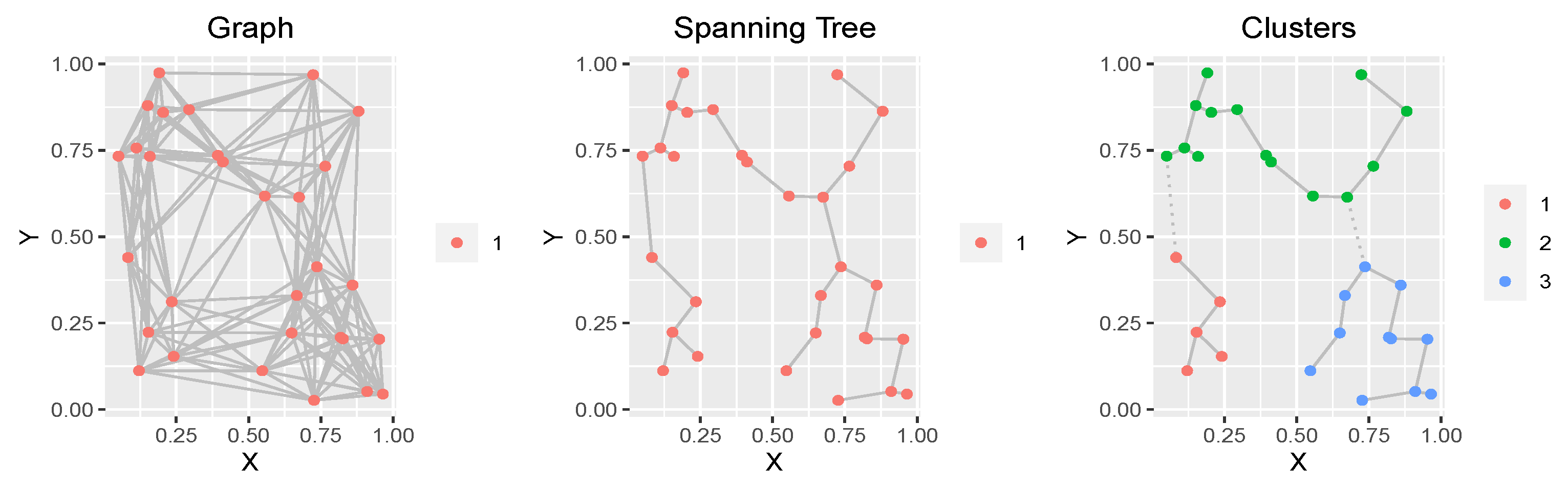
. For example, the left panel of
Figure A1 shows a connected graph
with 30 nodes, which is constructed by connecting each node with its 10 nearest-neighboring locations. The corresponding MST of
is shown in the middle panel of
Figure A1. Then, by deleting
edges from the MST, we can naturally define
r clusters as the
r sub-trees of the MST (see the right panel of
Figure A1 for the
clusters after removing the edges with the two largest weights).
Figure A1.
Left panel: A connected graph of 30 nodes, where each node is connected with its 10 nearest (according to Euclidean distance) neighbors, and edge weights are equal to the Euclidean distances between the nodes. Middle panel: The minimum spanning tree of . Right panel: The three induced clusters by removing two edges of the spanning tree (the two dotted lines).
Let
denote an MST of
, where
is the vertex set of
M nodes and
is the edge set. We minimize the following objective function:
where
denotes an edge in
connecting locations
and
, and
Thus, at each time
t, zero values of
,
, and
correspond to the edges connecting internal points of a cluster for the
-coefficients and the
-coefficients, respectively, while the nonzero values of these correspond to the edges connecting two boundary points across two clusters. For example, if
are only different at the adjacent locations connected by the dotted lines in the right panel of
Figure A1, we can obtain three clusters for the
k-th regression coefficient by deleting these two edges.
Suppose an edge connects two locations and for , where is the number of edges in the MST, and let denote the M-dimensional vector with only two nonzero entries: 1 at the i-th index and at the j-th. Then, , where , and and are similarly defined.
Let
denote the
contrast matrix; then, the penalized negative log-likelihood function can be written as
where
denotes the
norm of the vector
.
Following [
40], by letting
and
, we can re-parameterize the model parameters as
,
, and
, for
. Let
denote the vector of all the re-parameterized model parameters; since
is invertible by construction, minimizing the penalized negative log-likelihood in (
A3) is equivalent to minimizing
where
and
are the column vectors containing the first
entries of
and
, respectively. Minimizing the objective function in (
A4) is a standard LASSO problem whose computation is efficient. The best tuning parameter
in (
A4) is selected from a number of proposed values according to a model selection criterion, such as the Akaike information criterion (AIC, e.g., [
58]) or the Bayesian information criterion (BIC, e.g., [
59]). In our application to Arctic sea ice, we chose BIC to select
.
Appendix C. Detailed Model Comparison Results
To model the September Arctic sea ice data, consider the ST-LAR model in (
2) and its special cases as summarized in the following
Table A1. The Model-1 class only uses an intercept term
for modeling the mean of
, which has three sub-cases: (a) the intercept is constant and the
-coefficients are time-varying; (b) the intercept is time-varying and the
-coefficients vary in space and time; and (c) both the intercept term and the
-coefficients vary in space and time. Since for Model-1a the constant
is used instead of
, the design matrix of
,
, and
is of full rank. The Model-2 class incorporates June’s reflected solar radiation (RSR) as a covariate (denoted by
) in the ST-LAR model, which includes four sub-cases depending on whether the coefficients vary purely in time or vary in both space and time. The two classes and their sub-cases are specified in
Table A1.
Table A1.
The ST-LAR models for fitting the September Arctic SIE data. The mean of the latent is either modeled by an intercept term or by using the RSR as a covariate.
Table A1.
The ST-LAR models for fitting the September Arctic SIE data. The mean of the latent is either modeled by an intercept term or by using the RSR as a covariate.
| Model-1a | |
| Model-1b | |
| Model-1c | |
| Model-2a | |
| Model-2b | |
| Model-2c | |
| Model-2d | |
Model evaluation results of different ST-LAR models were obtained at
locations with at least one observed ice–water/water–ice transition in the last two decades. When implementing the regularized estimation given in
Appendix B, we tried different values of
ranging from
to 10 and selected the best one using the BIC criterion. The selected
values are different at different years, and the median value is about
.
Initialization for Estimation. Our proposed ST-LAR model given by (
2) requires (centered) past observations at time
as autoregressors to model the ice probability at time
t. At the initial year
, since the means of
(i.e.,
) are not available, we set
-coefficients in model (
2) to zero and only use
-coefficients to fit the binary observations at
. After we obtain the estimates
, we can fully employ the ST-LAR models in
Table A1 and obtain the estimated ice probabilities in a progressive manner from
onwards.
Results of the Model-1 Class. We first considered Model-1a, which uses a constant intercept for modeling the mean of and assumes only time-varying -coefficients. We used all the data to estimate the intercept through a classical logistic regression, assuming no space-time dependence among the observations. Then, by fixing at its estimate, a simple logistic regression was used to estimate and at each time point.
The corresponding model fitting results of Model-1a are given in the left columns of
Table A2. We observe that the MSE values are generally large compared to those in the middle and right columns, and the correct classification rates using the
cut-off value are generally below
. This indicates that only using the constant
-coefficients at each time point is not flexible enough to capture the spatial behaviors of ice–water/water–ice transitions. Then, we considered a more flexible model allowing the
-parameters to vary in space and time (Model-1b), and it can be seen that the fitting results are greatly improved (see the middle columns of
Table A2): The averaged MSE has reduced from Model-1a by a factor between 3 and 4, and the averaged correct classification rate is about
compared to
for Model-1a, indicating that the fitted ice probabilities can capture the observations very well. When further allowing the intercept to vary in space and time (Model-1c), the resulting averaged model evaluation scores are only slightly better than those of Model-1b. We observe that improvements in prediction accuracy for Model-1c occur for years 2004, 2008, 2013, 2016, 2017, and 2020. The performances of Model-1b and Model-1c are generally comparable, but Model-1b yields relatively lower correct classification rates at
(
) and
(
).
Table A2.
Model evaluation scores: The mean squared errors (MSEs), Nash–Sutcliffe model efficiency coefficients (NSEs), and the correct classification rates (CRs) for the Model-1 class based on their estimates at . The last row gives the time-averaged model evaluation scores.
Table A2.
Model evaluation scores: The mean squared errors (MSEs), Nash–Sutcliffe model efficiency coefficients (NSEs), and the correct classification rates (CRs) for the Model-1 class based on their estimates at . The last row gives the time-averaged model evaluation scores.
| | Model-1a | Model-1b | Model-1c |
|---|
| Year | MSE | NSE | CR | MSE | NSE | CR | MSE | NSE | CR |
| 2001 | | | | | | | | | |
| 2002 | | | | | | | | | |
| 2003 | | | | | | | | | |
| 2004 | | | | | | | | | |
| 2005 | | | | | | | | | |
| 2006 | | | | | | | | | |
| 2007 | | | | | | | | | |
| 2008 | | | | | | | | | |
| 2009 | | | | | | | | | |
| 2010 | | | | | | | | | |
| 2011 | | | | | | | | | |
| 2012 | | | | | | | | | |
| 2013 | | | | | | | | | |
| 2014 | | | | | | | | | |
| 2015 | | | | | | | | | |
| 2016 | | | | | | | | | |
| 2017 | | | | | | | | | |
| 2018 | | | | | | | | | |
| 2019 | | | | | | | | | |
| 2020 | | | | | | | | | |
| Average | | | | | | | | | |
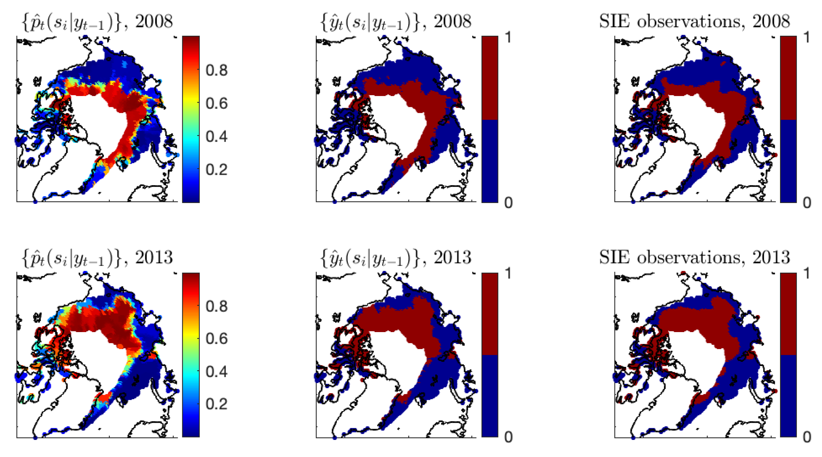
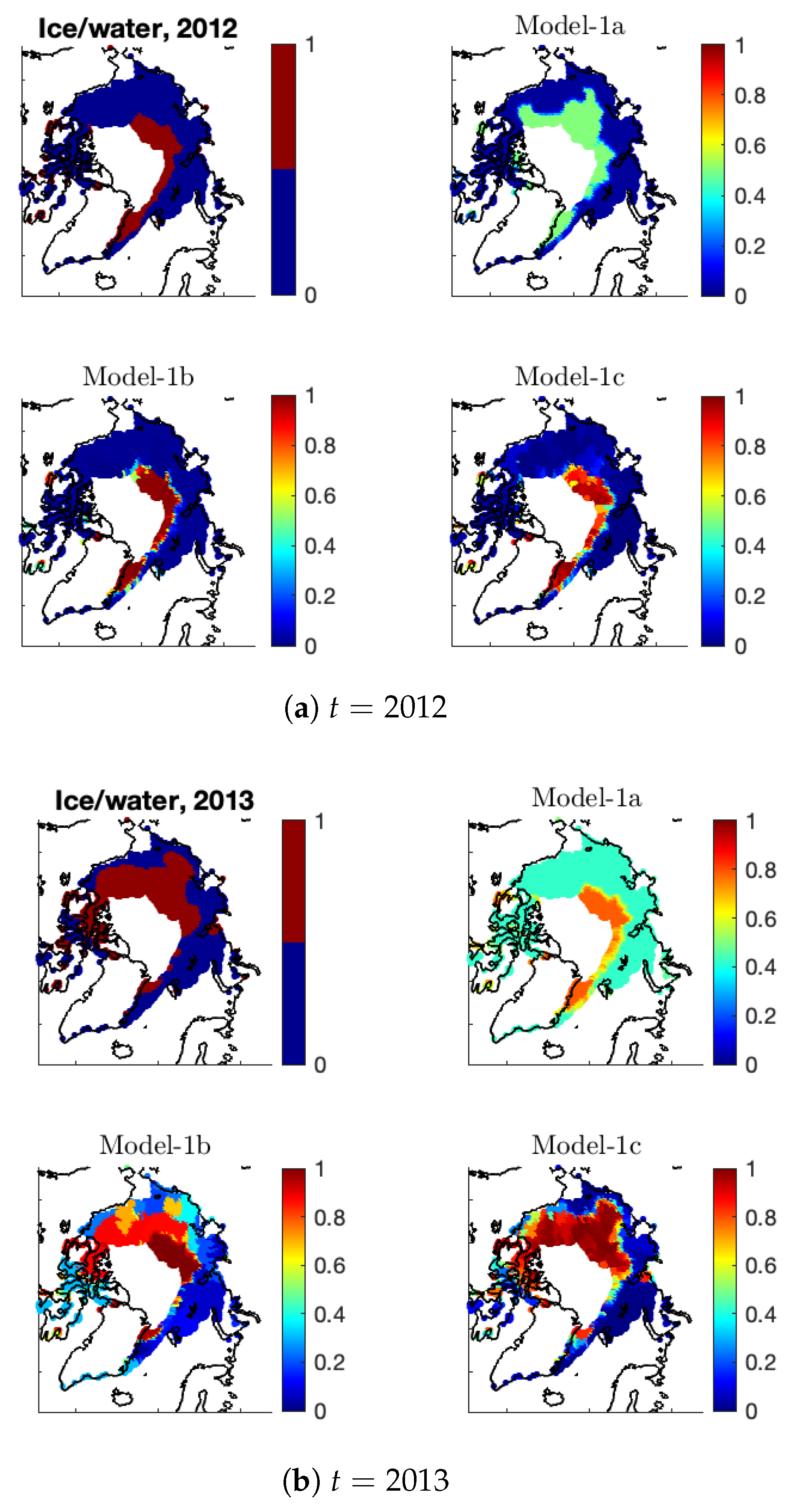
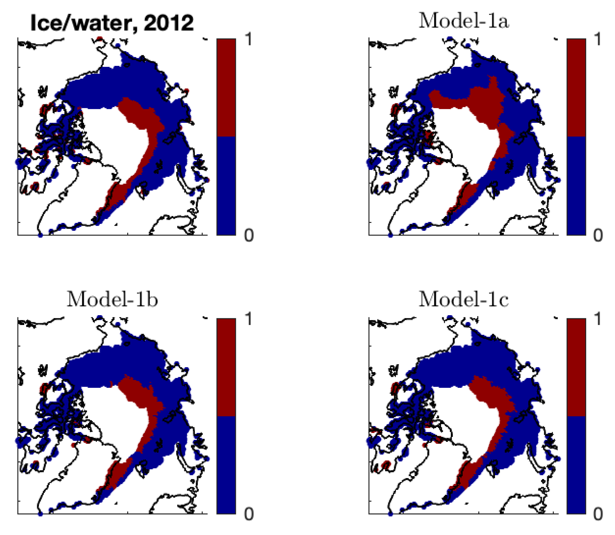
Figure A2 shows the estimates of
made by different models versus the observed SIE data at years
. It is clear that the simple autoregressive model with parameters
cannot capture the spatial patterns of the ice/water statuses at time
t; in fact, its estimated probabilities behave similarly to the immediate past observations at
. In contrast, by allowing the
-coefficients to vary in space and time, Model-1b can capture the main spatial patterns of the observed ice/water statuses, resulting in the estimates of
behaving very similarly to the observations. We can see that in 2012, the estimates of
by Model-1b are almost dichotomized, with small variations in the ice–water boundary regions. In the following year, 2013, Model-1b does not have the flexibility to capture the dramatic ice–water transitions, resulting in an estimated probability surface of substantial variability. Here, the fitted probabilities of Model-1c, which further allows the intercept to vary in space as well as time, behave more similarly to the observations.
Figure A2.
For each of (a) and (b) , shown are the observed ice/water statuses (upper-left panel) and the estimated ice probabilities by Model-1a (upper-right panel), Model-1b (lower-left panel), and Model-1c (lower-right panel).
Figure A2.
For each of (a) and (b) , shown are the observed ice/water statuses (upper-left panel) and the estimated ice probabilities by Model-1a (upper-right panel), Model-1b (lower-left panel), and Model-1c (lower-right panel).
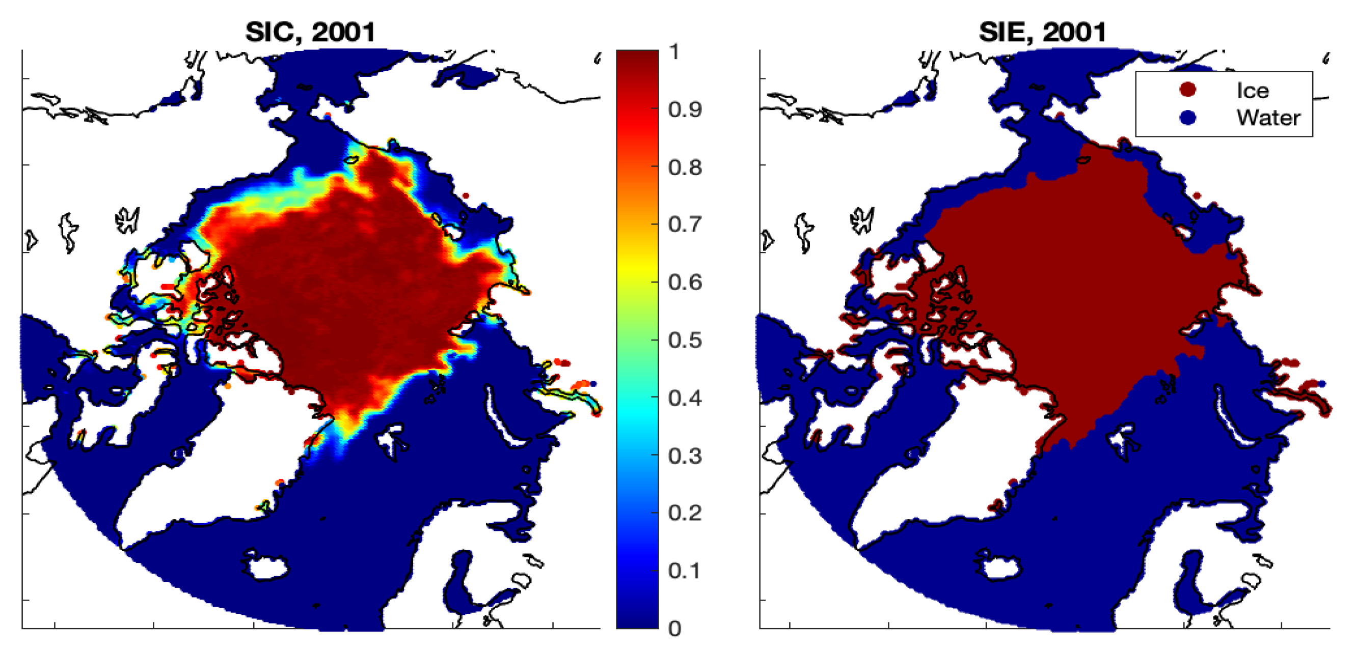
In addition, we obtain the binary estimates
by applying the cut-off value of
to dichotomize the sea-ice concentration estimates
. Both Model-1b and Model-1c lead to estimated ice/water statuses that are very similar to the observed statuses (see
Figure A3).
Figure A3.
The observed ice/water status and the estimated ice/water status (by Model-1a, Model-1b, and Model-1c) at .
Figure A3.
The observed ice/water status and the estimated ice/water status (by Model-1a, Model-1b, and Model-1c) at .
Results of the Model-2 Class. Zhan and Davies [
20] used the June RSR data to estimate the September Arctic sea ice with good success. This motivates us to include the June RSR as a covariate in our new model given by (
2) to see whether the model evaluation scores can be improved further. At each time
t, we standardized the RSR data by subtracting the sample means over space and dividing by the corresponding standard deviations. The CERES EBAF data product is on a
longitude–latitude grid, whose resolution is different from the 25 km resolution of the remotely sensed Arctic sea-ice data. When modeling
, we used the June RSR value at the location nearest to
as its RSR covariate.
The results of the Model-2 class are given in
Table A3, where the clear-sky RSR (CS-RSR) was used as a covariate when modeling
. For the model (
2) with spatially constant coefficients
, after incorporating the CS-RSR as a covariate (Model-2a), the correct classification rates have improved somewhat, with an averaged correct classification rate of
, compared to
with Model-1a. Especially for year
, from
Table A2, Model-1a has a very low correct classification rate of
and a very small NSE value of
. By borrowing information from the CS-RSR in 2013,
Table A3 shows that Model-2a achieves an improved correct classification rate of
and a much bigger NSE score. Changing the CS-RSR covariate to the AS-RSR covariate made very little difference in terms of the three model evaluation scores.
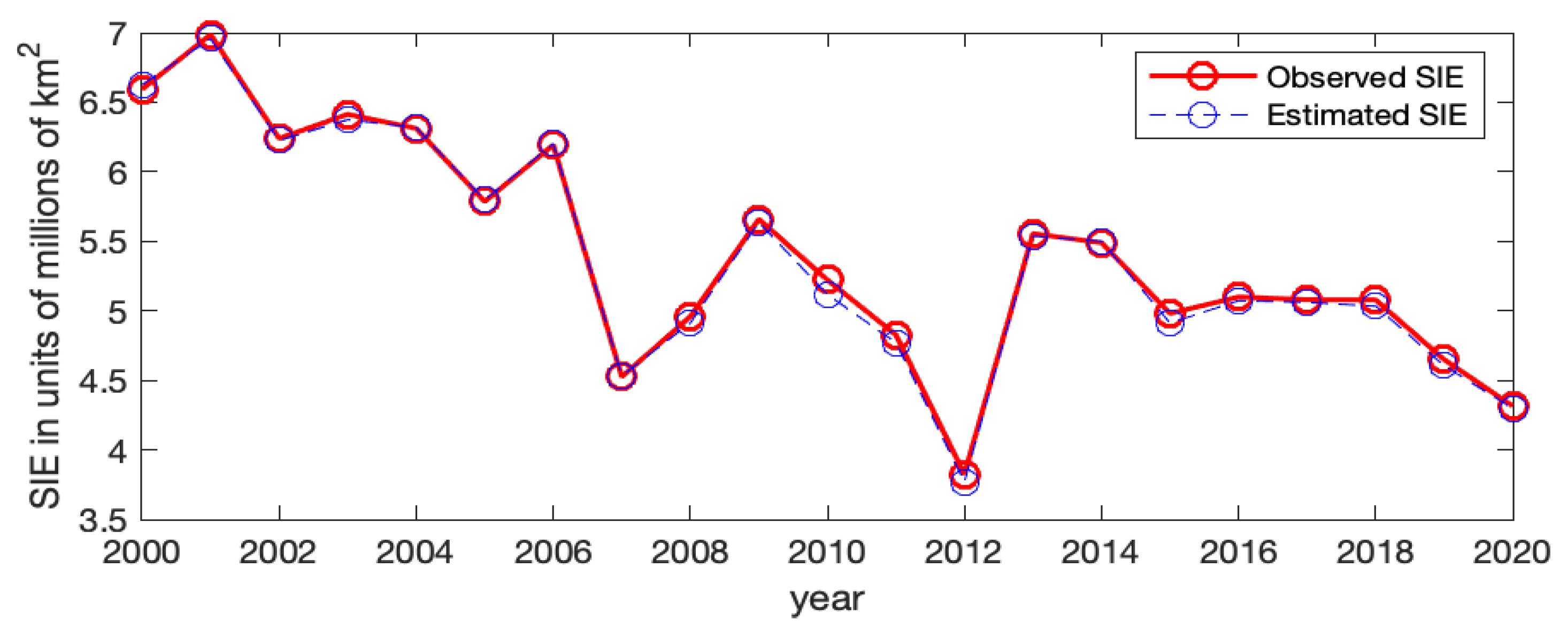
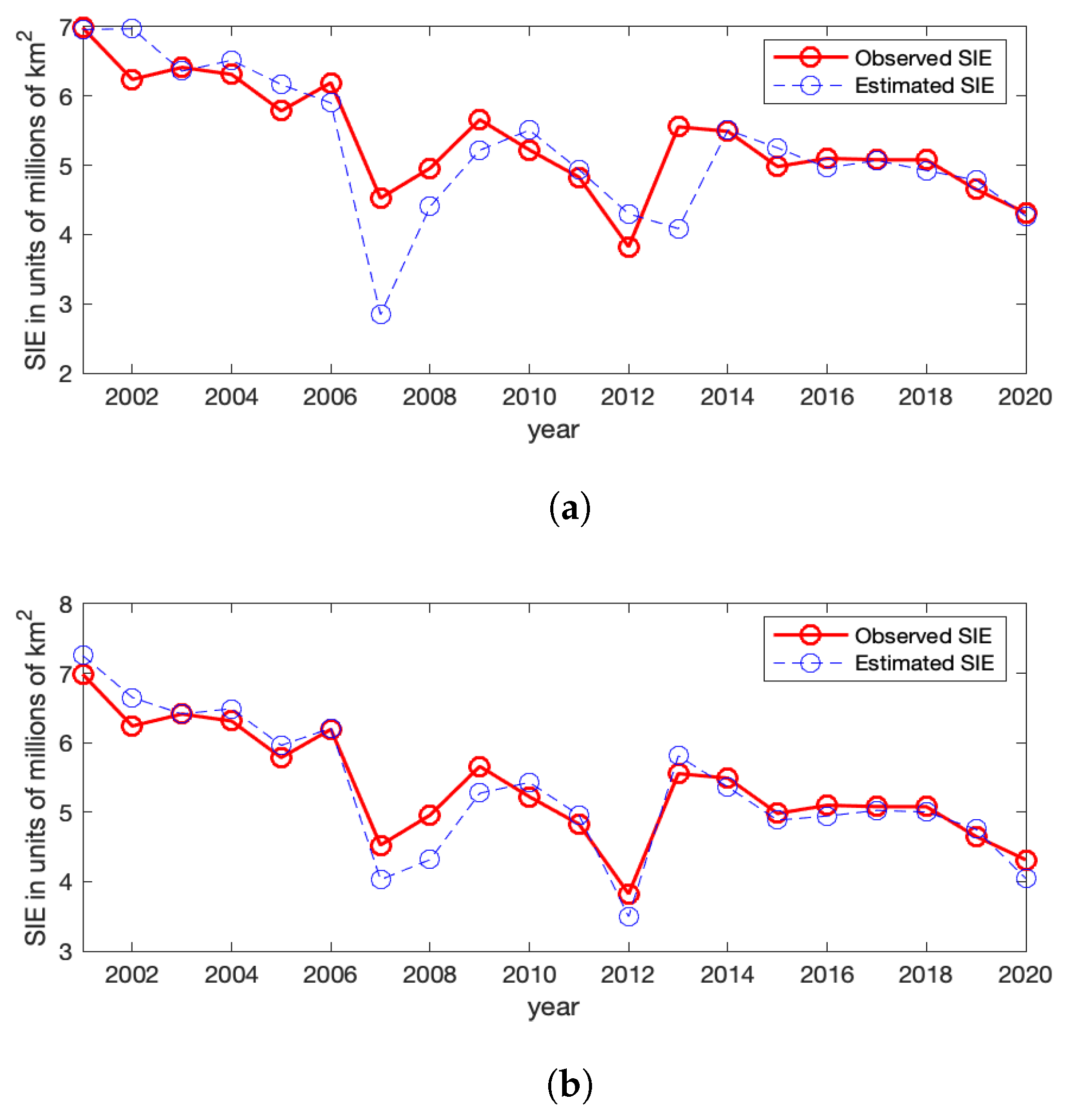
Figure A4 shows the observed Arctic SIE values and the estimated ones for Model-1a and Model-2a without and with CS-RSR, respectively. For Model-1a, which does not involve the RSR covariate, its ice/water statuses have large discrepancies with the observed values at a few years, and the general temporal trend of the SIEs cannot be captured; for example, the fitted Arctic SIEs are much smaller than the observed values at
and 2013. In contrast, when incorporating the June RSR information into the model (Model-2a), the estimated ice/water statuses are much closer to the observed values. Hence, the June RSR variable seems to be helpful for modeling Arctic sea ice.
Table A3.
The MSEs, NSEs, and CRs for the Model-2 class with clear-sky RSR (CS-RSR) as a covariate. The last row gives the time-averaged model evaluation scores.
Table A3.
The MSEs, NSEs, and CRs for the Model-2 class with clear-sky RSR (CS-RSR) as a covariate. The last row gives the time-averaged model evaluation scores.
| | Model-2a | Model-2b | Model-2c | Model-2d |
|---|
| Year | MSE | NSE | CR | MSE | NSE | CR | MSE | NSE | CR | MSE | NSE | CR |
| 2001 | | | | | | | | | | | | |
| 2002 | | | | | | | | | | | | |
| 2003 | | | | | | | | | | | | |
| 2004 | | | | | | | | | | | | |
| 2005 | | | | | | | | | | | | |
| 2006 | | | | | | | | | | | | |
| 2007 | | | | | | | | | | | | |
| 2008 | | | | | | | | | | | | |
| 2009 | | | | | | | | | | | | |
| 2010 | | | | | | | | | | | | |
| 2011 | | | | | | | | | | | | |
| 2012 | | | | | | | | | | | | |
| 2013 | | | | | | | | | | | | |
| 2014 | | | | | | | | | | | | |
| 2015 | | | | | | | | | | | | |
| 2016 | | | | | | | | | | | | |
| 2017 | | | | | | | | | | | | |
| 2018 | | | | | | | | | | | | |
| 2019 | | | | | | | | | | | | |
| 2020 | | | | | | | | | | | | |
| Overall | | | | | | | | | | | | |
Figure A4.
The observed Arctic SIE versus the estimated Arctic SIE using Model-1a and Model-2a (with the CS-RSR covariate). (a) Observed (red solid line) and estimated (blue dashed line) Arctic SIE using Model-1a with coefficients . (b) Observed (red solid line) and estimated (blue dashed line) Arctic SIE using Model-2a with the CS-RSR covariate.
However, when further allowing the
-coefficients to vary in both space and time, incorporating the RSR covariate (Model-2b) does not improve the model evaluation scores on average, and the resulting averaged scores are comparable to those with Model-1b (and Model-1c). Similar conclusions hold for the even-more-flexible models Model-2c and Model-2d with regression coefficients varying in space and time. It seems that the spatially varying
-coefficients are already flexible enough to capture the spatial patterns of
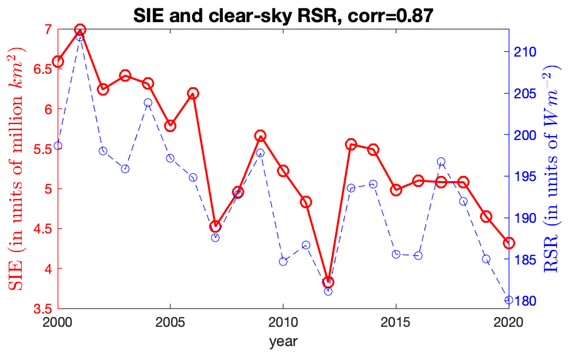
. Although the spatially averaged RSR values are highly correlated with the Arctic SIEs as shown in
Figure 5, the local spatial patterns of the June RSR do not match very well with those of sea ice.
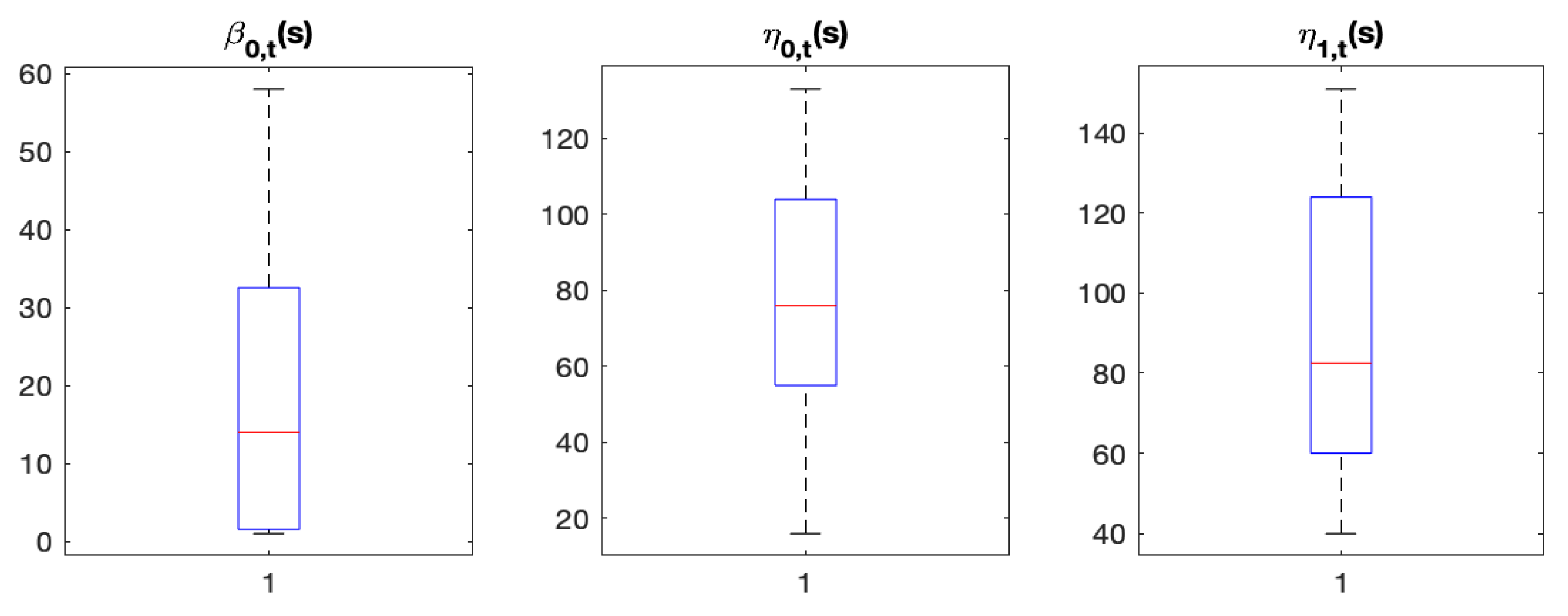
More Validation Results for Model-1c. We first check the number of distinct model parameters for Model-1c.
Figure A5 shows the boxplots of the numbers of distinct values for the
and
-coefficients. We can see that the numbers of distinct coefficients are small relative to the sample size (which is
), with median values less than 100. The largest number of model parameters of the fitted ST-LAR models is about 300, which is much smaller than the sample size. Therefore, the model we choose (Model-1c) does not obviously suffer from over-fitting.
Figure A5.
Boxplots of the numbers of distinct coefficients at years 2001–2020 for Model-1c.
Figure A5.
Boxplots of the numbers of distinct coefficients at years 2001–2020 for Model-1c.
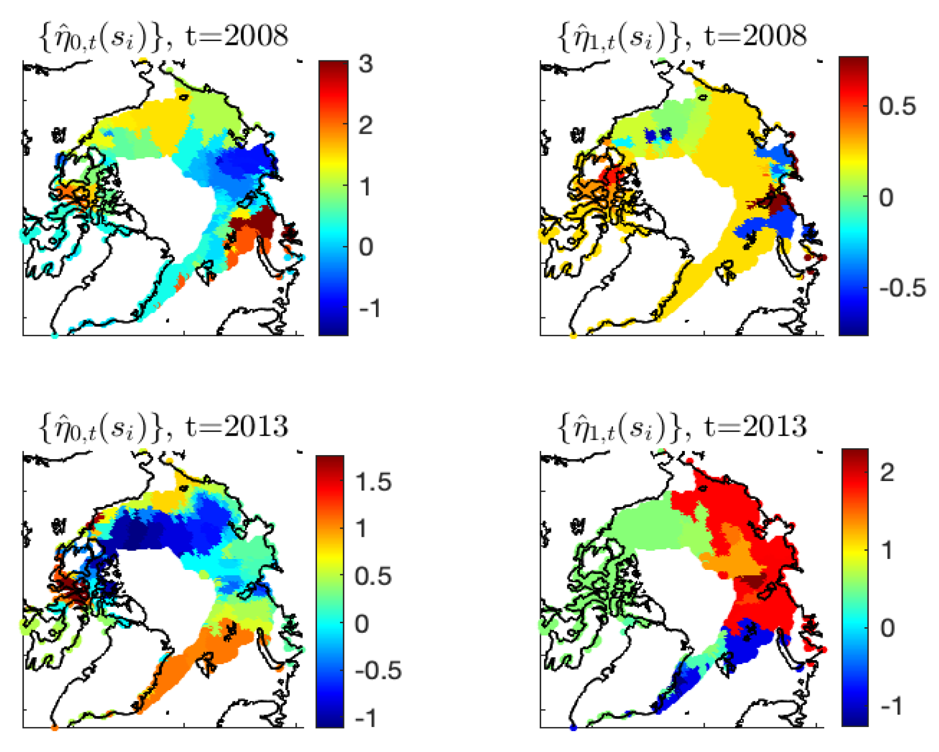
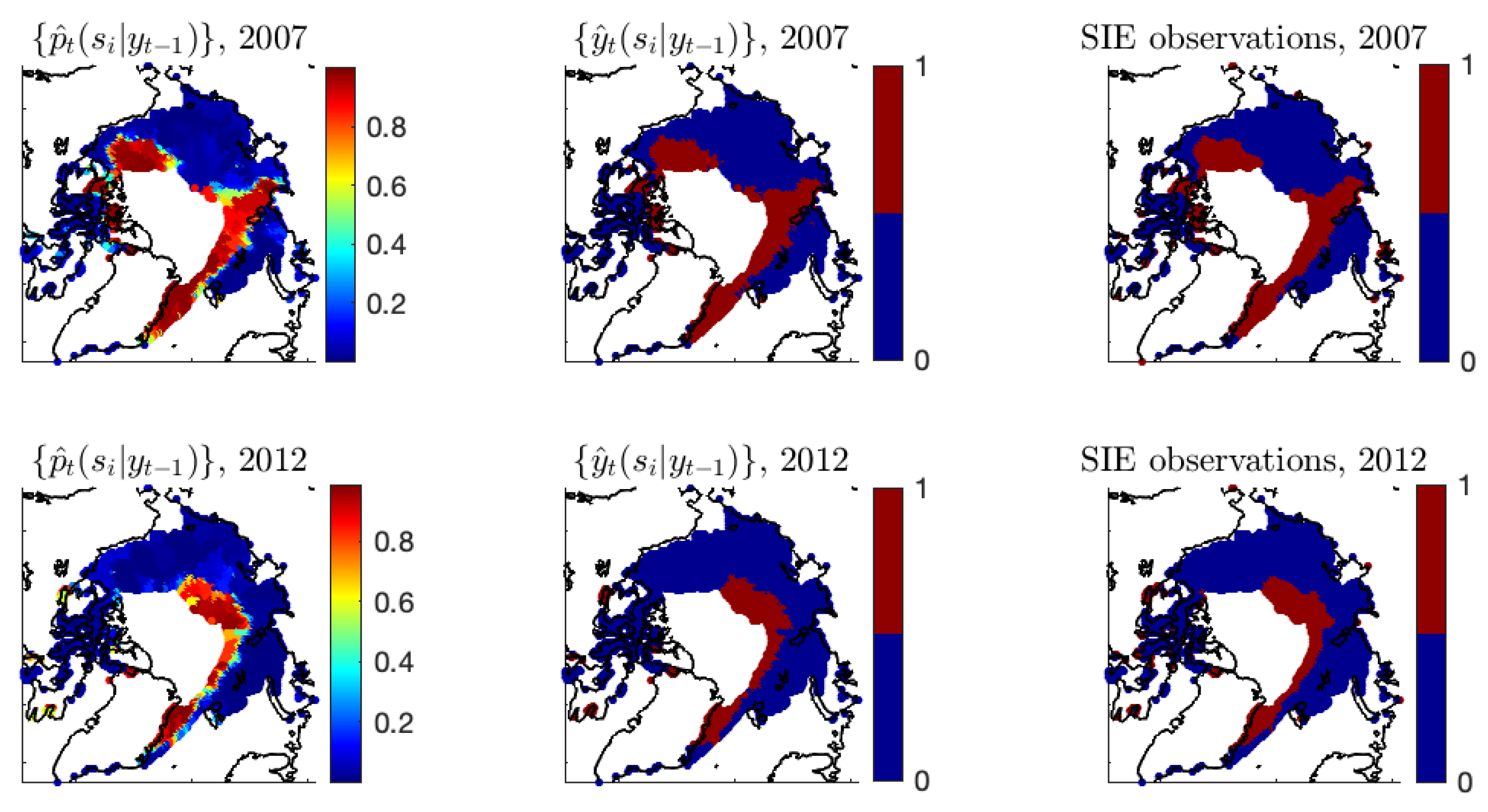
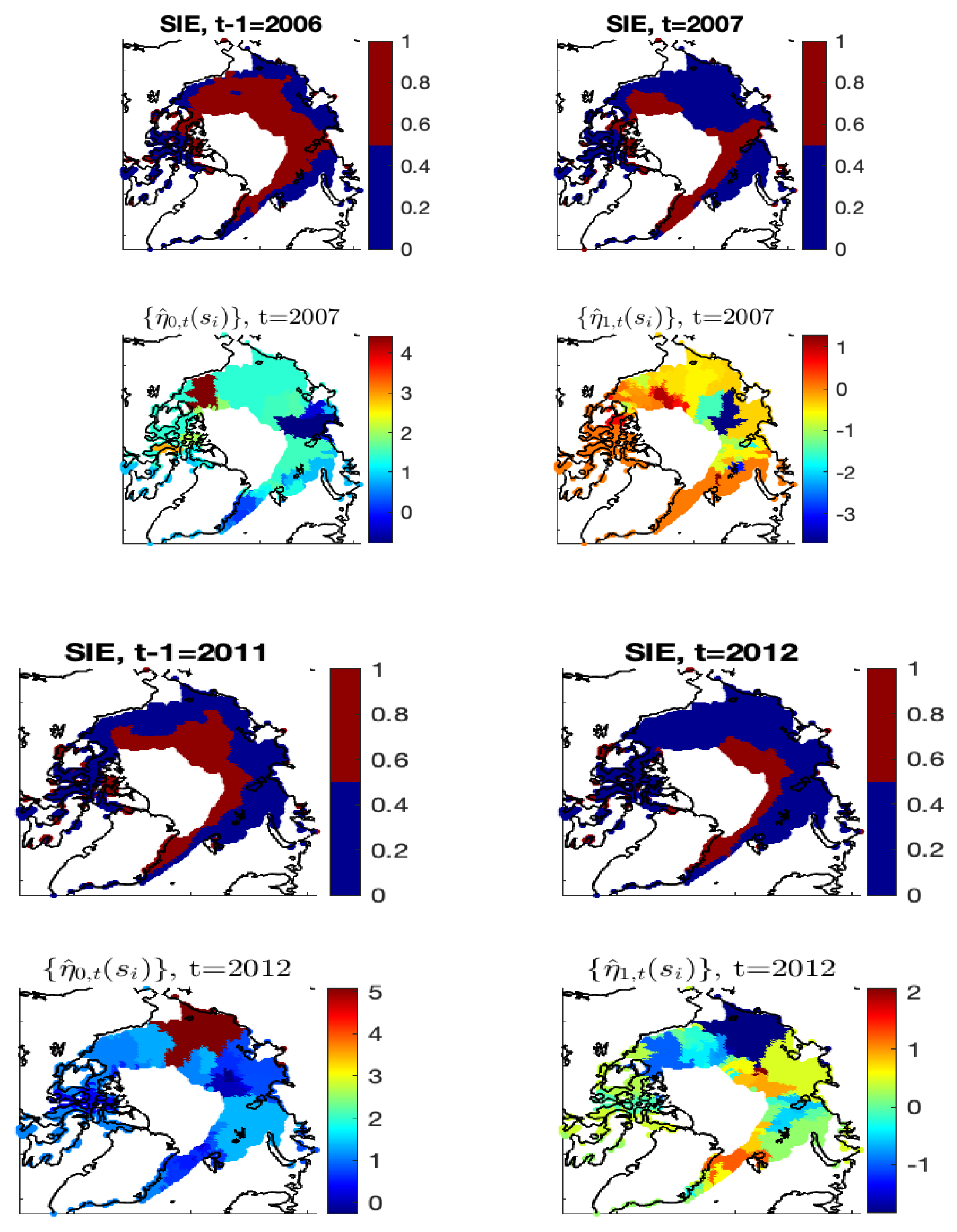
Figure A6 shows the additional estimation results of Model-1c at
and 2012. We can see that the fitted results from Model-1c are reasonable, resulting in the estimated ice probabilities behaving similarly to the Arctic SIE data. The corresponding estimates of the autoregressive coefficients are shown in
Figure A7, whose values adapt well to the observed ice–water/water–ice transitions in regions with substantial loss or gain of sea ice from
to
t.
Figure A6.
Years 2007 and 2012 are shown. Left panels: The estimates . Middle panels: The estimates using a cut-off value to dichotomize . Right panels: The binary Arctic sea ice data derived from satellite data.
Figure A6.
Years 2007 and 2012 are shown. Left panels: The estimates . Middle panels: The estimates using a cut-off value to dichotomize . Right panels: The binary Arctic sea ice data derived from satellite data.
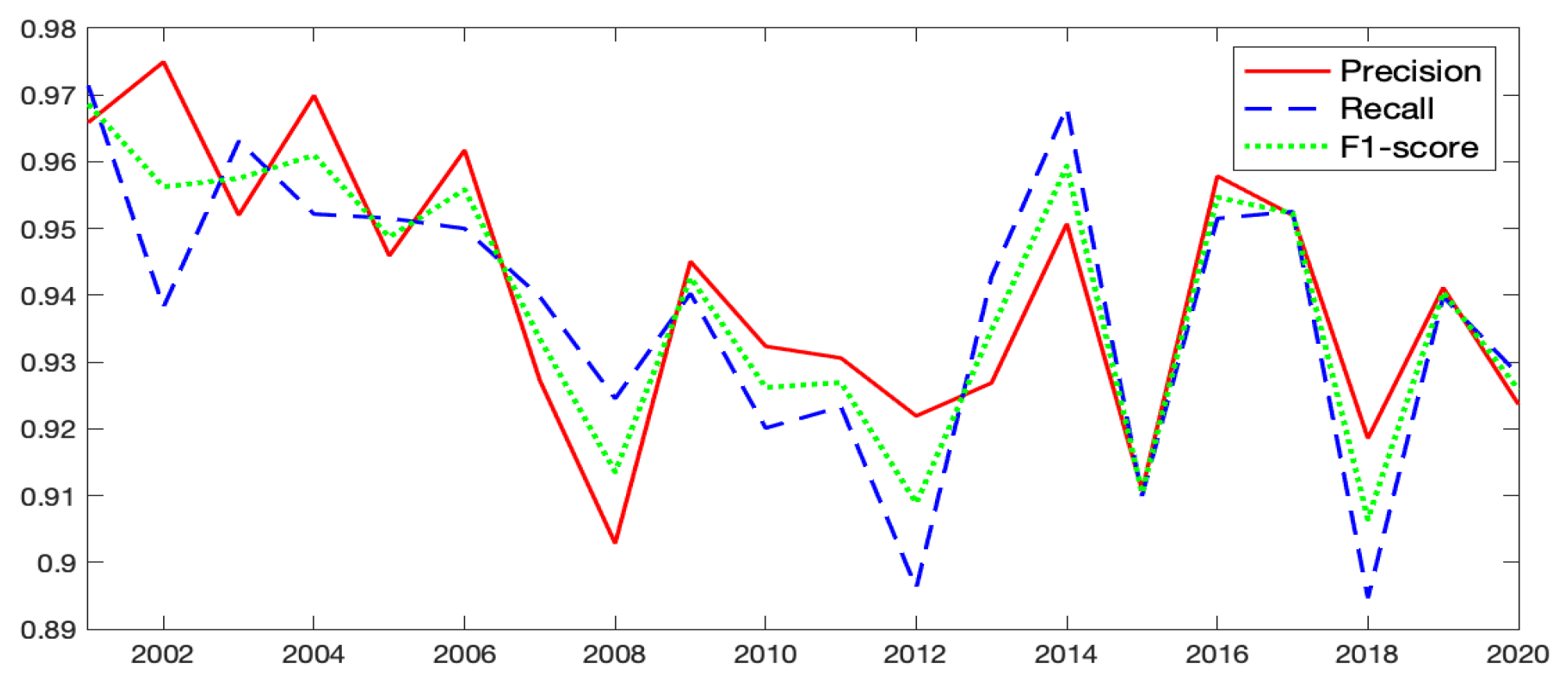
The time-averaged
confusion matrix is given in
Table A4. The number of misclassified ice grid cells and the number of misclassified water grid cells are roughly balanced. The time-averaged correct classification rate for ice is
, which is very close to that for water (
). We further calculated several parameters of the confusion matrix for the selected Model-1c, including precision, recall (sensitivity), and F1-score. Precision is the proportion of correctly classified ice grid cells among all the classified ice grid cells by the model, recall is the proportion of correctly classified ice grid cells among all the observed ice grid cells, and F1-score is the harmonic mean of precision and recall.
Figure A7.
Spatial maps of the observed ice/water statuses at and t and the autoregressive-coefficient estimates and of Model-1c, for and .
Figure A7.
Spatial maps of the observed ice/water statuses at and t and the autoregressive-coefficient estimates and of Model-1c, for and .
Table A4.
Time-averaged confusion matrix for Model-1c.
Table A4.
Time-averaged confusion matrix for Model-1c.
| | |
|---|
| (actual ice) | | |
| (actual water) | | |
The corresponding time series plots of those parameters for Model-1c are shown in
Figure A8. The time series of the precision, recall, and F1-score parameters have fluctuations over years, with values generally above
. We find that relatively lower values of precision and recall occur at years when the overall sea ice patterns are largely different between
and
t (e.g.,
and 2018). This may be because when the sea ice patterns change dramatically from
to
t, it will be difficult to borrow last year’s sea ice information to estimate the presence of sea ice in the current year.
Figure A8.
The time series of precision, recall, and F1-score parameters of the confusion matrix for Model-1c.
Figure A8.
The time series of precision, recall, and F1-score parameters of the confusion matrix for Model-1c.
Last, we have conducted an experiment to test the spatial prediction performance of Model-1c. Specifically, we randomly split the data locations into a training set with 7806 locations and a testing set with 867 locations; the training set contains about
of the total locations, and the testing set contains the remaining
. At each time point
t, we first estimated the model parameters based on the training data, and spatial predictions were conducted subsequently by (i) obtaining the autoregressors for each testing location
using its 8 nearest neighboring training data at time
and (ii) plugging in the estimated model coefficients corresponding to the training data that are nearest to
. In this way, we can obtain estimated ice probabilities for the testing data. The following
Table A5 gives the time-averaged model evaluation scores of Model-1c on both the training and testing data. We can see that the estimation results for the best model (Model-1c) are still reasonable, with the three model evaluation scores for the testing data close to those for the training data.
Table A5.
Time-averaged model evaluation scores: The mean squared errors (MSEs), Nash–Sutcliffe model efficiency coefficients (NSEs), and the correct classification rates (CRs) for Model-1c.
Table A5.
Time-averaged model evaluation scores: The mean squared errors (MSEs), Nash–Sutcliffe model efficiency coefficients (NSEs), and the correct classification rates (CRs) for Model-1c.
| Model-1c | MSE | NSE | CR |
|---|
| Training | | | |
| Testing | | | |
Conclusion. Our conclusion is that Model-1c, namely, the model given by (
3) in the paper, is the best model. Its estimates give superior model evaluation scores, and hence those estimates are used to compute the summaries and their visualization of the spatio-temporal variability in Arctic sea ice.
Uncertainty Estimation. The parametric bootstrap method, e.g., [
54] provides a feasible way for obtaining the standard errors of
for Model-1c. Let
denote the parameter estimates of Model-1c at time
t. The bootstrap samples can be generated in the following manner. At the initial time
, the estimates
are plugged into equation (
3) to obtain the estimated ice probabilities
, and the bootstrap samples,
, are independently generated from the Bernoulli distributions with parameters
. Then, starting from
, the bootstrap samples at time
t are generated by (i) constructing the autoregressors using the bootstrap samples
; (ii) plugging the autoregressors and the parameter estimates
into (
3) to obtain the estimated ice probabilities
; and (iii) generating the bootstrap samples
independently from the Bernoulli distributions with parameters
. This data-generating process is repeated
B times to obtain
B bootstrap samples.
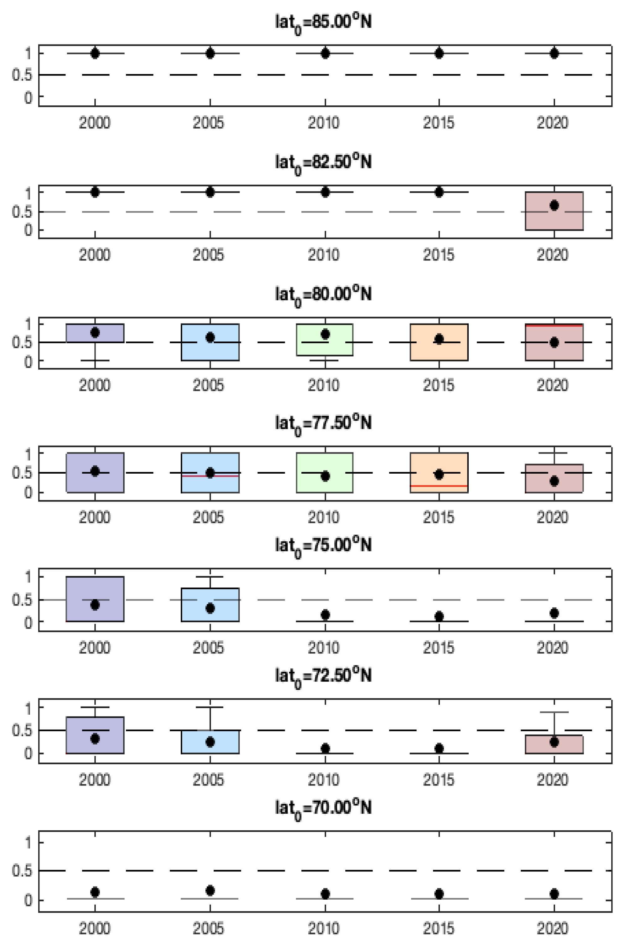
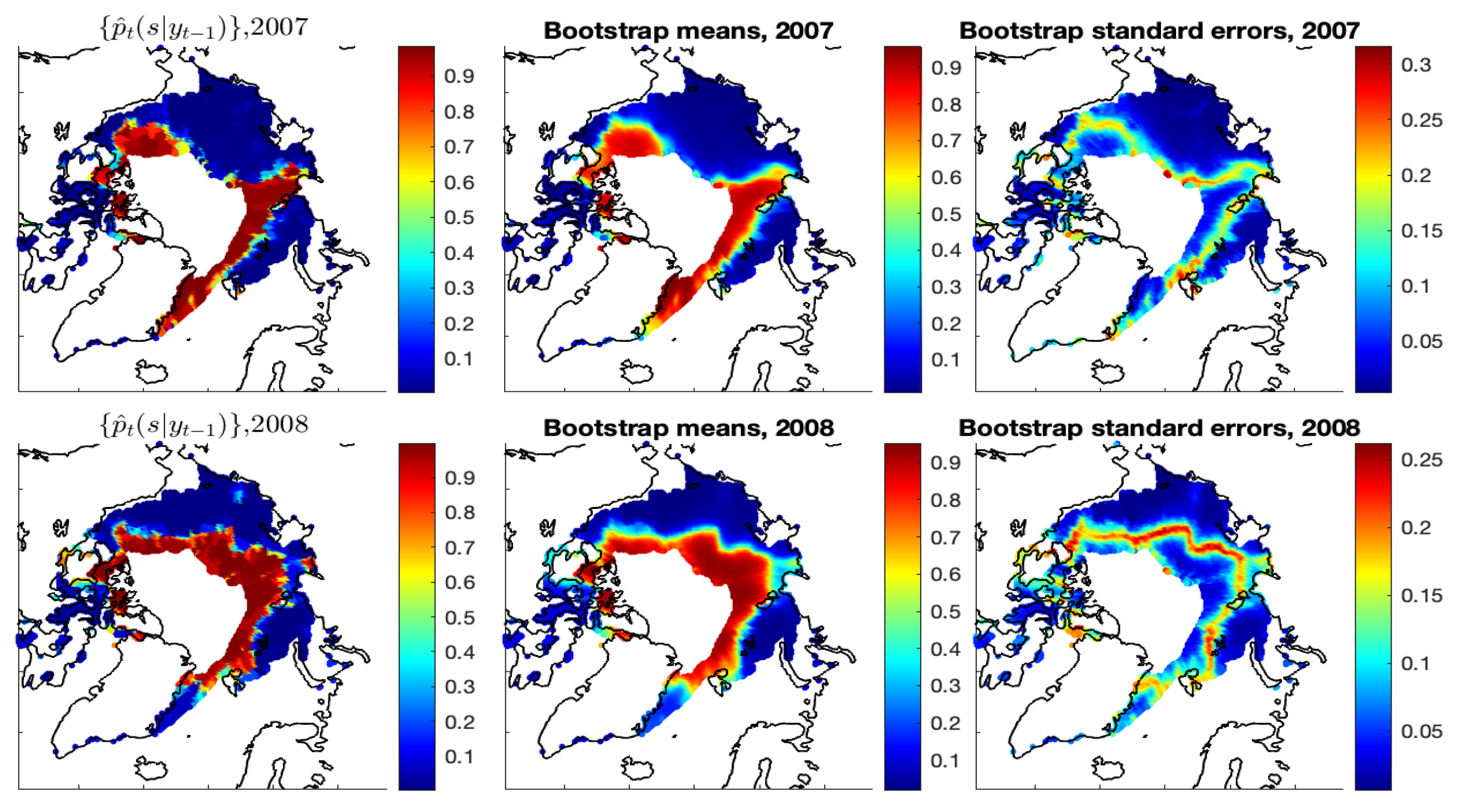
The right panels of
Figure A9 show the bootstrap standard errors of the estimated ice probabilities of Model-1c based on 100 bootstrap samples. We can see that the uncertainties of
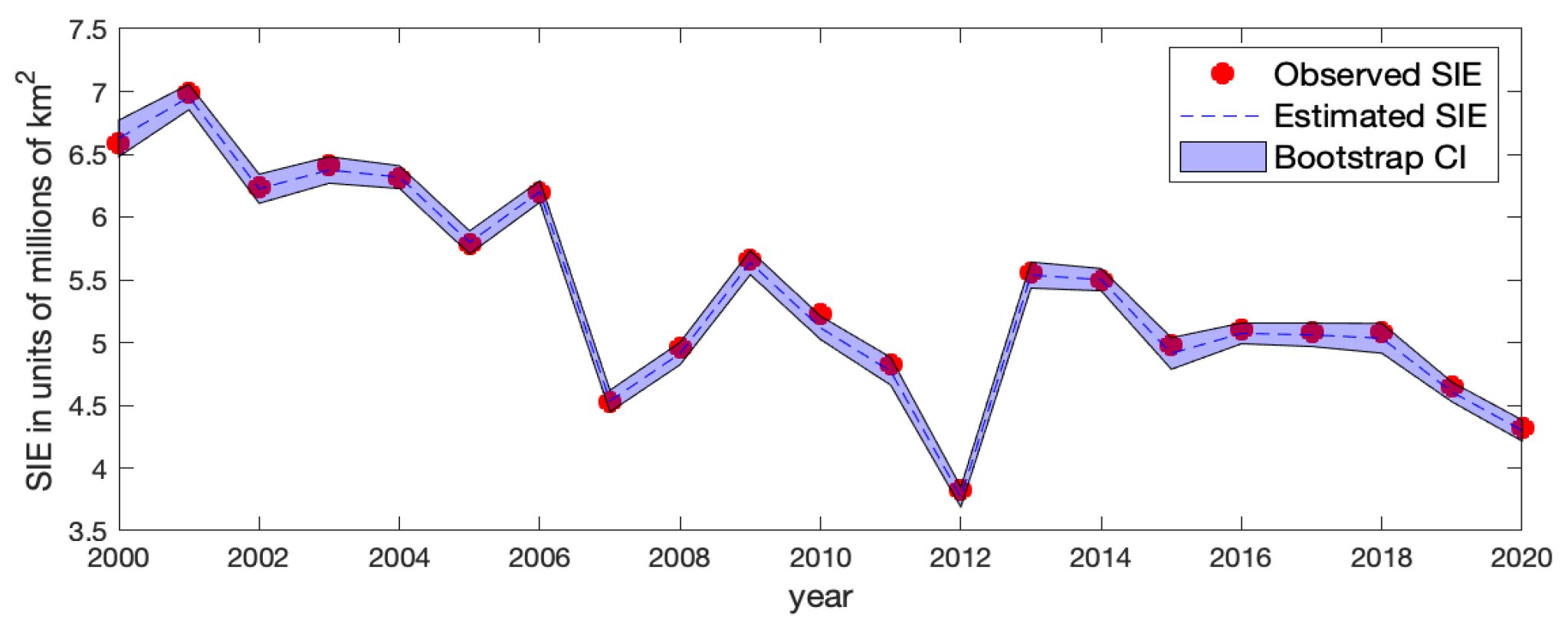
mainly reside in the ice–water boundary regions where classifying ice/water grid cells is more difficult. We also obtained the standard errors of the estimated Arctic SIE based on those bootstrap samples at each year
t. The corresponding approximate
confidence interval of the Arctic SIE is shown in
Figure A10, where at each time
t, the upper and lower limits of the bootstrap confidence interval are equal to the estimated Arctic SIE plus and minus its two bootstrap standard errors, respectively. Values at time
are joined to respective values at time
t by straight lines. The pointwise bootstrap confidence intervals generally cover the observed Arctic SIE values, indicating that the fitting results are reasonable.
Figure A9.
Years 2007 and 2008 are shown. Left panels: The estimates of Model-1c. Middle panels: The bootstrap means of the estimated ice probabilities from 100 bootstrap samples. Right panels: The bootstrap standard errors of the estimated ice probabilities.
Figure A9.
Years 2007 and 2008 are shown. Left panels: The estimates of Model-1c. Middle panels: The bootstrap means of the estimated ice probabilities from 100 bootstrap samples. Right panels: The bootstrap standard errors of the estimated ice probabilities.
Figure A10.
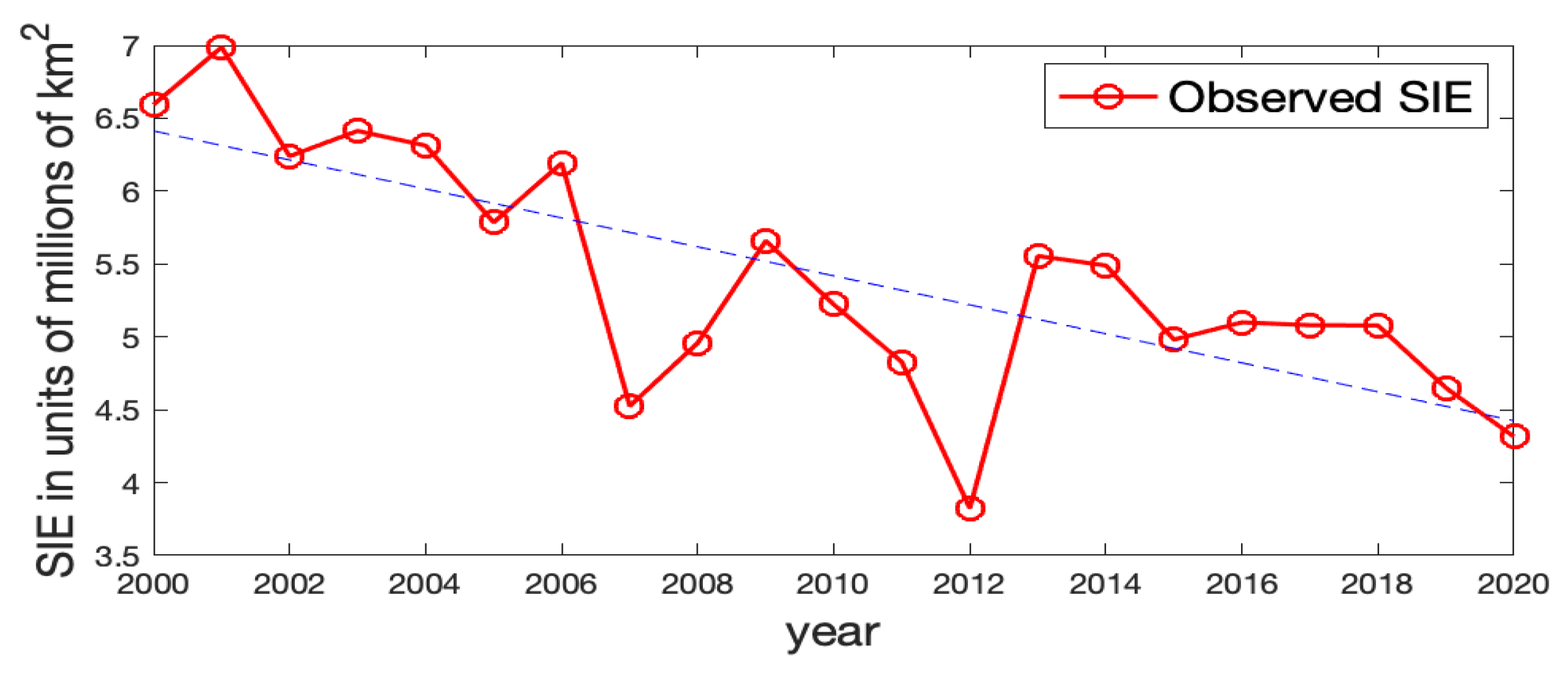
The observed Arctic SIE (red solid dot), the estimated Arctic SIE by Model-1c (blue dashed line), and the bootstrap pointwise confidence interval of the Arctic SIE (shaded blue band).
Figure A10.
The observed Arctic SIE (red solid dot), the estimated Arctic SIE by Model-1c (blue dashed line), and the bootstrap pointwise confidence interval of the Arctic SIE (shaded blue band).


