


Hyperspectral Video Target Tracking Based on Deep Features with Spectral Matching Reduction and Adaptive Scale 3D Hog Features
 ,
,  and
and
Abstract

1. Introduction
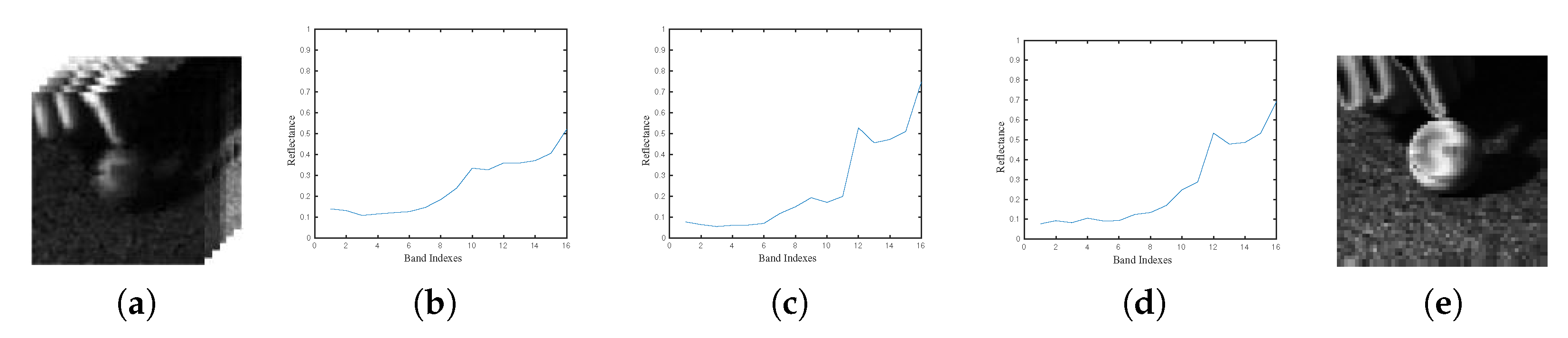
- A spectral matching reduction method is proposed to reduce the dimensionality of the HSI. The proposed method estimates the final spectral curve using the global and local spectral curves. The dimensionality-reduced image is obtained by computing the similarity between final spectral curve, and the spectral curve of each pixel of original image. This approach makes the target more distinguishable from the background and is helpful for subsequent target tracking;
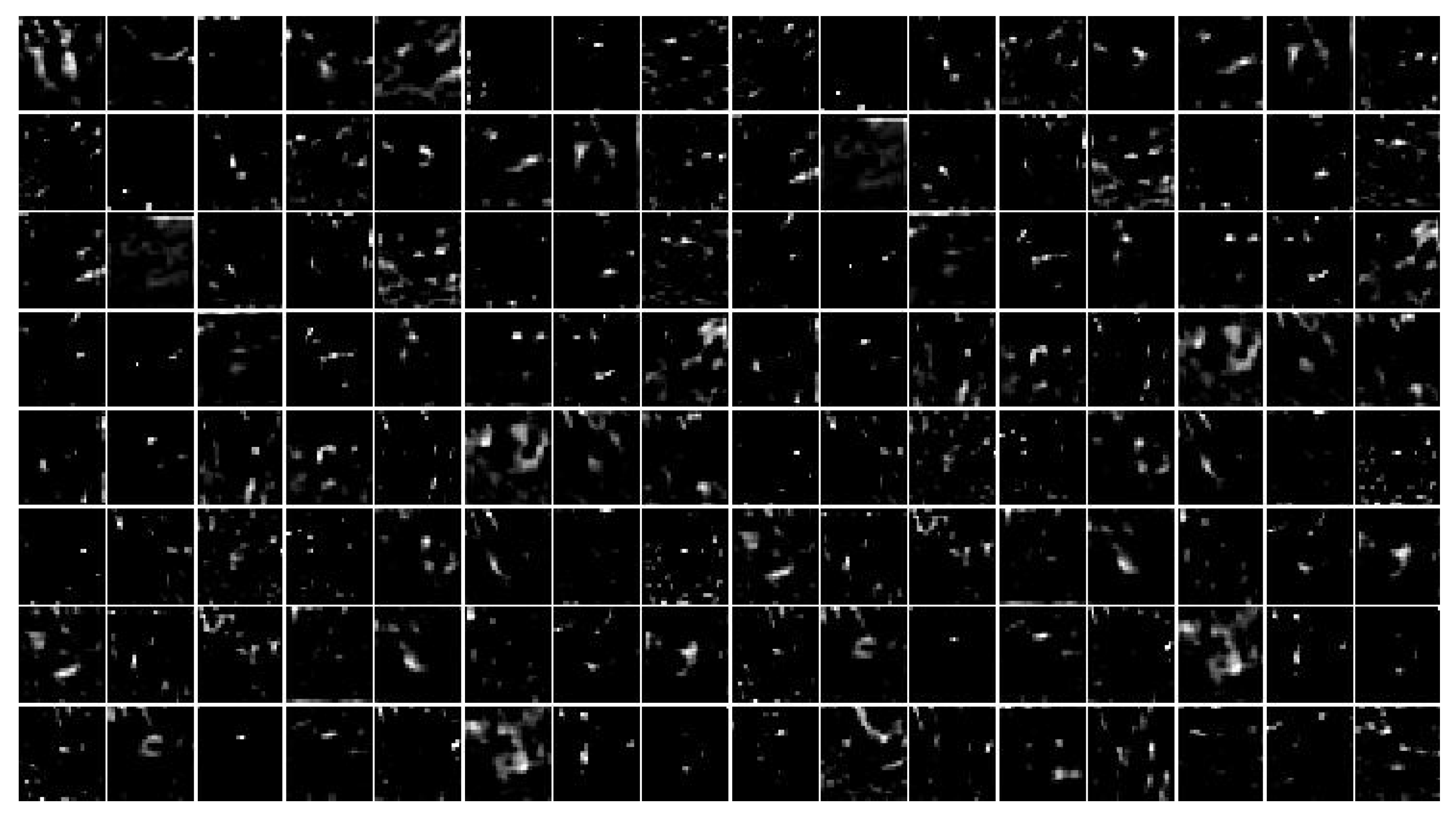
- An AS 3D HOG feature is proposed to extract the 3D HOG features at different scales. The proposed approach ensures robustness against the scale variations of the target while maintaining the original spectral discrimination ability;
- A weighted fusion strategy of feature maps is proposed in which the adaptive weighting coefficients are computed using peak-to-side lobe ratio in the time domain;
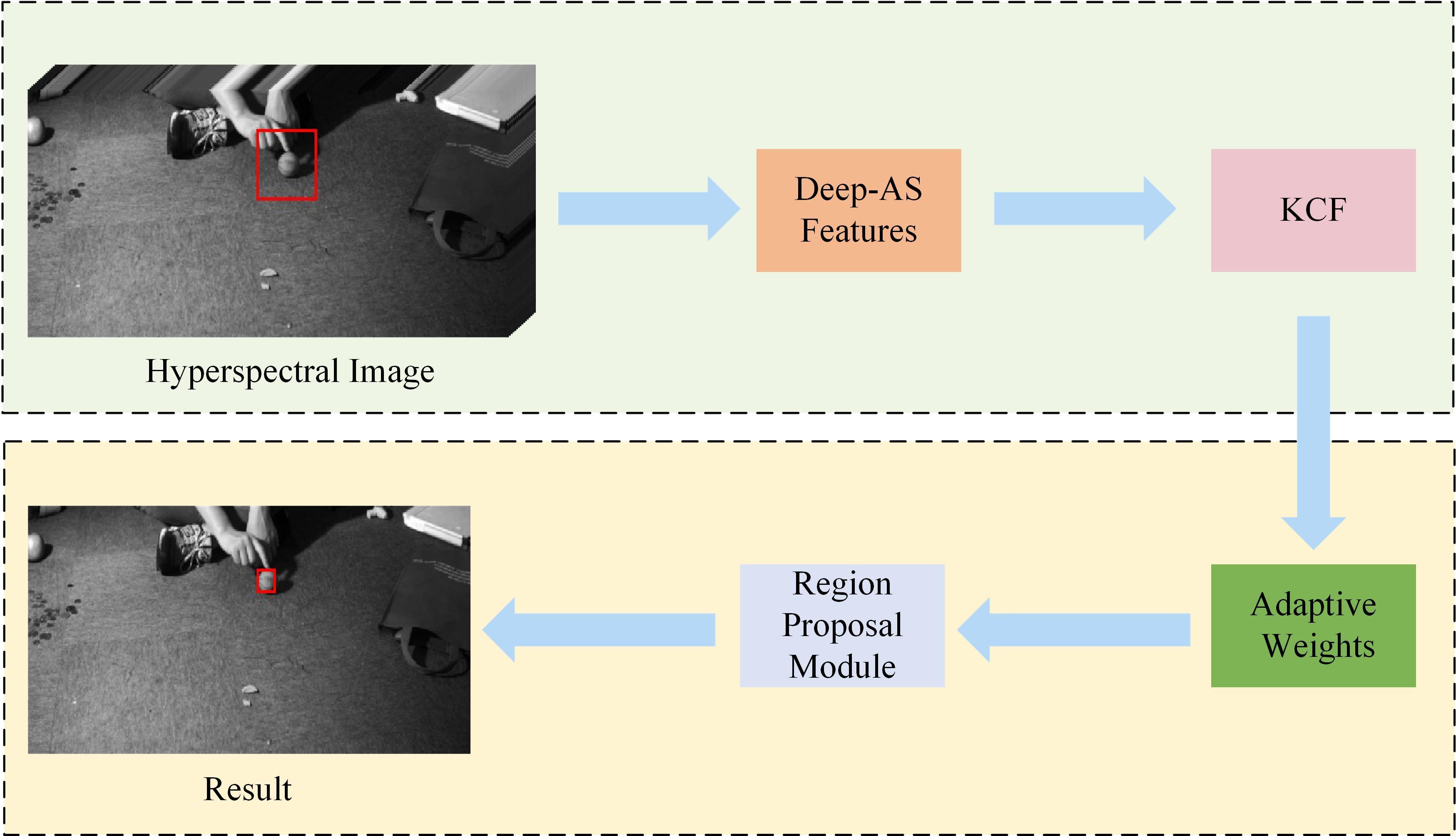
- Inspired by Region Proposal Network (RPN), a novel target box estimation method, named RPM, is proposed. The proposed RPM method can adaptively change the aspect ratio of target box to obtain more accurate box estimation.
2. Related Works
3. Proposed Method
3.1. Spectral Matching Reduction
3.2. Feature Extraction
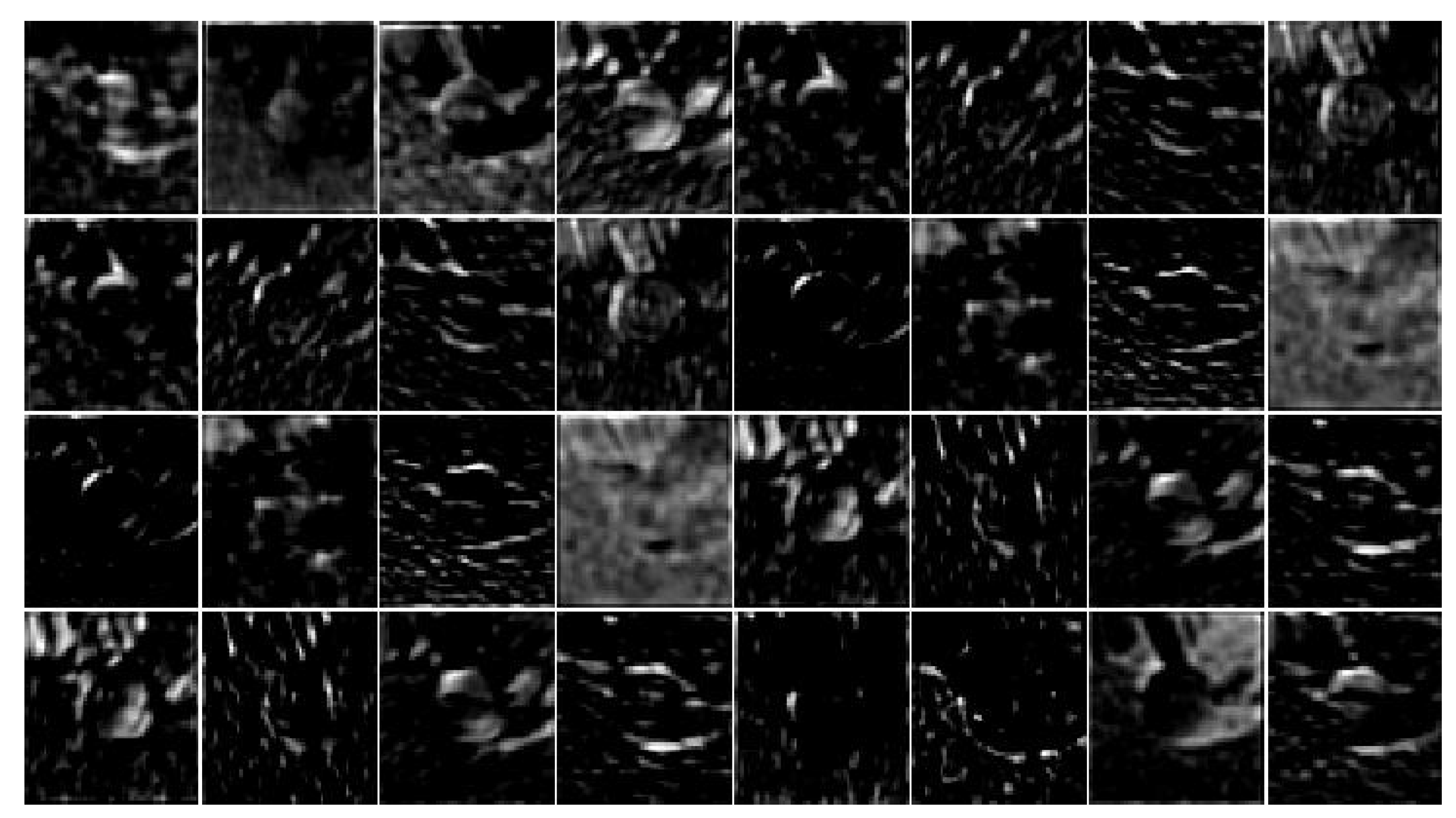
3.2.1. Deep Features
3.2.2. AS 3D Features
3.3. Kernel Correlation Filter
3.4. Target Localization
3.5. Scale Estimation
4. Results and Analysis
4.1. Experiment Setup
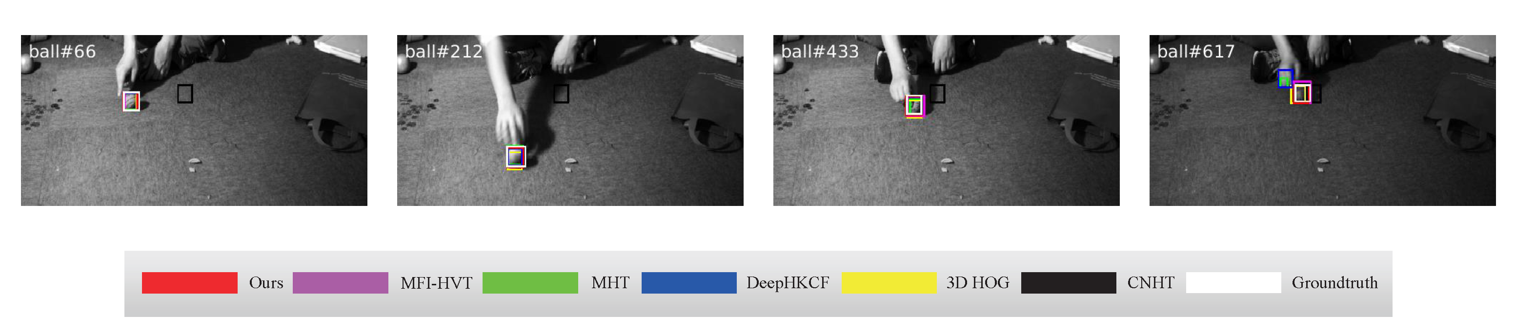
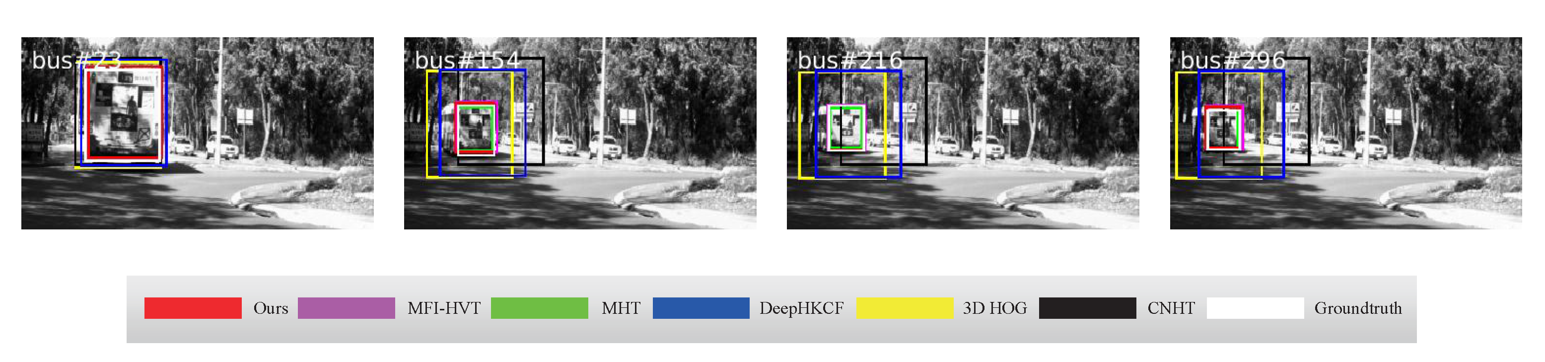
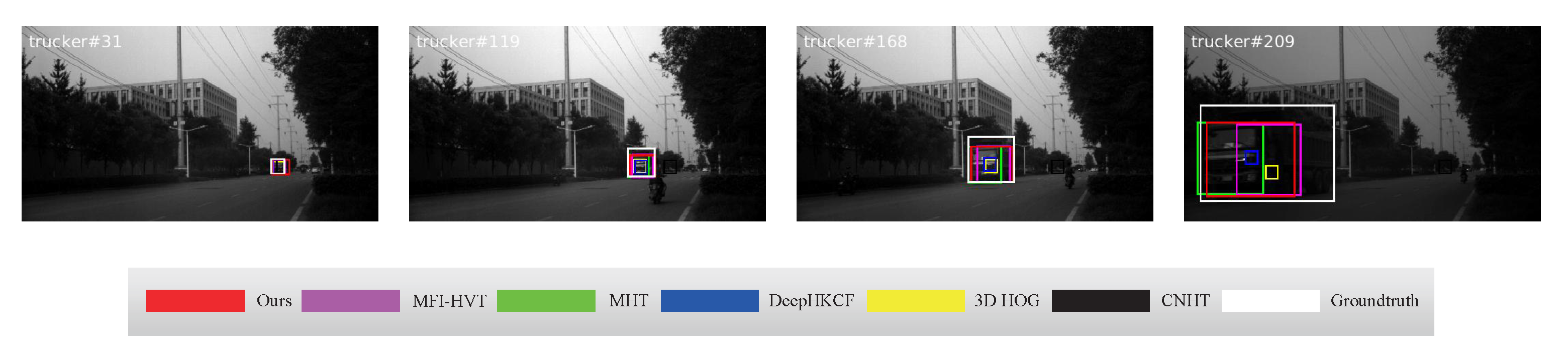
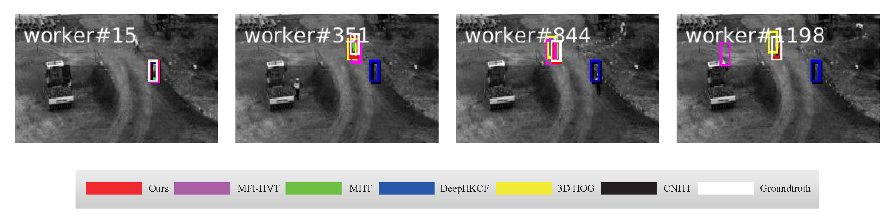
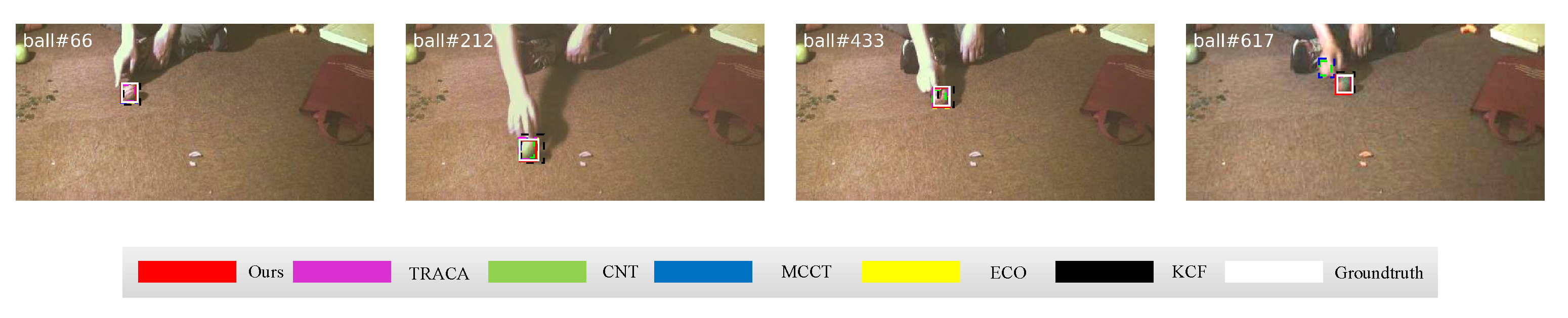
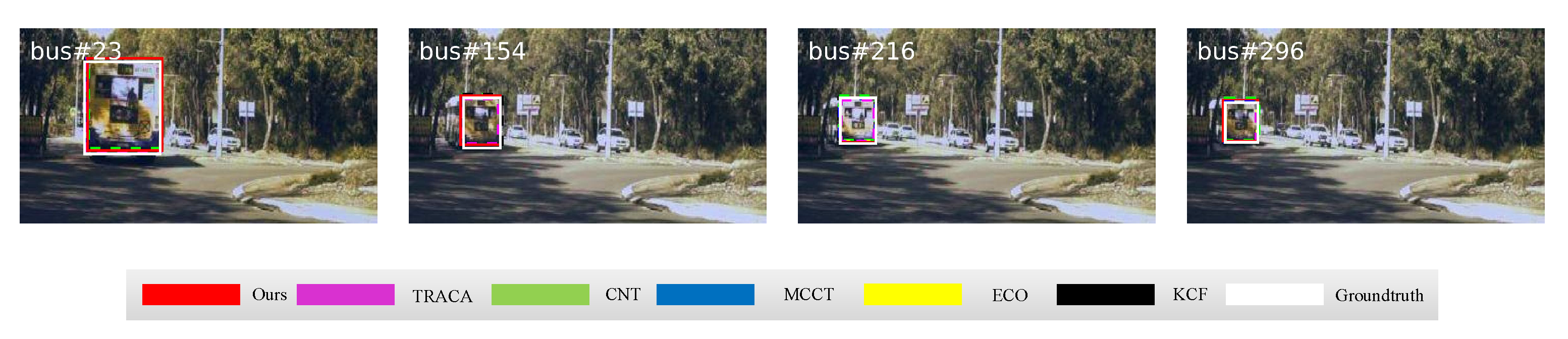
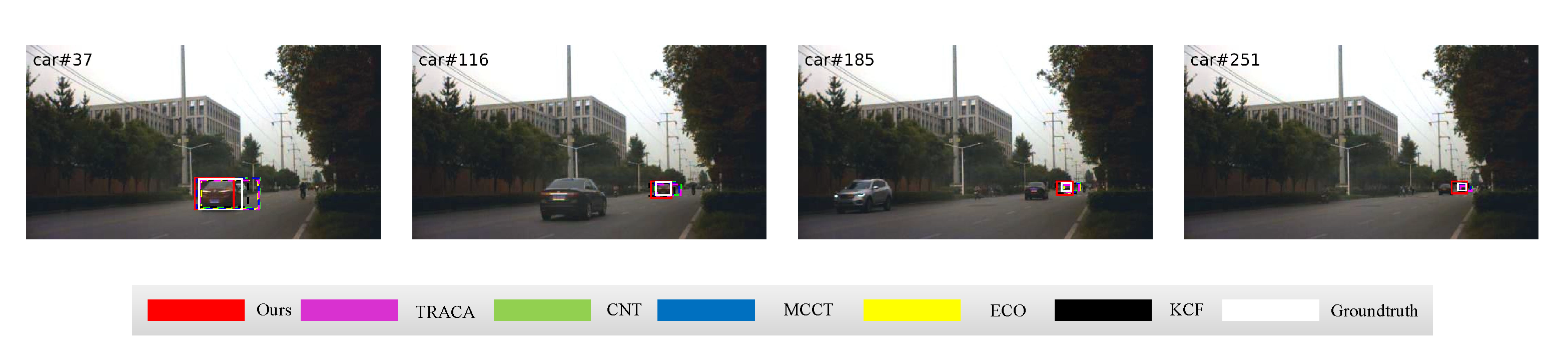
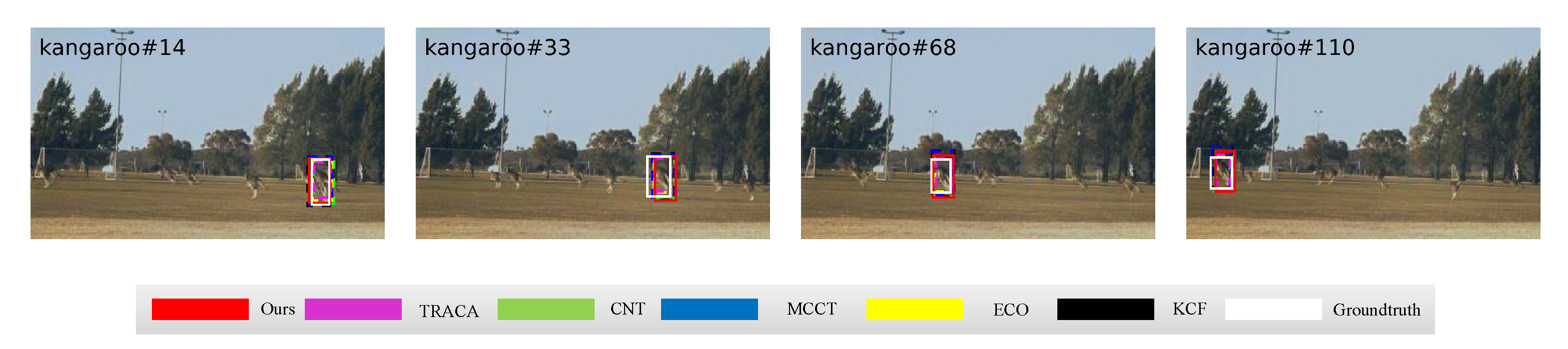
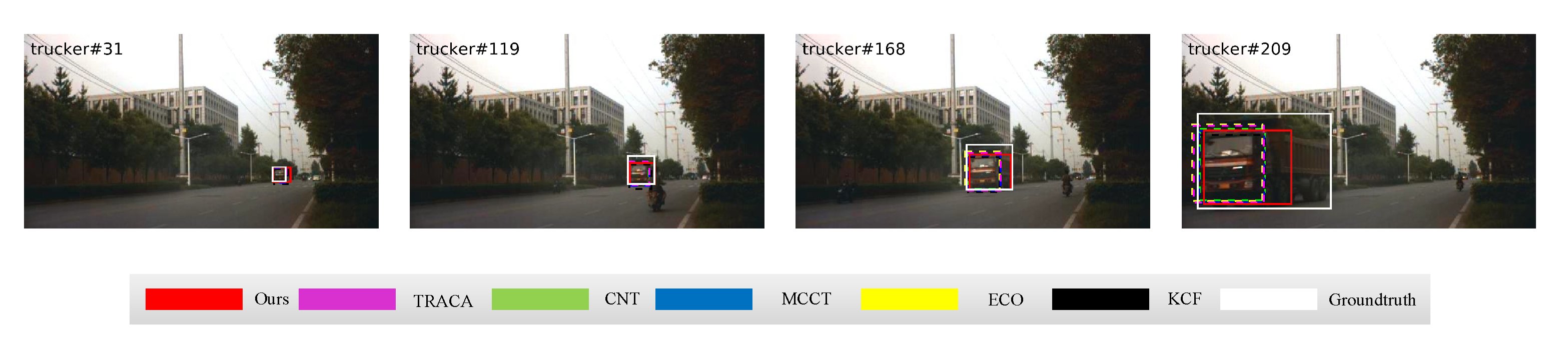
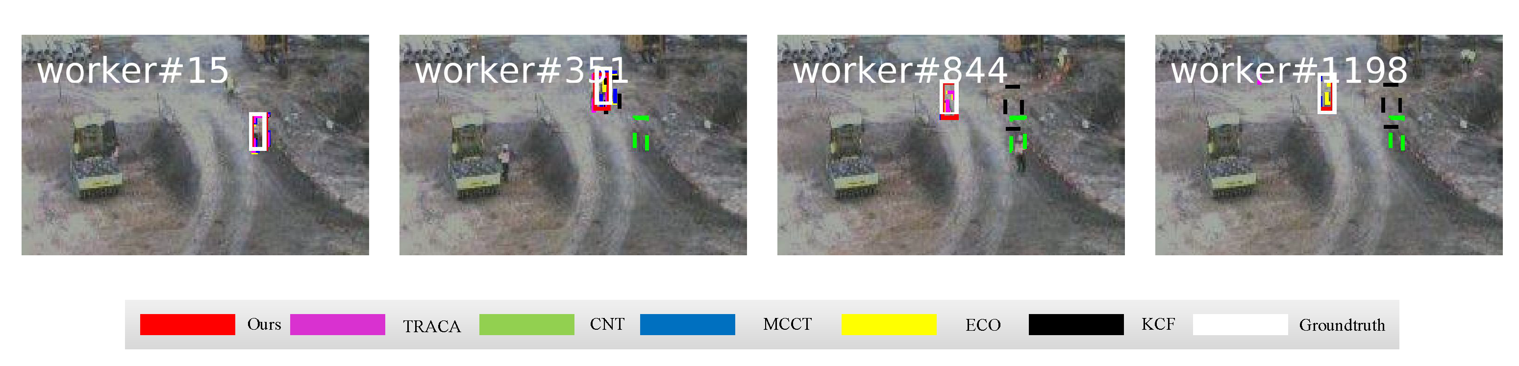
4.2. Qualitative Comparison
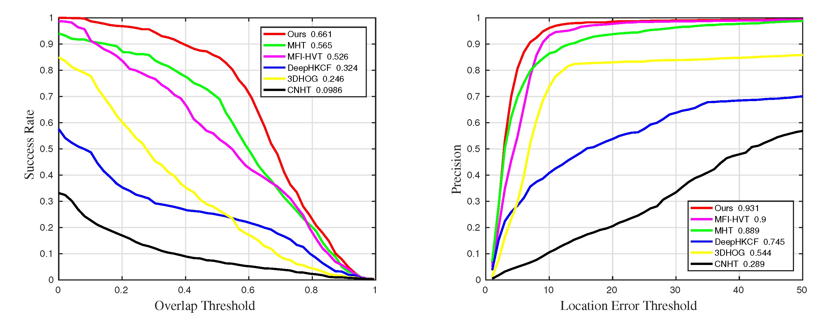
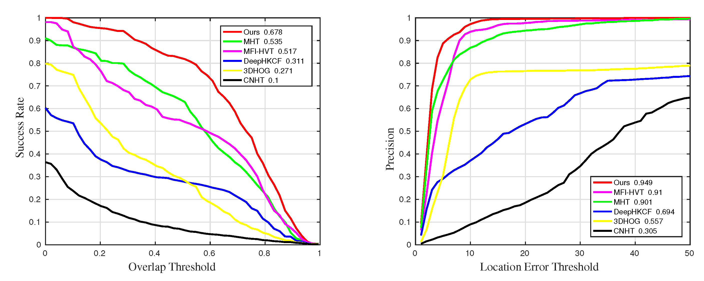
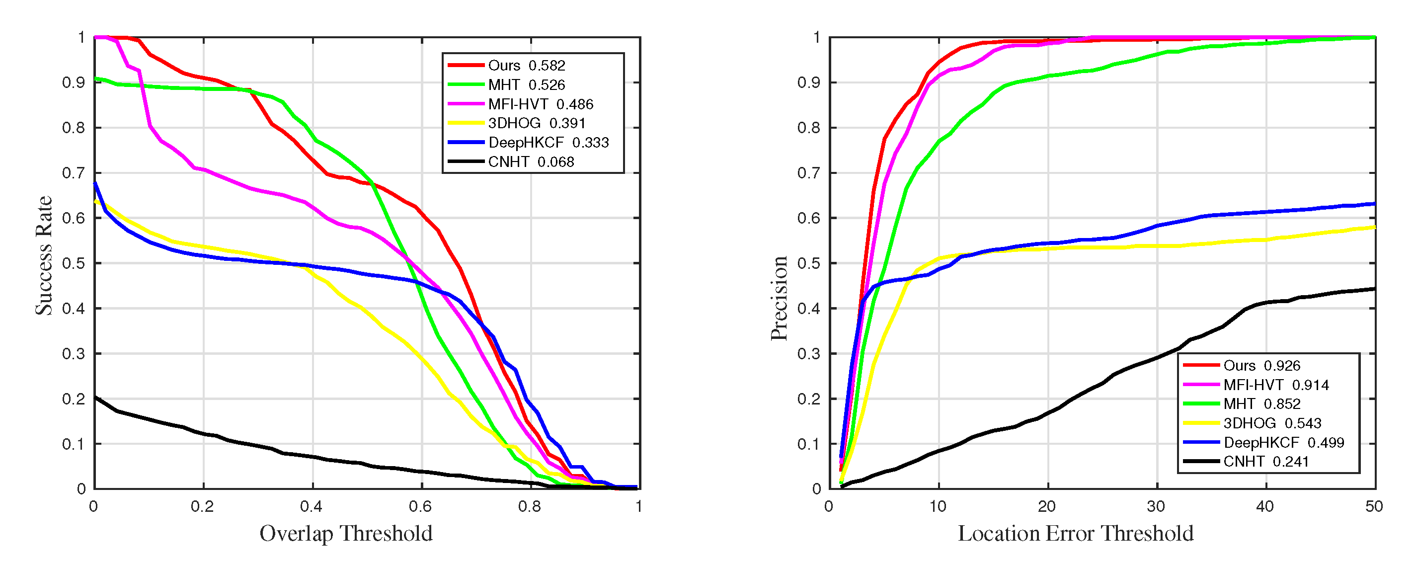
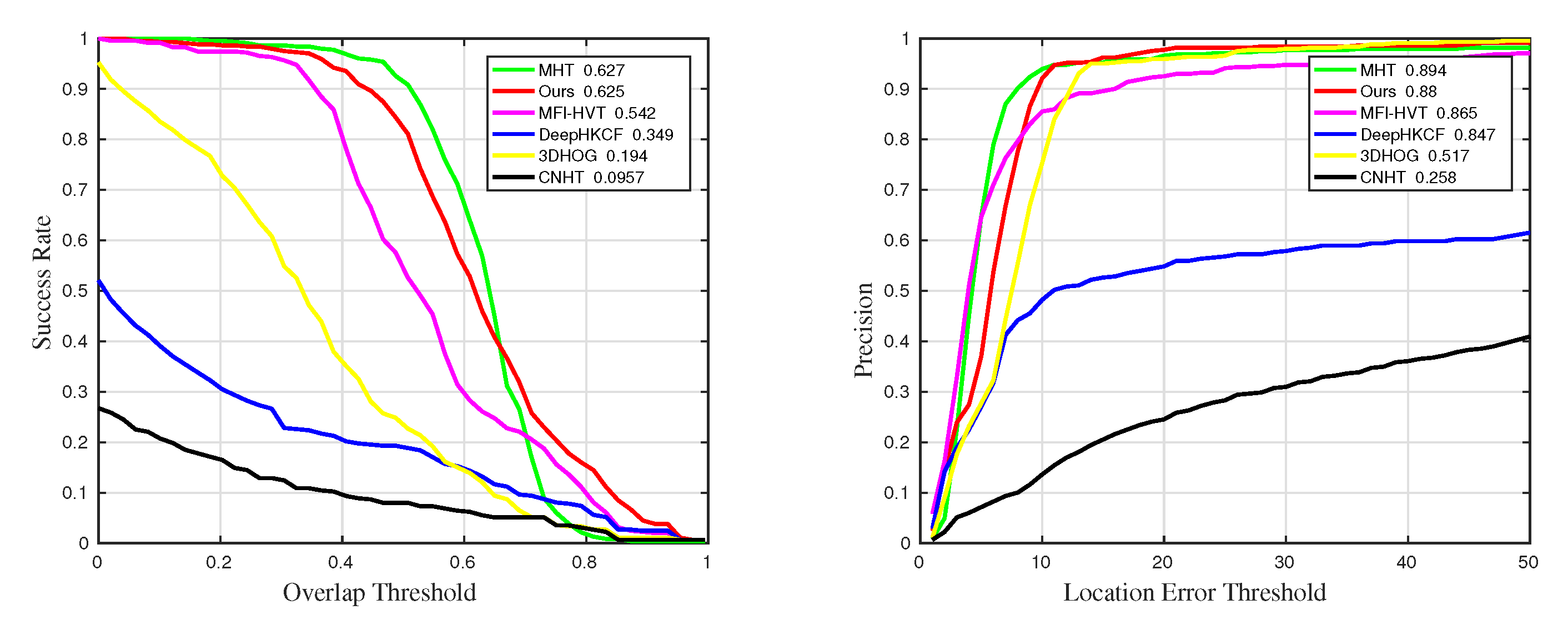
4.3. Quantitative Comparison
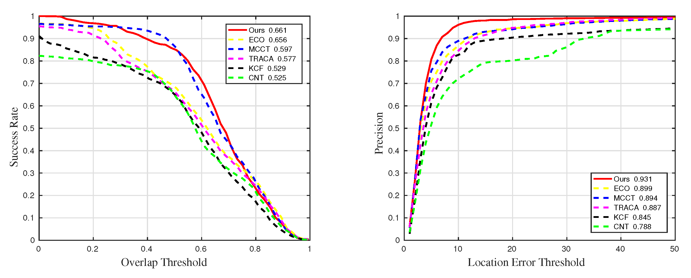
4.4. Comparisons with Color Video Trackers
5. Conclusions
Author Contributions
Funding
Data Availability Statement
Acknowledgments
Conflicts of Interest
References
- Zhao, D.; Gu, L.; Qian, K.; Zhou, H.; Cheng, K. Target tracking from infrared imagery via an improved appearance model. Infrared Phys. Technol. 2019, 104, 103–116. [Google Scholar] [CrossRef]
- Yan, B.; Peng, H.; Wu, K.; Wang, D.; Fu, J.; Lu, H. LightTrack: Finding Lightweight Neural Networks for Object Tracking via One-Shot Architecture Search. In Proceedings of the IEEE Conference on Computer Vision and Pattern Recognition, Nashville, TN, USA, 19–25 June 2021. [Google Scholar]
- Borsuk, V.; Vei, R.; Kupyn, O.; Martyniuk, T.; Krashenyi, I.; Matas, J. FEAR: Fast, Efficient, Accurate and Robust Visual Tracker. In Proceedings of the European Conference on Computer Vision, Tel Aviv, Israel, 23–27 October 2022. [Google Scholar]
- Cao, Z.; Huang, Z.; Pan, L.; Zhang, S.; Liu, Z.; Fu, C. TCTrack: Temporal Contexts for Aerial Tracking. In Proceedings of the IEEE Conference on Computer Vision and Pattern Recognition, New Orleans, LA, USA, 19–24 June 2022. [Google Scholar]
- Danelljan, M.; Häger, G.; Khan, F.S.; Felsberg, M. Adaptive Decontamination of the Training Set: A Unified Formulation for Discriminative Visual Tracking. In Proceedings of the IEEE Conference on Computer Vision and Pattern Recognition, Las Vegas, NV, USA, 27–30 June 2016. [Google Scholar]
- Feng, W.; Han, R.; Guo, Q.; Zhu, J.; Wang, S. Dynamic Saliency-Aware Regularization for Correlation Filter-Based Object Tracking. IEEE Trans. Image Process. 2019, 28, 3232–3245. [Google Scholar] [CrossRef] [PubMed]
- Li, Y.; Xie, W.; Li, H. Hyperspectral image reconstruction by deep convolutional neural network for classification. Pattern Recognit. 2017, 63, 371–383. [Google Scholar] [CrossRef]
- Song, S.; Zhou, H.; Yang, Y.; Song, J. Hyperspectral Anomaly Detection via Convolutional Neural Network and Low Rank with Density-Based Clustering. IEEE J. Sel. Top. Appl. Earth Obs. Remote Sens. 2019, 12, 3637–3649. [Google Scholar] [CrossRef]
- Liang, J.; Zhou, J.; Tong, L.; Bai, X.; Wang, B. Material based salient object detection from hyperspectral images. Pattern Recognit. J. Pattern Recognit. Soc. 2018, 76, 476–490. [Google Scholar] [CrossRef]
- Chang, C.I.; Su, W. Constrained band selection for hyperspectral imagery. IEEE Trans. Geosci. Remote Sens. 2006, 44, 1575–1585. [Google Scholar] [CrossRef]
- Kim, J.H.; Kim, J.; Yang, Y.; Kim, S.; Kim, H.S. Covariance-based band selection and its application to near-real-time hyperspectral target detection. Opt. Eng. 2017, 56, 053101. [Google Scholar] [CrossRef]
- Yang, C.; Bruzzone, L.; Zhao, H.; Tan, Y.; Guan, R. Superpixel-Based Unsupervised Band Selection for Classification of Hyperspectral Images. IEEE Trans. Geosci. Remote Sens. 2018, 56, 7230–7245. [Google Scholar] [CrossRef]
- Jolliffe, I.T. Principal Component Analysis. J. Mark. Res. 2002, 87, 513. [Google Scholar]
- Villa, A.; Chanussot, J.; Jutten, C.; Benediktsson, J.A. On the use of ICA for hyperspectral image analysis. In Proceedings of the IEEE International Geoscience and Remote Sensing Symposium, Cape Town, South Africa, 12–17 July 2009. [Google Scholar]
- Green, A.A.; Berman, M.; Switzer, P.; Craig, M. A transformation for ordering multispectral data in terms of image quality with implications for noise removal. IEEE Trans. Geosci. Remote Sens. 1988, 26, 65–74. [Google Scholar] [CrossRef]
- Nielsen, A.A. Kernel Maximum Autocorrelation Factor and Minimum Noise Fraction Transformations. IEEE Trans. Image Process. 2011, 20, 612–624. [Google Scholar] [CrossRef] [PubMed]
- Xia, J.; Falco, N.; Benediktsson, J.A.; Du, P.; Chanussot, J. Hyperspectral Image Classification with Rotation Random Forest Via KPCA. IEEE J. Sel. Top. Appl. Earth Obs. Remote Sens. 2017, 10, 1601–1609. [Google Scholar] [CrossRef]
- Rasti, B.; Ulfarsson, M.O.; Sveinsson, J.R. Hyperspectral Feature Extraction Using Total Variation Component Analysis. IEEE Trans. Geosci. Remote Sens. 2016, 54, 6976–6985. [Google Scholar] [CrossRef]
- Bandos, T.V.; Bruzzone, L.; Camps-Valls, G. Classification of Hyperspectral Images With Regularized Linear Discriminant Analysis. IEEE Trans. Geosci. Remote Sens. 2009, 47, 862–873. [Google Scholar] [CrossRef]
- Li, J.; Qian, Y. Dimension reduction of hyperspectral images with sparse linear discriminant analysis. In Proceedings of the Geoscience and Remote Sensing Symposium, Vancouver, BC, Canada, 24–29 July 2011. [Google Scholar]
- Zhang, L.; Zhang, L.; Bo, D. Deep Learning for Remote Sensing Data: A Technical Tutorial on the State of the Art. IEEE Geosci. Remote Sens. Mag. 2016, 4, 22–40. [Google Scholar] [CrossRef]
- Li, S.; Song, W.; Fang, L.; Chen, Y.; Benediktsson, J.A. Deep Learning for Hyperspectral Image Classification: An Overview. IEEE Trans. Geosci. Remote Sens. 2019, 57, 6690–6709. [Google Scholar] [CrossRef]
- Danelljan, M.; Khan, F.S.; Felsberg, M.; Weijer, J. Adaptive Color Attributes for Real-Time Visual Tracking. In Proceedings of the IEEE Conference on Computer Vision and Pattern Recognition, Columbus, OH, USA, 23–28 June 2014. [Google Scholar]
- Henriques, J.F.; Caseiro, R.; Martins, P.; Batista, J. High-Speed Tracking with Kernelized Correlation Filters. IEEE Trans. Pattern Anal. Mach. Intell. 2015, 37, 583–596. [Google Scholar] [CrossRef]
- Bolme, D.S.; Beveridge, J.R.; Draper, B.A.; Lui, Y.M. Visual object tracking using adaptive correlation filters. In Proceedings of the IEEE Conference on Computer Vision and Pattern Recognition, San Francisco, CA, USA, 13–18 June 2010. [Google Scholar]
- Qian, K.; Zhou, J.; Xiong, F.; Zhou, H.; Du, J. Object Tracking in Hyperspectral Videos with Convolutional Features and Kernelized Correlation Filter. In Proceedings of the International Conference on Smart Multimedia, Toulon, France, 24–26 August 2018. [Google Scholar]
- Zhang, K.; Lei, Z.; Yang, M.H.; Zhang, D. Fast Tracking via Spatio-Temporal Context Learning. arXiv 2013, arXiv:1311.1939. [Google Scholar]
- Chao, M.; Huang, J.B.; Yang, X.; Yang, M.H. Hierarchical Convolutional Features for Visual Tracking. In Proceedings of the IEEE International Conference on Computer Vision, Las Vegas, NV, USA, 27–30 June 2016. [Google Scholar]
- Bailer, C.; Pagani, A.; Stricker, D. A Superior Tracking Approach: Building a Strong Tracker through Fusion. In Proceedings of the European Conference on Computer Vision, Zurich, Switzerland, 6–12 September 2014. [Google Scholar]
- Zhang, J.; Ma, S.; Sclaroff, S. MEEM: Robust Tracking via Multiple Experts Using Entropy Minimization. In Proceedings of the European Conference on Computer Vision, Zurich, Switzerland, 6–12 September 2014. [Google Scholar]
- Khalid, O.; SanMiguel, J.C.; Cavallaro, A. Multi-Tracker Partition Fusion. IEEE Trans. Circuits Syst. Video Technol. 2017, 27, 1527–1539. [Google Scholar] [CrossRef]
- Ning, W.; Zhou, W.; Qi, T.; Hong, R.; Li, H. Multi-Cue Correlation Filters for Robust Visual Tracking. In Proceedings of the IEEE Conference on Computer Vision and Pattern Recognition, Salt Lake City, UT, USA, 18–23 June 2018. [Google Scholar]
- Xiong, F.; Zhou, J.; Qian, Y. Material Based Object Tracking in Hyperspectral Videos. IEEE Trans. Image Process. 2020, 29, 3719–3733. [Google Scholar] [CrossRef]
- Chen, L.; Zhao, Y.; Yao, J.; Chen, J.; Li, N.; Chan, J.C.W.; Kong, S.G. Object Tracking in Hyperspectral-Oriented Video with Fast Spatial-Spectral Features. Remote Sens. 2021, 13, 1922. [Google Scholar] [CrossRef]
- Chen, L.; Zhao, Y.; Chan, J.C.W.; Kong, S.G. Histograms of oriented mosaic gradients for snapshot spectral image description. ISPRS J. Photogramm. Remote Sens. 2022, 183, 79–93. [Google Scholar] [CrossRef]
- Danelljan, M.; Bhat, G.; Khan, F.S.; Felsberg, M. ECO: Efficient Convolution Operators for Tracking. In Proceedings of the IEEE Conference on Computer Vision and Pattern Recognition, Honolulu, HI, USA, 21–26 July 2017. [Google Scholar]
- Sun, C.; Wang, D.; Lu, H.; Yang, M.H. Correlation Tracking via Joint Discrimination and Reliability Learning. In Proceedings of the IEEE Conference on Computer Vision and Pattern Recognition, Salt Lake City, UT, USA, 18–23 June 2018. [Google Scholar]
- Cen, M.; Jung, C. Fully Convolutional Siamese Fusion Networks for Object Tracking. In Proceedings of the European Conference on Computer Vision, Amsterdam, The Netherlands, 11–14 October 2016. [Google Scholar]
- Bo, L.; Yan, J.; Wei, W.; Zheng, Z.; Hu, X. High Performance Visual Tracking with Siamese Region Proposal Network. In Proceedings of the IEEE Conference on Computer Vision and Pattern Recognition, Salt Lake City, UT, USA, 18–23 June 2018. [Google Scholar]
- Li, B.; Wu, W.; Wang, Q.; Zhang, F.; Xing, J.; Yan, J. SiamRPN++: Evolution of Siamese Visual Tracking with Very Deep Networks. In Proceedings of the IEEE Conference on Computer Vision and Pattern Recognition, Long Beach, CA, USA, 15–20 June 2019. [Google Scholar]
- Wang, Q.; Zhang, L.; Bertinetto, L.; Hu, W.; Torr, P. Fast Online Object Tracking and Segmentation: A Unifying Approach. In Proceedings of the IEEE Conference on Computer Vision and Pattern Recognition, Long Beach, CA, USA, 15–20 June 2019. [Google Scholar]
- Lukezic, A.; Matas, J.; Kristan, M. D3S—A Discriminative Single Shot Segmentation Tracker. In Proceedings of the IEEE Conference on Computer Vision and Pattern Recognition, Seattle, WA, USA, 13–19 June 2020. [Google Scholar]
- Xu, Y.; Wang, Z.; Li, Z.; Yuan, Y.; Yu, G. SiamFC++: Towards Robust and Accurate Visual Tracking with Target Estimation Guidelines. In Proceedings of the Association for the Advance of Artificial Intelligence, New York, NY, USA, 7–12 February 2020. [Google Scholar]
- Chen, X.; Yan, B.; Zhu, J.; Wang, D.; Lu, H. Transformer Tracking. In Proceedings of the IEEE Conference on Computer Vision and Pattern Recognition, Nashville, TN, USA, 20–25 June 2021. [Google Scholar]
- Bhat, G.; Danelljan, M.; Gool, L.V.; Timofte, R. Learning Discriminative Model Prediction for Tracking. In Proceedings of the International Conference on Computer Vision, Seoul, Republic of Korea, 27 October–2 November 2019. [Google Scholar]
- Danelljan, M.; Bhat, G.; Khan, F.S.; Felsberg, M. ATOM: Accurate Tracking by Overlap Maximization. In Proceedings of the IEEE Conference on Computer Vision and Pattern Recognition, Long Beach, CA, USA, 15–20 June 2019. [Google Scholar]
- Yan, B.; Wang, D.; Lu, H.; Yang, X. Alpha-Refine: Boosting Tracking Performance by Precise Bounding Box Estimation. In Proceedings of the IEEE Conference on Computer Vision and Pattern Recognition, Seattle, WA, USA, 13–19 June 2020. [Google Scholar]
- Simonyan, K.; Zisserman, A. Very Deep Convolutional Networks for Large-Scale Image Recognition. arXiv 2014, arXiv:1409.1556. [Google Scholar]
- Krizhevsky, A.; Sutskever, I.; Hinton, G. ImageNet Classification with Deep Convolutional Neural Networks. Adv. Neural Inf. Process. Syst. 2017, 60, 84–90. [Google Scholar] [CrossRef]
- Zhang, Z.; Qian, K.; Du, J.; Zhou, H. Multi-Features Integration Based Hyperspectral Videos Tracker. In Proceedings of the IEEE Workshop on Hyperspectral Image and Signal Processing: Evolution in Remote Sensing, Amsterdam, The Netherlands, 24–26 March 2021. [Google Scholar]
- Uzkent, B.; Rangnekar, A.; Hoffman, M.J. Tracking in Aerial Hyperspectral Videos Using Deep Kernelized Correlation Filters. IEEE Trans. Geosci. Remote Sens. 2019, 57, 449–461. [Google Scholar] [CrossRef]
- Choi, J.; Chang, H.J.; Fischer, T.; Yun, S.; Lee, K.; Jeong, J.; Demiris, Y.; Choi, J.Y. Context-Aware Deep Feature Compression for High-Speed Visual Tracking. In Proceedings of the IEEE Conference on Computer Vision and Pattern Recognition, Salt Lake City, UT, USA, 18–23 June 2018. [Google Scholar]


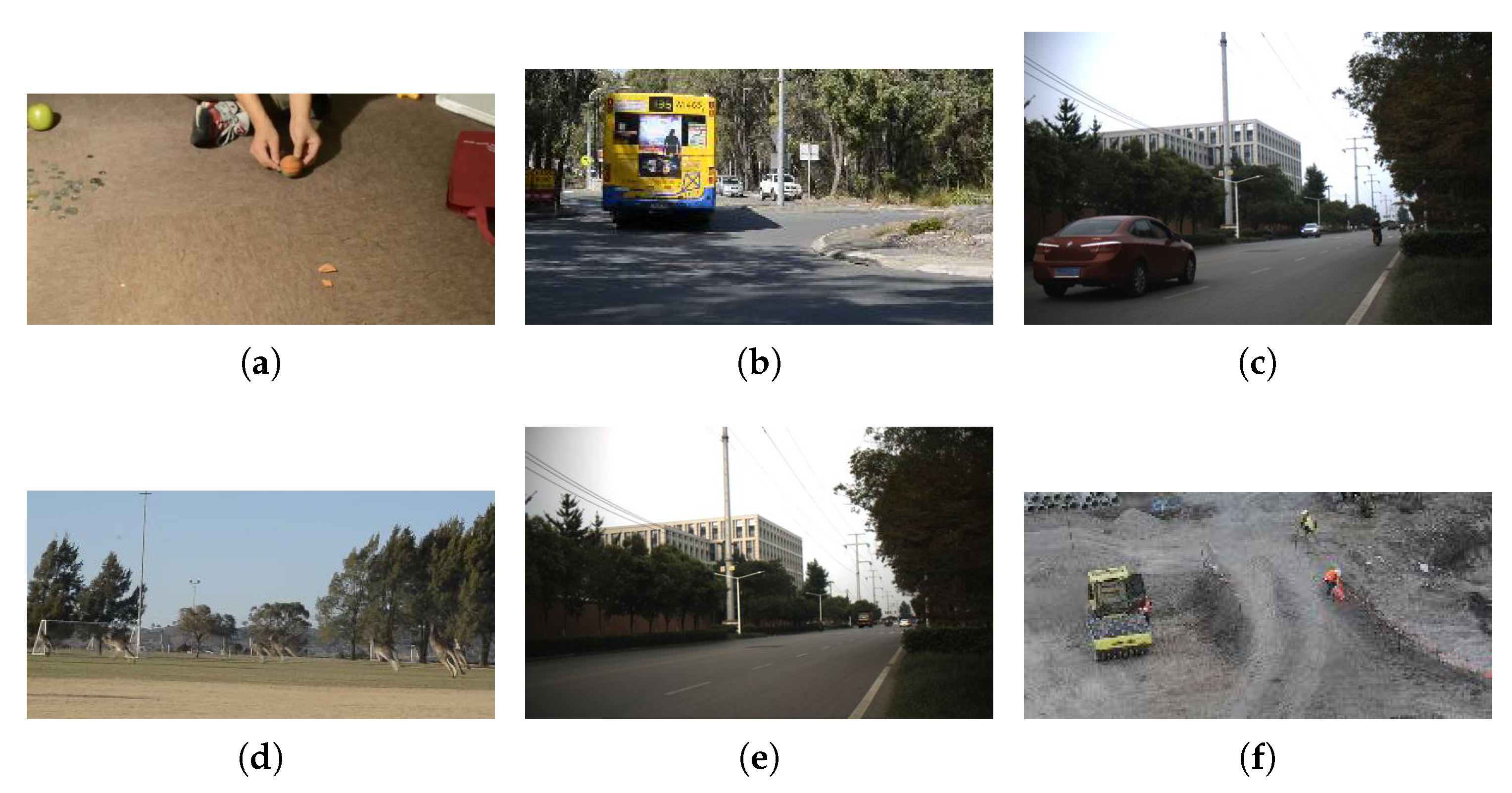
| Sequences | Ball | Bus | Car | Kangaroo | Truck | Worker |
|---|---|---|---|---|---|---|
| Frames | 625 | 326 | 331 | 117 | 221 | 1209 |
| Resolution | ||||||
| Initial Size | ||||||
| Challenges | SV, OCC | SV, FM | SV, OCC | SV, BC | SV, OV | LR, BC |
| Methods | Precision | Precision_SV | Precision_OCC | Precision_BC |
|---|---|---|---|---|
| Ours | ||||
| MHT | 0.889 | 0.901 | 0.852 | |
| MFI-HVT | 0.865 | |||
| DeepHKCF | 0.745 | 0.694 | 0.499 | 0.847 |
| 3DHOG | 0.544 | 0.557 | 0.543 | 0.517 |
| CNHT | 0.289 | 0.305 | 0.241 | 0.258 |
| Methods | Success | Success_SV | Success_OCC | Success_BC |
|---|---|---|---|---|
| Ours | ||||
| MHT | ||||
| MFI-HVT | 0.526 | 0.517 | 0.486 | 0.542 |
| DeepHKCF | 0.324 | 0.311 | 0.333 | 0.349 |
| 3DHOG | 0.246 | 0.271 | 0.391 | 0.194 |
| CNHT | 0.0986 | 0.1 | 0.068 | 0.0957 |
| Methods | Ours | ECO | MCCT | TRACA | KCF | CNT |
|---|---|---|---|---|---|---|
| Precision | 0.894 | 0.887 | 0.845 | 0.788 | ||
| Success | 0.597 | 0.577 | 0.529 | 0.525 |
Publisher’s Note: MDPI stays neutral with regard to jurisdictional claims in published maps and institutional affiliations. |
© 2022 by the authors. Licensee MDPI, Basel, Switzerland. This article is an open access article distributed under the terms and conditions of the Creative Commons Attribution (CC BY) license (https://creativecommons.org/licenses/by/4.0/).
Share and Cite
Zhang, Z.; Zhu, X.; Zhao, D.; Arun, P.V.; Zhou, H.; Qian, K.; Hu, J. Hyperspectral Video Target Tracking Based on Deep Features with Spectral Matching Reduction and Adaptive Scale 3D Hog Features. Remote Sens. 2022, 14, 5958. https://doi.org/10.3390/rs14235958
Zhang Z, Zhu X, Zhao D, Arun PV, Zhou H, Qian K, Hu J. Hyperspectral Video Target Tracking Based on Deep Features with Spectral Matching Reduction and Adaptive Scale 3D Hog Features. Remote Sensing. 2022; 14(23):5958. https://doi.org/10.3390/rs14235958
Chicago/Turabian StyleZhang, Zhe, Xuguang Zhu, Dong Zhao, Pattathal V. Arun, Huixin Zhou, Kun Qian, and Jianling Hu. 2022. "Hyperspectral Video Target Tracking Based on Deep Features with Spectral Matching Reduction and Adaptive Scale 3D Hog Features" Remote Sensing 14, no. 23: 5958. https://doi.org/10.3390/rs14235958
APA StyleZhang, Z., Zhu, X., Zhao, D., Arun, P. V., Zhou, H., Qian, K., & Hu, J. (2022). Hyperspectral Video Target Tracking Based on Deep Features with Spectral Matching Reduction and Adaptive Scale 3D Hog Features. Remote Sensing, 14(23), 5958. https://doi.org/10.3390/rs14235958