
Preflight Evaluation of the Environmental Trace Gases Monitoring Instrument with Nadir and Limb Modes (EMI-NL) Based on Measurements of Standard NO2 Sample Gas


Abstract

1. Introduction
2. Data and Methods
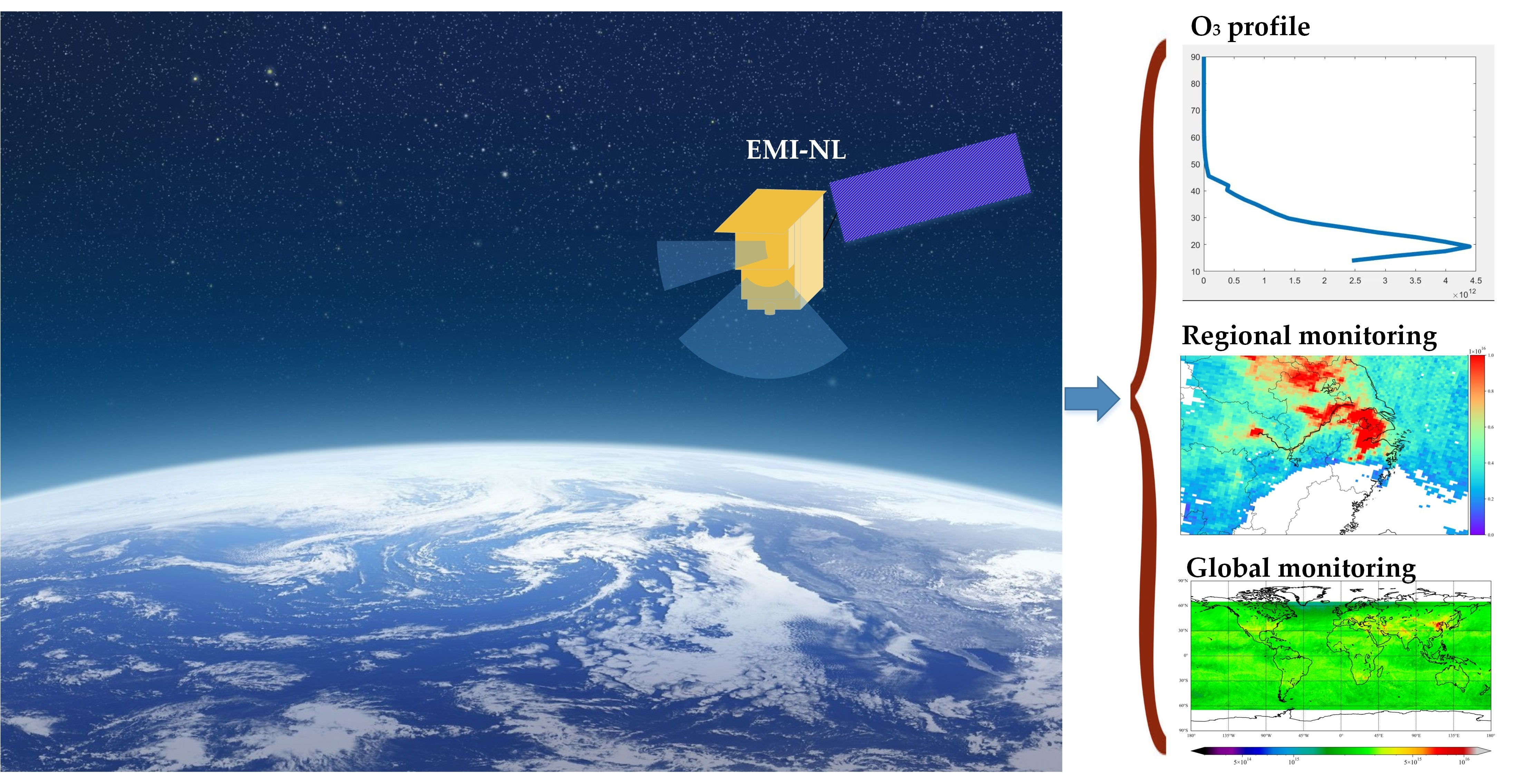
2.1. EMI-NL Description
2.1.1. Nadir Module
2.1.2. Limb Module
2.2. Experimental Design
2.3. DOAS Fitting
2.4. Signal-to-Noise Ratio Estimation
3. Results and Discussion
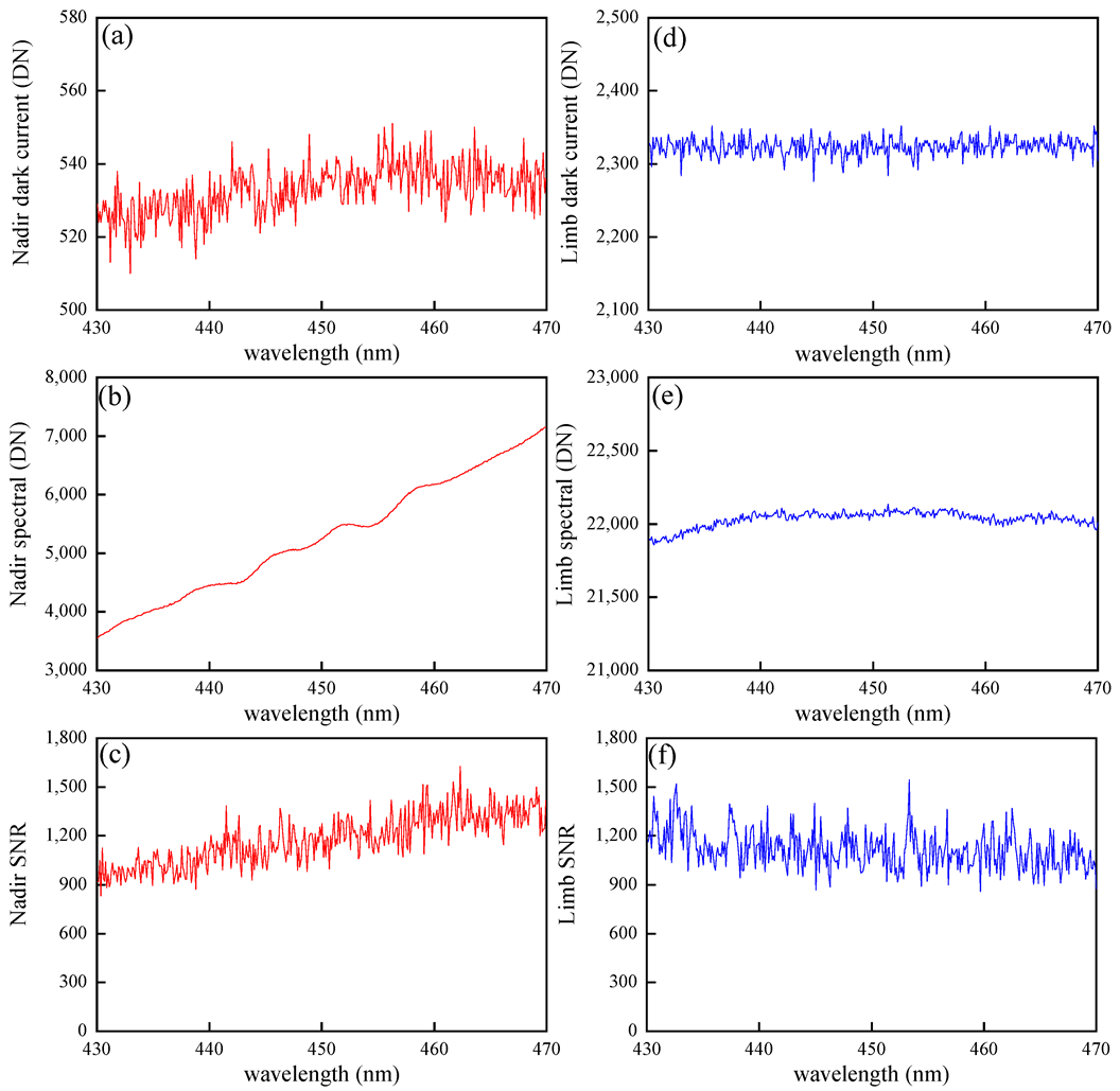
3.1. Results of the Nadir Module
3.2. Results of Limb Module
3.3. Results of SNR Estimation
4. Conclusions
Author Contributions
Funding
Data Availability Statement
Acknowledgments
Conflicts of Interest
References
- Heath, D.F.; Krueger, A.J.; Roeder, H.A.; Henderson, B.D. The Solar Backscatter Ultraviolet and Total Ozone Mapping Spectrometer (SBUV/TOMS) for NIMBUS G. Opt. Eng. 1975, 14, 323–331. [Google Scholar] [CrossRef]
- Burrows, J.P.; Weber, M.; Buchwitz, M.; Rozanov, V.; Ladstatter-Weissenmayer, A.; Richter, A.; de Beek, R.; Hoogen, R.; Bramstedt, K.; Eichman, K.U.; et al. The Global Ozone Monitoring Experiment (GOME): Mission concept and first scientific results. J. Atmos. Sci. 1999, 56, 151–175. [Google Scholar] [CrossRef]
- Bovensmann, H.; Burrows, J.P.; Buchwitz, M.; Frerick, J.; Noël, S.; Rozanov, V.V.; Chance, K.V.; Goede, A.P.H. SCIAMACHY: Mission objectives and measurement modes. J. Atmos. Sci. 1999, 56, 127–150. [Google Scholar] [CrossRef]
- Levelt, P.F.; van den Oord, G.H.J.; Dobber, M.R.; Mälkki, A.; Visser, H.; de Vries, J.; Stammes, P.; Lundell, J.O.V.; Saari, H. The Ozone Monitoring Instrument. IEEE Trans. Geosci. Remote Sens. 2006, 44, 1093–1101. [Google Scholar] [CrossRef]
- Callies, J.; Corpaccioli, E.; Eisinger, M.; Hahne, A.; Lefebvre, A. GOME-2—Metop’s second-generation sensor for operational ozone monitoring. ESA Bull. 2000, 102, 28–36. [Google Scholar]
- Veefkind, J.P.; Aben, I.; McMullan, K.; Förster, H.; de Vries, J.; Otter, G.; Claas, J.; Eskes, H.J.; de Haan, J.F.; Kleipool, Q.; et al. TROPOMI on the ESA Sentinel-5 Precursor: A GMES mission for global observations of the atmospheric composition for climate, air quality and ozone layer applications. Remote Sens. Environ. 2012, 120, 70–83. [Google Scholar] [CrossRef]
- Beirle, S.; Boersma, K.F.; Platt, U.; Lawrence, M.G.; Wagner, T. Megacity emissions and lifetimes of nitrogen oxides probed from space. Science 2011, 333, 1737–1739. [Google Scholar] [CrossRef]
- Fioletov, V.E.; McLinden, C.A.; Krotkov, N.; Li, C.; Joiner, J.; Theys, N.; Carn, S.; Moran, M.D. A global catalogue of large SO2 sources and emissions derived from the Ozone Monitoring Instrument. Atmos. Chem. Phys. 2016, 16, 11497–11519. [Google Scholar] [CrossRef]
- Leue, C.; Wenig, M.; Wagner, T.; Klimm, O.; Platt, U.; Jähne, B. Emissions from global ozone monitoring experiment satellite image sequences. J. Geophys. Res.-Atmos. 2001, 106, 5493–5505. [Google Scholar] [CrossRef]
- Fei, L.; Beirle, S.; Qiang, Z.; Drner, S.; Wagner, T. NOx lifetimes and emissions of cities and power plants in polluted background estimated by satellite observations. Atmos. Chem. Phys. 2016, 16, 5283–5298. [Google Scholar]
- Lu, Z.; Streets, D.G.; de Foy, B.; Lamsal, L.N.; Duncan, B.N.; Xing, J. Emissions of nitrogen oxides from US urban areas: Estimation from Ozone Monitoring Instrument retrievals for 2005–2014. Atmos. Chem. Phys. 2015, 15, 10367–10383. [Google Scholar] [CrossRef]
- Goldberg, D.L.; Saide, P.E.; Lamsal, L.N.; de Foy, B.; Lu, Z.; Woo, J.-H.; Kim, Y.; Kim, J.; Gao, M.; Carmichael, G.; et al. A top-down assessment using OMI NO2 suggests an underestimate in the NOx emissions inventory in Seoul, South Korea, during KORUS-AQ. Atmos. Chem. Phys. 2019, 19, 1801–1818. [Google Scholar] [CrossRef]
- Griffin, D.; McLinden, C.A.; Racine, J.; Moran, M.D.; Fioletov, V.; Pavlovic, R.; Mashayekhi, R.; Zhao, X.; Eskes, H. Assessing the Impact of Corona-Virus-19 on Nitrogen Dioxide Levels over Southern Ontario, Canada. Remote Sens. 2020, 12, 4112. [Google Scholar] [CrossRef]
- Li, L.; Wu, J. Spatiotemporal estimation of satellite-borne and ground-level NO2 using full residual deep networks. Remote Sens. Environ. 2021, 254, 112257. [Google Scholar] [CrossRef]
- Goldberg, D.L.; Harkey, M.; de Foy, B.; Judd, L.; Johnson, J.; Yarwood, G.; Holloway, T. Evaluating NOx emissions and their effect on O3 production in Texas using TROPOMI NO2 and HCHO. Atmos. Chem. Phys. 2022, 22, 10875–10900. [Google Scholar] [CrossRef]
- Zhao, M.J.; Si, F.Q.; Zhou, H.J.; Wang, S.M.; Jiang, Y.; Liu, W.Q. Preflight calibration of the Chinese Environmental Trace Gases Monitoring Instrument (EMI). Atmos. Meas. Techn. 2018, 11, 5403–5419. [Google Scholar] [CrossRef]
- Zhang, C.; Liu, C.; Chan, K.L.; Hu, Q.; Liu, H.; Li, B.; Xing, C.; Tan, W.; Zhou, H.; Si, F. First observation of tropospheric nitrogen dioxide from the Environmental Trace Gases Monitoring Instrument onboard the GaoFen-5 satellite. Light. Sci. Appl. 2020, 9, 66. [Google Scholar] [CrossRef]
- Xia, C.; Liu, C.; Cai, Z.; Zhao, F.; Su, W.; Zhang, C.; Liu, Y. First sulfur dioxide observations from the environmental trace gases monitoring instrument (EMI) onboard the GeoFen-5 satellite. Sci. Bull. 2021, 66, 969–973. [Google Scholar] [CrossRef]
- Qian, Y.; Luo, Y.; Si, F.; Zhou, H.; Yang, T.; Yang, D.; Xi, L. Total Ozone Columns from the Environmental Trace Gases Monitoring Instrument (EMI) Using the DOAS Method. Remote Sens. 2021, 13, 2098. [Google Scholar] [CrossRef]
- Yang, D.; Luo, Y.; Zeng, Y.; Si, F.; Xi, L.; Zhou, H.; Liu, W. Tropospheric NO2 Pollution Monitoring with the GF-5 Satellite Environmental Trace Gases Monitoring Instrument over the North China Plain during Winter 2018–2019. Atmosphere 2021, 12, 398. [Google Scholar] [CrossRef]
- Yang, T.; Si, F.; Wang, P.; Luo, Y.; Zhou, H.; Zhao, M. Research on Cloud Fraction Inversion Algorithm of Environmental Trace Gas Monitoring Instrument. Acta Optica Sinica. 2020, 40, 0901001. [Google Scholar] [CrossRef]
- Liu, C.; Hu, Q.; Zhang, C.; Xia, C.; Yin, H.; Su, W.; Wang, X.; Xu, Y.; Zhang, Z. First Chinese ultraviolet–visible hyperspectral satellite instrument implicating global air quality during the COVID-19 pandemic in early. Light. Sci. Appl. 2020, 11, 28. [Google Scholar] [CrossRef]
- Yang, T.; Wang, P.; Si, F.; Zhou, H.; Zhao, M.; Luo, Y.; Chang, Z. In-Flight, Full-Pixel Calibration of Reflectance in Spatial Dimension for Environmental Trace Gases Monitoring Instrument. IEEE Geosci. Remote Sens. Lett. 2022, 19, 6012205. [Google Scholar] [CrossRef]
- Zhao, M.; Si, F.; Zhou, H.; Jiang, Y.; Ji, C.; Wang, S.; Zhan, K.; Liu, W. Pre-Launch Radiometric Characterization of EMI-2 on the GaoFen-5 Series of Satellites. Remote Sens. 2021, 13, 2843. [Google Scholar] [CrossRef]
- Burrows, J.P.; Dehn, A.; Deters, B.; Himmelmann, S.; Richter, A.; Voigt, S.; Orphal, J. Atmospheric remote-sensing reference data from GOME: Part 1. Temperature-dependent absorption cross-sections of NO2 in the 231–794 nm range. J. Quant. Spectrosc. Radiat. Transf. 1998, 60, 1025–1031. [Google Scholar] [CrossRef]
- Burrows, J.P.; Richter, A.; Dehn, A.; Deters, B.; Himmelmann, S.; Voigt, S.; Orphal, J. Atmospheric remote-sensing reference data from GOME-2. Temperature-dependent absorption cross sections of O3 in the 231–794 nm range. J. Quant. Spectrosc. Radiat. Transf. 1999, 61, 509–517. [Google Scholar] [CrossRef]
- Bogumil, K.; Orphal, J.; Homann, T.; Voigt, S.; Spietz, P.; Fleischmann, O.; Vogel, A.; Hartmann, M.; Kromminga, H.; Bovensmann, H.; et al. Measurements of molecular absorption spectra with the SCIAMACHY pre-flight model: Instrument characterization and reference data for atmospheric remote-sensing in the 230–2380 nm region. J. Photochem. Photobiol. A Chem. 2003, 157, 167–184. [Google Scholar] [CrossRef]
- Chehade, W.; Gür, B.; Spietz, P.; Gorshelev, V.; Serdyuchenko, A.; Burrows, J.P.; Weber, M. Temperature dependent ozone absorption cross section spectra measured with the GOME-2 FM3 spectrometer and first application in satellite retrievals. Atmos. Meas. Techn. 2013, 6, 1623–1632. [Google Scholar] [CrossRef]
- Dobber, M.; Dirksen, R.; Voors, R.; Mount, G.H.; Levelt, P. Ground-based zenith sky abundances and in situ gas cross sections for ozone and nitrogen dioxide with the Earth Observing System Aura Ozone Monitoring Instrument. Appl. Opt. 2005, 44, 2846–2856. [Google Scholar] [CrossRef]
- Zhang, C.; Liu, C.; Wang, Y.; Si, F.; Zhou, H.; Zhao, M.; Su, W.; Zhang, W.; Liu, X. Preflight Evaluation of the Performance of the Chinese Environmental Trace Gas Monitoring Instrument (EMI) by Spectral Analyses of Nitrogen Dioxide. IEEE Trans. Geosci. Remote Sens. 2018, 56, 3323–3332. [Google Scholar] [CrossRef]
- Platt, U.; Stutz, J. Differential Optical Absorption Spectroscopy: Principles and Applications, 1st ed.; Springer: Berlin/Heidelberg, Germany, 2008; pp. 113–134. [Google Scholar]
- Vandaele, A.C.; Hermans, C.; Simon, P.C.; Carleer, M.; Colin, R.; Fally, S.; Merienne, M.F.; Jenouvrier, A.; Coquart, B. Measurements of the NO2 absorption cross-section from 42,000 cm−1 to 10,000 cm−1 (238–1000 nm) at 220 K and 294 K. J. Quant. Spectrosc. Radiat. Transf. 1998, 59, 171–184. [Google Scholar] [CrossRef]
- Boersma, K.F.; Eskes, H.J.; Veefkind, J.P.; Brinksma, E.J.; Sneep, M.; Oord, G.; Levelt, P.F.; Stammes, P.; Gleason, J.F.; Bucsela, E.J. Near-real time retrieval of tropospheric NO2 from OMI. Atmos. Chem. Phys. 2007, 8, 2103–2118. [Google Scholar] [CrossRef]
- Boersma, K.F.; Eskes, H.J.; Dirksen, R.J.; Van, D.; Veefkind, J.P.; Stammes, P.; Huijnen, V.; Kleipool, Q.L.; Sneep, M.; Claas, J. An improved tropospheric NO2 column retrieval algorithm for the Ozone Monitoring Instrument. Atmos. Meas. Techn. 2011, 4, 1905–1928. [Google Scholar] [CrossRef]
- Bucsela, E.J.; Krotkov, N.A.; Celarier, E.A.; Lamsal, L.N.; Swartz, W.H.; Bhartia, P.K.; Boersma, K.F.; Veefkind, J.P.; Gleason, J.F.; Pickering, K.E. A new stratospheric and tropospheric NO2 retrieval algorithm for nadir-viewing satellite instruments: Applications to OMI. Atmos. Meas. Techn. 2013, 6, 2607–2626. [Google Scholar] [CrossRef]


| Nadir Module | Limb Module | |
|---|---|---|
| Spectral channels | UV1: 300–400 nm, VIS1: 400–500 nm | UV1: 290–380 nm, UV2: 380–480 nm, VIS1:520–610 nm |
| Spectral resolution | ≤0.6 nm | |
| Telescope FOV | 114° (cross-track) | ≥4.5° (horizontal direction) |
| Spatial resolution | ≤7 km (swath direction) × 7 km (flight direction) | ≤2 km (tangent direction) |
| CCD detectors | UV: 1022 × 954 (spectral × spatial) pixels VIS: 1022 × 954 (spectral × spatial) pixels | UV: 1024 × 1024 (spectral × spatial) pixels VIS: 1024 × 1024 (spectral × spatial) pixels |
| Mass | 90 ± 0.9 kg | |
| orbit | Polar, sun-synchronous, ascending node equator crossing time: 13:30 | |
| Parameter | Data Source |
|---|---|
| NO2 | NO2 at 298 K [32] |
| Polynomial | 5th |
| Fitting interval | 430–470 nm |
| Reference Spectral | NO2 Gas (ppm) | Averaged NO2 SCD (molecule/cm2) | Standard Deviation of NO2 SCD | Averaged NO2 Fitting Error (molecule/cm2) | Standard Deviation of NO2 Fitting Error |
|---|---|---|---|---|---|
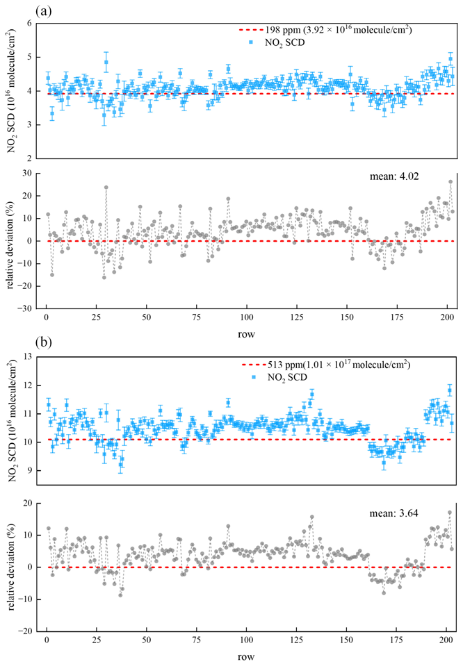
| Scattered sunlight | 198 | 4.08 × 10¹⁶ | 2.69 × 10¹⁵ | 1.40 × 10¹⁵ | 4.67 × 10¹⁴ |
| 513 | 1.05 × 10¹⁷ | 4.47 × 10¹⁵ | 1.59 × 10¹⁵ | 4.96 × 10¹⁴ | |
| Integrating sphere light | 198 | 3.83 × 10¹⁶ | 2.27 × 10¹⁵ | 4.28 × 10¹⁴ | 7.86 × 10¹³ |
| Reference Spectral | NO2 Gas (ppm) | Averaged NO2 SCD (Molecule/cm2) | Standard Deviation of NO2 SCD | Averaged NO2 Fitting Error (Molecule/cm2) | Standard Deviation of NO2 Fitting Error |
|---|---|---|---|---|---|
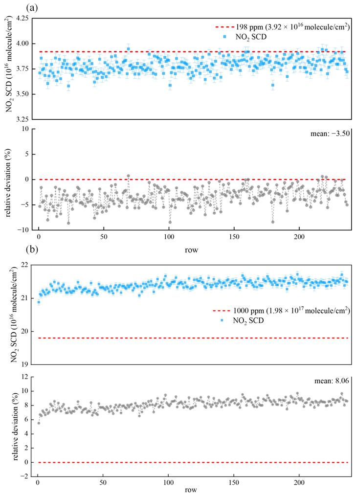
| tungsten halogen lamp | 198 | 3.64 × 10¹⁶ | 2.48 × 10¹⁵ | 1.48 × 10¹⁵ | 4.67 × 10¹⁴ |
| 1000 | 2.06 × 10¹⁷ | 4.27 × 10¹⁵ | 1.65 × 10¹⁵ | 4.96 × 10¹⁴ | |
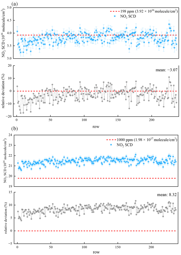
| Integrating sphere light | 198 | 3.69 × 10¹⁶ | 8.32 × 10¹⁴ | 4.80 × 10¹⁴ | 2.75 × 10¹³ |
| 1000 | 2.04 × 10¹⁷ | 1.70 × 10¹⁵ | 7.92 × 10¹⁴ | 1.10 × 10¹⁴ |
Publisher’s Note: MDPI stays neutral with regard to jurisdictional claims in published maps and institutional affiliations. |
© 2022 by the authors. Licensee MDPI, Basel, Switzerland. This article is an open access article distributed under the terms and conditions of the Creative Commons Attribution (CC BY) license (https://creativecommons.org/licenses/by/4.0/).
Share and Cite
Yang, T.; Si, F.; Zhou, H.; Zhao, M.; Lin, F.; Zhu, L. Preflight Evaluation of the Environmental Trace Gases Monitoring Instrument with Nadir and Limb Modes (EMI-NL) Based on Measurements of Standard NO2 Sample Gas. Remote Sens. 2022, 14, 5886. https://doi.org/10.3390/rs14225886
Yang T, Si F, Zhou H, Zhao M, Lin F, Zhu L. Preflight Evaluation of the Environmental Trace Gases Monitoring Instrument with Nadir and Limb Modes (EMI-NL) Based on Measurements of Standard NO2 Sample Gas. Remote Sensing. 2022; 14(22):5886. https://doi.org/10.3390/rs14225886
Chicago/Turabian StyleYang, Taiping, Fuqi Si, Haijin Zhou, Minjie Zhao, Fang Lin, and Lei Zhu. 2022. "Preflight Evaluation of the Environmental Trace Gases Monitoring Instrument with Nadir and Limb Modes (EMI-NL) Based on Measurements of Standard NO2 Sample Gas" Remote Sensing 14, no. 22: 5886. https://doi.org/10.3390/rs14225886
APA StyleYang, T., Si, F., Zhou, H., Zhao, M., Lin, F., & Zhu, L. (2022). Preflight Evaluation of the Environmental Trace Gases Monitoring Instrument with Nadir and Limb Modes (EMI-NL) Based on Measurements of Standard NO2 Sample Gas. Remote Sensing, 14(22), 5886. https://doi.org/10.3390/rs14225886